SISSA 13/2023/FISI

Abstract

We quantise from first principles field theories living on the background of a bubble wall in the planar limit with particular focus on the case of spontaneous breaking of gauge symmetry. Using these tools, we compute the average momentum transfer from transition radiation: the soft emission of radiation by an energetic particle passing across the wall, with a particular focus on the longitudinal polarisation of vectors. We find these to be comparable to transverse polarisations in symmetry-breaking transitions with mild super-cooling, and dominant in broken to broken transitions with thin wall. Our results have phenomenological applications for the expansion of bubbles during first order phase transitions. Our general framework allows for the calculation of any particle processes of interest in such translation breaking backgrounds.

1 Introduction

First order phase transitions (FOPTs) have long ago been proposed as having possibly occurred during the hot big-bang phase of the universe [1, 2, 3]. In the past, it was entertained that even within the known Standard Model (SM) of particle physics there might have been as many as two: chiral symmetry breaking/confinement in QCD at temperatures $T\sim 150\ \rm MeV$ and the spontaneous breaking of electroweak (EW) symmetry at $T\sim 160\ \rm GeV$. Both are now understood to be smooth crossovers [4, 5]. Infact, it is interesting to note that from the current laws of physics there is no conclusively established meta-stable vacuum for any temperature at zero chemical potential .

By contrast, FOPTs are ubiquitous in beyond the SM (BSM) theories. This is due firstly to a vast richness of important phenomenological consequences, among which baryogenesis[7, 8, 9, 10, 11, 12, 13, 14, 15, 16, 17, 18], the production of heavy dark matter[19, 20, 21, 22, 23, 24, 25], primordial black holes[26, 27, 28, 29, 30] and gravitational waves (GW)[3, 31, 32, 33, 34] to name a few. In particular, the EW phase transition is easily made first order in many BSM models[35, 36, 37, 38, 14, 39, 40, 41, 42, 43, 44, 45] and the consequent out-of-equilibrium dynamics (in conjunction with $B$ violation in the SM) still make for an attractive theory of baryogenesis. Secondly, our currently most compelling picture of physics at the highest energy scales seems to suggest landscapes of countless meta-stable vacua. From this perspective FOPTs may even be expected during the post-inflationary era [46]. Finally, and perhaps most importantly from a phenomenological perspective, the advent of gravitational wave detectors has re-energised interest in these violent phenomena with the prospect of upcoming experiments possibly detecting a stochastic gravitational wave background relic [3, 47, 48]. Thus even FOPTs occurring in potential hidden sectors decoupled from the SM and its thermal history become of interest [49, 50].

A FOPT proceeds through the nucleation and subsequent expansion of bubbles of new phase, pushed by the energy density difference $\Delta V$ between phases. If friction from the surrounding matter can be ignored, the bubble wall interpolating between the two phases will continue to expand with constant proper acceleration until they collide with each other, with most of the vacuum energy released thus going into kinetic energy of the walls. This scenario is known as runaway. If instead friction causes a pressure $\mathcal{P}$ which manages to equilibrate the driving force $\mathcal{P}\simeq\Delta V$, a constant subluminal terminal velocity is reached and energy is efficiently transferred to the medium. All phenomenological consequences listed above, for example the strength and spectral shape of the stochastic GW signal, depend crucially on the bubble velocity and which of the two regimes is realised. To this end, it becomes important to understand precisely the dynamics of an expanding domain wall in medium. The analysis of bubble-medium interactions is a complicated problem which is largely still under investigation [51, 52, 53, 54, 55, 56, 57, 58, 59, 60, 61, 62, 63, 64, 65, 66]. Friction is expected in general to be an involved function of bubble velocity $v_{w}$ and the surrounding degrees of freedom (d.o.f.). A distinction can be made however between low $v_{w}$, when a fluid description is most appropriate, and the ultra-relativistic regime, $\gamma_{w}\equiv 1/\sqrt{1-v_{w}^{2}}\gg L_{w}\Gamma_{\rm int.}$, where $L_{w}$ is the wall thickness in its rest frame and $\Gamma_{\rm int.}$ is the interaction rate between particles in medium [67]. We will focus on the latter regime in this work, where the wall can be said to be interacting with individual particles.

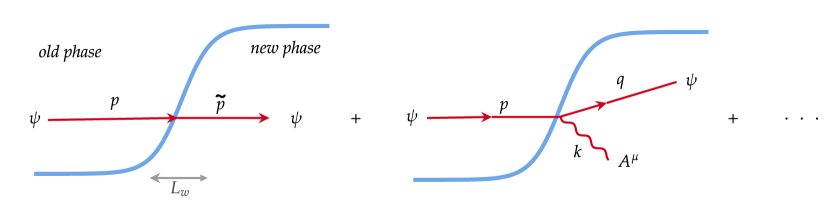
Figure 1: Diagrams corresponding to LO and NLO processes contributing to friction on a moving bubble wall. Emission of vectors with changing mass is generally the dominant $1\rightarrow 2$ process for friction and the subject of this work. Tilde distinguishes objects in the new phase.

A particle hitting the wall from the old phase can undergo many processes, which can be organised in terms of a perturbative expansion in couplings of the theory defined in the background of the wall profile, as sketched in fig. 1. The spontaneous breaking of translation symmetry means that momentum perpendicular to the wall is no longer conserved. The average momentum lost $\langle\Delta p\rangle$ times the flux of incoming particles is then the pressure opposing the bubble’s expansion. It is most convenient to work in the rest frame of the wall. At leading order (LO) incoming particles either cross the wall or reflect. It is easy to show that, when reflections can be neglected ,

$$\mathcal{P}^{\rm LO}_{\gamma_{w}\rightarrow\infty}\simeq(\gamma_{w}nv_{w})\langle\Delta p\rangle\simeq(\gamma_{w}nv_{w})\Delta m^{2}/2p^{0}\ ,$$ (1)

where $p^{0}\propto\gamma_{w}$ is the (boosted) incoming particle’s energy in the wall frame, $\Delta m\equiv\sqrt{\tilde{m}^{2}-m^{2}}$ the change in mass between phases, and $n$ the number density in the plasma frame. This LO pressure is independent of $\gamma_{w}$, scaling like $\propto T^{2}\tilde{v}^{2}$ in the case of a thermal bath, where $\tilde{v}$ is the vev in the broken phase [61, 62].

However, later the same authors analyzed the next-to-LO (NLO) $1\rightarrow 2$ processes in the same ultra-relativistic regime and found that, despite paying the price of the coupling, the emission of soft vector bosons that gain mass during the transition lead to a pressure/friction scaling like $\mathcal{P}^{\rm NLO}\propto\gamma_{w}$ [63], eventually dominating over the LO effect. This soft emission is known as transition radiation. While the original [63] focused on particles emitted forward into the wall (to the right in fig. 1), the authors of [69, 66] considered also reflected emission (to the left in fig. 1) and argued it was larger by a factor of four.

However, all studies after [63] only considered the emission of transverse vector polarisations, ignoring the effects of longitudinal ones. The analysis of these modes is complicated by the rearrangement of particle degrees of freedom across a gauge symmetry breaking transition [70], which has naturally been the case of greatest interest. Moreover, it is well known that amplitudes involving NGBs can give spurious divergences without proper care. Recently it was shown that LO effects from longitudinal modes can have a large impact on pressure [68]. It thus becomes of interest to properly account for their contribution at NLO. In addition, a weakness of the treatments used so far is the frequent reliance on WKB approximations, which are known to break down for the soft momenta dominating the emission phase space.

In this paper, we approach the calculation of transition radiation by quantising field theories in the Lorentz-violating background of a domain wall from first principles. A complete orthonormal basis is constructed out of ‘left’ and ‘right’ mover energy eigenstates , each wavemode having ‘reflected’ and ‘transmitted’ parts. We then carefully relate these to in and out asymptotic eigenstates of 4-momentum. In the case of vectors we show that the degrees of freedom across the wall are most conveniently described in terms of ‘wall polarisations’ $\tau$ and $\lambda$ rather than the conventional transverse and longitudinals, as already pointed out in [70]. The two sets coincide only for zero perpendicular momentum $\vec{k}_{\perp}=0$. The advantage is that $\tau_{1,2}$ and $\lambda$ are not mixed between each other in the presence of the domain wall . Moreover, in the case of gauge symmetry breaking, $\lambda$ smoothly interpolates between a Higgs d.o.f. on the symmetric side and a third massive vector d.o.f. on the broken side. We show how to perform calculations using this basis consistently and avoid divergences which seem to appear in a naive analysis.

Although we explain how to (numerically) compute $\langle{\Delta p}\rangle$ for a general wall profile, we dedicate most of the work to approximating it in a way that is independent of the particular shape, with the rough scale $L_{w}$ playing the only role, while commenting on the sensitivity thereon. For the IR of the emitted spectrum $k^{z}\lesssim L_{w}^{-1}$ the wall appears effectively as a step function. This limit is particularly interesting theoretically (as well as phenomenologically important, as mentioned already) since everything can be computed analytically and relatively simply. For wavelengths longer than the wall width $k^{z}>L_{w}^{-1}$, the WKB approximation becomes applicable. The integral over the phase space thus splits into two contributions and the averaged momentum exchange very schematically takes the form

$$\langle\Delta p\rangle\sim\int^{k^{z}<L_{w}^{-1}}{d^{3}k\>\Delta p}\;|\mathcal{M}^{\rm step}|^{2}\;+\;\int_{k^{z}>L_{w}^{-1}}{d^{3}k\>\Delta p}\;|\mathcal{M}^{\rm wkb}|^{2}\ .$$ (2)

where the $\mathcal{M}$ are matrix elements for emission calculated using the respective approximations. As the incoming flux scales like $\gamma_{w}$, we then have

$$\mathcal{P}\propto\gamma_{w}\langle\Delta p\rangle\ .$$ (3)

As a warm up, we study transition radiation in a theory with two scalars and observe some surprises. Though we find that the pressure from the emission of one scalar by the other always saturates at large velocities $\mathcal{P}^{\rm NLO,\rm scalars}_{\gamma_{w}\to\infty}\propto\gamma_{w}^{0}$, we find also that there can be a intermediate regime of linear growth $\mathcal{P}^{\rm NLO,\rm scalars}_{\rm intermediate}\propto\gamma_{w}$. Interestingly, for scalars we find that the WKB contribution (second term in eq. 2) dominates the momentum transfer in the asymptotic $\gamma_{w}$ limit.

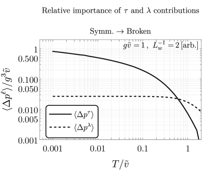
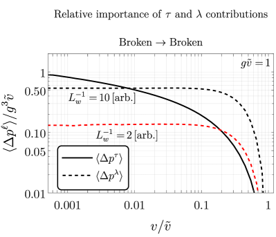
Figure 2: Comparison between the averaged exchanged momentum from transition radiation due to the emission of $\tau$ and $\lambda$ vector polarisations, in the limit of large incoming particle energy $p_{0}\to\infty$. Left: Symmetric $\to$ Broken transition in occuring at finite temperature $T$. Shown as a function of temperature over vev $\tilde{v}$. $T$ enters via thermal masses (for details see section 4.2). Results to not change significantly in the limit $L_{w}\rightarrow 0$. Right: Broken $\to$ Broken transition. While the $\tau$ contribution does not change, $\lambda$ emission can easily become dominant. We highlight the sensitivity on the wall thickness. [arb.] means arbitrary units.

In the case of spontaneous breaking of gauge symmetry we find that the total friction from vector emissions scales as $\propto\gamma_{w}\log\frac{gT}{\tilde{s}v}$ for $T/\tilde{v}\ll 1$ in line with literature. We provide an updated fitted formula in eqs. 146 and 4.3. The logarithmic enhancement appears only for the $\tau$ polarisations, and is dominated by the step function contribution (the first term in the eq. (2)), however we also find that effects of the $\lambda$ polarisations can lead to significant corrections for mild supercooling ($\frac{\tilde{v}}{T}\sim{\rm few}$). We compare the relative importance in fig. 2 (Left). The curves are only very weakly dependent on $L_{w}$.

As a side application, we also compute the transition radiation when the bubble wall connects two vacua with broken gauge symmetry but different vevs $v$ and $\tilde{v}$. In this case, the contribution to friction from the longitudinal vector emission scales as $\mathcal{P}^{\rm NLO,\rm vectors}_{\gamma_{w}\to\infty}\propto\gamma_{w}L_{w}^{-1}$ (see fig. 2, Right) and can dominate over the transverse for thin wall.

Aside from the asymptotic $p^{0}\rightarrow\infty$ limit, we are also able to explore regimes with intermediate - though large - $\gamma_{w}$. For symmetric $\to$ broken transition we find that the saturating value is reached at energies strongly dependent on the mass of the emitter particle, as shown in fig. 3 (Left). In the case of the broken $\to$ broken transition we find that there is an intermediate regime where the pressure scales as $\mathcal{P}^{\rm NLO,\rm vectors}_{\rm intermediate}\propto\gamma_{w}^{2}$ (right panel of fig. 3).

The paper is organised as follows: in the section 2 we work through a toy model with only scalars, introducing various elements of the calculation. In section 3 we quantise an Abelian Higgs model in the presence of a symmetry breaking domain wall, and present the results for transition radiation of vectors in section 4. We summarise in section 5.

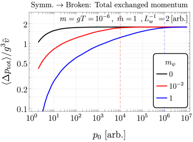
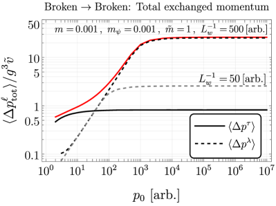
Figure 3: Total averaged momentum exchange as a function of incoming particle energy $p^{0}$. Left: Symmetric $\to$ Broken for different values of the mass of the emitter particle $\psi$. The asymptotic regime is reached around $p^{0}\sim m_{\psi}\tilde{m}/m$ (dashed lines), with intermediate $\log(p^{0}/m_{\psi})$ growth. Right: Broken $\to$ Broken with thin walls. Here the saturation value is reached around $p_{0}\sim L_{w}^{-1}{\rm Max}[1,m_{\psi}/m]$. Again we highlight the sensitivity to wall width. For small enough $L_{w}$ we find an inter-relativistic regime with averaged exchange momentum growing linearly, which translates to pressure scaling like $\gamma_{w}^{2}$.

Summary of notation:

In the rest of this paper, we will adopt the following conventions:

1. We treat the bubble wall in the planar limit where it is a domain wall centred around $z=0$.
   We use a hybrid notation for four-vector Lorentz indices:
   $\mu=(n,z)\equiv(0,1,2,z)$. Coordinates are $x^{\mu}=(x^{n},z)\equiv(t,\vec{x}_{\perp},z)$.

2. Similarly for mometa $k^{\mu}=(k^{n},k^{z})\equiv(k_{0},\vec{k}_{\perp},k^{z})\equiv(k_{0},\vec{k})$.
   Also $E^{2}=k^{n}k_{n}=k_{0}^{2}-k_{\perp}^{2}$, where $k_{\perp}=|\vec{k}_{\perp}|$.

3. We write the variation of mass across the wall $\Delta m\equiv\sqrt{\tilde{m}^{2}-m^{2}}$.

4. $L_{w}$ is the thickness of the wall.

5. $\gamma_{w}$ ($v_{w}$) is the boost factor (the velocity) of the wall.

6. The momenta $p,q,k$ will always be used as in fig. 1 and we define: [0pt]

   $$\begin{split}\Delta p\equiv p-q-k\ ,\quad\Delta p_{r}\equiv p-q+k\ ,\\ \Delta\tilde{p}\equiv p-q-\tilde{k}\ ,\quad\Delta\tilde{p}_{r}\equiv p-q+\tilde{k}\ .\end{split}$$ (4)

2 Simple example: scalars

In this section, as a warm up for the more physically relevant case of the emission of gauge bosons, we go through the quantised theory of scalars fields in the presence of the domain wall and derive results for transition radiation for the case of one scalar emitting another. This toy example is sufficient to highlight many features of the calculation.

Consider two different scalar fields $\phi,\psi$, the first of which feels the wall and has different mass depending on the phase, while the second for simplicity does not. The Lagrangian we consider is the following

$$\mathcal{L}={1\over 2}(\partial\phi)^{2}+{1\over 2}(\partial\psi)^{2}-{1\over 2}m^{2}_{\phi}(z)\phi^{2}-{1\over 2}m_{\psi}^{2}\psi^{2}-y(z)\frac{1}{2}\psi^{2}\phi,$$ (5)

where $m(z)$ interpolates between $m^{2}(z)|_{z\to-\infty}=m^{2}=const$ and $m^{2}(z)|_{z\to+\infty}=\tilde{m}^{2}=const$. Similarly $y(z)$ goes from $y$ to $\tilde{y}$. The profiles change on the scale of the wall width $L_{w}$ around $z=0$. The interactions in eq. (5) are not the most general, but are designed to mimic the vector case when $y=const$. The process that we will be studying is $\psi\to\psi\phi$, which would be forbidden by kinematics if it was not for the breaking of $z-$momentum.

Section summary:

In section 2.1 and 2.2, we quantise the free theory, focusing on the $\phi$ field , by defining a complete basis of solutions that solve its equations of motion. In section 2.3, we define a new basis which correspond to out-going eigenstates of momentum. Later, in section 2.4, we calculate the amplitude for the $\psi\to\psi\phi$ transition in the step wall approximation, valid when $k^{z}L_{w}\lesssim 1$. In section 2.5, we present the proper domain for the phase space integration over the final state. In section 2.6, we complete the emission spectrum discussing the calculation of the amplitude in the (opposite) WKB regime $k^{z}L_{w}\gtrsim 1$. In section 2.7, we summarise and present master formulae for the calculation of the averaged momentum transfer $\langle{\Delta p}\rangle$. We conclude discussing results for $\langle{\Delta p}\rangle$ and pressure $\mathcal{P}^{\rm NLO}$ in sections 2.8 and 2.9 respectively.

2.1 Complete basis

The quantisation of modes in the presence of a background profile arises in many corners of physics. A very similar task appears for example in the quantisation of field theory in black hole spacetimes. We found the treatment in [71] particularly useful. In the simple example of eq. (5) above, the discussion is relevant for $\phi$, which satisfies

$$(\partial^{2}+m_{\phi}^{2}(z))\phi=0\,,$$ (6)

with a $z-$dependent mass term. To perform second quantisation we need to first find a convenient basis of solutions of this equation. Far away from the wall the solution must become a plane wave. One in general can choose a complete basis of ‘right’ and ‘left’ moving solutions, which are defined as follows

$$\phi_{R,k}=e^{-ik_{n}x^{n}}\chi_{R,k}(z)\equiv e^{-ik_{n}x^{n}}\begin{cases}e^{ik^{z}z}+r_{R,k}e^{-ik^{z}z}\ ,&z\to-\infty\\ t_{R,k}e^{i\tilde{k}^{z}z}\ ,&z\to\infty\end{cases}\qquad\text{(Right)}$$ (7)

with $k^{0}>m$ and

$$\phi_{L,k}=e^{-ik_{n}x^{n}}\chi_{L,k}(z)\equiv e^{-ik_{n}x^{n}}\sqrt{k^{z}\over\tilde{k}^{z}}\begin{cases}t_{L,k}e^{-ik^{z}z}\ ,&z\to-\infty\\ r_{L,k}e^{i\tilde{k}^{z}z}+e^{-i\tilde{k}^{z}z}\ ,&z\to+\infty\end{cases}\qquad\text{(Left)}$$ (8)

with $k^{0}>\tilde{m}$ and we take $k^{z},\tilde{k}^{z}$ to be strictly positive . The factor $\sqrt{k^{z}/\tilde{k}^{z}}$ is included in eq. 8 to ensure appropriate normalisation (see below, eq. 14). In the limit of no domain wall the $r_{L},r_{R}$ ($t_{L},t_{R}$) coefficients are zero (one) and $\phi_{L},\phi_{R}$ correspond simply to the plane waves with $\mp k^{z}$ momenta. The momentum along $z$ is not conserved across the wall but asymptotically far from it becomes constant and fixed by the relations

$$k^{z}\equiv\sqrt{k_{0}^{2}-k_{\perp}^{2}-m^{2}},~{}~{}\tilde{k}^{z}\equiv\sqrt{k_{0}^{2}-k_{\perp}^{2}-\tilde{m}^{2}}.$$ (9)

In general, we need to solve the equations of motion to find the expression of the coefficients $r_{L,R},t_{L,R}$. Consequently, they will depend on the explicit form of the mass variation $m^{2}_{\phi}(z)$. However, here it will be sufficient to consider the step wall ansatz for the mass $m_{\phi}^{2}(z)$

$$m_{\phi}^{2}(z)=m^{2}+\Delta m^{2}\Theta(z)\,,\qquad\Delta m^{2}\equiv\tilde{m}^{2}-m^{2}\,.$$ (10)

using the Heaviside Theta function. The form of the coefficients for the scalar case under consideration can be obtained via matching at the origin $z=0$, where the step wall lies, and take the form

$$r_{R,k}=\frac{k^{z}-\tilde{k}^{z}}{k^{z}+\tilde{k}^{z}}\ ,\quad t_{R,k}=\frac{2k^{z}}{k^{z}+\tilde{k}^{z}}\ .$$ (11)

These expressions are specific to the step-wall assumption, however the general treatment that we present here will hold for general $r_{k},t_{k}$ coefficients and could be easily adapted to a smooth wall case. Modes with $m<k_{0}<\tilde{m}$ decay exponentially on the right of the wall and are automatically included as right-movers. For these, $\tilde{k}$ is purely imaginary with magnitude

$$|\tilde{k}^{z}|^{2}=\Delta m^{2}-k_{z}^{2}\qquad\text{for}\qquad 0<k^{z}<\Delta m\ .$$ (12)

In a similar fashion, for the left moving solution we find

$$r_{L,k}=-{r}_{R,k}=\frac{\tilde{k}^{z}-k^{z}}{k^{z}+\tilde{k}^{z}}\ ,\quad t_{L,k}=\frac{\tilde{k}^{z}}{k^{z}}t_{R,k}=\frac{2\tilde{k}^{z}}{k^{z}+\tilde{k}^{z}}\ .$$ (13)

and we explicitly note the condition $k_{0}>\tilde{m}$, to avoid the inclusion of solutions growing exponentially at infinity. The left and right moving modes are orthonormal in the sense that

$$\int_{-\infty}^{\infty}dz\;\chi_{I,k}\;\chi_{J,q}^{*}=2\pi\delta_{IJ}\delta(k^{z}-q^{z})\ ,\qquad I,J\in\{R,L\}\ .$$ (14)

Computing the integral in eq. 14 - among many other things - in the step function case requires the identity

$$\int_{-\infty}^{0}e^{i\beta z}dz={\rm PV}\left(\frac{1}{i\beta}\right)+\pi\delta(\beta)\ ,$$ (15)

and its complex conjugate (which gives the integral from $0$ to $\infty$). In eq. (14) the principle value (PV) pieces vanish as soon as we specify the relation between $\tilde{k}^{z}$ and $k^{z}$, i.e. $\tilde{k}_{z}^{2}=k_{z}^{2}+m^{2}-\tilde{m}^{2}$. Notice these relations only hold because we can discard terms proportional to $\delta(k^{z}+q^{z})$ due to the strictly positive definition of $k^{z},q^{z}$ in our definition. If explicitly computing things like the Hamiltonian and operator algebra (see next subsection) it is also useful to know the other inner products:

$$\int_{-\infty}^{\infty}dz\;\chi_{R,k}\;\chi_{R,q}=-\int_{-\infty}^{\infty}dz\;\chi_{L,k}\;\chi_{L,q}=2\pi{k^{z}-\tilde{k}^{z}\over k^{z}+\tilde{k}^{z}}\delta(k^{z}-q^{z}),$$

$$\int_{-\infty}^{\infty}dz\;\chi_{R,k}\;\chi_{L,q}=4\pi{\sqrt{k^{z}\tilde{k}^{z}}\over k^{z}+\tilde{k}^{z}}\delta(k^{z}-q^{z}).$$ (16)

Finally, we would like to comment that in general a discrete number of bound states may appear in the spectrum, in addition to the scattering states studied above, if the function $m^{2}_{\phi}(z)$ is non-monotonic and has minima in the vicinity of the domain wall. These are of the form $\phi_{\rm b}\propto e^{-ik^{n}x_{n}}\chi_{\rm b}(z)$, with $\chi_{\rm b}$ exponentially decaying for $|z|\rightarrow\infty$ and should be included in the upcoming expansion section 2.2.

2.2 Quantisation

Now that we have a complete orthonormal basis of eigenstates in the presence of the wall, we can proceed to quantise the theory. The field $\phi$ can be expanded in the form

$$\phi(x,t)=\sum_{I=R,L}\int\frac{d^{3}k}{(2\pi)^{3}\sqrt{2k_{0}}}\left(a_{I,k}\phi_{I,k}+a^{\dagger}_{I,k}\phi^{*}_{I,k}\right),$$

$${\rm where}\quad\phi_{L,k}\equiv 0\quad\text{for}\quad E<\tilde{m}\ ,$$ (17)

where $d^{3}k\equiv dk^{z}d^{2}k_{\perp}$, we defined $E\equiv\sqrt{k_{0}^{2}-k_{\perp}^{2}}$ and $k^{z}$ is varied between $[0,\infty)$. We choose to label states by their quantum numbers outside the wall. Note we have trivially extended the definition of the left moving modes to the region $E<\tilde{m}$ for convenience.

Using eqs. 14 and 16, one can show that

$$a_{I,p}=\int{dz\over\sqrt{2p_{0}}}e^{ip_{0}t}\chi^{*}_{I,p}(i\pi+p_{0}\phi)\ ,$$ (18)

where $\pi\equiv\partial_{t}\phi$. Promoting Poisson brackets of $\phi$ and its conjugate momentum $\pi$ to canonical commutation relations gives the familiar commutation algebra

$$\begin{split}[a_{I,k},a_{J,q}^{\dagger}]&=(2\pi)^{3}\delta(\vec{k}-\vec{q})\delta_{IJ}\ ,\\ [a_{I,k},a_{J,q}]&=[a_{I,k}^{\dagger},a_{J,q}^{\dagger}]=0\ ,\qquad I,J\in\{R,L\}\ .\end{split}$$ (19)

We can define two types of states

$$\left|k_{R}\right\rangle \equiv\sqrt{2k_{0}}\;a_{R,k}^{\dagger}\left|0\right\rangle\ ,$$ (20)

$$\left|k_{L}\right\rangle \equiv\sqrt{2k_{0}}\;a_{L,k}^{\dagger}\left|0\right\rangle\ ,$$ (21)

which should be thought of as independent external states in any process. The space of physical states is thus the Fock space defined by arbitrary powers of $a_{R,k}^{\dagger}$ and $a_{L,k}^{\dagger}$ acting on the vacuum.

2.3 Out-going eigenstates of momenta

In the previous subsections we chose to quantise the orthonormal basis $\{\phi_{R,k}\>,\phi_{L,k}\}$ and defined associated one-particle states $\left|k_{R}\right\rangle$ and $\left|k_{L}\right\rangle$. As we explain in more detail in appendix A by the use of wave-packets, these should be thought of as describing incoming particles with definite $z-$momenta $k^{z}$ and $-\tilde{k}^{z}$ respectively at $t\to-\infty$, but at $t\to+\infty$ they correspond to a superposition between a transmitted and reflected particle. As a consequence, the functions $\phi_{R,L}$ are eigenstates of momenta only at $t\to-\infty$. They are well-suited for processes with asymptotic in-state $\phi$ particles.

On the other hand, in this work we will be interested in the momentum transfer to the wall, so it is more convenient to have a $\phi$ particle emitted as an asymptotic out-state with well-defined momentum at $t\to\infty$. A complete orthonormal basis of such late-time eigenstates of momentum is given by

$$\phi^{\rm out}_{L,k} \equiv e^{-ik_{n}x^{n}}\zeta_{L,k}(z)=e^{-ik_{n}x^{n}}\chi_{R,k}^{*}(z)=e^{-ik_{n}x^{n}}\left(r_{R,k}^{*}\;\chi_{R,k}+t_{R,k}^{*}\sqrt{\frac{\tilde{k}^{z}}{k^{z}}}\;\chi_{L,k}\right)\ ,$$ (22)

$$\phi^{\rm out}_{R,k} \equiv e^{-ik_{n}x^{n}}\zeta_{R,k}(z)=e^{-ik_{n}x^{n}}\chi_{L,k}^{*}(z)=e^{-ik_{n}x^{n}}\left(r_{L,k}^{*}\;\chi_{L,k}+t_{L,k}^{*}\sqrt{\frac{k^{z}}{\tilde{k}^{z}}}\;\chi_{R,k}\right)\ ,$$ (23)

where in the last equalities we related them to the basis of section 2.1. We emphasise again that in our notation $k^{z},\tilde{k}^{z}>0$ always. $\phi^{\rm out}_{L,k}$ and $\phi^{\rm out}_{R,k}$ should be thought of as describing an outgoing final state particle with $-k^{z}$ and $+\tilde{k}^{z}$ momentum respectively. Remember that the function $\chi_{L,k}$ vanishes for $k^{z}<\Delta m$ and the corresponding $\Theta$ functions are implicit. At $t\to-\infty$ they are both superpositions of incoming particles from $z=\pm\infty$ and do not have well defined momentum. In practice we need to calculate the amplitudes with $\zeta_{L,R}=\chi^{*}_{R,L}$ wave functions. At the level of states we have

$$|k^{\rm out}_{L}\rangle =r_{R,k}^{*}|k_{R}\rangle+t_{R,k}^{*}\sqrt{\tilde{k}^{z}/k^{z}}\;|k_{L}\rangle\;\Theta(k^{z}-\Delta m)\ ,$$ (24)

$$|k^{\rm out}_{R}\rangle =t_{L,k}^{*}\sqrt{k^{z}/\tilde{k}^{z}}\;|k_{R}\rangle+r_{L,k}^{*}|k_{L}\rangle\ ,$$ (25)

where we explicitly remind ourselves that when $0<k^{z}<\Delta m$ the left mover state does not exist. The different asymptotic states are illustrated in the fig. 4.

We emphasise that which basis is used to quantise the theory is completely arbitrary and should be chosen according to the problem at hand. In our present paper we will consider only outgoing $\phi$ particles so that the basis $\{\phi^{\rm out}_{R,k},\phi^{\rm out}_{L,k}\}$ is actually more convenient. Either way the results will be the same. From now on we drop the label ‘out‘ and we will refer to $R$ ($L$) emission meaning using the mode functions $\{{\zeta_{R}},{\zeta_{L}}\}$, if not stated otherwise.

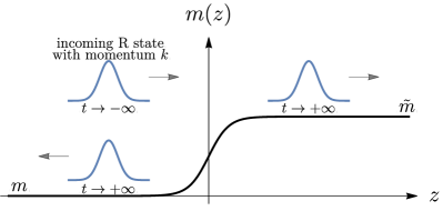
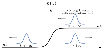
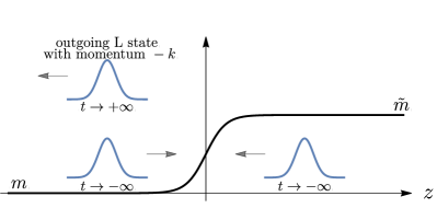
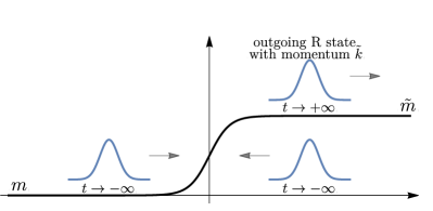
Figure 4: Summary of asymptotic external states with definite $4-$momentum, to be used in calculating any process in the background of a domain wall (or any localised $z-$dependent potential). The upper panels represent in-state particles incoming from $z=-\infty$ and $z=\infty$. In the plane wave limit they correspond to states $\left|k_{R}\right\rangle$ and $\left|k_{L}\right\rangle$ with wavefunctions eqs. 7 and 8 respectively. The lower panels represent out-state particles travelling out towards $z=-\infty$ and $z=\infty$. They correspond to states eqs. 24 and 25 with wavefunctions eqs. 22 and 23 respectively.

2.4 Amplitudes

We now finally turn to computing the amplitude for the process $\psi\to\psi\phi$ in the background of a domain wall. We have not discussed the quantisation of $\psi$ since it does not feel the wall directly and there are no complications with respect to the standard theory. In the previous sections we argued that there are two processes we have to consider separately: the emission of a left and right moving $\phi$ particle, with respective wavefunctions $\zeta_{L}(\zeta_{R})$. Having quantised the free theory, the treatment of perturbative interactions proceeds as standard, by defining an $S$-matrix in terms of the interaction Hamiltonian $\mathcal{S}={\rm T\;exp}\left(-i\int d^{4}x\mathcal{H}_{\rm Int}\right)$ where T here denotes time ordering, we have the amplitude of interest

$$\langle k_{I}^{\rm out}\;q|\>\mathcal{S}\>|p\rangle \equiv(2\pi)^{3}\delta^{(3)}(p^{n}-k^{n}-q^{n})i\mathcal{M}_{I}\overset{\rm tree}{=}-i\int d^{4}x\langle k_{I}^{\rm out}\;q|\ \mathcal{H}_{\rm Int}\ |p\rangle$$ (26)

$$\text{with}\quad I =L,R\ ,$$

where $p$ and $q$ stand for the initial and final one particle states for the $\psi$ field and their respective $4-$momenta, and the last equality is up to leading order in perturbation theory (tree level). Notice we have defined the matrix element $\mathcal{M}$ as closely as possible to standard theory. Of course we cannot extract a $z-$momentum conserving delta function but rather $\mathcal{M}$ still contains the integral over $z$.

For the theory of scalars of eq. 5, we have $\mathcal{H}_{\rm Int}=-iy\psi^{2}(x)\phi(x)$ and we can now proceed to explicitly computing amplitudes. In the case of a ${\zeta_{L}}$ mode emission (where the emitted scalar has $-k^{z}$ momentum), the amplitude takes the form

$$\mathcal{M}_{L} =\int_{-\infty}^{\infty}dz\;y(z)e^{i(p^{z}-q^{z})z}\left[\zeta_{L,k}=\chi^{*}_{R,k}(z)\right]^{*}$$

$$=\left[\frac{-iy}{p^{z}-q^{z}+k^{z}}+r_{R,k}\frac{-iy}{p^{z}-q^{z}-k^{z}}-t_{R,k}\frac{-i\tilde{y}}{p^{z}-q^{z}+\tilde{k}^{z}}\right]\ .$$ (27)

Instead, in the case of ${\zeta_{R}}$ mode emission (where the emitted scalar has $+\tilde{k}^{z}$ momentum):

$$\mathcal{M}_{R} =\int_{-\infty}^{\infty}dz\;y(z)e^{i(p^{z}-q^{z})z}\left[\zeta_{R,k}=\chi^{*}_{L,k}(z)\right]^{*}$$

$$=\sqrt{\frac{k^{z}}{\tilde{k}^{z}}}\left[t_{L,k}\frac{-iy}{p^{z}-q^{z}-k^{z}}-\frac{-i\tilde{y}}{p^{z}-q^{z}-\tilde{k}^{z}}-r_{L,k}\frac{-i\tilde{y}}{p^{z}-q^{z}+\tilde{k}^{z}}\right]\ ,$$ (28)

where the square root factor comes from the normalisation condition in eq. 8. We emphasise that to compute the total friction from $\psi\rightarrow\psi\phi$ we must sum the contributions from both processes. Then we can compute the amplitude squared for the emission of a right/left mover, under the assumption that $y=const.$, we obtain

$$|\mathcal{M}_{R}|^{2} =y^{2}{4k^{z}\tilde{k}^{z}(k^{z}-\tilde{k}^{z})^{2}\over(\tilde{k}_{z}^{2}-(p^{z}-q^{z})^{2})^{2}(k^{z}-p^{z}+q^{z})^{2}}\ ,$$ (29)

$$|\mathcal{M}_{L}|^{2} =y^{2}{4k_{z}^{2}\over(k_{z}^{2}-(p^{z}-q^{z})^{2})^{2}}\begin{cases}{(k^{z}-\tilde{k}^{z})^{2}\over(\tilde{k}^{z}+p^{z}-q^{z})^{2}}\ ,&k^{z}>\Delta m\ ,\\ {\Delta m^{2}\over\Delta m^{2}-k_{z}^{2}+(p^{z}-q^{z})^{2}}\ ,&k^{z}<\Delta m\ ,\end{cases}$$ (30)

where for $L$ emission we distinguished between the two branches corresponding to $\tilde{k}^{z}$ purely real and imaginary, and used eq. 12 to simplify in the latter case. The physical interpretation of left and right movers is straightforward. We can see the right movers as a particle emitted and then transmitted inside the bubble wall, while the left movers is a particle first emitted and then reflected by the wall outside.

2.5 Phase Space integration

We can now compute the averaged exchanged momentum, $\langle\Delta p\rangle$, times the amplitude for a $\psi$ particle to emit a $\phi$ and integrate over the phase space of the final particles. $\langle\Delta p\rangle(p)$, which is a priori a function of the four-momentum $p$ of the incoming $\psi$, thus represents an average of the momentum exchanged over one interaction. Then, from $\langle\Delta p\rangle$ we will be able to compute the total friction thereof, by adding separately contributions from left and right movers with their respective slightly different allowed phase spaces and integrating over the incoming flux.

Having in mind $1\to 2$ processes and the fact that we have been labelling the mode functions as a function of $k^{z}\ (>0)$ we will parameterise the kinematic of the process and the following phase space integration in term of the variables $(k^{z},k_{\perp})$. Then

$$p^{\mu}=(p_{0},0,0,\sqrt{p_{0}^{2}-m_{\psi}^{2}}),\qquad q^{\mu}=(q_{0},0,k_{\perp},q^{z}),$$ (31)

$$k^{\mu}=(k_{0},0,-k_{\perp},k^{z}),\qquad \tilde{k}^{\mu}=(k_{0},0,-k_{\perp},\tilde{k}^{z}),$$

where $\tilde{k}^{z}$ is defined in eq. (9), $q^{z}=\sqrt{q_{0}^{2}-k_{\perp}^{2}-m_{\psi}^{2}}$, while from the energy conservation we can write $q_{0}=p_{0}-k_{0}$. Note we have used the cylindrical symmetry of the set up to make the first spatial component of the momentum zero. The averaged exchange of momentum $\langle\Delta p\rangle$ is given by the sum of the left and the right moving contributions, being independent external states in any process,

$$\langle\Delta p\rangle =\langle\Delta p_{R}\rangle+\langle\Delta p_{L}\rangle$$

$$\equiv\int d\mathbb{P}_{\psi\rightarrow\psi\phi_{R}}\underbrace{(p^{z}-q^{z}-\tilde{k}^{z})}_{\Delta p^{z}_{R}}+\int d\mathbb{P}_{\psi\rightarrow\psi\phi_{L}}\underbrace{(p^{z}-q^{z}+k^{z})}_{\Delta p^{z}_{L}}\ .$$ (32)

where $d\mathbb{P}_{\psi\rightarrow\psi\phi_{I}}$ is the differential probability. We emphasise that the two phase spaces, respectively in the first and the second terms on the RHS of section 2.5, will be different in their lower limits on the $k^{z}$ integrals. The second term, the left-mover, contains also the contribution from modes which are exponentially decaying inside the wall. For the terms on the RHS of section 2.5, the right mover, we obtain

$$\int d\mathbb{P}_{\psi\rightarrow\psi\phi_{I}}\Delta p^{z}_{I}=\int_{k^{z,I}_{\rm min}}^{k^{z}_{\rm max}}\dfrac{dk_{z}}{2\pi}{1\over 2k_{0}}\int_{0}^{k_{\perp,\rm max}^{2}}\ \dfrac{dk_{\perp}^{2}}{4\pi}\cdot\dfrac{1}{2p^{z}}\left[\dfrac{1}{2|q^{z}|}|\mathcal{M}_{I}|^{2}\Delta p^{z}_{I}\right]_{q^{z}=\pm q_{k}^{z}},$$ (33)

where $I=R,L$ and $\left[...\right]_{q^{z}=\pm q_{k}^{z}}$ is intended to be the sum over $q^{z}=\pm q_{k}^{z}$. The contribution with $q^{z}=-q_{k}^{z}$ corresponds to reflection of the incoming particle $\psi$ (see for details defined in Appendix A.2), and we believe it was missing in the previous literature. Of course in the ultra-relativistic regime this should be highly suppressed. However the contribution could be relevant for amplitudes which are sensitive to the width of the wall even in the regime $m\ll p_{0}\ll L_{w}^{-1}$. Notice that although the amplitude is suppressed, the sign change in $\Delta p^{z}_{R}$ means that for a given $q_{0}$ and a given interaction, the $q^{z}<0$ process contributes more to momentum exchange, as the exchange of momentum is larger.

The limits of integration of eq. 33 are different between $R$ and $L$ emission and are found ensuring the energy conservation alongside the reality of the $q^{z}$ momentum, obtaining for the $(R)$ modes

$$(R): k^{z,R}_{\rm min}\equiv\Delta m\leq k^{z}\leq k^{z}_{\rm max}\equiv\sqrt{(p_{0}-m_{\psi})^{2}-m^{2}},$$ (34)

$$0\leq k_{\perp}^{2}\leq k_{\perp,\rm max}^{2}\equiv{1\over 4p_{0}^{2}}(p_{0}^{2}+k_{z}^{2}+m^{2}-m_{\psi}^{2})^{2}-k_{z}^{2}-m^{2}.$$

For what concern the limits of integration for the $(L)$ modes, the only difference is in the lower limit of $k^{z}$ integration, where we need also to consider exponentially decaying modes inside the wall, that is

$$(L):\quad k^{z,L}_{\rm min}\equiv 0 \leq k^{z} \leq k^{z}_{\rm max}\ .$$ (35)

Following this discussion in general there will be four contributions:

$$\langle\Delta p^{q^{z}<0}_{L}\rangle,\langle\Delta p^{q^{z}>0}_{L}\rangle,\langle\Delta p^{q^{z}<0}_{R}\rangle,\langle\Delta p^{q^{z}>0}_{R}\rangle.$$

We explicitly checked that in all the regimes we are interested the contributions with $q^{z}<0$ are largely subdominant and we will ignore them completely in the rest of this paper.

2.6 Emission in the WKB regime

So far we have been treating the bubble wall as a step function. This is a good approximation if the $z$ momentum of the emitted particle is less than the inverse width of the wall, i.e. $k^{z}<L_{w}^{-1}$, where $L_{w}$ is the typical width of the wall i.e. the region where the mass varies significantly. How can we proceed if the particles momentum becomes comparable or larger than the width of the wall?

First of all, if we know the shape of the potential exactly we can solve for the left and right mover solutions as we have done above for the step-wall, and proceed with these functions in precisely the same way as before. In principle this can be done numerically, if the potential is known. However even in the case when we do not know the exact shape of the potential we can still obtain reliable results. Let us consider a particle hitting the wall with the momentum $k^{z}\gg L_{w}^{-1}$ much larger than the parametric wall width $L_{w}$. At those large energies, the step wall approximation is not valid anymore, reflection will be suppressed and WKB approximation becomes applicable [63, 65, 66]. We can use approximate solutions to the $\chi_{R,L}(\zeta_{R,L})$ basis functions using WKB approximation, and then proceed in the same way as in the section 2.4. In practice this means that we need to separate the phase space into two regions and apply two different approaches:

$$\hbox{region (1)}~{}~{}~{}~{}~{}~{}~{}~{}k^{z}_{\phi}\ll L_{w}^{-1},~{}~{}~{}\hbox{step wall, \quad}$$

$$\hbox{region (2)}~{}~{}~{}~{}~{}~{}~{}~{}k^{z}_{\phi}\gg L_{w}^{-1}~{}~{}~{}~{}\hbox{WKB. \quad}$$ (36)

In the WKB regime there reflection is suppressed and the amplitude can be schematically written as follows

$${\cal M}_{\rm wkb} = \int_{-\infty}^{+\infty}dzV(z)\exp\left[i\int_{0}^{z}\Delta p(z^{\prime})dz^{\prime}\right]\prod_{i}\sqrt{\frac{p^{i}_{z}(0)}{p^{i}_{z}(z)}}\ ,$$

$$\Delta p(z^{\prime}) \equiv \sum_{i}p^{i}_{z}(z^{\prime})=\sum_{i}\sqrt{(p^{i}_{0})^{2}-(p^{i}_{\perp})^{2}-m_{i}^{2}(z^{\prime})}\ ,$$ (37)

Calculation of this integral requires the knowledge of the functions $m_{i}(z)$. However in the background of the domain wall this functions are changing only in the vicinity of the wall and outside quickly reach the asymptotic constant values. This means we can split the amplitude into two pieces

$$\mathcal{M}^{\rm wkb}= \underbrace{\int_{-\infty}^{0}dzV(-\infty)e^{i\Delta p_{z}(-\infty)z}+e^{i\int_{0}^{L_{w}}dz^{\prime}\Delta p(z^{\prime})}\int^{\infty}_{0}dzV(+\infty)e^{i\Delta p_{z}(+\infty)z}}_{\mathcal{M}_{\rm outside}}$$

$$+ \underbrace{\int^{L_{w}}_{0}dzV(z)e^{i\int_{0}^{z}dz^{\prime}\Delta p(z^{\prime})}}_{\mathcal{M}_{\rm inside}}\ ,$$ (38)

where the assumption is that domain wall is essentially present only between $z\in[0,L_{w}]$. In WKB regime all the momenta of the particles are much larger than inverse width of the wall $p^{z}L_{w}\gg 1$ so the overall modification of momenta $p(+\infty)-p(-\infty)\ll p(\infty)$ is much less than its absolute value (if the wall is not too thick $m(z)L\lesssim 1$), this is why we have approximated $\prod\sqrt{p/p(z)}\to 1$. Similarly $\Delta p(+\infty)-\Delta p(-\infty)\ll\Delta p(\infty)$, then from basic properties of Fourier transformations the amplitude

$${\cal M}\to 0,\hbox{ if }\Delta p_{z}^{\rm max}L_{w}\gg 1\ ,$$ (39)

with $\Delta p_{z}^{\rm max}={\rm Max}[\Delta p_{z}(\pm\infty)]$. The physics behind this relation is very simple: the wall of the width $L_{w}$ can lead to the momentum loss $\Delta p_{z}$ at most $L_{w}^{-1}$. This is expected since the processes with $\Delta p_{z}\gg L_{w}^{-1}$ happen at distances $\sim\Delta p_{z}^{-1}$ much shorter than the typical wall width, however at such small distances we recover Lorentz symmetry along the $z$ direction and transition radiation must be forbidden (we checked these statements for various wall ansatzes in appendix H). From these arguments we can see that independently of the wall ansatz the particle emission will be dominated by the region $\Delta p_{z}L_{w}\lesssim 1$. Then we can approximate the amplitude as follows

$$\mathcal{M}^{\rm wkb}= \int_{-\infty}^{0}dzV(-\infty)e^{i\Delta p_{z}(-\infty)z}+\int^{\infty}_{0}dzV(+\infty)e^{i\Delta p_{z}(+\infty)z}$$

$$+ \int^{L_{w}}_{0}dzV(z)e^{i\int d\tilde{z}\Delta p(\tilde{z})}\ .$$ (40)

Performing the $z$ integrals for the first two terms is trivial and we get

$$\mathcal{M}^{\rm wkb}\approx\frac{V(-\infty)}{i\Delta p_{z}(-\infty)}-\frac{V(+\infty)}{i\Delta p_{z}(+\infty)}+\int^{L_{w}}_{0}dzV(z)e^{i\int d\tilde{z}\Delta p(\tilde{z})}\ .$$ (41)

The last term scales very roughly as $V(z\in[0,L_{w}])L_{w}$ then assuming $V(z\in[0,L_{w}])\sim V(\infty)\sim V(-\infty)$ we can see it will be suppressed by the condition $\Delta pL_{w}\lesssim 1$. Thus we arrive at the Bodeker-Moore formula [63] for reduced matrix element

$$\mathcal{M}^{\rm wkb\;red.}=\frac{V(-\infty)}{i\Delta p_{z}(-\infty)}-\frac{V(+\infty)}{i\Delta p_{z}(+\infty)}\ .$$ (42)

Now we can take this formula and perform the phase space integration. However we would like to emphasise simple but important detail about the calculations. Since we have ignored the part inside the wall there is no guarantee that the matrix element will be suppressed in the region with $\Delta p_{z}L_{w}\gg 1$. In all of our calculations we always:

• impose $\Delta p_{z}L_{w}<1$ $-$ Fourier decomposition properties

• verify that ${\cal M}_{\rm inside}\ll{\cal M}_{\rm outside}$ $-$ applicability of BM approximation (we anticipate here that satisfying this inequality turns out to be non-trivial for the longitudinal vector bosons).

Finally, from this discussion it is clear that we should not worry about left emission in the WKB approximations since for left movers with $k^{z}>L_{w}^{-1}$ the total loss of momenta $\Delta p_{z}=p^{z}-q^{z}+k^{z}>L_{w}^{-1}$, thus these processes must be strongly suppressed and we can safely ignore them.

Scalars example

Let us apply this very generic discussion to the case of scalar radiation. Then the matrix element will be given by

$${\cal M}^{\rm wkb\;red.}=\frac{-iy}{p^{z}-q^{z}-k^{z}}-\frac{-iy}{p^{z}-q^{z}-\tilde{k}^{z}}\,\ ,$$ (43)

for the contribution outside of the wall. The contribution inside the wall (which we ignore) scales roughly as

$$\frac{{\cal M}^{\rm inside}_{\rm wkb}}{{\cal M}^{\rm wkb\;red.}}\sim\Delta p_{z}L_{w}\ ,$$ (44)

which is always less than one. We conclude that the neglected corrections coming from inside of the wall contributions are indeed negligible for scalars.

2.7 Procedure for the momentum transfer calculation: summary

In this section we summarise the previous discussion and results and give a concise prescription for the momentum transfer calculation. There are three types of contributions:

$$\langle{\Delta p_{L}^{\rm step}}\rangle\ ,~{}~{}\langle{\Delta p_{R}^{\rm step}}\rangle\ ,~{}~{}\langle{\Delta p^{\rm wkb}}\rangle\ ,$$ (45)

where the first two correspond to the $L,R$ emission in the step wall approximation and the last one to the $R$ emission in WKB regime. These momentum transfers are given by the following phase space integrals:

$$\langle{\Delta p_{L}^{\rm step}}\rangle= \int_{0}^{k^{z}_{\rm max}}\dfrac{dk_{z}}{2\pi}{1\over 2k_{0}}\int_{0}^{k_{\perp,\rm max}^{2}}\ \dfrac{dk_{\perp}^{2}}{4\pi}\cdot\dfrac{1}{2p^{z}}\left[\dfrac{1}{2|q^{z}|}|\mathcal{M}_{L}|^{2}(p^{z}-q^{z}+k^{z})\right]\Theta(L_{w}^{-1}-k^{z})\ ,$$

$$\langle{\Delta p_{R}^{\rm step}}\rangle= \int_{\Delta m}^{k^{z}_{\rm max}}\dfrac{dk_{z}}{2\pi}{1\over 2k_{0}}\int_{0}^{k_{\perp,\rm max}^{2}}\ \dfrac{dk_{\perp}^{2}}{4\pi}\cdot\dfrac{1}{2p^{z}}\left[\dfrac{1}{2|q^{z}|}|\mathcal{M}_{R}|^{2}(p^{z}-q^{z}-\tilde{k}^{z})\right]\Theta(L_{w}^{-1}-k^{z})\ ,$$

$$\langle{\Delta p^{\rm wkb}}\rangle= \int_{\Delta m}^{k^{z}_{\rm max}}\dfrac{dk_{z}}{2\pi}{1\over 2k_{0}}\int_{0}^{k_{\perp,\rm max}^{2}}\ \dfrac{dk_{\perp}^{2}}{4\pi}\cdot\dfrac{1}{2p^{z}}\left[\dfrac{1}{2|q^{z}|}|\mathcal{M}^{\rm wkb\;red.}|^{2}(p^{z}-q^{z}-\tilde{k}^{z})\right]$$

$$\times\Theta\left(k^{z}-L_{w}^{-1}\right)\Theta\left(L_{w}^{-1}-(p^{z}-q^{z}-\tilde{k}^{z})\right)\ ,$$ (46)

where the limits $k^{z}_{\rm max},k_{\perp,\rm max}^{2}$ were defined in eq. (34) but we repeat them here for the reader’s convenience,

$$k_{z}^{\rm max}\equiv\sqrt{(p_{0}-m_{\psi})^{2}-m^{2}}\ ,$$

$$k_{\perp,\rm max}^{2}\equiv{1\over 4p_{0}^{2}}(p_{0}^{2}+k_{z}^{2}+m^{2}-m_{\psi}^{2})^{2}-k_{z}^{2}-m^{2}\ .$$ (47)

and also recall that $\Delta m^{2}\equiv\tilde{m}^{2}-m^{2}$. $\mathcal{M}_{L},\mathcal{M}_{R}$ are the amplitudes for the process calculated using the step wall ansatz (see section 2.4) and $\mathcal{M}^{\rm wkb\;red.}$ is the amplitude in the WKB approximation, without the contribution inside the wall, calculated following the discussion in section 2.6. Note the presence of various Theta functions imposing cuts on phase space. For the $\langle{\Delta p_{{L,R}}^{\rm step}}\rangle$ cases these ensure that $k^{z}<L_{w}^{-1}$, i.e. step wall approximation is valid. For the WKB case the first step function $\Theta(k^{z}-L_{w}^{-1})$ comes from requirement of validity of WKB, i.e. large momentum compared to the wall width. The second step function $\Theta\left(L_{w}^{-1}-(p^{z}-q^{z}-\tilde{k}^{z})\right)$ is needed so that momentum transfer never surpasses the wall width (see discussion near eq. 39). In practice the phase space integration was implemented as is shown in Table 1. All theta functions of the form $\Theta(\pm(L_{w}^{-1}-k^{z}))$ are easily implemented cutting the $k^{z}$ integration appropriately for step and WKB regions. For the latter, the extra constraint $p^{z}-q^{z}-\tilde{k}^{z}<L^{-1}_{w}$ amounts to cutting also the $k_{\perp}^{2}$ integration as follows

$$k_{\perp}^{2}\leq\begin{cases}k_{\perp,\rm wkb}^{2}\ ,&k<k^{z}_{*}\\ k_{\perp,\rm max}^{2}\ ,&k>k^{z}_{*}\end{cases}\qquad\quad\text{(WKB red.)}$$ (48)

where

$$k_{\perp,\rm wkb}^{2} \equiv{1\over 4p_{0}^{2}}\left(p_{0}^{2}+k_{z}^{2}+m^{2}-m_{\psi}^{2}-(p^{z}-\tilde{k}^{z}-L_{w}^{-1})^{2}\right)^{2}-k_{z}^{2}-m^{2}\ ,$$ (49)

$$k^{z}_{*} \equiv\sqrt{(p^{z}-L_{w}^{-1})^{2}+\Delta m^{2}}\ .$$ (50)

To derive this, note that if $p^{z}-\tilde{k}^{z}-L_{w}^{-1}<0$, the positivity of $q^{z}$ means we are done with no extra condition. If instead $p^{z}-\tilde{k}^{z}-L_{w}^{-1}>0$, squaring the constraint and solving for $k_{\perp}^{2}$ gives eq. 49.

Phase space integration limits
	$L-$step	$R-$step	WKB red.
$k_{z}$	$\biggl{[}0,{\rm Min}[L_{w}^{-1},k^{z}_{\rm max}]\biggr{]}$	$\biggl{[}\Delta m,{\rm Min}[L_{w}^{-1},k^{z}_{\rm max}]\biggr{]}$	$\biggl{[}L_{w}^{-1},{\rm Max}[L_{w}^{-1},k^{z}_{*}]\biggr{]}$	$\biggl{[}\ {\rm Max}[L_{w}^{-1},k^{z}_{*}],k^{z}_{\rm max}\ \biggr{]}$
$k_{\perp}^{2}$	$[0,k_{\perp,{\rm max}}^{2}]$	$[0,k_{\perp,{\rm max}}^{2}]$	$[0,k_{\perp,\rm wkb}^{2}]$	$[0,k_{\perp,{\rm max}}^{2}]$

Table 1: We report here all phase space integration limits for each emission contribution after explicitly taking into account constraints imposed by Theta functions in section 2.7. The WKB regime is divided in two regions having imposed the constraint $\Delta p_{z}L_{w}<1$, as explained in section 2.7. All definitions Max & Min functions are included to also capture low $p^{0}$ or large $L_{w}^{-1}$.

2.8 Momentum transfer from scalar emission

Following the procedure outlined in the previous section 2.7 we can start the calculation of the momentum transfer from scalar emission $\psi\rightarrow\psi\phi$ in our toy model eq. 5. As explained above, the total averaged momentum transfer is to be computed in three separate contributions $\langle{\Delta p^{\rm step}_{L,R}}\rangle$, $\langle{\Delta p^{\rm wkb}_{R}}\rangle$. Numerical integration is relatively straightforward and representative results are shown in fig. 5. Approximate analytical expressions can be derived, with some details given in section E.1, and are presented when useful. There are several parameters in the problem so that which of the three contributions dominate is a function of different hierarchies. Generically we find that at large energies $p^{0}\rightarrow\infty$ the WKB contribution always dominates and falls off as $1/p^{0}$. Computing the phase space integrals in this asymptotic limit, we obtain a very good approximation

$$\left.\langle\Delta p^{\rm total}\rangle\right|_{p_{0}\gg L^{-1}_{w}{\rm Max}[1,\>m_{\psi}/m]}\approx\langle\Delta p_{R}^{\rm wkb}\rangle\approx{y^{2}\tilde{m}\over 32\pi^{2}m_{\psi}^{2}}\ \times$$ (51)

$${p_{0}^{-1}\over 2\tilde{m}}\left[2\tilde{m}^{2}\ln\left(\frac{m}{\tilde{m}}\right)+\frac{2(m^{2}+\tilde{m}^{2})m_{\psi}^{2}-m^{2}\tilde{m}^{2}}{S(m)}\ln\left[D(m)\right]+S(\tilde{m})\ln\left[D(\tilde{m})\right]\right]\ ,$$

where

$$\quad D(m)\equiv\frac{m^{2}-2m_{\psi}^{2}+S(m)}{2m_{\psi}^{2}}\ ,\quad S(m)\equiv im\sqrt{4m_{\psi}^{2}-m^{2}}\ .$$

On the other hand, at low and intermediate relativistic energies, the step function contributions typically dominate. This behaviour is amplified in two independent regimes. For very thin wall $L_{w}\rightarrow 0$ the WKB contribution naturally only turns on at higher energies $p_{0}\gg L^{-1}_{w}$, with $\langle\Delta p_{R}^{\rm step}\rangle$ temporarily dominating in its place (see bottom-right panel of fig. 5). Nonetheless, the trend is still reasonably approximated by interpolating backwards the asymptotic result of eq. 51.

More interesting is the case when the initial mass of $\phi$ is very light $m\ll\tilde{m},m_{\psi}$. Each contribution to momentum transfer becomes constant for an inter-relativistic plateau as can be observed in the leftmost panel of fig. 5. Moreover it is actually $\langle\Delta p_{L}^{\rm step}\rangle$ that dominates, with a value

$$\langle{\Delta p^{\rm total}}\rangle\approx\langle\Delta p_{L}^{\rm step}\rangle \approx{y^{2}\tilde{m}\over 8\pi^{2}m_{\psi}^{2}}\qquad\text{for}\quad p_{0}\lesssim\tilde{m}m_{\psi}/m\ .$$ (52)

Further details can be found in section E.1.

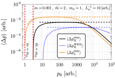
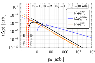
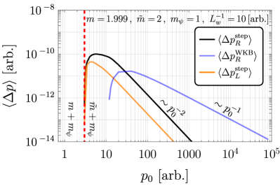
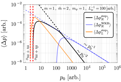
Figure 5: We present here numerical results for the averaged momentum transfer to the wall for each of the three contributions in eq. (2.7) as a function of incoming particle energy. Black and orange curves stand for right and left emission of soft quanta (using step wall), while blue for the energetic quanta (using WKB). The vertical red dashed lines are the lower bounds on the minimal energy the incoming particle can have to emit right and left modes. We show four cases of interest, that respectively are: $\tilde{m}\gg m$, $\tilde{m}\sim O(1)m$, $\tilde{m}-m\ll 1$ and $L_{w}^{-1}\gg\tilde{m}$. The horizontal and oblique dashed lines are analytical estimates in eq. 51 ($\langle{\Delta p^{\rm wkb}_{\zeta_{R}}}\rangle$), in eq. 207 ($\langle{\Delta p^{\rm step}_{\zeta_{L}}}\rangle$) and in eq. 208 ($\langle{\Delta p^{\rm step}_{\zeta_{R}}}\rangle$). At the highest scales the WKB contribution always dominates and falls as $p_{0}^{-1}$ (while both step wall contributions fall as $p_{0}^{-2}$). In the limit $L_{w}\rightarrow 0$, $R$ emission also falls off as $p_{0}^{-1}$. Most interestingly, for large hierarchy $m_{\psi}/m$, $\langle{\Delta p}\rangle$ is constant until $p_{0}\lesssim\tilde{m}m_{\psi}/m$.

2.9 Pressure from scalar emission

We now come to finally computing the pressure induced on the bubble wall from scalar emission calculated above. We will discover that in the case of $m\ll\tilde{m}$, this can be sizable. In order to find the pressure acting on the bubble wall we need to perform the integration over the flux of incoming particles

$${\cal P}=\int\frac{d^{3}p}{(2\pi)^{3}}f_{\psi}(T,\gamma_{w})\times\frac{p^{z}}{p_{0}}\langle{\Delta p^{\rm total}}\rangle.$$ (53)

We will focus on the cases displaying a constant behaviour for the exchange of momentum, that we call plateau for $p_{0}<\tilde{m}m_{\psi}/m$. If the average momentum transfer is a constant the integration is simple and we find

$${\cal P}^{\rm scalar}=n_{\psi}(T,\gamma_{w})\langle{\Delta p^{\rm total}}\rangle=\gamma_{w}n_{\psi}(T)\langle{\Delta p^{\rm total}}\rangle,\qquad p_{0}<\frac{\tilde{m}m_{\psi}}{m},$$ (54)

in the ultrarelativistic case $p^{z}/p_{0}\to 1$. To go from the second equality to the third, we used that in the wall frame, the plasma frame thermal distribution of $\psi$, $n_{\psi}(T)$ is boosted. Summing all of the contributions and using eq. 52, we find

$${\cal P}^{\rm scalar}\approx\begin{cases}\frac{\zeta(3)\gamma_{w}T^{3}}{8\pi^{4}}{y^{2}\tilde{m}\over m_{\psi}^{2}}\times\gamma_{w}\qquad\gamma_{w}<\frac{\tilde{m}m_{\psi}}{mT}\\ \frac{\zeta(3)T^{2}}{8\pi^{4}}{y^{2}\tilde{m}^{2}\over m_{\psi}m}\qquad\gamma_{w}>\frac{\tilde{m}m_{\psi}}{mT}\end{cases}$$ (55)

We observe that this contribution becomes relevant and dominates over the LO contribution if ${y^{2}\over 8\pi^{2}m_{\psi}m}>1$.

We remind however the reader that this result for the pressure was obtained for a particular choice of interactions in the Lagrangian eq. 5 and parameters. We have chosen these couplings in order to mimic as much as possible the vector radiation from the current to be discussed in the next section. Whether the pressure contribution in eq. 55 can be phenomenologically relevant is left for further studies.

3 Spontaneously broken gauge theories

We now proceed to the phase transitions related to the spontaneous breaking of the gauge symmetries and the emission of the vector bosons. The procedure will in essence be exactly the same as what we presented for the case of the scalar emission. We will quantise the theory of a gauge field in the background of a domain wall interpolating between a symmetric and broken phase. As should be expected, the extra difficulty will involve dealing with gauge-fixing and the change of degrees of freedom due to the spatially-dependent rearrangement of the vacuum.

For simplicity, we will consider the Abelian Higgs model of a charged complex scalar $H$, whose potential $V(H)$ is responsible for spontaneous breaking of the $U(1)$ gauge symmetry. A second scalar field $\psi$ charged under the same $U(1)$ will play of the role of matter; its potential is trivial. The Lagrangian is

$$\begin{split}\mathcal{L}&=-\frac{1}{4}F_{\mu\nu}F^{\mu\nu}+|D_{\mu}H|^{2}-V(\sqrt{2}|H|)+|D_{\mu}\psi|^{2}-m_{\psi}^{2}|\psi|^{2},\end{split}$$ (56)

where we are using the convention $D_{\mu}\psi=(\partial_{\mu}+igA_{\mu})\psi$ and $A_{\mu}$ is the vector gauge field. We will in general not need commit to a specific potential but will simply assume that it has two minima at $\sqrt{2}|H|=v,\tilde{v}$, where $v=0$ corresponds to the symmetric phase. We will quantise the theory in the background of a domain wall $\sqrt{2}\langle|H|\rangle=v(z)$. We will also be interested, both as a computational tool and as a phenomenological case in its own right, in imagining a distorted or more general class of potential with non-zero $v<\tilde{v}$. We will call this scenario a broken to broken phase transition, in opposition to the usual case of symmetric to broken phase transitions.

To work with the theory described by eq. 56, one has to make two independent choices: what field coordinates to use for $H$, such as Cartesian or polar, and what gauge to impose. The value of each choice is determined by the particular application. Much of the following pages will be dedicated to arguing for the most convenient choices for our application.

If we are interested in studying the geometry of the vacuum manifold, polar coordinates $H={1\over\sqrt{2}}(h+v)e^{i{\chi\over v}}$ are most convenient. The potential depends only on the modulus. In the symmetric phase however this coordinate choice is singular. On the other, Cartesian coordinates are well-defined everywhere

$$H={1\over\sqrt{2}}(h_{1}+ih_{2})\equiv{1\over\sqrt{2}}(h+v+ih_{2})\ ,$$ (57)

where we have expanded around the background solution $v=v(z)$. The Lagrangian for the Higgs and gauge fields becomes

$$\begin{split}\mathcal{L}_{A,H}&=-{1\over 4}F_{\mu\nu}F^{\mu\nu}+\frac{1}{2}(\partial h)^{2}+\frac{1}{2}(\partial h_{2})^{2}\\ &\quad-gA^{\mu}\left[h_{2}\partial_{\mu}v(z)-v(z)\partial_{\mu}h_{2}\right]+{1\over 2}g^{2}v^{2}(z)A^{2}-\frac{1}{2}\partial_{1}^{2}V(v(z))h^{2}-\frac{1}{2}\partial_{2}^{2}V(v(z))h_{2}^{2}+\dots\ ,\end{split}$$ (58)

up to quadratic terms, where $\partial_{i}\equiv\partial/\partial h_{i}$, so that the last two terms are the $z$-dependent mass terms of $h_{1,2}$.

At a non-zero minimum of the potential, $h_{2}$ becomes massless and is the would-be Goldstone boson. As always for gauge theories, when $v\neq 0$ a mixing term appears between this goldstone boson and the gauge boson. However, in the context of a varying background, there is also an extra mixing proportional to $\partial_{z}v$. When $v$ is a constant, the mixing can be eliminated completely while also gauge fixing by adding the so called $R_{\xi}$ gauge term

$$\delta\mathcal{L}_{g.f.}=-{1\over 2\xi}(\partial_{\mu}A^{\mu}-\xi gvh_{2})^{2}\ ,$$ (59)

and integrating by parts. For $v=v(z)$, adding this same (now $z-$dependent) gauge-fixing term does not get rid of mixing entirely but localises it to the region of the wall

$$\begin{split}\mathcal{L}_{A,H}+\delta\mathcal{L}_{g.f.}=&-{1\over 4}F_{\mu\nu}F^{\mu\nu}-{1\over 2\xi}(\partial_{\mu}A^{\mu})^{2}+\frac{1}{2}(\partial h)^{2}+\frac{1}{2}(\partial h_{2})^{2}\\ &-2gh_{2}A^{z}\partial_{z}v(z)+{1\over 2}g^{2}v(z)^{2}A^{2}-\frac{1}{2}\partial_{1}^{2}V(v(z))h^{2}\\ &-\frac{1}{2}\left[\partial_{2}^{2}V(v(z))+\xi g^{2}v^{2}(z)\right]h_{2}^{2}+\dots\ .\end{split}$$ (60)

3.1 Particle content in the asymptotic regions

We briefly remind ourselves of the spectrum of the theory in the asymptotic regions $v=0$ and $\tilde{v}$ at $z\rightarrow-\infty$ and $z\rightarrow\infty$ respectively, before discussing the full interpolating space.

Symmetric phase:

The theory eq. 60 around the symmetric point minimum $v=0$ describes two scalars $h_{1,2,}$ with equal mass by symmetry

$$m_{h,s}^{2}\equiv\partial_{1}^{2}V(0)=\partial_{2}^{2}V(0)$$ (61)

The gauge-fixing affects only the Maxwell equations of motion for the massless vector $A^{\mu}$. Whatever the value of $\xi$, we identify two physical degrees of freedom with polarisation vectors given by

$$\epsilon^{\mu}_{T_{1}}=(0,0,1,0)\ ,\qquad\epsilon^{\mu}_{T_{2}}=\frac{1}{\sqrt{k_{\perp}^{2}+k_{z}^{2}}}(0,k^{z},0,-k_{\perp})\ ,$$ (62)

for $k^{\mu}=(k_{0},k_{\perp},0,k^{z})$. The only subtlety is one has to impose constraints on the physical states, the Gupta-Bleuler condition.

Broken phase(s):

At a symmetry breaking minimum $\partial_{2}^{2}V(\tilde{v})=0$ and $h_{2}$ describes the would-be NGB. A particularly convenient choice is the ‘unitary gauge’, corresponding to $\xi\rightarrow\infty$ in which the the NGB decouples completely making manifest the spectrum. We are left with a single massive scalar (the Higgs) $h$ with mass squared equal to $\partial_{1}^{2}V(\tilde{v})$ and a massive vector boson $A_{\mu}$ with mass

$$\tilde{m}\equiv g\tilde{v}\ ,$$ (63)

and satisfying the Proca equation, which reduced to a Klein-Gordon equation for each component of $A^{\mu}$ supplemented by the Lorentz condition.

$$\partial_{\mu}F^{\mu\nu}+\tilde{m}^{2}A^{\nu}=0\ ,$$ (64)

$$\implies\; \partial^{2}A^{\mu}+\tilde{m}^{2}A^{\mu}=0\ ,\qquad\partial_{\mu}A^{\mu}=0\ .$$ (65)

Solving this is straightforward and one adds to the transverse polarisations of eq. 62 a third longitudinal one parallel to $3-$momentum

$$\begin{split}\epsilon_{L}^{\mu}=\left(\frac{p_{0}^{2}-m^{2}}{p_{0}},p_{\perp},0,p^{z}\right)\frac{p_{0}}{m\sqrt{p_{0}^{2}-m^{2}}}.\end{split}$$ (66)

3.2 Global degrees of freedom

Here will analyse the fields defined over the entire region and identify the appropriate global modes to quantise, where by global we simply mean they are good across the wall.

In principle, one could choose a convenient value of $\xi$ in eq. 60 and push ahead with quantisation. However, we would have to deal with mixing when solving for the mode functions as well as take care to impose a Gupta-Bleuler like condition on the physical states. Luckily, we will argue that even when asymptotically approaching the symmetric point as $z\rightarrow-\infty$, it is possible to work with unitary gauge $\xi\rightarrow\infty$ with impunity. This approach was already made at the classical level in ref.[70], and we will re-derive and tweak some of their results using a slightly different language, before quantising.

In unitary gauge the $h_{2}$ degree of freedom decouples and the theory becomes

$$\begin{split}\mathcal{L}^{U.G.}_{A,H}=&-{1\over 4}F_{\mu\nu}F^{\mu\nu}+{1\over 2}g^{2}v^{2}(z)A^{2}+\frac{1}{2}(\partial h)^{2}-\frac{1}{2}\partial_{1}^{2}V(v)h^{2}+\dots\ ,\end{split}$$ (67)

and the equations of motion for eq. 58 reduce to just two uncoupled equations

$$\Box h=-V^{\prime\prime}(v)h\,,$$ (68)

$$\partial_{\nu}F^{\mu\nu}=g^{2}v^{2}(z)A^{\mu}\,.$$ (69)

The first one is the equation of motion for the physical Higgs boson $h$ and we will not have anymore to say about it. The second will be the focus of our attention. While $v(z)>0$, the theory is always in a broken phase and $A^{\mu}$ describes a massive vector. Unitary gauge is then manifestly a valid choice. Note that the usual transversality condition for massive vector bosons in this case becomes

$$\partial_{\mu}\partial_{\nu}F^{\mu\nu}=\partial_{\mu}(g^{2}v^{2}A^{\mu})=0\,,$$ (70)

$$\implies\partial_{n}A^{n}+\partial_{z}A^{z}=-{\partial_{z}v^{2}\over v^{2}}A^{z}\ ,$$ (71)

which, in the presence of the bubble, generalises the standard Lorentz condition $\partial_{\mu}A^{\mu}=0$ for massive electrodynamics. The constraint above ensures this vector field has three polarisation degrees of freedom. Subbing this back into eq. 69 we get

$$\partial^{2}A^{\mu}+\partial^{\mu}\left[\left(\partial_{z}v^{2}\over v^{2}\right)A^{z}\right]+g^{2}v^{2}A^{\mu}=0\ .$$ (72)

The general Fourier mode can be written as

$$A^{\mu}_{k_{0},k_{\perp}}=e^{-ik_{n}x^{n}}\sum_{l}a_{l}\;\chi_{l,k^{n}}^{\mu}(z)\,,$$ (73)

where $l$ runs over three indices, $a_{l}$ are some constant Fourier coefficients and the functions $\chi_{l,k_{0},k_{\perp}}^{\mu}(z)$ have to be found by solving eq. 72.

$\tau$ polarisations:

It is useful to define what we call $\tau-$polarisations by the condition $A^{z}=0$, since for these we recover the Lorentz condition $\partial_{\mu}A^{\mu}=0$, which in Fourier space reduces to

$$k_{n}\chi_{\tau}^{n}\equiv k_{0}\chi^{0}_{\tau}-k_{\perp}\chi^{\perp}_{\tau}=0\ ,$$ (74)

and has solutions in terms of two constant vectors

$$\chi_{\tau}^{\mu} =\epsilon_{\tau_{1,2}}^{\mu}\;\chi_{\tau_{1,2}}(z)\ ,$$ (75)

where

$$\epsilon_{\tau_{1}}^{\mu}= (0,0,1,0),\qquad\epsilon_{\tau_{2}}^{\mu}=(k_{\perp},k_{0},0,0)/\sqrt{k_{0}^{2}-k_{\perp}^{2}}\ ,$$ (76)

and the equations of motion eq. 72 become the Klein-Gordon-like

$$\left[E^{2}-\partial_{z}^{2}+g^{2}v^{2}(z)\right]\chi_{\tau_{1,2}}(z)=0\ ,$$ (77)

where we remind the reader of the definition $E=\sqrt{k_{0}^{2}-k_{\perp}^{2}}$. Note that $\epsilon_{\tau_{1}}^{\mu}$ is one of the standard transverse polarisations, but $\epsilon_{\tau_{2}}$ is not, since it has non-zero time component, and is not orthogonal to three momentum. The wave equation to solve across the wall for $\tau$ d.o.f. is thus identical to the scalar case studied in section 2.

$\lambda$ polarisation:

It remains to solve for the remaining degree of freedom with $A^{z}\neq 0$. The wave equation to solve for $A^{z}$ is obtained by setting $\mu=z$ in eq. 72. We will analyse it more in the next section but we note that it is significantly more complicated than what we found for the $\tau$ d.o.f.. Whatever the solution, the other components of the vector are fixed. Requiring orthogonality with $\chi_{\tau}^{\mu}$ implies the form $\chi_{\lambda}^{\mu}(z)=\left(-ik^{n}\alpha(z),\chi^{z}_{\lambda}\right)$ where $n=0,\perp$. The generalised Lorentz condition in eq. 71 immediately leads to the relation

$$\alpha(z)={\partial_{z}\left(v^{2}\chi^{z}_{\lambda}\right)\over E^{2}\;v^{2}}.$$ (78)

Plugging this back into the eq. 72 we obtain the equation in terms of the $\chi^{z}$ only

$$-E^{2}\chi^{z}_{\lambda}-\partial_{z}\left(\frac{1}{v^{2}}\partial_{z}(v^{2}\chi^{z}_{\lambda})\right)+g^{2}v^{2}(z)\chi^{z}_{\lambda}=0.$$ (79)

We can get rid of the linear in derivative term if we introduce a new function $\lambda(z)$

$$\chi_{\lambda}^{z}={E\over{gv(z)}}\lambda(z)$$ (80)

and eq. (79) becomes Schrodinger-like

$$\left(-E^{2}-\partial_{z}^{2}+U_{\lambda}(z)\right)\lambda=0.$$ (81)

with effective potential

$$\begin{split}U_{\lambda}(z)=&\;g^{2}v^{2}(z)-v\;\partial_{z}\left(\partial_{z}v\over v^{2}\right)\\ =&\;g^{2}v^{2}(z)+2\left(\partial_{z}v\over v\right)^{2}-{\partial_{z}^{2}v\over v}.\end{split}$$ (82)

Note that the solutions in terms of $\lambda$ function unlike $\chi_{\lambda}^{z}$ will satisfy the usual orthogonality relations

$$\int dz\lambda_{k}(z)\lambda_{q}^{*}(z)=2\pi\delta(k^{z}-q^{z})$$ (83)

It is easy to prove $-$ and we do so explicitly in appendix D $-$ that for an interpolating solution $v(z)$ of a completely arbitrary Higgs potential $V$, we have $(v^{\prime}/v)^{2},v^{\prime\prime}/v\rightarrow m_{h,s}^{2}$ as $z\rightarrow-\infty$ so that $U_{\lambda}(z)$ is always finite even if $v=0$ and more precisely

$$\lim\limits_{z\to-\infty}U_{\lambda}(z)=\begin{cases}g^{2}v^{2}\ ,&v\neq 0\\ m_{h,s}^{2}\ ,&v=0\end{cases}\ \equiv m_{\lambda}^{2}\ .$$ (84)

We see that $\lambda$ is the perfect cross-wall field. It interpolates between one of the massive (Higgs) degrees of freedom on the symmetric $v=0$ side $z\rightarrow-\infty$ and a third component of the massive vector in the broken region $z\rightarrow\infty$. If instead $v\neq 0$, $\lambda$ simply interpolates between the different mass vectors.

Let us look at the $A_{\mu}$ vector formed by the $\lambda$ field. In general we need to solve the equations of motion, however even without a complete solution $z$ component of eq. 69 forces the relations on-shell:

$$\chi^{z}_{\lambda} = \frac{E^{2}\partial_{z}\alpha}{E^{2}-g^{2}v^{2}(z)}\Rightarrow$$

$$\chi_{\lambda}^{\mu} = \left(-ik^{n}\alpha(z),\chi_{\lambda}^{z}\right)=(-ik^{n},\partial^{z})\;\alpha(z)+{g^{2}v^{2}(z)\over E^{2}}\chi_{\lambda}^{z}(0,0,0,1)$$ (85)

$$= (-ik^{n},\partial^{z})\;\alpha(z)+{gv(z)\over E}\lambda(z)(0,0,0,1)$$

So that the total vector can be written as a complete derivative plus a term sub-leading in energy. This expansion turns out to be very useful in calculating the amplitudes for the physical processes. Far from the wall when $v\to const$ we can introduce the polarisation vectors $\epsilon_{\lambda}^{\mu}$ such that

$$\chi_{\lambda}^{\mu} \propto \epsilon_{\lambda}^{\mu},~{}~{}~{}\epsilon^{\lambda}_{\mu}\epsilon^{\lambda^{\mu}}=-1$$

$$\epsilon_{\lambda}^{\mu} = \left(k^{n}{k^{z}\over E^{2}}\ ,1\right)\times\frac{E}{gv}$$ (86)

$$= {k^{z}\over Egv}\;k^{\mu}+{gv\over E}(0\ ,0\ ,0\ ,1)\ ,$$

We would like to emphasise that these $\lambda$ and $\tau$ differ from the conventional transverse and longitudinal polarisations. In the case of no domain wall all three polarisations satisfy the same equations of motion and one can use any linear combination of them as a basis to decompose the vector field. Outside of the wall we can relate $\tau,\lambda$ to the longitudinal and transverse polarisations

$$\epsilon_{T_{1}}=(0,0,1,0)$$

$$\epsilon_{T_{2}}=\frac{1}{\sqrt{k_{0}^{2}-m^{2}}}(0,k^{z},0,-k_{\perp})$$

$$\epsilon_{L}=\left(\frac{k_{0}^{2}-m^{2}}{k_{0}},k_{\perp},0,k^{z}\right)\frac{k_{0}}{m\sqrt{k_{0}^{2}-m^{2}}}$$

and two basis of polarisations are related by the rotation matrix

$$\left(\begin{array}[]{c}\epsilon_{T_{1}}\\ \epsilon_{T_{2}}\\ \epsilon_{L}\end{array}\right)=\left(\begin{array}[]{ccc}1&0&0\\ 0&\frac{k_{0}k^{z}}{E\sqrt{k_{0}^{2}-m^{2}}}&-\frac{k_{\perp}m}{E\sqrt{k_{0}^{2}-m^{2}}}\\ 0&\frac{k_{\perp}m}{E\sqrt{k_{0}^{2}-m^{2}}}&\frac{k_{0}k^{z}}{E\sqrt{k_{0}^{2}-m^{2}}}\\ \end{array}\right)\left(\begin{array}[]{c}\epsilon_{\tau_{1}}\\ \epsilon_{\tau_{2}}\\ \epsilon_{\lambda}\end{array}\right)$$ (97)

In the case of a very large $k^{z},E\gg k_{\perp},m$ the mixing angle between $\tau,\lambda$ transverse and longitudinals scales as $m/E$. We can see that two basis of polarisations are exactly the same for the case $k_{\perp}=0$. This is expected since for this configuration of momenta $T_{1},T_{2}$ polarisations have zero component in $z$ direction. Using the unbroken part of the Lorentz symmetry (boosts in $x-y$ direction) we can obtain the polarisations for generic momenta, which indeed agrees with $\tau,\lambda$ basis derived before. Our goal in this paper is to calculate the total pressure acting on the domain wall and for this calculation we need to sum the contributions from of all polarisations. At this point we can perform all of the calculations in the $\tau,\lambda$ basis, without even reporting the results for $T,L$ polarisations.

Figure 6: The potential for the $\lambda$ degree of freedom, which is defined everywhere. Recall $m=gv$ and $\tilde{m}=g\tilde{v}$, plus thermal corrections. As $v\rightarrow 0$ a growing plateau develops ending at $z\sim m_{h,s}^{-1}\ln\left(v/\tilde{v}\right)$ with value $m_{h,s}^{2}$ - the symmetric side mass of the Higgs in the case $v=0$ exactly. These curves were drawn using the explicit profile eq. 103.

3.2.1 $v\to 0$ limit

All of the previous discussion applied most manifestly for the case when the vev of the symmetry breaking field is $v\neq 0$. What will happen in the case when the domain wall separates the vacua where in one of the the gauge symmetry is unbroken? We have seen in the previous section that the potential of the $\lambda$ mode has a property that in $v\to 0,U_{\lambda}(z)\to m_{h,s}^{2}$, which together with our expectations from the Higgs phenomena hints that $\lambda$ mode on the unbroken side should correspond to the would be Goldstone boson

$$\lambda_{z\to-\infty}\to h_{2}\,.$$ (98)

To understand this matching better let us look at the $\chi^{\mu}_{\lambda}$ vector in the limit $v\to 0$

$$\chi^{\mu}_{\lambda} = \left(-ik^{n}\alpha(z),\chi_{\lambda}^{z}\right)=\left(\frac{-ik^{n}\partial_{z}(v\lambda)}{gEv^{2}},\frac{E}{gv}\lambda\right)$$ (99)

$$= \frac{\lambda}{gv}\left(-\frac{ik^{n}}{E}\left[\frac{v^{\prime}}{v}+\frac{\lambda^{\prime}}{\lambda}\right],E\right)_{v\to 0}=\frac{e^{-ikx}}{gv}\left(\frac{k^{n}}{E}\left[-im_{h,s}+k^{z}\right],E\right),$$

where we have used that $\lambda$ becomes a plane wave far from the wall and $v^{\prime}/v\to m_{h,s}$. Note that the factor $(-im_{h,s}+k^{z})/E$ is a pure phase if the $\lambda$ dof is on shell. Let us see whether we can build exactly the same vector but from the Goldstone fields $h_{2}$. Indeed if we consider the vector

$$\partial^{\mu}\left(\frac{h_{2}}{gv}\right)=-\frac{e^{-ikx}}{gv}\left(k^{n},k^{z}+i\frac{v^{\prime}}{v}\right)=\frac{-iEe^{-ikx}}{gv(k^{z}-im_{h,s})}\left(\frac{k^{n}}{E}\left[-im_{h,s}+k^{z}\right],E\right).$$ (100)

So we can see, comparing with eq. 99, that the two vectors $\chi_{\lambda}^{\mu}$ and $\partial_{\mu}(h_{2}/gv)$ are exactly the same apart from the constant phase factor, so indeed $\lambda$ field in the $z\to-\infty$ limit corresponds to the Goldstone boson.

What about starting from a finite value and taking $v\rightarrow 0$? For concreteness let us consider the potential

$$V=\lambda_{h}(|h|-v)^{2}(|h|-\tilde{v})^{2}.$$ (101)

First of all the potential has a cusp at $|h|=0$ so the limit $v\to 0$ becomes discontinuous. This can be seen also by the form of $U_{\lambda}(z)$. As $v$ becomes smaller a longer finite plateau develops in the potential with value $\approx m_{h,s}^{2}$, as is shown in fig. 6. No matter how small $v$ eventually the potential turns down and asymptotes to $g^{2}v^{2}$ as is to be expected. Thus for any finite though tiny $v$ the asymptotic states at $z\rightarrow-\infty$ are those of a massive vector.

3.3 The step wall case

In order to proceed further we need to solve the equations of motion. In general it is a complicated problem depending on the shape of the potential. One needs to find the solitonic solution $v(z)$ connecting false and true vacuum and later the wavemodes describing perturbations of each field on this background. In the particular case of the domain wall

$$v(z)=\frac{1}{2}\tilde{v}\left(1+\tanh\left(z\over L_{w}\right)\right)\ ,$$ (102)

the solutions were found in [70] in terms of hypergeometric functions. In this paper we will consider an even simpler case, namely a step function ansatz for the wall. This approximation will of course be valid only if the momentum of the particle during the passage is (much) less than inverse width of the wall $k,\tilde{k}\ll L_{w}^{-1}$. Typically, this width is controlled by the mass of the Higgs $L_{w}^{-1}\approx m_{h}$.

The solution of the equations of motion can be written down on each side immediately and the only challenge becomes deriving and implementing matching conditions. In this section we report the matching conditions for $\tau$ and $\lambda$ polarisations and write down the corresponding wave functions. We will do so first for the broken to broken case $v>0$. As an explicit example we can imagine distorting eq. 102 to

$$v(z)\rightarrow v+\frac{1}{2}\left(\tilde{v}-v\right)\left(1+\tanh\left(z\over L_{w}\right)\right)\ .$$ (103)

We then comment on the $v\rightarrow 0$ limit, which is straightforward for $\tau$ degrees of freedom but more delicate for $\lambda$.

3.3.1 $(\tau)$ polarisations

For the $\tau$ polarisations, we showed in section 3.2 that the equations of motion are exactly the same as for the scalar field $(\Box A^{\mu}_{(\tau)}=-g^{2}v^{2}A^{\mu}_{(\tau)})$ and so for the step wall the matching conditions become:

$$\chi_{\tau_{i}}|_{<0} =\chi_{\tau_{i}}|_{>0}\ ,$$ (104)

$$\partial_{z}\chi_{\tau_{i}}|_{<0} =\partial_{z}\chi_{\tau_{i}}|_{>0}\ ,$$ (105)

with $i=1,2$. The reflection and transmission coefficients are thus the same as for scalars and the wave functions become

$$\chi_{\tau_{i},R,k}^{\mu}(z) =\epsilon_{\tau_{i}}^{\mu}\begin{cases}e^{ik^{z}z}+r^{\tau}_{k}e^{-ik^{z}z}\ ,&z<0\\ t^{\tau}_{k}\;e^{i\tilde{k}^{z}z}\ ,&z>0\end{cases}$$ (106)

$$\chi_{\tau_{i},L,k}^{\mu}(z) =\epsilon_{\tau_{i}}^{\mu}\sqrt{k^{z}\over\tilde{k}^{z}}\begin{cases}\frac{\tilde{k}^{z}}{k^{z}}t^{\tau}_{k}\;e^{-ik^{z}z}\ ,&z<0\\ e^{-i\tilde{k}^{z}z}-r^{\tau}_{k}e^{i\tilde{k}^{z}z}\ ,&z>0\end{cases}$$ (107)

where

$$r^{\tau}_{k} =\frac{k^{z}-\tilde{k}^{z}}{k^{z}+\tilde{k}^{z}}\ ,~{}~{}~{}t^{\tau}_{k}=\frac{2k^{z}}{k^{z}+\tilde{k}^{z}}\ ,$$ (108)

$$k_{0} =\sqrt{k_{z}^{2}+m^{2}+k_{\perp}^{2}}\ ,\quad\tilde{k}^{z}=\sqrt{k_{0}^{2}-\tilde{m}^{2}-k_{\perp}^{2}}\ ,\quad m\equiv gv\ ,\quad\tilde{m}\equiv g\tilde{v}\ .$$

Taking the $v\rightarrow 0$ limit for these degrees of freedom is simple and we approach the $v=0$ case smoothly.

3.3.2 $(\lambda)$ polarisation

The $\lambda$ modes require more work. Again we first focus on the broken to broken case of $v>0$. Matching conditions are easy to derive by integrating the wave equation for $\lambda$ once and twice respectively (most easily done at the level of eq. 79). These are

$$\left.{\partial_{z}\lambda\over v(z)}\right|_{<0} =\left.\partial_{z}\lambda\over v(z)\right|_{>0}\ ,$$

$$\left.v(z)\lambda\right|_{<0} =\left.v(z)\lambda\right|_{>0}\ ,$$ (109)

which allows us to write down the expressions for (in-state) ‘left’ and ‘right’ movers:

$$\lambda_{R,k}(z) =\begin{cases}e^{ik^{z}z}+r^{\lambda}_{k}e^{-ik^{z}z}\ ,&z<0\\ t^{\lambda}_{k}\;e^{i\tilde{k}^{z}z}\ ,&z>0\end{cases}$$ (110)

$$\lambda_{L,k}(z) =\sqrt{k^{z}\over\tilde{k}^{z}}\begin{cases}\frac{\tilde{k^{z}}}{k^{z}}t^{\lambda}_{k}e^{-ik^{z}z}\ ,&z<0\\ e^{-i\tilde{k}^{z}z}-r^{\lambda}_{k}e^{i\tilde{k}^{z}z}\ ,&z>0\end{cases}$$ (111)

where

$$r^{\lambda}_{k} =\frac{\tilde{v}^{2}k^{z}-v^{2}\tilde{k}^{z}}{\tilde{v}^{2}k^{z}+v^{2}\tilde{k}^{z}}\ ,\quad t^{\lambda}_{k}=\frac{2k^{z}v\tilde{v}}{\tilde{v}^{2}k^{z}+v^{2}\tilde{k}^{z}}\ ,$$ (112)

$$k_{0} =\sqrt{k_{z}^{2}+m^{2}+k_{\perp}^{2}}\ ,\quad\tilde{k}^{z}=\sqrt{k_{0}^{2}-\tilde{m}^{2}-k_{\perp}^{2}}\ ,\quad m\equiv gv\ ,\quad\tilde{m}\equiv g\tilde{v}\ .$$

Notice that in the relativistic limit

$$r^{\lambda}_{k}\rightarrow{\tilde{v}^{2}-v^{2}\over\tilde{v}^{2}+v^{2}}\ ,\qquad\text{for}\quad k^{z}\gg m,\tilde{m}\ .$$ (113)

so that $\lambda$ maintains a finite reflection probability as long as the step function is a valid approximation, as was pointed out in [68].

Interestingly we can see that $r^{\lambda}_{k}\to 1$ in the limit $v\to 0$, i.e. the wall becomes completely non-transparent for the $\lambda$ polarisations in this limit (step wall $\cup\ v\to 0\cup k^{z}\gg m,\tilde{m}$). This in-penetrability of the wall deserves some discussion. It becomes more clear if we consider the explicit form of $U_{\lambda}(z)$ for the case of the $tanh$ profile of the wall (see eq. 103). As was mentioned in the section 3.2.1 and is sketched in fig. 6, in the limit of $v\rightarrow 0$, $U_{\lambda}(z)$ develops a growing plateau with a height $\approx L_{w}^{-2}\sim m_{h,s}^{2}$ and width $L_{\rm plateau}\sim L_{w}\log\tilde{v}/v$. In the step function approximation both these scales are sent to infinity. For $v=0$ exactly then there are no oscillating $\lambda_{R,k}$ modes at all in the step approximation, while $\lambda_{L,k}$ are completely reflected. For $v$ tiny but non-zero the potential eventually does instead relax to $m^{2}$ and both oscillating $\lambda_{L,R}$ solutions exist, but are constrained to live on opposite sides of the wall.

A comment on bound states:

We have so far considered ‘scattering state’ solutions to the equations of motion, i.e. those which are plane waves far from the wall. What about bound states? In principle such states are possible for $\lambda$ polarisation. Ref[70] found that there is one for the case when $v=0$ and the potential satisfies some specific constraints. Examining the form of the potential for $v>0$ in 6 it appears that a bound state might generically appear. The mass of these bound states is controlled by the scale $L_{w}^{-1}$ as is obvious by absence of the bound state in the step wall limit. One could in principle calculate in the WKB limit the amplitude for an incoming particle to excite this bound state. We leave this interesting exercise to future work.

3.4 Quantisation

Summarising the previous sections, we can expand the field into a complete basis of eigenmodes of the free theory in the background vev $v(z)$,

$$\begin{split}A^{\mu}&=\sum_{I,\ell}\int\frac{d^{3}k}{(2\pi)^{3}\sqrt{2k_{0}}}e^{-i(k_{0}t-\vec{k}_{\perp}\vec{x})}\left(a^{\rm in}_{\ell,I,k}\;\chi_{\ell,I,k}^{\mu}(z)+h.c.\right)\\ &=\sum_{I,\ell}\int\frac{d^{3}k}{(2\pi)^{3}\sqrt{2k_{0}}}e^{-i(k_{0}t-\vec{k}_{\perp}\vec{x})}\left(a^{\rm out}_{\ell,I,k}\;\zeta_{\ell,I,k}^{\mu}(z)+h.c.\right)\ ,\end{split}$$ (114)

where $I=R,L$ denote right and left movers, $\ell=\tau_{1},\tau_{2},\lambda$ sums over different polarisations. The wave modes $\chi^{\mu}(z)$ are in general constructed via

$$\chi_{\tau_{i},I,k}^{\mu} =\epsilon_{\tau_{i}}^{\mu}\;\chi_{\tau_{i},I,k}(z)\ ,$$ (115)

$$\chi_{\lambda,I,k}^{\mu} =\left(\frac{-ik^{n}\partial_{z}(v\lambda_{I,k})}{gEv^{2}},\frac{E}{gv}\lambda_{I,k}\right)\overset{\rm on\ shell}{=}\bar{\partial}^{\mu}\left({\partial_{z}\left(v\lambda_{I,k}^{z}\right)\over Eg\;v^{2}}\right)+{gv(z)\over E}\lambda_{I,k}\;\delta^{\mu}_{z}\ ,$$ (116)

where $\bar{\partial^{\mu}}\equiv(-ik^{n},\partial^{z})$, with the explicit form of scalar fields $\chi_{\tau_{i},I,k}(z)$ and $\lambda_{I,k}(z)$ obtained by solving the respective Schrodinger-like wave eqs. 77 and 81 with appropriate $R,L$-mover boundary conditions. In the step wall approximation for the vev $v(z)$, these are given analytically in eqs. 106, 107, 110 and 111. In complete analogy to the case of fundamental scalars, the modes $\chi_{\ell,I,k}^{\mu}$ should be thought of as describing incoming (early time) eigenstates of momentum (particles) in the plane wave limit with physical $z-$momentum $k^{z}>0$ and $-k^{z}$ for $R$ and $L$ respectively. Modes describing outgoing (late time) eigenstates of momenta $\zeta_{\ell,I,k}^{\mu}$ are instead obtained via

$$\zeta_{\tau_{i},\{L,R\}}^{\mu} =\epsilon_{\tau_{i}}^{\mu}\;\chi^{*}_{\tau_{i},\{R,L\}}(z),\qquad$$ (117)

$$\zeta_{\lambda,\{L,R\}}^{\mu} =\left(\frac{-ik^{n}\partial_{z}(v\lambda^{*}_{\{R,L\}})}{gEv^{2}},\frac{E}{gv}\lambda^{*}_{\{R,L\}}\right)\overset{\rm on\ shell}{=}\bar{\partial}^{\mu}\left({\partial_{z}(v\lambda_{\{R,L\}}^{*})\over Eg\;v^{2}}\right)+{gv(z)\over E}\lambda_{\{R,L\}}^{*}\;\delta^{\mu}_{z}\ ,$$ (118)

where we have dropped $k$ labels to not clutter the notation. Notice the switch in $L,R$ - labels. Both sets of eigenmodes form a complete orthonormal basis and can be used to expand the field operator in eq. 114. The associated Fourier operators carry $\rm in$ and $\rm out$ labels to emphasise that they create / annihilate in and out states in the $S-$matrix language

$$\left|k^{\rm in}_{\ell,I}\right\rangle \equiv\sqrt{2k_{0}}\;(a_{\ell,I,k}^{\rm in})^{\dagger}\left|0\right\rangle\ ,$$ (119)

$$\left|k^{\rm out}_{\ell,I}\right\rangle \equiv\sqrt{2k_{0}}\;(a_{\ell,I,k}^{\rm out})^{\dagger}\left|0\right\rangle\ ,\qquad I\in R,L\quad\&\quad\ell\in\tau_{1},\tau_{2},\lambda\ .$$ (120)

Both satisfy the usual algebra eq. 19 upon quantisation.

Ward identity and current conservation:

We now comment on current conservation in the case of spontaneously broken Lorentz symmetry. If the gauge symmetry is preserved, vector bosons can couple only to conserved currents. This is not the case when it is spontaneously broken, but we may still choose to consider coupling to a conserved current . In the Lorentz invariant theory the statement of the current conservation can be expressed in terms of amplitudes. Given an arbitrary process with an external vector leg with momentum $k^{\mu}$, we have the following identity

$$\mathcal{M}^{(4,J)}\equiv\epsilon_{k}^{\mu}\mathcal{M}^{(4,J)}_{\mu}=(\epsilon_{k}^{\mu}+{k^{\mu}})\mathcal{M}^{(4,J)}_{\mu}\ \ ,\qquad\text{(no wall)}.$$ (121)

where the $(4,J)$ label indicates full $4$-momentum conservation and the process is mediated by the conserved current $J^{\mu}$, and $\epsilon_{k}^{\mu}$ is the external particle’s polarisation vector. This Ward identity implies that substituting the latter for the particle’s momentum $k^{\mu}$ makes the amplitude vanish.

In the presence of a domain wall in the $z$ direction, the generalised matrix element $\mathcal{M}^{(3)}$ as defined in eq. 26 includes an integral over $z$ and the polarisation tensor is also a function thereof. The expression of conservation closest to eq. 121 is

$$\mathcal{M}^{(3,J)} \equiv\int dz\;\chi_{\ell,I,k}^{\mu}(z)\mathcal{M}_{\mu}^{(3,J)}(z)=\int dz\;\left(\chi_{\ell,I,k}^{\mu}(z)+\bar{\partial}^{\mu}f(z)\right)\mathcal{M}_{\mu}^{(3,J)}(z)\ ,$$ (122)

$$\text{where}\quad\bar{\partial^{\mu}}\equiv(-ik^{n},\partial^{z})\ ,\qquad\qquad\qquad\qquad\qquad\text{(with wall)}$$

and $f(z)$ is an arbitrary function.

To make this discussion more concrete we consider the coupling of the gauge field to the conserved current made out of $\psi$ fields we introduced in eq. 56:

$${\cal L}=igA_{\mu}J^{\mu},~{}~{}~{}~{}~{}J^{\mu}=i\left(\psi^{\dagger}\partial^{\mu}\psi-\psi\partial^{\mu}\psi^{\dagger}\right),~{}~{}~{}\partial^{\mu}J_{\mu}=0\ .$$ (123)

Then the amplitude (defined in eq. 26) corresponding to the emission of the $(l,I)$ polarisation from the current will be equal to

$$\langle k_{I}^{\rm out}\;q|\>\mathcal{S}\>|p\rangle \equiv(2\pi)^{3}\delta^{(3)}(p^{n}-k^{n}-q^{n})\int dz\chi_{l,I,k}^{\mu}(z)(p+q)_{\mu}e^{i(p^{z}-q^{z})z}\ ,$$ (124)

where as usual $p,q$ are the initial and final momentum of the $\psi$ particle. Note, modulo a numerical factor, the same expression will be valid for emission of the vector boson from an arbitrary conserved current (not necessary one made from scalars). The current conservation imposes that any interaction which can be written in the form

$$J^{\mu}\partial_{\mu}f~{}~{}~{}\Rightarrow~{}~{}~{}\langle final|\>\mathcal{S}_{f}\>|initial\rangle=\int d^{4}x~{}~{}\partial_{\mu}f(x)J^{\mu}(x)=0\ ,$$ (125)

has a vanishing matrix element. We see now the use of writing the polarisation vector for the $\lambda$ d.o.f. as we did in eq. 118. The dangerous-looking first term is actually a total derivative and can be subtracted when computing amplitudes (see appendix B). We comment further on this in the next section as well as discuss the case of non-conserved current in appendix C.

3.5 Subtleties with WKB regime

Before we start computing the amplitudes of interest for our application we highlight some important subtleties related to the calculation in the WKB regime. As we have discussed in the section 2.6 our formulas are valid only if the contribution inside the wall can be ignored. Let us check whether this is a reasonable approximation for the vector emission. Let us look at the $\lambda$ and $\tau$ cases separately

• $\tau$ polarisation

  For the $\tau$ polarisations we can estimate the contribution to the amplitude inside and outside of the wall and we find:

  $$\frac{\mathcal{M}^{\tau}_{\rm inside}}{\mathcal{M}^{\tau}_{\rm outside}}\simeq\Delta p_{z}L_{w}\,\ .$$ (126)

  We can see that similarly to the scalar case discussed in the section 2.6 the contribution inside the wall can be safely ignored.

• $\lambda$ polarisation

  Now let us look at the $\lambda$ polarisation and the interactions between the current and $\lambda$ field. Using the expansion for $\chi^{\mu}_{\lambda}$ field (see for example eq. 99) we get:

  $$gJ^{\mu}A^{\mu(\lambda)} = g(J_{n}\partial_{n}\alpha-J_{z}\chi^{\lambda}_{z})$$ (127)

  $$= J_{n}\left[\frac{-ik_{n}}{Ev(z)^{2}}\partial_{z}\left(v(z)\lambda(z)\right)\right]-J_{z}\frac{E}{v(z)}\lambda(z)\ ,$$

  outside of the wall, when $\lambda=e^{ikx}$ this becomes

  $$J_{n}\left[\frac{k_{n}k^{z}}{Ev(z)}\right]-J_{z}\frac{E}{v(z)}\lambda=gJ^{\mu}\cdot\epsilon_{\mu}^{(\lambda)}\ ,$$ (128)

  see section 3.2. Let us consider the domain wall connecting the vacua with broken and restored gauge symmetry. In this case the $(\lambda)$ polarisation will interact with the $\psi$ particle only on the broken side. Then the amplitude originating from the integration outside of the wall will be equal to

  $$\mathcal{M}_{\lambda}^{\rm wkb\ red.}\propto-\left(\frac{(p+q)^{\mu}\epsilon_{\mu}^{(\lambda)}(z\to-\infty)}{p^{z}-q^{z}-\tilde{k}^{z}}\right)\simeq-\left(\frac{\tilde{k}^{z}(p^{z}+q^{z})}{\tilde{v}E}\right),$$

  $$\tilde{v}\equiv v(z\to+\infty)\ ,$$ (129)

  where we have kept only the leading term in energy in polarisation vector and simplified using the conservation of the current, $p^{2}=q^{2}$. We can see that this matrix element is growing with energy and is singular in the limit $\tilde{v}\to 0$, which are very worrisome properties since the limit $\tilde{v}\to 0$ corresponds to the no domain wall and therefore no transition radiation, i.e. ${\cal M}\to 0$! Let us look now the contribution coming from the integration inside the wall, for it we will use the interaction form of eq. 127

  $$\mathcal{M}_{\rm inside}\simeq \int_{0}^{L_{w}}dze^{-i(p-q)^{z}z}(p+q)_{n}\left[\frac{-ik_{n}}{Ev(z)^{2}}\left(\partial_{z}v(z)+v(z)\partial_{z}\right)\right]e^{-i\int_{0}^{z}d\tilde{z}k^{z}(\tilde{z})}$$

  $$-\int_{0}^{L_{w}}dze^{-i(p-q)^{z}z}(p+q)_{z}\frac{E}{v(z)}e^{-i\int_{0}^{z}d\tilde{z}k^{z}(\tilde{z})}\ .$$ (130)

  In the first integral there is a term $\propto\partial_{z}v(z)$, which upon integration will necessarily lead to the contribution to

  $${\cal M}_{inside}\sim\frac{(p+q)_{0}}{E}\frac{1}{\tilde{v}}\ ,$$ (131)

  which is of the same size as the contribution outside of the wall. We see that the amplitude $\mathcal{M}^{\rm wkb~{}red.}_{\lambda}$ will definitely lead to the incorrect results, so how can we proceed? One possibility would be to take some ansatz for the domain wall and then perform full WKB calculation keeping the terms inside the wall, which will lead to correct results without bad properties of eqs. (• ‣ 3.5)$-$(• ‣ 3.5). However we can still make progress even without the knowledge of the shape of the wall using the following trick. By construction we have been focusing on the case where the current built out of $\psi$ fields is conserved

  $$J_{\mu}=i(\psi^{\dagger}\partial_{\mu}\psi-\psi\partial_{\mu}\psi^{\dagger})\ ,~{}~{}~{}\partial_{\mu}J^{\mu}=0\ .$$ (132)

  On the other hand $\lambda$ mode can be written as a complete derivative plus term subleading in energy (eq. (3.2))

  $$A_{\mu}^{(\lambda)}=\partial_{\mu}\alpha+\frac{gv(z)}{E}\lambda(z)(0,0,0,1)\ .$$ (133)

  the part $\partial_{\mu}\alpha$ cannot couple to conserved current this means that

  $$gJ^{\mu}A_{\mu}^{(\lambda)}\to-\frac{g^{2}v(z)}{E}J_{z}\lambda\ .$$ (134)

  With this simplification we immediately see that all of the problems with $\lambda$ polarisations are cured

  $$\mathcal{M}_{\rm outside}\sim\frac{(p+q)^{z}g^{2}\tilde{v}}{E\Delta p_{z}}\ ,~{}~{}~{}\mathcal{M}_{\rm inside}\sim L_{w}g^{2}\tilde{v}\frac{(p+q)^{z}}{E}\ ,$$

  $$\frac{\mathcal{M}_{\rm inside}}{\mathcal{M}_{\rm outside}}\sim L_{w}\Delta p_{z}\ ,$$ (135)

  contribution inside the wall is suppressed and the matrix element is not growing with energy and is vanishing in the limit $\tilde{v}\to 0$.

So far we have been focusing only on the case when the current made out of $\psi$ fields is conserved on both sides of the wall. This is not the case generically and in particular for SM fermions where the Yukawa interactions will lead to the current non-conservation, so how one should proceed in that case? It turns out that with very minor modification very similar trick can be used we provide more details about it in the appendix C.

4 Transition radiation and pressure from vectors

We are now ready to calculate transition radiation and the resultant pressure from vector boson emission. We are working in the Abelian Higgs theory of eq. 56 and calculate the average momentum transfer during the radiation of a gauge boson from an incoming $\psi$ particle of energy $p^{0}$. We evaluate the amplitudes of interest in the next section, comment on the final state phase space and masses employed in section 4.2, and finally present our results in section 4.3.

4.1 Amplitudes

All the relevant amplitudes for the particle process $\psi\rightarrow\psi A$ obtained from eq. 124 are reported here. These are $\tau$ and $\lambda$ polarisation emission for left and right movers in the step wall and WKB regimes,

$$\mathcal{M}^{\rm step}_{\tau,L} =-ig\epsilon_{\tau_{2}}^{\mu}(p+q)_{\mu}\left(\frac{1}{\Delta p_{r}}+\frac{r^{\tau}_{k}}{\Delta p}+\frac{t^{\tau}_{k}}{-\Delta\tilde{p}_{r}}\right)\ ,$$ (136)

$$\mathcal{M}^{\rm step}_{\tau,R} =-ig\epsilon_{\tau_{2}}^{\mu}(p+q)_{\mu}\sqrt{k^{z}\over\tilde{k}^{z}}\left[\frac{\tilde{k}^{z}}{k^{z}}\frac{t^{\tau}_{k}}{\Delta p}-\frac{1}{\Delta\tilde{p}}+\frac{r^{\tau}_{k}}{\Delta\tilde{p}_{r}}\right]\ ,$$ (137)

$$\mathcal{M}^{\rm wkb\ red.}_{\tau} =-ig\epsilon_{\tau_{2}}^{\mu}(p+q)_{\mu}\left(\frac{1}{\Delta p_{r}}-\frac{1}{\Delta\tilde{p}}\right)\ ,$$ (138)

$$\mathcal{M}^{\rm step}_{\lambda,L} =-i\frac{g}{E}(p^{z}+q^{z})\left[gv\left(\frac{1}{\Delta p_{r}}+\frac{r^{\lambda}_{k}}{\Delta p}\right)-g\tilde{v}\frac{t^{\lambda}_{k}}{\Delta\tilde{p}_{r}}\right]\ ,$$ (139)

$$\mathcal{M}^{\rm step}_{\lambda,R} =-i\frac{g}{E}(p^{z}+q^{z})\sqrt{k^{z}\over\tilde{k}^{z}}\left[gv\frac{\tilde{k}^{z}}{k^{z}}\frac{t^{\lambda}_{k}}{\Delta p}-g\tilde{v}\left(\frac{1}{\Delta\tilde{p}}-\frac{r^{\lambda}_{k}}{\Delta\tilde{p}_{r}}\right)\right]\ ,$$ (140)

$$\mathcal{M}^{\rm wkb\ red.}_{\lambda} =-i\frac{g}{E}(p^{z}+q^{z})\left[{gv\over\Delta p^{z}}-{g\tilde{v}\over\Delta\tilde{p}^{z}}\right]\ ,$$ (141)

where the scattering coefficients $r^{\tau,\lambda}_{k},\>t^{\tau,\lambda}_{k}$ relevant for the amplitudes in the step wall regime are defined in sections 3.3.1 and 3.3.2 and the $\Delta p$ factors in denominator are defined in eq. 4. We presented amplitudes for $v\neq 0$. However, the symmetry-breaking transition case can be obtained smoothly at this level by sending $v\rightarrow 0$. Note that

$$\mathcal{M}^{\rm step}_{\lambda,L}\rightarrow 0\qquad\text{as}\quad v\rightarrow 0\ ,$$ (142)

in this limit. The discontinuity in asymptotic d.o.f. (and therefore masses) is hidden here inside the kinematic factors and are addressed in the following section.

For $\lambda$ emission we used current conservation to simplify the computation of these amplitudes by subtracting the total derivative piece in the wavemode eq. 118, as explained in section 2.2. For $\mathcal{M}^{\rm step}$ this simplification does not change the final expression since it is exact (in the limit of a step wall). However, we emphasise again that it does for $\mathcal{M}^{\rm wkb\ red.}_{\lambda}$, which is an approximation as described in section 2.6, and the subtraction is necessary to be consistent with the approximations and avoid unphysical divergences, as explained in section 3.5.

4.2 Phase space integration for vector emission

In going from the amplitudes above to the averaged exchanged momentum $\langle{\Delta p^{\ell}}\rangle$, where $\ell=\tau,\lambda$, we integrate over final state phase space following the prescriptions and kinematics summarised in section 2.7, using $\mathcal{M}^{\rm step}$ and $\mathcal{M}^{\rm wkb\;red.}$ in their respective regimes of validity. However, there are some important subtleties to discuss compared to the simple theory of scalars of section 2, particularly for a symmetric to broken transition. In this case, the mass of the vector (and therefore $\tau$ d.o.f.) in the old phase ($z\rightarrow-\infty$) is zero by gauge invariance since $v=0$. As shown explicitly in section E.4, in principle we can get finite results working with $m=0$ and integrating over the full phase space as long as the mass of the emitter is kept finite $m_{\psi}\neq 0$. However, thermal corrections ought to be important. Strictly speaking, we should expect our calculation to break down for momenta that are too soft - to be defined precisely - where thermal field theory becomes important. For example, one might cut phase space integration below the thermal soft scale [66] $|\vec{k}|^{2}\sim g^{2}T^{2}$, which is roughly equivalent to using the following thermally-corrected asymptotic masses in all kinematics

$$\begin{split}(\tau):\begin{cases}\tilde{m}=m_{\tau}(z=+\infty)\approx g\sqrt{\tilde{v}^{2}+T^{2}}\ ,\\ m=m_{\tau}(z=-\infty)\approx gT\ ,\\ \end{cases}\\ (\lambda):\begin{cases}\tilde{m}=m_{\lambda}(z=+\infty)\approx g\sqrt{\tilde{v}^{2}+T^{2}}\ ,\\ m=m_{\lambda}(z=-\infty)=m_{h,s}(T)\ .\\ \end{cases}\end{split}\quad\text{(symmetric to broken)}$$ (143)

Note however that $\sim gT$ is not the only scale possible . The self energy for transverse vectors receives (‘magnetic mass’) thermal corrections only at two loops of parametric order $\sim g^{2}T$ from charged matter [73]. Using this instead would slightly change the dependence of our results on the coupling $g$. However, since we work in the frame of the wall, the background plasma is boosted and it is likely that the usual thermal field theory results for propagating particles are distorted anyway. We use eq. 143 here, in line with literature, and leave the rigorous inclusion of finite temperature to a separate study.

In eq. 143, $m_{h,s}$ is the mass of the Higgs d.o.f. in the symmetric phase (see eq. 84) which will also be temperature dependent . So now, for example, the integration limits for the $k^{z}$ integral for $\langle{\Delta p^{\lambda,\rm step}_{R}}\rangle$ in section 2.7 become explicitly $k^{z}\in\left[\sqrt{g^{2}\tilde{v}^{2}+g^{2}T^{2}-m_{h,s}^{2}(T)}\ ,\ k^{z}_{\rm max}\right]$ .

It is worth stressing that for $\tau$ polarisation what appears in the amplitude and in the kinematics boundaries of the PS are always the masses $m$ and $\tilde{m}$ as defined in eq. 143. However, for the $\lambda$ polarisation the coupling appearing in the amplitude is really the bare $gv(\to 0)$ and does not receive thermal corrections, while in the kinematics and PS integration what appears is $m$ and $\tilde{m}$ as defined as in eq. 143. So eq. 142 still holds even at finite $T$. For broken to broken transitions the vector masses are, for both $\lambda$ and $\tau$ fields

$$m\approx g\sqrt{v^{2}+T^{2}}\ ,\quad\tilde{m}\approx g\sqrt{\tilde{v}^{2}+T^{2}}\ ,\qquad\text{(broken to broken)}\ .$$ (144)

In summary, $\langle{\Delta p}\rangle$ is computed as in section 2.7 with phase space integration limits in Table 1 and asymptotic masses defined here. In general there is a total of six contributions:

$$\langle{\Delta p_{R}^{\tau,\,{\rm step}}}\rangle\ , \qquad\langle{\Delta p_{R}^{\tau,{\rm wkb}}}\rangle\ , \qquad\langle{\Delta p_{L}^{\tau,\,{\rm step}}}\rangle\ ,$$

$$\langle{\Delta p_{R}^{\lambda,\,{\rm step}}}\rangle\ , \qquad\langle{\Delta p_{R}^{\lambda,{\rm wkb}}}\rangle\ , \qquad\langle{\Delta p_{L}^{\lambda,\,{\rm step}}}\rangle\ .$$ (145)

4.3 Pressure on the bubble wall

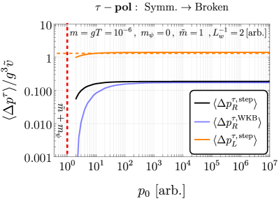
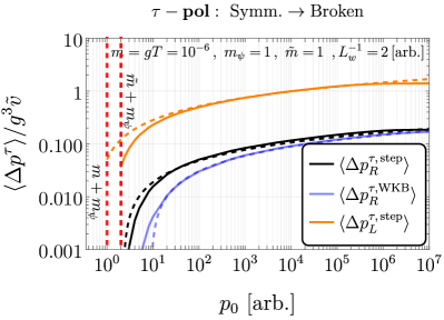
Figure 7: Symmetric $\to$ Broken. We present qualitatively the same plot as in fig. 3 (left panel), this time disentangling all the contributions, and highlighting the effect of a hierarchy $m\ll m_{\psi}$ for $\tau$ emission. Top Left: Averaged momentum exchange for $\tau$ polarisation contributions. The curves quickly saturate to their constant asymptotic values and the dominant contribution is $L-$mover emission in the step wall regime. Thick lines are numerics and the dashed line is the analytical expression in eq. 211. Top Right: Same as previous, but for $m/m_{\psi}\ll 1$. We see the transient inter-relativistic regime scaling as $\log(p_{0})$, well described by the $m=0$ analytical formulae (dashed lines) found in section E.4. The regime ends around $p^{0}\sim\tilde{m}m_{\psi}/m$. Bottom: $\lambda$ polarisation contributions. The result is quite insensitive to the symmetric side $\lambda$ mass $m_{h,s}(T)$ as long as it is $\lesssim\tilde{m}$. We plot for $m_{\psi}=1\ {\rm[arb.]}$, but varying it does not change much either; unlike for $\tau$, there is no intermediate regime. Dashed lines are analytical formulae in eqs. 219 and 220.

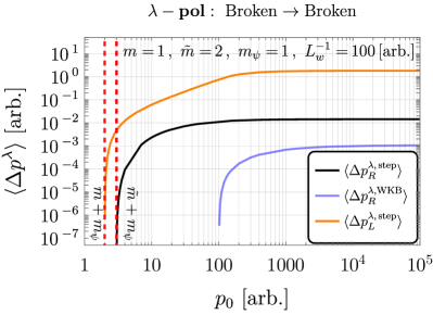
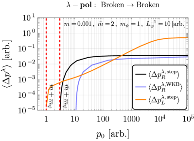
Figure 8: Broken $\to$ Broken. Left: Averaged momentum exchange for $\lambda$ polarisation emission for relatively thin wall. The inter-relativistic regime of scaling with $p^{0}$ lasts till $p^{0}\sim L_{w}^{-1}$. Taking $\Delta m\ll 1$ does not qualitatively change anything expect for suppressing all values. Notice $m\lesssim\tilde{m}$. Right: Similar to previous, but in the case $m\ll\tilde{m}$. Here we see that the inter-relativistic regime is distorted at low $p^{0}$ and also extended up to $p_{0}\sim L_{w}^{-1}m_{\psi}/m$.

We now report and comment on our results for the average NLO momentum transfer $\langle{\Delta p}\rangle$ due to transition radiation from a $\psi$ particle travelling across the wall and thereby compute the total pressure on the bubble wall. We show a break down of figs. 2 and 3 into all their contributions, as well as provide some analytical formulae. A comprehensive comparison (via numerical integration - see appendix E for some analytical evaluation of phase space integrals) of all the different parts in section 4.2 is shown in figs. 7 and 8, as a function of the energy of the incoming emitter particle, $\psi$. In the asymptotic $p_{0}\rightarrow\infty$ limit all contributions are constant. Their relative importance is displayed in fig. 9. We now discuss the two cases of interest $v=0$ and $v\neq 0$ separately.

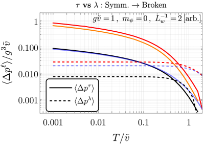
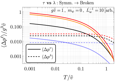
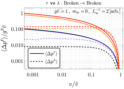
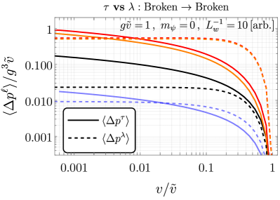
Figure 9: Here is presented the same plot as in fig. 2, but this time disentangling all the contributions. Solid lines refer to $\tau$ polarisation, while dashed to $\lambda$. Red lines are the total sum, for each polarisation. Top: Symmetric $\to$ Broken. It is shown two cases with different wall width and it is worth noticing that while the total contribution for $\tau$ and $\lambda$ does not change appreciably, the single contributions do, like $R$ step wall versus WKB. Bottom: Broken $\to$ Broken. Here it happens the same as in the top panels, but, since in this case $L$ step contribution from $\lambda$ polarisation has to be taken into account, we see that, depending on the value of $L_{w}$ and the hierarchy between the different vevs, can be the most relevant contribution.

Symmetric to broken case ($v=0$).

We observe in fig. 7 that when the emitting particle is $m_{\psi}\lesssim m$ the contribution from $\tau$ saturates quickly to the constant $p_{0}\to\infty$ value (top left in fig. 7), but if there is a hierarchy $m\ll m_{\psi}$, we observe an inter-relativistic regime of logarithmic dependence on $p_{0}$ up until $p_{0}\sim\tilde{m}m_{\psi}/m$. This can be traced to a collinear log divergence of phase space integration in the limit $m=0$ & $p_{0}\rightarrow\infty$ as explained in appendix E. This behaviour is not present in contributions from $\lambda$ polarisation emission, which are insensitive to $m_{\psi}$ for relativistic $p^{0}$, even when the symmetric side mass is set to zero $m_{h,s}=0$.

In the asymptotic $p^{0}\rightarrow\infty$ limit $\tau$ contributions depend significantly only on the ratio $m/\tilde{m}$, which can be translated to $T/\tilde{v}$. While individual $\lambda$ contributions depend also on $L_{w}^{-1}$ their sum is constant. The total momentum transfer (summing over all contributions) can be fitted by the following expression

$$\lim_{p_{0}\to\infty}\langle{{\Delta p}^{\rm total}}\rangle\simeq g^{3}\tilde{v}\left[0.135\log\left(\frac{\tilde{v}}{T}+2.26\right)-0.085-0.2\frac{\log\left(\frac{\tilde{v}}{T}+2.26\right)}{\tilde{v}/T}+\frac{0.19}{\tilde{v}/T}\right]\,.$$ (146)

We recall that to obtain this expression we cut the phase space integrals in the IR at energies $\sim gT$. The expression in eq. 146 becomes valid for the energies of initial particle $p_{0}\gtrsim\frac{\tilde{v}}{T}\times m_{\psi}$, which in the case of massless emitter $m_{\psi}\to 0$ becomes $p_{0}\gtrsim\tilde{v}$. The contribution of the longitudinal modes is sub-leading except perhaps for mild super-cooling $\tilde{v}/T\sim$few, and is equal approximately to

$$\lim_{p_{0}\to\infty}\langle{{\Delta p}^{\lambda}}\rangle\sim g^{3}\tilde{v}\times c_{\lambda}(L_{w},T,\tilde{m},m_{\psi}),~{}~{}~{}c_{\lambda}\in[0.02,0.03].$$ (147)

An analytical form for the function $c_{\lambda}$ is given in eq. 221.

So far we were calculating the momentum transfer from individual collisions. In order to find the pressure acting on the bubble wall we need to perform the integration over the flux of incoming particles. This can be easily done in the thermal case since we know the distributions

$${\cal P}=\int\frac{d^{3}p}{(2\pi)^{3}}f_{\psi}(T,\gamma_{w})\times\frac{p^{z}}{p_{0}}\langle{\Delta p}\rangle.$$ (148)

If the average momentum transfer is a constant the integration is simple and we find, since in the ultra-relativistic case $p^{z}/p_{0}\to 1$,

$${\cal P}=n_{\psi}(T,\gamma_{w})\langle{\Delta p}\rangle=\gamma_{w}n_{\psi}(T)\langle{\Delta p}\rangle,$$ (149)

where $n_{\psi}$ is the density of emitters $\psi$ defined in the plasma frame. Then, for the symmetric to broken transition we obtain the following expression for the pressure:

$$\lim_{\gamma_{w}\to\infty}{\cal P}_{\rm th.}\simeq \;\frac{\zeta(3)\gamma_{w}T^{3}}{\pi^{2}}\times$$ (150)

$$g^{3}\tilde{v}\left[0.135\log\left(\frac{\tilde{v}}{T}+2.26\right)-0.085-0.2\frac{\log\left(\frac{\tilde{v}}{T}+2.26\right)}{\tilde{v}/T}+\frac{0.19}{\tilde{v}/T}\right]\ ,$$

where the $\rm th.$ stands for thermal.

Broken to broken case ($v\neq 0$).

In fig. 8 we show the evolution of $\langle{\Delta p}\rangle(p_{0})$ for a broken to broken transition. We focus only on $\lambda$ contributions since the ones from $\tau$ are essentially the same as in fig. 7 with suitable re-interpretation of what $m,\tilde{m}$ mean (see section 4.2). Again the curves eventually saturate to a constant value but we highlight the strongly $L_{w}-$dependent novel contribution from $L-$mover emission, which easily comes to dominate in the thin wall regime. As in fig. 3, we highlight that in the left panel we can clearly distinguish the inter-relativistic region where this last contribution develops a linear growth in $p_{0}$. In fig. 9 we see the dependence of the saturation value of the averaged exchanged momentum (in the limit $p_{0}\to\infty)$ on the ratio between vevs (lower panels).

Broken to broken transitions were recently studied at leading order by [68] and it was found that reflection of the longitudinal vectors is efficient for the energies below $L_{w}^{-1}$ (inverse width of the wall). This in its turn lead to the pressure scaling as $\gamma_{w}^{2}$, as long as $p_{0}<L_{w}^{-1}$. We find that a reminiscent effect happens at NLO level, the main difference is that the momentum of the vector is not fixed by the speed of the bubble expansion and is always integrated over all possible values. We find that the momentum transfer is dominated by left-mover modes and for the values of the energies of incoming particle $p_{0}<L_{w}^{-1}{\rm Max}[1,m_{\psi}/m]$ it is proportional to $\propto p_{0}$

$$\lim_{p_{0}<L^{-1}_{w}{\rm Max}[1,m_{\psi}/m]}\langle{{\Delta p}_{v\neq 0}}\rangle\sim 10^{-2}\times g^{2}\frac{(v^{2}-\tilde{v}^{2})^{2}}{(v^{2}+\tilde{v}^{2})^{2}}\times\frac{p_{0}}{{\rm Max}[1,m_{\psi}/m]}\ .$$ (151)

In the case of large hierarchy $0<m\ll m_{\psi}$, not only is the saturation point delayed, but a further slight distortion occurs at low $p^{0}$, as shown in fig. 8. Once the energy of the initial particle becomes larger than $\sim L_{w}^{-1}{\rm Max}[1,m_{\psi}/m]$, we have

$$\lim_{p_{0}\to\infty,L\to 0}\langle{{\Delta p}_{v\neq 0}}\rangle\simeq 0.05g^{2}\frac{(v^{2}-\tilde{v}^{2})^{2}}{(v^{2}+\tilde{v}^{2})^{2}}L^{-1}_{w}.$$ (152)

Momentum transfer stops growing and reaches the saturation value. Note that the maximal value of this pressure is controlled by $L_{w}^{-1}$ and not by the mass of the vector $g\tilde{v}$. This is related to the fact that at high energies Goldstone Boson equivalence theorem relates the longitudinal vectors to the Goldstone bosons, and the strength of their interaction with the bubble wall (Higgs field) is controlled by the mass of the Higgs (wall width). Consequently, in the case of broken to broken transition, there is an additional contribution to the pressure which scales as

$$\lim_{\gamma_{w}\to\infty}{\cal P}^{\lambda}_{v\neq 0}\sim 0.05\frac{\zeta(3)\gamma_{w}T^{3}}{\pi^{2}}\times g^{2}\frac{(v^{2}-\tilde{v}^{2})^{2}}{(v^{2}+\tilde{v}^{2})^{2}}\times L_{w}^{-1}.$$ (153)

with an intermediate regime scaling as ${\cal P}^{\lambda}\propto\gamma_{w}^{2}$ for the values of boost factor $\gamma_{w}<(L_{w}T)^{-1}$.

5 Summary

We conclude by summarising the main results of our work. We analyzed in details the phenomena of transition radiation in the presence of domain walls. We quantised from first principles scalar and vector theories on a translation-violating background and identified the correct asymptotic states. We split emission into soft and UV regimes and used a step wall and WKB approximation respectively to compute the desired matrix elements for transition radiation. Quantisation of vector field theories was naturally performed via the introduction of new degrees of freedom which do not coincide with the traditional transverse and longitudinal polarisation but are a convenient admixture. In this way we have resolved some puzzles regarding the inclusion of longitudinal polarisations in the calculation of transition radiation.

We applied these results to calculate the pressure experienced by the bubble wall during the ultra-relativistic expansion. For the phase transitions with spontaneous breaking of the gauge symmetries in the regime of strong supercooling we find the pressure which scales as

$${\cal P}\propto\gamma_{w}g^{3}\tilde{v}T^{3}\log\frac{\tilde{v}}{T},~{}~{}~{}~{}\text{for}\quad\tilde{v}/T\gg 1,$$ (154)

and is dominated by the emission back out of the wall of transverse-like polarisations with momenta $k^{z}\in(0,\Delta m)$. This result qualitatively agrees with the previous literature on the subject. For moderate ratio $\tilde{v}/T\sim$ few we find that the contribution from the longitudinal-like polarisations can lead to significant corrections. We provide an updated fitted formula for the total pressure in section 4.3.

We also analyzed the pressure in the case of transition between two vacua with broken gauge symmetry. Interestingly we find in this case the contribution from the longitudinal-like polarisation can esily become dominant for thin walls, with the asymptotic value controlled by the inverse wall width ${\cal P}^{\rm max}\propto\gamma_{w}g^{2}T^{3}L_{w}^{-1}$. Moreover, we find a transient intermediate regime of ${\cal P}\propto\gamma_{w}^{2}$ scaling for $p_{0}\lesssim L_{w}^{-1}$.

Our results make an advance in understanding the balance between bubble acceleration and friction which plays a crucial role in determining most phenomenological consequences of FOPTs as well as their detection prospect at upcoming gravitational wave detectors.

Future outlook:

The work can be improved and generalised in several ways. An important remaining question is the inclusion of finite temperature effects in a robust first principles fashion (see for example the discussion in section 4.2). It is relatively easy, though cumbersome, to allow also for the emitting particle to feel the wall $m_{\psi}\rightarrow m_{\psi}(z)$. Though in the $\gamma_{w}\rightarrow\infty$ limit, any dependence on $m_{\psi}(z)$ should drop out, we saw how $m_{\psi}$ can distort the intermediate shape of $\mathcal{P}^{\rm NLO}(\gamma_{w})$ and ultimately finding the equilibrium velocity $v_{w}$ will require a full knowledge of this curve. Similarly one could rigorously quantise fermionic fields that change mass across the wall.

A possibly important direction is the analysis of multiple vector emissions, particularly in regimes with large logs, possible IR enhancements and back-reaction effects coming from the overdensity of soft vector bosons around the wall (see discussion in [66]). Furhtermore it would be interesting to compare our wall-shape-independent results with a full numerical calculation using a specific smooth wall ansatz (for example $tanh$). Finally, with some tweaks our expressions can be used to analyse pressure in qualitatively different types of FOPTs, such as spontaneous breaking of global symmetries, or even symmetry restoring transitions.

While our interest here was in friction, we emphasise that our set up is useful for rigorously computing any process / Feynman diagram in the presence of background walls which are not treated as a perturbation. Just as an example, one can easily re-purpose our expressions to compute the number of particles of a given species produced from collisions between an expanding bubble and surrounding particles . The spontaneous breaking of Lorentz/translational symmetry in the early universe results in a rich phenomenology which is only starting to be explored systematically.

Appendix A Wavepackets and asymptotic states

No wall:

Let us recall a few things in the usual manifestly translation-invariant case (no wall background). For clarity we will first focus on $1+1$ dimensions. For a scalar field theory, the field operator $\psi(t,z)$ is interpreted as creating a particle at position $z$ at time $t=0$. The position space wavefunction of a state is thus given by its inner product with $\langle 0|\psi$. The wavefunction of a single particle eigenstate of momentum $|k\rangle=\sqrt{2k^{0}}a_{k}^{\dagger}|0\rangle$ is, as expected,

$$\langle 0|\psi(t,z)|k\rangle =e^{-ik_{\mu}x^{\mu}}\ .$$ (155)

To derive formulae for observables such as scattering cross sections or emission probabilities involving realistic particles we have to crucially go through appropriately defined wavepackets that describe those asymptotic states, taking a limit of sharp momentum only at the end. A wavepacket state describing a particle with momentum peaked around $p$ and localised in space is given by

$$|\Psi_{p}\rangle\equiv\int_{-\infty}^{\infty}{dk^{z}\over(2\pi)\sqrt{2k^{0}}}f_{p}(k^{z})|k\rangle\ ,\qquad\langle\Psi_{p}|\Psi_{p}\rangle=\int{dk^{z}\over(2\pi)}|f_{p}(k^{z})|^{2}=1\ .$$ (156)

where $f_{p}(k^{z})$ is like a sharp Gaussian in $k^{z}$ peaked at $p^{z}$. Note there is no spacetime dependence in this expression (we are always in the Heisenberg picture). The limit to recover a momentum eigenmode is $f_{p}(k^{z})\longrightarrow(2\pi)^{3}\sqrt{2k^{0}}\delta(p^{z}-k^{z})$. However, the more appropriate limit used in the derivation of physical rates makes use of the normalisation condition above

$$|f_{p}(k^{z})|^{2}\longrightarrow(2\pi)\delta(p^{z}-k^{z})\ ,\quad\text{(peaked momentum limit)}\ .$$ (157)

To see the localisation we can look at the wavefunction of the wavepacket state:

$$\langle 0|\psi(t,z)|\Psi_{p}\rangle =\int_{-\infty}^{\infty}{dk^{z}\over(2\pi)\sqrt{2k^{0}}}f_{p}(k^{z})e^{-ik_{\mu}x^{\mu}}\ .$$ (158)

At $t=0$ this is a an oscillating function of $z$ (with wavelength controlled by $p$) with a Gaussian envelope so that it is indeed localised at $z=0$. As a function of time, the wavepacket moves in the direction of sign$(p)$. Because each mode has a slightly different dispersion relation, the spatial width of the wavepacket tends to widen in time (dispersion) but this can be counteracted by making $f_{p}(k)$ a sharper Gaussian, taking an appropriate order of limits.

A.1 Asymptotic states in the wall background

In the presence of the wall we should still define asymptotic particle states as appropriate wavepackets to compute formulae for physical rates. A slight complication comes from the fact that the one particle states $|k_{L,R}\rangle$ we quantise are not eigenstates of momentum. Moreover, in general the same state describes different types of particles in different regions of space. Defining the asymptotic state carefully will get rid of any ambiguity.

We now consider an operator that feels the wall $\phi(t,\vec{x})$ expanded in left and right mover modes as in section 2.2. As before, the action of this on the vacuum should be thought of as creating a particle localised at $x^{\mu}=0$. Contracting a state with $\langle 0|\phi$ still gives the wavefunction understood in the usual sense. In fact

$$\langle 0|\phi(t,\vec{x})|k_{I}\rangle =e^{-ik_{n}x^{n}}\chi_{I,k}(z)\ ,$$ (159)

with $I={R,L}$. To gain physical intuition of the one particle states $|k_{I}\rangle$, consider constructing wavepackets by superimposing exclusively right (left) movers:

$$|\Phi^{\rm in}_{I,p}\rangle \equiv\int_{0,\>\Delta m}^{\infty}{dk^{z}\over(2\pi)\sqrt{2k^{0}}}f_{p}(k^{z})|k_{I}\rangle\ ,$$ (160)

where again we focus on $1+1$ dimensions and where the lower limit is $0$ $(\Delta m)$ for R (L) movers respectively. The ‘in’ labels will become clear shortly. Their wavefunctions are respectively

$$\langle 0|\phi(t,z)|\Phi^{\rm in}_{I,p}\rangle \equiv\int_{0,\>\Delta m}^{\infty}{dk^{z}\over(2\pi)\sqrt{2k^{0}}}f_{p}(k^{z})e^{-ik^{0}t}\chi_{I,k}(z)\ .$$ (161)

Ignoring the slight dispersion mentioned at the end of the previous subsection, the time evolution of eq. 161 for $I=R(L)$ describes an isolated localised wavepacket travelling in towards the wall from $z<0$ $(z>0)$ when $t<0$. This wavemode scatters off the wall and for $t>0$ splits into reflected and transmitted wavemodes travelling in opposite directions. Thus, $|\phi^{\rm in}_{R,p}\rangle$ ($|\phi^{\rm in}_{R,p}\rangle$) is a good asymptotic state for an incoming particle with positive (negative) $z-$momentum. It cannot however be used as an asymptotic state for any single outgoing asymptotic particle since at late times it describes a superposition.

So what about single localised outgoing particles? Clearly, when the wave equation is reduced to Schrodinger-like form with a real potential, these can be obtained by complex conjugation of the spacial part of the wavefunction. In other words we require states $|\Phi^{\rm out}_{I,p}\rangle$ such that

$$\begin{split}&\langle 0|\phi(t,z)|\Phi^{\rm out}_{I,p}\rangle\equiv\int_{\Delta m,\>0}^{\infty}{dk^{z}\over(2\pi)\sqrt{2k^{0}}}f_{p}(k^{z})e^{-ik^{0}t}\zeta_{I,k}(z)\\ &\text{with}\quad\zeta_{R,L}(z)=\chi_{L,R}^{*}(z)\end{split}$$ (162)

In time, these corresponds to two waves coming from opposite sides of the wall, hitting the wall around $t\approx 0$ and interfering in just the right way so that at late time there is only one wavemode travelling towards $z\rightarrow-\infty$ or $z\rightarrow\infty$ respectively. Notice the swap in labels. We adopt the convention that the right-mover $R$ (left-mover $L$) label always denotes a particle of positive (negative) $z-$momentum. It is an easy exercise to write the $\zeta_{R,L}$ in terms of a linear composition of the complete basis $\chi_{R,L}$ as explicitly done in eqs. 22 and 23. The appropriate wavepacket for an outgoing state is thus

$$|\Phi^{\rm out}_{I,p}\rangle \equiv\int_{\Delta m,\>0}^{\infty}{dk^{z}\over(2\pi)\sqrt{2k^{0}}}f_{p}(k^{z})|k^{\rm out}_{I}\rangle\ ,$$ (163)

where $|k^{\rm out}_{I}\rangle$ are the one-particle states with wavefunctions $\zeta_{I,k}(z)$ and are related to the $|k_{I}\rangle$ by

$$|k^{\rm out}_{L}\rangle =r_{R,k}^{*}|k_{R}\rangle+t_{R,k}^{*}\sqrt{\tilde{k}^{z}/k^{z}}\;|k_{L}\rangle\;\Theta(k^{z}-\Delta m)\ ,$$ (164)

$$|k^{\rm out}_{R}\rangle =t_{L,k}^{*}\sqrt{k^{z}/\tilde{k}^{z}}\;|k_{R}\rangle+r_{L,k}^{*}|k_{L}\rangle\ ,$$ (165)

where the reflection and transmission coefficients were defined in general for scalar d.o.f. in section 2.1, and given explicit form in the case of a step wall for fundamental scalars also in section 2.1 and for different vector polarisations in section 3.3.

Reflection and transmission probabilites:

As a consistency check we can compute reflection and transmission probabilities in this language. Focusing on the identity part of the S matrix $S=1+\cancel{i\mathcal{T}}$, the amplitude for a particle incoming from $z<0$ to reflect and transmit should be respectively

$$\langle\phi^{\rm out}_{L,p}|\phi^{\rm in}_{R,p}\rangle =\int_{0}^{\infty}{dk\over 2\pi}|f_{p}(k)|^{2}\;r_{R,k}\quad\rightarrow\quad r_{R,p}$$ (166)

$$\langle\phi^{\rm out}_{R,p}|\phi^{\rm in}_{R,p}\rangle =\int_{\Delta m}^{\infty}{dk\over 2\pi}|f_{p}(k)|^{2}\;t_{L,k}\sqrt{\tilde{k}^{z}/k^{z}}\quad\rightarrow\begin{cases}t_{L,p}\sqrt{p/\tilde{p}}\ ,&p>\Delta m\\ 0\ ,&p<\Delta m\end{cases}$$ (167)

where the arrow denotes taking the peaked momentum limit eq. 157 in the end. So the relative probability for a peaked-around-$p$ incoming mode to reflect / transmit into a peaked-around-$p$ outgoing mode is what one could have already guessed

$${\rm Reflection\ probability}=|\langle\phi^{\rm out}_{L,p}|\phi^{\rm in}_{R,p}\rangle|^{2} \rightarrow|r_{p}|^{2}$$ (168)

$${\rm Transmission\ probability}=|\langle\phi^{\rm out}_{R,p}|\phi^{\rm in}_{R,p}\rangle|^{2} \rightarrow\begin{cases}|t_{L,p}|^{2}p/\tilde{p}\ ,&p>\Delta m\\ 0\ ,&p<\Delta m\end{cases}$$ (169)

A.2 Phase space derivation from wavepackets

In this section we will obtain formulae for the averaged momentum exchanged by transition radiation processes in the background of the wall, deriving eq. 33 in the main text. Treating the incoming particle as a wavepacket as in eq. 156, we find the amplitude squared for splitting into $\ell$ particles, which may or may not feel the wall. These outgoing states are late-time eigenstates of momentum, obtained as limits of their their own wave-packet forms. We have

$$|\langle k_{1}^{\rm out}\dots k_{\ell}^{\rm out}|\Phi_{p}\rangle|^{2} =\int{d^{3}p_{1}d^{3}p_{2}\over\sqrt{4p^{0}_{1}p_{2}^{0}}}f_{p}(p_{1})f_{p}^{*}(p_{2})\delta^{(3)}\left(p_{1}-\underset{{i=1}}{\overset{\ell}{\Sigma}}k_{i}\right)\delta^{(3)}\left(p_{2}-\underset{{j=1}}{\overset{\ell}{\Sigma}}k_{i}\right)|\mathcal{M}^{(3)}_{1\rightarrow\ell}|^{2}$$

$$=\int{d^{3}p_{1}dp^{z}_{2}\over\sqrt{4p^{0}_{1}p_{2}^{0}}}f_{p}(p_{1})f_{p}^{*}(p_{2})\delta^{(3)}\left(p_{1}-\underset{{i=1}}{\overset{\ell}{\Sigma}}k_{i}\right){p^{0}_{1}\over|p^{z}_{1}|}\delta\left(p_{1}^{z}-p_{2}^{z}\right)|\mathcal{M}^{(3)}_{1\rightarrow\ell}|^{2}$$

$$=\int{d^{3}p_{1}\over 2|p^{z}_{1}|}|f_{p}(p_{1})|^{2}\delta^{(3)}\left(p_{1}-\underset{{i=1}}{\overset{\ell}{\Sigma}}k_{i}\right)|\mathcal{M}^{(3)}_{1\rightarrow\ell}|^{2}$$

$$\longrightarrow\frac{(2\pi)^{3}}{2|p^{z}|}\delta^{(3)}\left(p-\underset{{i=1}}{\overset{\ell}{\Sigma}}k_{i}\right)|\mathcal{M}^{(3)}_{1\rightarrow\ell}|^{2}\ ,$$ (170)

where the temporary label $(3)$ on $\mathcal{M}$ emphasises only three of $4-$momentum are conserved. in the the last step we take the peaked momentum limit of eq. 157. For the particular case of a $1\rightarrow 2$ process as discussed in this work, we have

$$\langle\Delta p^{z}_{I=R,L}\rangle\equiv\int\mathcal{P}_{p\rightarrow qk_{I}^{\rm out}}\Delta p^{z}_{I} =\int\frac{d^{3}k}{(2\pi)^{3}2k^{0}}\int\frac{d^{3}q}{(2\pi)^{3}2q^{0}}|\langle q\>k_{I}^{\rm out}|\Phi_{p}\rangle|^{2}\Delta p^{z}_{I}$$

$$=\int{d^{3}kd^{3}q\over(2\pi)^{3}8p^{z}k^{0}q^{0}}\delta^{(3)}\left(p-k-q\right)|\mathcal{M}_{I}^{(3)}|^{2}\Delta p^{z}_{I}$$

$$=\int{d^{3}k\over(2\pi)^{3}8p^{z}k^{0}|q^{z}_{k}|}\left[|\mathcal{M}_{I}^{(3)}|^{2}\Delta p^{z}_{I}\right]_{q^{z}=\pm q^{z}_{k}}$$ (171)

where in going to the last line we have used

$$\begin{split}\delta\left(p^{0}-k^{0}-q^{0}\right)={q^{0}\over|q^{z}_{k}|}\left[\delta(q^{z}-q^{z}_{k})+\delta(q^{z}+q^{z}_{k})\right]\\ \text{with}\quad q^{z}_{k}=\sqrt{(p^{0}-k^{0})^{2}-k_{\perp}^{2}-m_{q}^{2}}\end{split}$$ (172)

Thus, in principle one should sum contributions from both signs of $q^{z}$ to obtain the full integrated rate. In practice, the $q^{z}<0$ branch will be highly sub-leading at large energies.

Comparison with decay formula:

One might wonder how to recover the familiar decay formula in the limit of no wall. The latter can be derived in terms of the full $4-$momentum conserving matrix element $\mathcal{M}^{(4)}$ as

$$|\langle k_{1}\dots k_{\ell}|p\rangle|^{2} =\int{d^{3}p_{1}d^{3}p_{2}(2\pi)^{2}\over\sqrt{4p^{0}_{1}p_{2}^{0}}}f_{p}(p_{1})f_{p}^{*}(p_{2})\delta^{(4)}\left(p_{1}-\underset{{i=1}}{\overset{\ell}{\Sigma}}k_{i}\right)\delta^{(4)}\left(p_{2}-p_{2}\right)|\mathcal{M}^{(4)}_{1\rightarrow\ell}|^{2}$$

$$=\int{d^{3}p_{1}(2\pi)^{2}\over 2p_{1}^{0}}|f_{p}(p_{1})|^{2}\delta^{(4)}\left(p_{1}-\underset{{i=1}}{\overset{\ell}{\Sigma}}k_{i}\right)\underbrace{\delta\left(0\right)}_{T/2\pi}|\mathcal{M}^{(4)}_{1\rightarrow\ell}|^{2}$$

$$\longrightarrow\frac{(2\pi)^{4}}{2p_{0}}\mathbb{T}\;\delta^{(4)}\left(p-\underset{{i=1}}{\overset{\ell}{\Sigma}}k_{i}\right)|\mathcal{M}^{(4)}_{1\rightarrow\ell}|^{2}\ ,$$ (173)

where $\mathbb{T}$ is total time (one can only define a decay probability per unit time). We can see how eq. 170 reduces to this result. In the absence of the wall the matrix element gives

$$|\mathcal{M}^{(3)}_{1\rightarrow\ell}|^{2} =2\pi\>\mathbb{L}^{z}\delta\left(p^{z}-\underset{{i=1}}{\overset{\ell}{\Sigma}}\right)|\mathcal{M}^{(4)}_{1\rightarrow\ell}|^{2}$$ (174)

where $\mathbb{L}^{z}$ is the distance traversed in the $z$ direction. Finally, using that $\mathbb{L}^{z}=\mathbb{T}\;p^{z}/p^{0}$, eq. 170 reduces to eq. 173.

Appendix B Current conservation in the presence of the wall

In the main text we have discussed the modifications of the Ward identities in the presence of the wall and that in general the conserved current coupled to the total derivative must give zero matrix element,

$$J^{\mu}\partial_{\mu}f~{}~{}~{}\Rightarrow\langle final|\>\mathcal{S}_{f}\>|initial\rangle=0\ .$$ (175)

Let us discuss the effects of various choices of the gauge transformation function $f$. For example let us consider $f=\chi_{1,2}^{\tau}(z)$, where $\chi_{1,2}^{\tau}$ are the wave functions for the $\tau$ polarisations (see section 3.2). Then the matrix element will be equal to

$$J^{\mu}\propto(p+q)^{\mu}~{}~{}~{}~{}\Rightarrow~{}~{}~{} \mathcal{M}=\frac{(p+q)_{\mu}k^{\mu}}{\Delta p}+r^{\tau}_{k}\frac{(p+q)_{\mu}k^{\mu}_{r}}{\Delta p_{r}}-t^{\tau}_{k}\frac{(p+q)_{\mu}\tilde{k}^{\mu}}{\Delta\tilde{p}}\ ,$$ (176)

$$k_{r}^{\mu}\equiv(k^{m},-k^{z}),~{}~{}~{}\tilde{k}^{\mu}\equiv(k^{m},\tilde{k}^{z})\ .$$

We can simplify the amplitude using the following identities:

$$(p+q)_{\mu}k^{\mu} =(p+q)_{m}k^{m}-(p+q)_{z}k^{z}$$

$$\overset{k_{m}=(p-q)_{m}}{=}(p+q)_{m}(p-k)^{m}-(p+q)_{z}k^{z}$$

$$=p_{z}^{2}+m_{\psi}^{2}-q_{z}^{2}-\tilde{m}_{\psi}^{2}-(p+q)_{z}k^{z}$$

$$\overset{m_{\psi}^{2}=\tilde{m}_{\psi}^{2}}{=}(p+q)_{z}(p-q-k)^{z}=(p+q)_{z}\Delta p\ .$$ (177)

Performing similar manipulations for all of the terms we get:

$$\mathcal{M}=(p+q)_{z}(1+r^{\tau}_{k}-t^{\tau}_{k})=0\ ,$$ (178)

where we used the fact that $1+r^{\tau}_{k}-t^{\tau}_{k}=0$ for $\tau$ polarisations, as expected. Similarly we can choose $f=\alpha(z)$, of the $\lambda$. Then from the eq. (110) we can get

$$\alpha|_{z<0} =\frac{ik^{z}}{gvE}\left(e^{ik^{z}z}-r^{\lambda}_{k}e^{-ik^{z}z}\right)\ ,$$

$$\alpha|_{z>0} =it^{\lambda}_{k}\times\frac{\tilde{k}^{z}}{gE\tilde{v}}e^{i\tilde{k}^{z}z}\ ,$$ (179)

where we have used that $\alpha=\frac{1}{gv^{2}E}\partial_{z}(v\lambda)\to\frac{1}{gEv}\partial_{z}\lambda$ outside of the wall. Using the expression for reflection and transmission coefficients from eq. 112

$$r^{\lambda}_{k}=\frac{\tilde{v}^{2}k^{z}-v^{2}\tilde{k}^{z}}{\tilde{v}^{2}k^{z}+v^{2}\tilde{k}^{z}}\ ,\qquad t^{\lambda}_{k}=\frac{2k^{z}v\tilde{v}}{\tilde{v}^{2}k^{z}+v^{2}\tilde{k}^{z}}\ ,$$ (180)

we can compute the amplitude for the processes $J^{\mu}\to\chi_{\lambda}^{\mu}$ corresponding to the interaction $J_{\mu}\chi_{\lambda}^{\mu}$. The computation goes as follows

$$\mathcal{M} = \frac{k^{z}}{gEv}\frac{(p+q)_{\mu}k^{\mu}}{\Delta p}-\frac{k^{z}}{Egv_{1}}r^{\lambda}_{k}\frac{(p+q)_{\mu}k^{\mu}_{r}}{\Delta p_{r}}-\frac{\tilde{k}^{z}}{gE\tilde{v}}t^{\lambda}_{k}\frac{(p+q)_{\mu}\tilde{k}^{\mu}}{\Delta\tilde{p}}$$ (181)

$$= \frac{(p+q)_{z}}{E}\underbrace{\bigg{(}\frac{k^{z}}{gv}-\frac{k^{z}}{gv}r^{\lambda}_{k}-\frac{\tilde{k}^{z}}{g\tilde{v}}t^{\lambda}_{k}\bigg{)}}_{=0}=0\ ,$$

the last expression in brackets is the matching condition for the $\lambda$ field (section 3.3.2) which must be satisfied. Note that terms cancelling each other in the brackets are growing in energy, which makes crucially important the calculation of exact values of reflection and transmission coefficients.

Appendix C WKB regime in the case of current non-conservation

In the main text we focus only on the transition radiation from the conserved current. How we can perform a similar calculation in the case when the current is not conserved? Let us consider the following example with scalar fields

$${\cal L} =-\frac{1}{4}F_{\mu\nu}F^{\mu\nu}+|D_{\mu}H|^{2}-V(|H|)+|D_{\mu}\phi|^{2}-m_{\psi}^{2}|\phi|^{2}+\left(\kappa\phi^{2}H+h.c.\right).$$

The charges under the gauged $U(1)$ symmetry are as follows: $Q_{U(1)}(H)=1,Q_{U(1)}(\phi)=-1/2$. In the section 3.5, in order to perform the WKB calculation and get rid off interactions which can potentially lead to the divergences we have used the current conservation equations to modify the expression for the matrix elements. In the case of the system in appendix C the divergence of the current becomes equal to:

$$\partial_{\mu}J_{\phi}^{\mu}=\sqrt{2}v(z)\left(\kappa^{*}\phi^{*2}-\kappa\phi^{2}\right)\ ,~{}~{}~{}J_{\phi}^{\mu}=i(\phi^{*}\partial^{\mu}\phi-\phi\partial^{\mu}\phi^{*})\ .$$ (183)

The interaction between the $\lambda$ polarisation and $J_{\phi}^{\mu}$ and can be written as follows:

$$gQ_{\phi}J_{\phi}^{\mu}A_{\mu}^{(\lambda)}\to Q_{\phi}\left[-\sqrt{2}\left(\kappa^{*}\phi^{*2}-\kappa\phi^{2}\right)\frac{1}{Ev(z)}\partial_{z}\left(v(z)\lambda(z)\right)-\frac{g^{2}v(z)}{E}\lambda(z)J_{z}\right]\ .$$ (184)

We can see that on top of the term $\lambda J_{z}$ present in the conserved current case, there is an additional interaction. However this interaction is not growing with energy, and in the limit $v(z)\to 0$, it is finite (see discussion in the appendix D), thus the calculation of the vector emission becomes straightforward.

Appendix D Properties of the potential for $\lambda$ field

In the main text we have shown that $\lambda$ field satisfies the following equation of motion eq. 81$-$(82)

$$\left(-E^{2}-\partial_{z}^{2}+U_{\lambda}(z)\right)\lambda=0\ ,$$

$$U_{\lambda}(z)=g^{2}v^{2}(z)+2\left(\partial_{z}v\over v\right)^{2}-{\partial_{z}^{2}v\over v}\ .$$ (185)

Let us investigate the properties of the function $U_{\lambda_{z}}$.

Broken$\to$ Broken

In this case

$$v_{z\to\pm\infty}\neq 0\ ,$$ (186)

and the potential has the limits :

$$U_{\lambda}(z)|_{z\to\pm\infty}=g^{2}v^{2}(z\to\pm\infty)\ ,$$ (187)

where we have used that $v^{\prime},v^{\prime\prime}\to 0$ outside of the wall. Physics wise this result is expected since $\lambda$ mode must have the mass of the vector $gv$ outside of the wall.

Symmetric$\to$Broken

Here we will assume

$$v(z\to-\infty)=0\ ,~{}~{}~{}v(z\to\infty)=\tilde{v}\neq 0\ .$$ (188)

On the broken side as expected

$$U_{\lambda}(z\to\infty)=g^{2}v^{2}(z\to\infty)=g^{2}\tilde{v}^{2}\ ,$$ (189)

the potential becomes equal to the mass square of the vector boson. To find its limit on the symmetric side we need to look at the equation defining $v(z)$:

$$\partial_{z}^{2}v(z)=V^{\prime}(v(z))\ ,$$ (190)

where the prime stands for a derivative with respect to $v(z)$. Integrating this equation we get

$${1\over 2}\;(\partial_{z}v(z))^{2}=V(v(z))-C\ ,$$ (191)

where $C=-(\partial_{z}v(z_{0}))^{2}+V(v(z_{0}))$ is a ‘constant of integration’. We can choose $z_{0}\to-\infty$, then using $v^{\prime},v\to 0$ we get $C=V(v(-\infty))=V(0)$, which need not to be zero. Now we look at the limits as $z\rightarrow-\infty$. At this point, using eqs. (190) and (191) we can write the various terms of the $U_{\lambda}$ function in terms of the potential $V$ and its derivatives $V^{\prime}$:

$${\partial_{z}^{2}v(z)\over v(z)} = {\partial_{z}^{2}v\over v}={V^{\prime}(v)\over v}\overset{v\to 0}{\longrightarrow}V^{\prime\prime}(0)\ ,$$

$$\left(\partial_{z}v(z)\over v(z)\right)^{2} = \left(\partial_{z}v\over v\right)^{2}=2{V(v)-V(0)\over v^{2}}\overset{v\to 0}{\longrightarrow}V^{\prime\prime}(0)\ .$$ (192)

In the limit $z\to-\infty,v\to 0$, however we know that the first derivative of the potential $V$ must be equal to zero at this point

$$\frac{\partial V}{\partial v}|_{v\to 0}=0\ ,$$ (193)

since there is a local minimum at $v=0$. Thus in the region $v\to 0$ we can write down:

$$V(v)|_{v\to 0} = \frac{V^{\prime\prime}(0)v^{2}}{2}+V(0)\Rightarrow$$

$$\frac{V^{\prime}(v))}{v}|_{v\to 0} = V^{\prime\prime}(0)\ ,~{}~{}~{}2{V(v)-V(0)\over v^{2}}=V^{\prime\prime}(0)\ .$$ (194)

Combining these results we can see that

$$\lim\limits_{z\to-\infty}U_{\lambda}(z)=V^{\prime\prime}(0)=m_{h,s}^{2}\ ,$$ (195)

where $m_{h,s}$ is the mass of the scalar on the symmetric side. We can see that as was discussed in the section 3.2 $U_{\lambda}$ has the correct properties for a potential of a d.o.f interpolating between the scalar field and $\lambda$ polarisation on different sides of the wall.

Appendix E Evaluation of phase space Integrals

In this appendix we provide some details regarding the evaluation of the phase space integrals, and how to derive analytical expressions. We will always be interested in the limit of large incoming energy $p^{0}\gg$ all masses. The type of integrals we deal with are all of the form

$$I(p^{0})=\int^{l_{1}(p^{0})}_{\rm const}dk\int^{l_{2}(p^{0},k)}_{\rm const^{\prime}}dk_{\perp}^{2}\;{\rm Int}(p^{0},k,k_{\perp}^{2})\ ,$$ (196)

where the dependence on couplings and masses $m_{i}$ is implicit. When $I(p^{0})$ admits an expansion around infinity, this can be obtained in principle straightforwardly as

$$I(p^{0})=\left.I(1/x)\right|_{x\rightarrow 0}+\left.{d\over dx}I(1/x)\right|_{x\rightarrow 0}\;{1\over p^{0}}+\;\dots$$ (197)

and one can sometimes take this ‘exact’ approach. However, such an expansion does not always exist , or if it does, its coefficients might in practice be difficult to evaluate. Moreover, in the presence of large mass hierarchies, the regime where eq. 197 is actually a good approximation can begin at arbitrary high energies . One can often successfully use a different expansion instead, which we call ‘collinear expansion’, of $p^{0},k^{z}\gg k_{\perp},m_{i}$ where $m_{i}$ stands for all masses. Keeping the leading term, this reduces integrands to the form

$${\rm Int}(p^{0},k,k_{\perp}^{2})={N(k,k_{\perp},m_{i})\over\left[(k^{IR}_{\perp,m})^{2}+k_{\perp}^{2}\right]^{2}}\qquad\text{for}\quad p^{0},k^{z}\gg k_{\perp},m_{i},$$ (198)

where

$$k_{\perp}^{2}\lesssim(k^{IR}_{\perp,m})^{2}\equiv{k_{z}^{2}m_{\psi}^{2}-k^{z}m^{2}p_{0}\over(p_{0})^{2}}+m^{2}>0\,.$$ (199)

The function $N$ depends on the contribution in question but we wish to highlight the factor in denominator. This form makes most manifest the properties of the phase space structure in particular for $\tau$ polarisation (and scalars), most importantly when $m$ (and possibly $m_{\psi}$) is very small. For a given $k^{z}$, the integrand is peaked for $k_{\perp}^{2}\lesssim(k^{IR}_{\perp,m})^{2}$. Notice the role of $k^{IR}_{\perp,m}$ - its presence regulates an otherwise logarithmically IR divergent integral. Indeed the momentum transfer diverges in the limit of $m,m_{\psi}\rightarrow 0$. It is easy to prove that $k^{IR}_{\perp,m}<k^{z}$ for small $m$, justifying the expansion. When $m/m_{\psi}$ is very small, clearly there are two relativistic regimes, the first given by

$$p^{0}\lesssim k^{z}m_{\psi}/m\,,$$ (200)

where $k^{z}$ should be taken in the dominant region. Typically $k^{z}\sim\tilde{m}$ for step function contributions and $\sim L_{w}^{-1}$ for WKB. Above this scale instead one reaches the true asymptotic behaviour where eq. 197 is valid.

E.1 Scalars

Scalar $R$-mover emission (WKB)

We begin with the most dominant contribution to scalar emission at the highest of energies $p^{0}\rightarrow\infty$. The amplitude is the simplest that one can encounter,

$$\mathcal{M}_{R}^{\rm wkb}=\left({y\over i\Delta p}+{\tilde{y}\over-i\Delta\tilde{p}}\right)\ ,$$ (201)

and

$$\langle\Delta p^{\rm wkb}_{R}\rangle =\int_{L^{-1}_{w}}^{k^{z}_{\rm max}}{\;dk^{z}}\int^{k_{\perp,cut}^{2}}_{0}{d{k_{\perp}^{2}}\over 2}\frac{|\mathcal{M}_{R}^{\rm wkb}|^{2}}{(2\pi)^{2}8p^{z}q^{z}k_{0}}\Delta p_{R}\ .$$ (202)

For $m\neq 0$, properly evaluating the expansion eq. 197 for this case is tricky . However the collinear expansion eq. 198 works extremely well, giving

$$\langle\Delta p^{\rm wkb}_{R}\rangle \approx{y^{2}\Delta m^{4}\over 32\pi^{2}}\int_{L^{-1}_{w}}^{k^{z}_{\rm max}}{\;dk^{z}}\int^{k_{\perp,cut}^{2}}_{0}dk_{\perp}^{2}{(k^{z}-p_{0})^{2}/(p_{0})^{4}\over\left[(k^{IR}_{\perp,m})^{2}+k_{\perp}^{2}\right]^{2}\left[(k^{IR}_{\perp,\tilde{m}})^{2}+k_{\perp}^{2}\right]}\ ,$$ (203)

where $k^{IR}_{\perp}$ is given by eq. 199. We see indeed that for large $p^{0}$ the integrand is relatively flat in $k^{z}$ while $k_{\perp}$ is strongly IR dominated as anticipated in the preamble above, justifying the expansion. The integrals can now be computed exactly and we obtain eq. 51. We can see clearly however that there is also an intermediate regime for small $m/m_{\psi}$ characterised by a plateau:

$$\langle\Delta p^{\rm wkb}_{R}\rangle \approx\begin{cases}{y^{2}\tilde{m}^{2}L_{w}\over 32\pi^{2}m_{\psi}^{2}}\ ,&L^{-1}\ll p^{0}\lesssim L^{-1}_{w}{m_{\psi}\over m}\\ \lx@cref{creftype~refnum}{eq:WKBScalars}\ ,&p^{0}\gtrsim L^{-1}_{w}{m_{\psi}\over m}\end{cases},$$ (204)

where we remind ourselves that there is no WKB contribution at all unless we can emit modes greater than the inverse wall length. The value of the plateau is easily obtained by setting $m=0$ at the start and computing the leading order in eq. 197. However, in this regime, we find the step function contributions are more important and we move on there now.

Scalar $R$ and $L$-mover emission (step wall)

The step wall case is an interesting theory exercise in its own right, since everything can be done exactly. For scalars the contributions are

$$\langle\Delta p^{\rm step}_{R}\rangle =\int_{\Delta m}^{L^{-1}_{w}}{\;dk^{z}}\int^{k_{\perp,\rm max}^{2}}_{0}{d{k_{\perp}^{2}}\over 2}\frac{|\mathcal{M}_{R}^{\rm step}|^{2}}{(2\pi)^{2}8p^{z}q^{z}k_{0}}\Delta p_{R}\ .$$ (205)

$$\langle\Delta p^{\rm step}_{L}\rangle =\int_{0}^{L^{-1}_{w}}{\;dk^{z}}\int^{k_{\perp,\rm max}^{2}}_{0}{d{k_{\perp}^{2}}\over 2}\frac{|\mathcal{M}_{L}^{\rm step}|^{2}}{(2\pi)^{2}8p^{z}q^{z}k_{0}}\Delta p_{L}\ .$$ (206)

where the matrix elements are given by eqs. 29 and 30. Evaluating these in the asymptotic limit we obtain

$$\langle\Delta p_{L}^{\rm step}\rangle \approx{y^{2}\tilde{m}\over 32\pi^{2}m_{\psi}^{2}}\begin{cases}4\ ,&p_{0}\lesssim\tilde{m}m_{\psi}/\sqrt{3}m\\ {4m_{\psi}^{2}\Delta m\over 3\tilde{m}m^{2}p_{0}^{2}}\left[m^{2}\left(\ln{m^{2}\over\tilde{m}^{2}}-1\right)+\tilde{m}^{2}\right]\ ,&p_{0}\gtrsim\tilde{m}m_{\psi}/\sqrt{3}m\end{cases}$$ (207)

$$\langle\Delta p_{R}^{\rm step}\rangle \approx{y^{2}\tilde{m}\over 32\pi^{2}m_{\psi}^{2}}\begin{cases}1-\tilde{m}L_{w}\ ,&p_{0}\lesssim m_{\psi}\tilde{m}/m\\ {m_{\psi}^{2}(L_{w}^{-1}-\Delta m)\over 4\tilde{m}m^{2}p_{0}^{2}}\left[\Delta m^{2}+2m^{2}\ln\left(m\over\tilde{m}\right)\right]\ ,&p_{0}\gtrsim m_{\psi}\tilde{m}/m\end{cases}$$ (208)

E.2 Vectors: $\tau$ emission

The three relevant amplitudes are repeated here again

$$\begin{split}\mathcal{M}^{\rm step}_{\tau,L}&=-ig\epsilon_{\tau_{2}}^{\mu}(p+q)_{\mu}\left(\frac{1}{\Delta p_{r}}+\frac{r_{\tau,k}}{\Delta p}+\frac{t_{\tau,k}}{-\Delta\tilde{p}_{r}}\right)\ ,\\ \mathcal{M}^{\rm step}_{\tau,R}&=-ig\sqrt{k^{z}\over\tilde{k}^{z}}\epsilon_{\tau_{2}}^{\mu}(p+q)_{\mu}\left[\frac{\tilde{k}^{z}}{k^{z}}\frac{t_{k}}{\Delta p}-\frac{1}{\Delta\tilde{p}}+\frac{r_{k}}{\Delta\tilde{p}_{r}}\right]\ ,\\ \mathcal{M}^{\rm wkb}_{\tau}&=-ig\epsilon_{\tau_{2}}^{\mu}(p+q)_{\mu}\left(\frac{1}{\Delta p_{r}}+\frac{1}{-\Delta\tilde{p}}\right)\ .\end{split}$$ (209)

For $\tau$ polarisation we can treat both types of transitions of interest at the same time by interpreting the $m,\tilde{m}$ correctly.

E.3 $m\neq 0$ asymptotic $p^{0}$ regime

We present now the dominant contribution $\mathcal{M}^{\rm step}_{\tau,L}$ in detail . The amplitude squared is

$$\left|\mathcal{M}^{\rm step}_{\tau,L}\right|^{2} =\frac{16g^{2}k_{z}^{2}k_{\perp}^{2}p_{0}^{2}}{(k_{z}^{2}+m^{2})(k_{z}^{2}-(p^{z}-q^{z})^{2})^{2}}\begin{cases}\frac{\Delta m^{2}}{\Delta m^{2}-k_{z}^{2}+(p^{z}-q^{z})^{2}}\ ,&k^{z}<\Delta m\\ \frac{(k^{z}-\tilde{k}^{z})^{2}}{(\tilde{k}^{z}+p^{z}-q^{z})^{2}}\ ,&k^{z}>\Delta m\end{cases}\ ,$$ (210)

where, as usual, we make a distinction between two branches distinguished by $\tilde{k}$ being imaginary or real. We can explicitly evaluate the leading term in the large $p^{0}$ expansion eq. 197 for the total momentum exchanged. We report only the first, dominant, branch

$$\langle{\Delta p_{L}^{\tau,\rm step}}\rangle\longrightarrow{g^{2}\tilde{m}\over 8\pi^{2}}F^{\rm step}_{\tau,L}(r\equiv\tilde{m}/m)\ ,\qquad k^{z}<\Delta m\quad\text{branch}\ ,$$ (211)

where the dimensionless function defined is

$$F^{\rm step}_{\tau,L}(r)=\frac{1}{(r^{2}-1)}\left\{2\left(\pi(1+r)^{2}-(1+r^{2})\csc^{-1}[r]\right)\ln[r-\sqrt{r^{2}-1}]-2\tan^{-1}[\sqrt{r^{2}-1}]\right.$$

$$-4(1+r)^{2}\left(G-\Im{\rm Li_{2}}\left[i(r+\sqrt{r^{2}-1})\right]\right)-2(r^{2}-1)(r-1+\sqrt{r^{2}-1})+2\pi r\cosh^{-1}[r]$$

$$\left.-r^{2}\left(8\sqrt{r^{2}-1}\coth^{-1}\left[1-\frac{2r}{\sqrt{r^{2}-1}}\right]+\tan^{-1}[\sqrt{r^{2}-1}](4\sqrt{r^{2}-1}+4\log[r]-2)\right)\right\}\ .$$

$G\approx 0.916$ is Catalan’s constant and $\Im$ stands for imaginary part. We caution the reader that, while the analytical evaluation of integrals is a fun endeavour, we believe that, at least at the present time, the numerical fits presented in the main text are more useful.

E.4 The $m=0$ regime

The inter-relativistic regime of growth $\propto\log\left(p_{0}\right)$ discussed in the main text when $m/m_{\psi}\ll 1$ can be found analytically by simply setting $m=0$, keeping $m_{\psi}\neq 0$, and using the collinear expansion eq. 198 to evaluate the phase space integrals. We obtain

$$\langle{{\Delta p_{L}^{\tau,\rm step}}}\rangle\simeq \dfrac{\tilde{m}}{2\pi^{2}}\left(1+2\ln\left(\dfrac{p_{0}}{m_{\psi}}\right)\right),$$ (212)

$$\langle{\Delta p_{R}^{\tau,\rm step}}\rangle\simeq \dfrac{\tilde{m}}{1800\pi^{2}}\left[526-900G-195\pi+480\ln\left(\dfrac{\sqrt{2}p_{0}}{m_{\psi}}\right)\right]$$ (213)

$$+\dfrac{\tilde{m}^{2}L_{w}}{8\pi^{2}}\left[3-2\ln\left(\dfrac{\tilde{m}L_{w}p_{0}}{m_{\psi}}\right)\right]+\mathcal{O}\left((\tilde{m}L)^{2}\right),$$

$$\langle{\Delta p_{R}^{\tau,\rm wkb}}\rangle\simeq {\tilde{m}^{2}L_{w}\over 8\pi^{2}}\left[2\ln\left(\tilde{m}L_{w}p_{0}\over m_{\psi}\right)-3\right],$$ (214)

where $G\approx 0.916$ is Catalan’s constant. The total contribution is dominated by $L$ emission and then scales like

$$\langle{\Delta p^{\tau,\rm\,tot}}\rangle\simeq\langle{\Delta p^{\tau,\rm\,step}_{L}}\rangle\simeq\dfrac{\tilde{m}}{2\pi^{2}}\left(1+2\ln\left(\dfrac{p_{0}}{m_{\psi}}\right)\right).$$ (215)

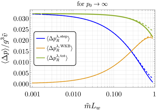
Figure 10: Analytically derived exact formulae for the exchanged momentum in the asymptotic limit $p^{0}\rightarrow\infty$ from emission of $\lambda$ polarisations. Dashed lines corresponds to the small $\tilde{m}L_{w}$ approximations reported in eq. 219. The sum of the two different contributions is roughly constant.

E.5 Vectors: $\lambda$ emission

We report again the relevant amplitudes here with general $v\neq 0$ :

$$\mathcal{M}^{\rm step}_{\lambda,L} =-i\frac{g}{E}(p^{z}+q^{z})\left[gv\left(\frac{1}{\Delta p_{r}}+\frac{r^{\lambda}_{k}}{\Delta p}\right)-g\tilde{v}\frac{t^{\lambda}_{k}}{\Delta\tilde{p}_{r}}\right]\ ,$$ (216)

$$\mathcal{M}^{\rm step}_{\lambda,R} =-i\frac{g}{E}(p^{z}+q^{z})\sqrt{k^{z}\over\tilde{k}^{z}}\left[gv\frac{\tilde{k}^{z}}{k^{z}}\frac{t^{\lambda}_{k}}{\Delta p}-g\tilde{v}\left(\frac{1}{\Delta\tilde{p}}-\frac{r^{\lambda}_{k}}{\Delta\tilde{p}_{r}}\right)\right]\ ,$$ (217)

$$\mathcal{M}^{\rm wkb\ red.}_{\lambda} =-i\frac{g}{E}(p^{z}+q^{z})\left[{gv\over\Delta p^{z}}-{g\tilde{v}\over\Delta\tilde{p}^{z}}\right]\ .$$ (218)

Unlike the case of $\tau$ we must consider the two transitions of interest separately.

Symmetric to Broken ($v=0$):

The symmetric side mass of the $\lambda$ degree of freedom is $m_{h,s}$ - the mass of the Higgs in that phase. We find however that taking $m_{h,s}=0$ incurs an error which is at most $\sim 10\%$ when $m_{h,s}\sim{\rm few}\>\times\tilde{m}$. One can rigorously prove that in the limit $p^{0}\rightarrow\infty$ we have

$$\langle\Delta p_{R}^{\lambda,\rm step}\rangle\longrightarrow \quad{g^{3}v^{2}\over 8\pi^{2}\tilde{m}}\;F^{\rm step}_{\lambda,R}(\tilde{m}L_{w})$$ (219)

$$= \quad{g^{3}v^{2}\over 8\pi^{2}\tilde{m}}\left[{2+4G-\pi}+\tilde{m}L_{w}\left(2\ln(\tilde{m}L_{w})-2\ln(2)-1\right)\right]+\mathcal{O}\left((\tilde{m}L_{w})^{3}\right)\ ,$$

$$\langle\Delta p_{R}^{\lambda,\rm wkb}\rangle\longrightarrow \quad{g^{3}v^{2}\over 8\pi^{2}\tilde{m}}\left[\tan^{-1}\left(\tilde{m}L_{w}\over\sqrt{1-\tilde{m}^{2}L_{w}^{2}}\right)-\tilde{m}L\ln\left(1-\sqrt{1-\tilde{m}^{2}L_{w}^{2}}\right)\right]\ ,$$ (220)

where $G\approx 0.916$ is Catalan’s constant. $F^{\rm step}_{\lambda,R}$ has a closed form in terms of (hyperbolic) trig functions and the dilogarithm, but we have deemed it more useful to explicitly report only its small $\tilde{m}L_{w}$ limit - an excellent approximation, as can be seen in fig. 10. There we also see that the sum of the two contributions is roughly constant, giving

$$\langle\Delta p^{\lambda,\rm total}\rangle\approx\langle\Delta p_{R}^{\lambda,\rm step}\rangle+\langle\Delta p_{R}^{\lambda,\rm wkb}\rangle\simeq{g^{3}v^{2}\over 8\pi^{2}\tilde{m}}\left[2+4G-\pi-\tilde{m}L_{w}\ln(2)\right]\ ,$$ (221)

to leading orders in $\tilde{m}L_{w}$. A more accurate expression when $\tilde{m}L_{w}\sim 1$ is eq. 220.

Appendix F Pressure in the EW phase transition

In this work we computed the pressure in the context of an Abelian toy model, where the $U(1)$ gauge boson was emitted by a complex scalar. Emission from fermions will not significantly change our result per degree of freedom. Moreover, the emission can be straightforwardly expanded to the non-Abelian case.

For the SM case, the pressure at $1\to 2$ level originates from the vertices inducing $\psi\to Z\psi$ (where the first particle in the final state is soft and $\psi$ is some fermion of the SM), $\psi\to W^{\pm}\psi$ for the gauge bosons emitted from fermions $H\to W^{\pm}H$, $H\to ZH$ for the gauge bosons emitted from the Higgs and $A\to WW,W\to WA$, $Z\to WW,W\to WZ,W\to ZW$ for gauge bosons emitting gauge bosons. The careful counting of all the processes involved in the pressure was presented in Appendix C of [45]. This leads to final pressure of the form

$$\mathcal{P}_{\text{SM},1\to 2}\approx 157\times\alpha_{\rm em}M_{Z}\frac{4\gamma_{w}\zeta(3)T^{3}}{\pi}\bigg{[}0.135\log\left(\frac{\tilde{v}}{T}+2.26\right)$$

$$-0.085-0.2\frac{\log\left(\frac{\tilde{v}}{T}+2.26\right)}{\tilde{v}/T}+\frac{0.19}{\tilde{v}/T}\bigg{]}\ ,$$ (222)

where every contribution has is normalised to the fine structure constant $\alpha_{\rm em}$ and the $Z$ boson mass $M_{Z}$ in broken phase. We caution the reader that this expression is still an estimate and may incur future revision, for example, from a better understanding of finite temperature corrections - see section 4.2.

Appendix G Sensitivity to wall width

In this work we separated the phase space of particles according to when the step wall and WKB approximations are justified

• $k^{z}<L_{w}^{-1}$,    Step wall

• $k^{z}>L_{w}^{-1}$,    WKB

where $L_{w}$ is the width of the wall. However, this is a somewhat arbitrary quantity, significant up to some order 1 factor. Although we have discussed the sensitivity of our results to $L_{w}$ in several places, we summarise it in this dedicated appendix.

We study numerically how pressure changes with wall width. For scalars, the dominant contribution comes from the WKB regime and dependence on $L_{w}$ vanishes, as can be seen in explicitly by the analytical formulae eqs. 51 and 207. The results for vector emission are highlighted in fig. 11. The left and right columns show left and right mover emission respectively, while top and lower panels correspond to $\tau$ and $\lambda$ polarisations. The first thing to notice is that $\langle{\Delta p_{L}^{\tau,\,\rm step}}\rangle$, which is the dominant contribution for super-cooled symmetric to broken transitions is largely insensitive to $L_{w}$. Secondly, $\langle{\Delta p_{R}^{\lambda,\,\rm step}}\rangle$ and $\langle{\Delta p_{R}^{\lambda,\,\rm wkb}}\rangle$ show almost linear dependence around $L_{w}\sim{\rm few}\;\tilde{m}$ but their sum is largely constant. This point was made also in fig. 10 using analytical asymptotic formulae. Instead, $\langle{\Delta p_{L}^{\lambda,\,\rm step}}\rangle$, which exists only in broken to broken transitions is linearly dependent on the cut-off (see eq. (152)).

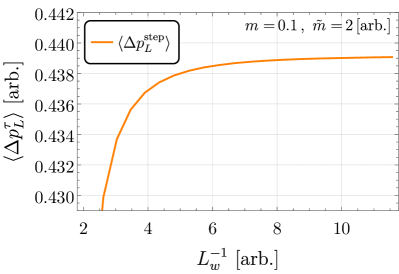
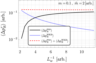
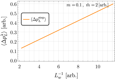
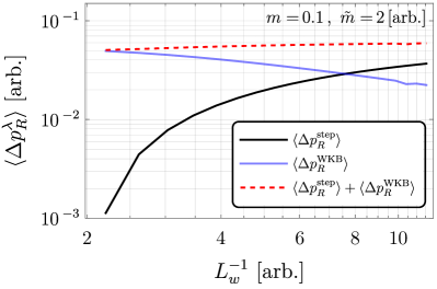
Figure 11: Dependence of various contributions to average momentum transfer, due to the emission of a vector boson, on the inverse wall width $L_{w}^{-1}$ in the limit $p_{0}\to\infty$. Top (Bottom) panels refers to $\tau$ ($\lambda$) emission, while left (right) column refers to $L$ ($R$) emission. In this limit, any dependence on the mass of the emitter ($m_{\psi}$) vanishes.

Appendix H The suppressed region $\Delta p_{z}L_{w}\gg 1$: the Fourier constraint

In section 2.6 and afterwards, we stated that in WKB approximation the region $\Delta p_{z}L_{w}\gg 1$ should have a very suppressed contribution to the pressure. In this appendix, we bring some arguments to this claim (see also Appendix B.1 of [66] and Section V of [63] for previous discussion). The function that we have to study is typically the following integral

$$\mathcal{M}\approx\int^{\infty}_{-\infty}dzV(z)e^{i\int^{z}_{-\infty}\Delta p_{z}(z^{\prime})dz^{\prime}}\,,$$ (223)

where far from the wall both $\Delta p(z)$ and $V(z)$ are constant. In this case we can always absorb $V(z)=V_{0}\exp[\int_{0}^{z}(V^{\prime}/V)dz]$ inside the exponent (redefining $\Delta p$) and thus we can focus only on the integrals where $V(z)=V_{0}$

$$\mathcal{M}\approx V_{0}\int^{\infty}_{-\infty}dze^{i\int^{z}_{0}\Delta p_{z}(z^{\prime})dz^{\prime}}\,.$$ (224)

In general these integrals must be evaluated numerically for various wall shapes. However for particular choice like

$$\Delta p_{z}(z)=\Delta p_{z}+\frac{\epsilon}{2}\tanh{z/L_{w}},$$ (225)

we can evaluate the integrals analytically. In eq. 225, $\epsilon$ parameterises the change of the phase across the wall. This leads to

$$\mathcal{M} =V_{0}\int^{\infty}_{-\infty}dz\exp\left[i\Delta p_{z}z+i\epsilon f(z)\right],$$

$$f(z) =\frac{L_{w}}{2}\log\cosh{\frac{z}{L_{w}}}\,,$$ (227)

and give finally

$$|\mathcal{M}|^{2} =\frac{\pi\epsilon L_{w}|V_{0}|^{2}}{2\Delta p_{z}^{2}-\epsilon^{2}/2}\times\frac{\sinh{(\pi\epsilon L_{w}/2)}}{\sinh{(\pi(\Delta p_{z}-\epsilon/2)L_{w}/2)}\sinh{(\pi(\Delta p_{z}+\epsilon/2)L_{w}/2)}}$$

$$\approx\frac{\pi\epsilon L_{w}|V_{0}|^{2}}{2\Delta p_{z}^{2}}\times\frac{\sinh{(\pi\epsilon L_{w}/2)}}{\sinh^{2}{(\pi\Delta p_{z}L_{w}/2)}}\,.$$ (229)

For $\epsilon L_{w}\lesssim 1,\Delta p_{z}L_{w}\gg 1$, we obtain

$$|\mathcal{M}|^{2}\approx\frac{\pi\epsilon L_{w}|V_{0}|^{2}}{4\Delta p_{z}^{2}}\times\pi\epsilon L_{w}e^{-\pi\Delta p_{z}L_{w}}=\frac{(\pi\epsilon L_{w})^{2}|V_{0}|^{2}}{4\Delta p_{z}^{2}}\times e^{-\pi\Delta p_{z}L_{w}}$$ (230)

which shows that $|\mathcal{M}|^{2}\propto e^{-\pi\Delta p_{z}L_{w}}$ and then decay exponentially with $\Delta p_{z}L_{w}\gg 1$. We have also checked numerically the behaviour of the amplitude for other wall shapes, with a similar behaviour (for example Erf function) and always find exponential suppression.

References

- [1] D. A. Kirzhnits and A. D. Linde Phys. Lett. 42B: No. 4, 471-4(25 Dec 1972). (1, 1972).
- [2] S. Weinberg Phys. Rev. D 9 (Jun, 1974) 3357–3378.
- [3] E. Witten Phys. Rev. D30 (1984) 272–285.
- [4] C. Bonati, M. D’Elia, P. de Forcrand, O. Philipsen, and F. Sanfilippo PoS LATTICE2013 (2014) 219, [arXiv:1311.0473].
- [5] M. Laine and K. Rummukainen Nucl. Phys. B Proc. Suppl. 73 (1999) 180–185, [hep-lat/9809045].
- [6] G. Degrassi, S. Di Vita, J. Elias-Miro, J. R. Espinosa, G. F. Giudice, G. Isidori, and A. Strumia JHEP 08 (2012) 098, [arXiv:1205.6497].
- [7] V. A. Kuzmin, V. A. Rubakov, and M. E. Shaposhnikov Phys. Lett. B 155 (1985) 36.
- [8] M. Shaposhnikov JETP Lett. 44 (1986) 465–468.
- [9] A. E. Nelson, D. B. Kaplan, and A. G. Cohen Nucl. Phys. B 373 (1992) 453–478.
- [10] M. Carena, M. Quiros, and C. E. M. Wagner Phys. Lett. B 380 (1996) 81–91, [hep-ph/9603420].
- [11] J. M. Cline Phil. Trans. Roy. Soc. Lond. A 376 (2018), no. 2114 20170116, [arXiv:1704.08911].
- [12] A. J. Long, A. Tesi, and L.-T. Wang JHEP 10 (2017) 095, [arXiv:1703.04902].
- [13] S. Bruggisser, B. Von Harling, O. Matsedonskyi, and G. Servant JHEP 12 (2018) 099, [arXiv:1804.07314].
- [14] S. Bruggisser, B. Von Harling, O. Matsedonskyi, and G. Servant Phys. Rev. Lett. 121 (2018), no. 13 131801, [arXiv:1803.08546].
- [15] D. E. Morrissey and M. J. Ramsey-Musolf New J. Phys. 14 (2012) 125003, [arXiv:1206.2942].
- [16] A. Azatov, M. Vanvlasselaer, and W. Yin JHEP 10 (2021) 043, [arXiv:2106.14913].
- [17] I. Baldes, S. Blasi, A. Mariotti, A. Sevrin, and K. Turbang arXiv:2106.15602.
- [18] E. J. Chun, T. P. Dutka, T. H. Jung, X. Nagels, and M. Vanvlasselaer arXiv:2305.10759.
- [19] A. Falkowski and J. M. No JHEP 02 (2013) 034, [arXiv:1211.5615].
- [20] I. Baldes, Y. Gouttenoire, and F. Sala JHEP 04 (2021) 278, [arXiv:2007.08440].
- [21] A. Azatov, M. Vanvlasselaer, and W. Yin JHEP 03 (2021) 288, [arXiv:2101.05721].
- [22] I. Baldes, Y. Gouttenoire, F. Sala, and G. Servant JHEP 07 (2022) 084, [arXiv:2110.13926].
- [23] P. Asadi, E. D. Kramer, E. Kuflik, G. W. Ridgway, T. R. Slatyer, and J. Smirnov Phys. Rev. D 104 (2021), no. 9 095013, [arXiv:2103.09827].
- [24] I. Baldes, Y. Gouttenoire, and F. Sala SciPost Phys. 14 (2023) 033, [arXiv:2207.05096].
- [25] I. Baldes, M. Dichtl, Y. Gouttenoire, and F. Sala arXiv:2306.15555.
- [26] H. Kodama, M. Sasaki, and K. Sato Progress of Theoretical Physics 68 (12, 1982) 1979–1998, [https://academic.oup.com/ptp/article-pdf/68/6/1979/5311817/68-6-1979.pdf].
- [27] K. Kawana and K.-P. Xie Phys. Lett. B 824 (2022) 136791, [arXiv:2106.00111].
- [28] T. H. Jung and T. Okui arXiv:2110.04271.
- [29] Y. Gouttenoire and T. Volansky arXiv:2305.04942.
- [30] M. Lewicki, P. Toczek, and V. Vaskonen arXiv:2305.04924.
- [31] C. J. Hogan Mon. Not. Roy. Astron. Soc. 218 (1986) 629–636.
- [32] A. Kosowsky and M. S. Turner Phys. Rev. D47 (1993) 4372–4391, [astro-ph/9211004].
- [33] A. Kosowsky, M. S. Turner, and R. Watkins Phys. Rev. Lett. 69 (1992) 2026–2029.
- [34] M. Kamionkowski, A. Kosowsky, and M. S. Turner Phys. Rev. D49 (1994) 2837–2851, [astro-ph/9310044].
- [35] C. Grojean, G. Servant, and J. D. Wells Phys. Rev. D 71 (2005) 036001, [hep-ph/0407019].
- [36] C. Delaunay, C. Grojean, and J. D. Wells JHEP 04 (2008) 029, [arXiv:0711.2511].
- [37] J. Ellis, M. Lewicki, and J. M. No arXiv:1809.08242. [JCAP1904,003(2019)].
- [38] J. Ellis, M. Lewicki, J. M. No, and V. Vaskonen JCAP 1906 (2019), no. 06 024, [arXiv:1903.09642].
- [39] J. R. Espinosa and M. Quiros Phys. Rev. D 76 (2007) 076004, [hep-ph/0701145].
- [40] A. Beniwal, M. Lewicki, J. D. Wells, M. White, and A. G. Williams JHEP 08 (2017) 108, [arXiv:1702.06124].
- [41] V. Barger, P. Langacker, M. McCaskey, M. J. Ramsey-Musolf, and G. Shaughnessy Phys. Rev. D 77 (2008) 035005, [arXiv:0706.4311].
- [42] J. R. Espinosa, T. Konstandin, and F. Riva Nucl. Phys. B 854 (2012) 592–630, [arXiv:1107.5441].
- [43] J. Kozaczuk, M. J. Ramsey-Musolf, and J. Shelton Phys. Rev. D 101 (2020), no. 11 115035, [arXiv:1911.10210].
- [44] G. Kurup and M. Perelstein Phys. Rev. D 96 (2017), no. 1 015036, [arXiv:1704.03381].
- [45] A. Azatov, G. Barni, S. Chakraborty, M. Vanvlasselaer, and W. Yin JHEP 10 (2022) 017, [arXiv:2207.02230].
- [46] I. Garcia Garcia, S. Krippendorf, and J. March-Russell Phys. Lett. B 779 (2018) 348–352, [arXiv:1607.06813].
- [47] J. R. Espinosa, T. Konstandin, J. M. No, and G. Servant JCAP 1006 (2010) 028, [arXiv:1004.4187].
- [48] R. Jinno and M. Takimoto JCAP 1901 (2019) 060, [arXiv:1707.03111].
- [49] M. Fairbairn, E. Hardy, and A. Wickens JHEP 07 (2019) 044, [arXiv:1901.11038].
- [50] M. Breitbach, J. Kopp, E. Madge, T. Opferkuch, and P. Schwaller JCAP 07 (2019) 007, [arXiv:1811.11175].
- [51] G. D. Moore and T. Prokopec Phys. Rev. Lett. 75 (1995) 777–780, [hep-ph/9503296].
- [52] G. D. Moore and T. Prokopec Phys. Rev. D52 (1995) 7182–7204, [hep-ph/9506475].
- [53] B. Laurent and J. M. Cline Phys. Rev. D 106 (2022), no. 2 023501, [arXiv:2204.13120].
- [54] B. Laurent and J. M. Cline Phys. Rev. D 102 (2020), no. 6 063516, [arXiv:2007.10935].
- [55] S. De Curtis, L. D. Rose, A. Guiggiani, A. G. Muyor, and G. Panico arXiv:2201.08220.
- [56] S. De Curtis, L. Delle Rose, A. Guiggiani, A. Gil Muyor, and G. Panico JHEP 05 (2023) 194, [arXiv:2303.05846].
- [57] M. Barroso Mancha, T. Prokopec, and B. Swiezewska arXiv:2005.10875.
- [58] S. Balaji, M. Spannowsky, and C. Tamarit JCAP 03 (2021) 051, [arXiv:2010.08013].
- [59] W.-Y. Ai, B. Garbrecht, and C. Tamarit arXiv:2109.13710.
- [60] W.-Y. Ai, B. Laurent, and J. van de Vis arXiv:2303.10171.
- [61] M. Dine, R. G. Leigh, P. Y. Huet, A. D. Linde, and D. A. Linde Phys. Rev. D46 (1992) 550–571, [hep-ph/9203203].
- [62] D. Bodeker and G. D. Moore JCAP 0905 (2009) 009, [arXiv:0903.4099].
- [63] D. Bodeker and G. D. Moore JCAP 1705 (2017), no. 05 025, [arXiv:1703.08215].
- [64] S. Höche, J. Kozaczuk, A. J. Long, J. Turner, and Y. Wang JCAP 03 (2021) 009, [arXiv:2007.10343].
- [65] A. Azatov and M. Vanvlasselaer JHEP 09 (2020) 085, [arXiv:2003.10265].
- [66] Y. Gouttenoire, R. Jinno, and F. Sala JHEP 05 (2022) 004, [arXiv:2112.07686].
- [67] M. Barroso Mancha, T. Prokopec, and B. Swiezewska JHEP 01 (2021) 070, [arXiv:2005.10875].
- [68] I. Garcia Garcia, G. Koszegi, and R. Petrossian-Byrne arXiv:2212.10572.
- [69] A. Azatov and M. Vanvlasselaer JCAP 01 (2021) 058, [arXiv:2010.02590].
- [70] G. R. Farrar and J. W. McIntosh, Jr. Phys. Rev. D 51 (1995) 5889–5904, [hep-ph/9412270].
- [71] A. Shkerin and S. Sibiryakov JHEP 11 (2021) 197, [arXiv:2105.09331].
- [72] M. E. Peskin and D. V. Schroeder, An Introduction to quantum field theory. Addison-Wesley, Reading, USA, 1995.
- [73] M. L. Bellac, Thermal Field Theory. Cambridge Monographs on Mathematical Physics. Cambridge University Press, 3, 2011.