Positivity-free Policy Learning with Observational Data

Abstract

Policy learning utilizing observational data is pivotal across various domains, with the objective of learning the optimal treatment assignment policy while adhering to specific constraints such as fairness, budget, and simplicity. This study introduces a novel positivity-free (stochastic) policy learning framework designed to address the challenges posed by the impracticality of the positivity assumption in real-world scenarios. This framework leverages incremental propensity score policies to adjust propensity score values instead of assigning fixed values to treatments. We characterize these incremental propensity score policies and establish identification conditions, employing semiparametric efficiency theory to propose efficient estimators capable of achieving rapid convergence rates, even when integrated with advanced machine learning algorithms. This paper provides a thorough exploration of the theoretical guarantees associated with policy learning and validates the proposed framework’s finite-sample performance through comprehensive numerical experiments, ensuring the identification of causal effects from observational data is both robust and reliable.

Keywords: incremental propensity score intervention, individualized treatment rule, natural stochastic policy, off-policy learning, semiparametric efficiency

1 Introduction

Over the past decade, methodologies for learning treatment assignment policies have seen substantial advancements in fields like biostatistics (Luedtke and van der Laan, 2016b; Tsiatis et al., 2019), computer science (Uehara et al., 2022; Yu et al., 2022), and econometrics (Athey and Wager, 2021; Jia et al., 2023). The core objective of data-driven policy learning is to learn optimal policies that map individual characteristics to treatment assignments to optimize some utility or outcome functions. This is crucial for deriving robust and trustworthy policies in high-stakes decision-making settings, requiring adherence to standard causal assumptions: consistency, unconfoundedness, and positivity (van der Laan et al., 2011; Imbens and Rubin, 2015).

Various statistical and machine-learning methods have been developed to address policy learning tasks. Popular approaches include model-based methods such as Q-learning and A-learning (Murphy, 2003; Shi et al., 2018), and direct model-free policy search methods such as decision trees and outcome weighted learning (Zhang et al., 2012; Cui et al., 2017), among others (Bibaut et al., 2021; Zhou et al., 2023). Another prevailing line of work concerns heterogeneous treatment effects estimation (Wager and Athey, 2018; Künzel et al., 2019; Nie and Wager, 2021; Kallus and Oprescu, 2023), where the sign of the conditional average treatment effects equivalently determines the optimal policy.

However, most methods depend heavily on the three standard causal assumptions to identify causal effects and optimal policies. Recent progress has been made to relax the consistency and unconfoundedness assumptions (Cortez et al., 2022; Kallus and Zhou, 2018), but advancements addressing the violation of the positivity assumption are scarce. Yang and Ding (2018) and Branson et al. (2023) provide estimation and asymptotic inference results for propensity score trimming with binary and continuous treatments. Lawrence et al. (2017) consider counterfactual learning from deterministic bandit logs under lack of sufficient exploration. Gui and Veitch (2023) use supervised representation learning to estimate causal effects for text data with apparent overlap violation. Zhang et al. (2023) consider a missing-at-random mechanism without a positivity condition for generalizable and double robust inference for average treatment effects under selection bias with decaying overlap. Jin et al. (2022) use pessimism and generalized empirical Bernstein’s inequality to study offline policy learning without assuming any uniform overlap condition. Khan et al. (2023) provide partial identification results for off-policy evaluation under non-parametric Lipschitz smoothness assumptions on the conditional mean function, and thus avoid assuming either overlap or a well-specified model. Liu et al. (2023) propose the overlap weighted average treatment effect on the treated under lack of positivity. To our knowledge, our work is the first to consider learning treatment assignment policies while avoiding the positivity assumption.

This study introduces a novel positivity-free policy learning framework focusing on dynamic and stochastic policies, which are practical. We propose incremental propensity score policies that shift propensity scores by an individualized parameter, requiring only the consistency and unconfoundedness causal assumptions. Our approach enhances the concept of incremental intervention effects, as proposed by Kennedy (2019), adapting it to individual treatment policy contexts.

We also use semiparametric theory to characterize the efficient influence function (Bickel et al., 1993; van der Laan and Robins, 2003), which serves as the foundation to construct estimators with favorable properties, such as double/multiple robustness and asymptotically negligible second-order bias (also called Neyman orthogonality in double machine learning (Chernozhukov et al., 2018) or orthogonal statistical learning (Foster and Syrgkanis, 2023)). Thus, our proposed estimators can attain fast parametric $\sqrt{n}$ convergence rates, even when nuisance parameters are estimated at slower rates such as $n^{1/4}$ via flexible machine learning algorithms.

Based on the above efficient off-policy evaluation results, we propose approaches to learning the optimal policy by maximizing the value function, possibly under application-specific constraints. Several examples are provided in Section 4, including fairness and resource limit. While it remains an open problem to provide finite sample or asymptotic regret bounds as Athey and Wager (2021) for stochastic policy learning with constraints, which is out of the scope of this article, we establish asymptotic guarantees for our proposed policy learning methods under alternative (stronger) conditions.

The rest of this article is organized as follows. Section 2 introduces the basic setup and notations and proposes the incremental propensity score policy. Our main identification and semiparametric efficiency theory results for off-policy evaluation are presented in Section 3. Section 4 formally introduces our positivy-free policy learning framework, with several examples. Asymptotic analysis of guarantees for policy evaluation and learning are given in Section 5. Finally, we illustrate our methods via simulations and a data application in Section 6. The article concludes in Section 7 with a discussion of some remarks and future work. All proofs and additional results are provided in the Supplementary Material.

2 Statistical Framework

We first introduce the notations and setup. Let $X$ denote the $p$-dimensional vector of covariates that belongs to a covariate space $\mathcal{X}\subset\mathbb{R}^{p}$, $A\in\mathcal{A}=\{0,1\}$ denote the binary treatment, $Y\in\mathbb{R}$ denote the outcome of interest. Without loss of generality, we assume throughout that larger values of $Y$ are more desirable. Our observed data structure is $O=(X,A,Y)$. Suppose that our collected random sample $(O_{1},\ldots,O_{n})$ of size $n$ are independent and identically distributed (i.i.d.) observations of $O\sim P$, where $P$ denote the true distribution of the observed data.

Now, we are in the position to introduce different types of policies or interventions commonly used in the literature: (i) under static policies, the same treatments would be applied indiscriminately, while dynamic policies depend on individual characteristics; (ii) deterministic policies recommend one specific treatment and stochastic policies output probabilities of prescribing each treatment level. This article focuses on dynamic and stochastic policies, which are more practical in various settings and have received substantial recent interest. Typical examples include point exposures (Dudík et al., 2014), longitudinal studies (Tian, 2008; Murphy et al., 2001; van der Laan and Petersen, 2007), natural stochastic policies in reinforcement learning (Kallus and Uehara, 2020), and particularly interventions that depend on the observational treatment process (Muñoz and van Der Laan, 2012; Haneuse and Rotnitzky, 2013; Young et al., 2014); but none of the existing intervention effects both avoids positivity conditions entirely and is completely nonparametric.

We use the potential outcomes framework (Neyman, 1923; Rubin, 1974) to define causal effects. Let $Y(a)$ denote the potential outcome had the treatment $a$ been assigned. A policy $d:\mathcal{X}\to\{0,1\}$ is deterministic if it maps individual characteristics $x$ to a treatment assignment $0$ or $1$, and the output of a stochastic policy $d:\mathcal{X}\to[0,1]$ is the probability of assigning treatment $1$. Let $\mathcal{D}$ denote a pre-specified class of policies of interest, where each policy $d\in\mathcal{D}$ induces the value function defined by

$$V(d)=E[Y(d)]=E[Y(1)d(X)+Y(0)(1-d(X))],$$

where $Y(d)$ is the potential outcome under the policy $d$. In Remark 1, we briefly review standard (deterministic) policy learning methods. In our framework, we focus on dynamic and stochastic policies. Our goal is to directly search for the optimal policy $d^{\ast}$ that maximizes the value function $V(d)$, possibly under application-specific constraints $c(d)\leq 0$. See Section 4 for detailed examples.

2.1 Causal Assumptions

We make the following identification assumptions.

Assumption 1 (Consistency).

$Y=Y(A)$.

Assumption 2 (Unconfoundedness).

$A\perp Y(a)\mid X$ for $a=0,1$.

Assumption 1 is also known as the stable unit treatment value assumption, which says there should be no multiple versions of the treatment and no interference between units. Assumption 2 states that there are no unmeasured confounders so that treatment assignment is as good as random conditional on the covariates $X$. In this article, we entirely avoid the positivity assumption which requires that each unit has a positive probability of receiving both treatment levels, i.e., $c<Pr(A=1\mid X)<1-c$ for some constant $c>0$.

Remark 1.

Standard policy learning methods need all of Assumptions 1, 2 and the positivity assumption to identify the value function of deterministic policies $d:\mathcal{X}\to\mathcal{A}$ by the outcome regression (OR), inverse probability weighting (IPW) and augmented IPW (AIPW) formulas:

$$V_{\rm OR}(d) =E[E[Y\mid X,A=d(X)]],\quad V_{\rm IPW}(d)=E\left[\frac{I\{A=d(X)\}Y}{Pr(A=d(X)\mid X)}\right],$$

$$V_{\rm AIPW}(d) =E\left[E[Y\mid X,A=d(X)]+\frac{I\{A=d(X)\}(Y-E[Y\mid X,A=d(X)])}{Pr(A=d(X)\mid X)}\right],$$

thus the optimal policies are given by $d_{\rm OR}^{\ast}=\arg\max_{d\in\mathcal{D}}V_{\rm OR}(d)$, $d_{\rm IPW}^{\ast}=\arg\max_{d\in\mathcal{D}}V_{\rm IPW}(d)$, and $d_{\rm AIPW}^{\ast}=\arg\max_{d\in\mathcal{D}}V_{\rm AIPW}(d)$, possibly under application-specific constraints. When the positivity is violated, it is error-prone to rely on the outcome regression model’s extrapolation, and the IPW and AIPW estimators would fail due to division by zero.

2.2 Incremental Propensity Score Policies

Kennedy (2019) propose a new class of stochastic dynamic intervention, called incremental propensity score interventions, and show that these interventions are nonparametrically identified without requiring any positivity restrictions on the propensity scores. Specifically, their proposed intervention replaces the observational propensity score $\pi$ with a shifted version based on multiplying the odds of receiving treatment, ${\delta\pi(x)}/\{\delta\pi(x)+1-\pi(x)\}$, where the increment parameter $\delta\in(0,\infty)$ is user-specified and dictates the extent to which the propensity scores fluctuate from their actual observational values. Some motivation and examples, efficiency theory, and estimators for mean outcomes under these interventions are studied in detail by Kennedy (2019).

We propose a positivity-free (stochastic) policy learning framework based on the incremental propensity score interventions. Specifically, we consider the stochastic policy $d:\mathcal{X}\to[0,1]$ that assigns treatment $1$ with probability

$$d(x)=\frac{\delta(x)\pi(x)}{\delta(x)\pi(x)+1-\pi(x)},$$ (1)

where $\delta(x)$ enables individualized treatment assignment. We note that the choice of $d(x)$ in (1) is motivated by its interpretability and positivity-free. In particular, whenever $0<\pi(x)<1$, $\delta(x)=[{d(x)/\{1-d(x)\}}]/[\pi(x)/\{1-\pi(x)\}]$ is simply an odds ratio, indicating how the policy changes the odds of receiving treatment. When positivity is violated, we have that $d(x)=0$ if $\pi(x)=0$, and $d(x)=1$ if $\pi(x)=1$.

3 Identification and Efficiency Theory

3.1 Identification

We first give formal identification results for the value function of incremental propensity score policies, which require no conditions on the propensity scores.

Proposition 1 (Identification formulas).

Under Assumptions 1 and 2, the value function $V(d)$ can be nonparametrically identified by the outcome regression with incremental propensity score (OR-IPS) formula:

$$V_{\rm OR-IPS}(d)=E\left[\frac{\delta(X)\pi(X)\mu_{1}(X)+\{1-\pi(X)\}\mu_{0}(X)}{\delta(X)\pi(X)+1-\pi(X)}\right],$$ (2)

where $\mu_{a}(X)=E[Y\mid X,A=a],a=0,1$ are the outcome regression functions or the inverse probability weighting of incremental propensity score (IPW-IPS) formula:

$$V_{\rm IPW-IPS}(d)=E\left[\frac{Y\{\delta(X)A+1-A\}}{\delta(X)\pi(X)+1-\pi(X)}\right].$$ (3)

Proposition 1 shows that the value function can be identified by (i) a weighted average of the outcome regression functions $\mu_{0},\mu_{1}$, where the weight on $\mu_{1}$ is given by the incremental propensity score $d(x)$ and the weight on $\mu_{0}$ is $1-d(x)$; (ii) inverse probability weighting where each treated is weighted by the (inverse of the) propensity score plus some fractional contribution of its complement, i.e., $\pi(x)+(1-\pi(x))/\delta(x)$, and untreated units are weighted by this same amount, except the entire weight is further down-weighted by a factor of $\delta(x)$.

3.2 Efficient Off-policy Evaluation

Despite that simple plug-in OR-IPS and IPW-IPS estimators can be easily constructed from (2) and (3), these estimators will only be $\sqrt{n}$-consistent when the outcome regression or propensity score models are correctly specified. This is usually unrealistic in practice. We use semiparametric efficiency theory to study the following statistical functional of $P$ from a nonparametric statistical model $\mathcal{M}$:

$$\Psi(P)=V(d)=E_{P}\left[\frac{\delta(X)\pi(X)\mu_{1}(X)+\{1-\pi(X)\}\mu_{0}(X)}{\delta(X)\pi(X)+1-\pi(X)}\right],$$

and propose efficient estimators based on the efficient influence function.

Proposition 2 (Semiparametric Efficiency).

The efficient influence function of $\Psi(P)$ is

$$\begin{split}\phi(P)(O)&=\frac{A\delta(X)\{Y-\mu_{1}(X)\}+(1-A)\{Y-\mu_{0}(X)\}+\delta(X)\pi(X)\mu_{1}(X)+\{1-\pi(X)\}\mu_{0}(X)}{\delta(X)\pi(X)+1-\pi(X)}\\ &\quad+\frac{\delta(X)\tau(X)\{A-\pi(X)\}}{\{\delta(X)\pi(X)+1-\pi(X)\}^{2}}-\Psi(P),\end{split}$$ (4)

where $\tau(x)=\mu_{1}(x)-\mu_{0}(x)$.

By Proposition 2, the one-step bias-corrected estimator is given by

$$\hat{\Psi}_{\rm OS}=\Psi(\hat{P})+P_{n}\phi(\hat{P})(O)=\frac{1}{n}\sum_{i=1}^{n}\xi(\hat{P})(O_{i}),$$ (5)

where we estimate $P$ by $\hat{P}$, and let $P_{n}$ denote the empirical distribution, and $\xi(P)(O)=\phi(P)(O)+\Psi(P)$ is the uncentered efficient influence function. This estimator can converge at fast parametric $\sqrt{n}$ rates and attain the efficiency bound, even when the propensity score $\pi(x)$ and outcome regression functions $\mu_{0},\mu_{1}$ are modeled flexibly and estimated at rates slower than $\sqrt{n}$, as long as these nuisance functions are estimated consistently at rates faster than $n^{1/4}$. This allows much more flexible nonparametric methods and modern machine learning algorithms to be employed.

However, characterizing asymptotic properties of the estimator (5) requires some empirical process conditions that restrict the flexibility and complexity of the nuisance estimators; otherwise, we will have overfitting bias and intractable asymptotic behaviors. See the asymptotic analysis in Section 5 and proofs thereof. To accommodate the wide use of modern machine learning algorithms that usually fail to satisfy the required empirical process conditions, we apply the cross-fitting procedure to obtain asymptotically normal and efficient estimators (Zheng and van der Laan, 2010; Chernozhukov et al., 2018). Suppose we randomly split the data into $K$ folds. Then the cross-fitting estimator is

$$\hat{\Psi}_{\rm CF}=\frac{1}{K}\sum_{k=1}^{K}\hat{\Psi}_{k}=\frac{1}{K}\sum_{k=1}^{K}P_{n,k}\xi(P_{n,-k})(O),$$ (6)

where $P_{n,k}$ and $P_{n,-k}$ denote the empirical measures on data from the $k$-fold and excluding the $k$-fold, respectively. That is, for $k=1,\ldots,K$, nuisance estimators are constructed excluding the $k$-fold, and the value function $\hat{\Psi}_{k}$ is evaluated on the $k$-th fold; finally, the cross-fitting estimator is the average of the $K$ value estimators from $K$ folds.

4 From Efficient Policy Evaluation to Learning

In this section, we first present our proposed methods for policy learning.

As discussed in Section 2, given a pre-specified policy class $\mathcal{D}$ (e.g., linear decision rules), we propose estimating the optimal treatment assignment rule $\hat{d}$ that solves (i) $\hat{d}=\arg\max_{d\in\mathcal{D}}\hat{V}(d)$, where $\hat{V}(d)$ is a value function estimator by OR-IPS (2), IPW-IPS (3), one-step (5) or cross-fitting (6); or (ii) $\hat{d}=\arg\max_{d\in\mathcal{D}}\hat{V}(d)$ subject to $\hat{c}(d)\leq c$, when an application-specific constraint $c(d)\leq c$ is imposed, and $\hat{c}(d)$ is a constraint estimator which usually needs to be studied on a case-by-case basis.

We first review important examples of policy learning that fit into our framework.

Vanilla direct policy search. The first example is what most existing work on policy learning has focused on, primarily for deterministic policies with a binary treatment. When the policy class is unrestricted, the optimal treatment assignment rule depends on the sign of the conditional average treatment effect for each individual unit, which cannot be extended to stochastic policies. Our proposed optimal incremental propensity score policies maximize the value function.

Fair policy learning. In many decision-making scenarios, such as hiring, recommendation systems, and criminal justice, concerns have been raised regarding the fairness of decisions from the learning process (Chzhen et al., 2020). Let $S\in\mathcal{S}$ denote the sensitive attribute. For randomized predictions $f:\mathcal{X}\times\mathcal{S}\to\Delta(\mathcal{A})$, popular fairness criteria include demographic parity (DP) (Calders et al., 2009):

$$E[f(X,S)\mid S=s]=E[f(X,S)\mid S=s^{\prime}],\forall s,s^{\prime}\in\mathcal{S},$$ (7)

which says that $f(X,S)$ is independent from $S$, or equal opportunity (EO) (Hardt et al., 2016):

$$E[f(X,S)\mid S=s,A=a]=E[f(X,S)\mid S=s^{\prime},A=a],\forall s,s^{\prime}\in\mathcal{S},a\in\mathcal{A},$$ (8)

which requires equal true positive and true negative rates. Following the same spirit, we consider fair policy learning tasks as the constrained optimization problem:

$$\max_{d\in\mathcal{D}}V(d),\text{ subject to }f(d)\leq b,$$

where $f(d)$ is either the DP or EO metrics, which can be estimated by

$$\hat{f}_{\rm DP}(d)=\left(\sum_{s\in\mathcal{S}}\left(\frac{\sum_{i=1}^{n}d(X_{i})I\{S_{i}=s\}}{\sum_{i=1}^{n}I\{S_{i}=s\}}-\frac{\sum_{i=1}^{n}d(X_{i})}{n}\right)^{2}\right)^{1/2},$$

or

$$\hat{f}_{\rm EO}(d)=\left(\sum_{s\in\mathcal{S}}\left(\frac{\sum_{i=1}^{n}d(X_{i})I\{S_{i}=s,A_{i}=1\}}{\sum_{i=1}^{n}I\{S_{i}=s,A_{i}=1\}}-\frac{\sum_{i=1}^{n}d(X_{i})I\{A_{i}=1\}}{\sum_{i=1}^{n}I\{A_{i}=1\}}\right)^{2}\right)^{1/2},$$

and $b$ is a pre-specified tuning parameter.

Resource-limited policy learning. In many real-world applications, the proportion of individuals who can receive the treatment is a priori limited due to a budget or a capacity constraint. So we consider the resource-limited policy learning tasks as the constrained optimization problem:

$$\max_{d\in\mathcal{D}}V(d),\text{ subject to }E[d]\leq b,$$

where $b$ is the pre-specified budget or capacity.

Protect the vulnerable. Since the optimal policy is typically defined as the maximizer of the expected potential outcome over the entire population, such a policy may be suboptimal or even detrimental to certain disadvantaged subgroups. Fang et al. (2022) propose the fairness-oriented optimal policy learning framework:

$$\max_{d\in\mathcal{D}}V(d),\text{ subject to }Q_{\tau}(Y(d))\geq b,$$

where $Q_{\tau}(Y(d))=\inf\{t:F_{Y(d)}(t)\geq\tau\}$ is the $\tau$-th quantile of $Y(d)$, $F_{Y(d)}$ denotes the cumulative distribution function of $Y(d)$, and $b$ is a pre-specified protection threshold. Note that the quantile function can be estimated by $\hat{Q}_{\tau}(Y(d))=\arg\min_{q}n^{-1}\sum_{i=1}^{n}c_{i}(d)\rho_{\tau}(Y_{i}-q)$, where $\rho_{\tau}(u)=u(\tau-I\{u<0\})$ is the quantile loss function, and $c_{i}(d)=A_{i}d(X_{i})+(1-A_{i})(1-d(X_{i}))$.

Other examples in the literature include the counterfactual no-harm criterion by the principal stratification method (Li et al., 2023), (weakly) NP-hard knapsack problem (Luedtke and van der Laan, 2016a), and instrumental variable methods (Qiu et al., 2021).

5 Asymptotic Analysis of Policy Evaluation and Learning

In this section, we first characterize the asymptotic distributions of our proposed one-step estimator (5) and the cross-fitted estimator (6) for off-policy evaluation.

Theorem 1.

Assume the following conditions hold: (i) $\|\hat{\pi}(x)-\pi(x)\|_{L_{2}}=o_{p}(n^{-1/4})$, $\|\hat{\mu}_{a}-\mu_{a}\|_{L_{2}}=o_{p}(n^{-1/4})$ for $a=0,1$; (ii) $\phi(P)$ belongs to a Donsker class; (iii) $|Y|$ and $|\delta(X)|$ are bounded in probability. For the one-step estimator, we have that $\sqrt{n}(\hat{\Psi}_{\rm OS}-\Psi(P))\to\mathcal{N}(0,E[\phi^{2}])$.

Theorem 2.

Assume the following conditions hold: (i) $\|\hat{\pi}(x)-\pi(x)\|_{L_{2}}=o_{p}(n^{-1/4})$, $\|\hat{\mu}_{a}-\mu_{a}\|_{L_{2}}=o_{p}(n^{-1/4})$ for $a=0,1$; (ii) $|Y|$ and $|\delta(X)|$ are bounded in probability. For the cross-fitting estimator, we have that $\sqrt{n}(\hat{\Psi}_{\rm CF}-\Psi(P))\to\mathcal{N}(0,E[\phi^{2}])$.

Condition (i) of Theorems 1 and 2 is commonly assumed such that the second-order remainder term is $o_{p}(1)$ (Kennedy, 2022). Condition (ii) of Theorems 1 ensures the centered empirical process term is $o_{p}(1)$. Condition (iii) of Theorems 1 and condition (ii) of Theorems 2 are mild regularity conditions. The asymptotic variance of the one-step estimator can be consistently estimated by $\frac{1}{n}\sum_{i=1}^{n}\phi^{2}(\hat{P})(O_{i})$, and the asymptotic variance of the cross-fitting estimator can be consistently estimated by $\frac{1}{K}\sum_{k=1}^{K}P_{n,k}\phi^{2}(\hat{P}_{-k})(O)$.

Next, we prove asymptotic guarantees for the following generic off-policy learning problem:

$$\max_{d\in\mathcal{D}}\hat{V}(d),\text{ subject to }\hat{c}(d)\leq c,$$

where $\hat{V}(d)$ is a value estimator of our proposed incremental propensity score policies, $\hat{c}(d)$ is an estimate of the constraint, and $c$ is a pre-specified criterion.

Consider a parametric policy class $\mathcal{D}(H)$ indexed by $\eta\in H$, where $H$ is a compact set. Let $\eta^{\ast}$ denote the true Euclidean parameter indexing the optimal policy. To simplify the notation, for $d(x;\eta)\in\mathcal{D}(H)$, we define $V(\eta)=V(d(x;\eta))$ and $c(\eta)=c(d(x;\eta))$.

Theorem 3.

Assume the following conditions hold: (i) $d(x;\eta)$ is a continuously differentiable and convex function with respect to $\eta$; (ii) $\hat{V}(\eta)$ and $\hat{c}(\eta)$ converge to $V(\eta)$ and $c(\eta)$ at rates $\sqrt{n}$. We have that (i) $V(\hat{\eta})-V(\eta^{\ast})=O_{p}(n^{-1/2})$; (ii) $\hat{V}(\hat{\eta})-V(\eta^{\ast})=O_{p}(n^{-1/2})$.

Theorem 4.

Assume the following conditions hold: (i) $\mathcal{D}$ is a Glivenko–Cantelli class; (ii) $\hat{\pi}(x)$ and $\hat{\mu}_{a}(x)$ are uniformly consistent estimators of $\pi(x)$ and $\mu_{a}(x)$ for $a=0,1$; (iii) $\forall d\in\mathcal{D}$, $m\in(0,1)$, it follows that $md\in\mathcal{D}$. We have that (i) $V(\hat{d})-V(d)=o_{p}(1)$; (ii) $\hat{V}(\hat{d})-V(d)=o_{p}(1)$.

Theorem 3 (i) establishes that the regret of the learned policy attains the convergence rate of $n^{-1/2}$, and (ii) shows that $\hat{V}(\hat{\eta})$ is a $\sqrt{n}$-consistent estimator of the optimal value function for parametric and convex policy classes under mild assumptions. Theorem 4 (i) establishes that the regret of the learned policy vanishes, and (ii) shows $\hat{V}(\hat{\eta})$ is still a consistent estimator for GC classes.

6 Experiments

In this section, we conduct extensive experiments to evaluate the performance of our proposed positivity-free policy learning methods by comparison with standard policy learning methods. Replication code is available at GitHub.

6.1 Simulation

We consider the fair policy learning task under the demographic parity constraint and simulate

$$S \sim\text{Bernoulli}(0.5),\quad(X_{1},X_{2},X_{3})\sim\text{Uniform}(0,1),$$

$$A \sim\text{Bernoulli}(\text{expit}(-1-X_{1}+1.5X_{2}-0.25X_{3}-3.1S)),$$

$$Y(0) \sim\mathcal{N}\{20(1+X_{1}-X_{2}+X_{3}^{2}+\exp{(X_{2})}),20^{2}\},$$

$$Y(1) \sim\mathcal{N}\{20(1+X_{1}-X_{2}+X_{3}^{2}+\exp{(X_{2})})+25(3-5X_{1}+2X_{2}-3X_{3}+S),20^{2}\},$$

where $\operatorname{expit}:x\mapsto 1/(1+\exp{(-x)})$. We let $S$ denote the sensitive attribute and $X_{1},X_{2},X_{3}$ the common non-sensitive attributes. The treatment assignment mechanism yields variable propensity scores that can degrade the performance of weighting-based estimators in standard policy learning methods. For standard methods, we consider the policy class of linear rules $\mathcal{D}_{\rm linear}=\{d(s,x)=I\{(1,s,x_{1},x_{2},x_{3})\beta>0\}:\beta\in\mathbb{R}^{5},\|\beta\|_{2}=1\}$. For the incremental propensity score policies, we consider the class $\mathcal{D}_{\rm IPS}=\{d(s,x)=\delta(s,x;\beta)\pi(s,x)/\{\delta(s,x;\beta)\pi(s,x)+1-\pi(s,x)\}:\beta\in\mathbb{R}^{5}\}$, which is indexed by $\delta(s,x;\beta)=\exp{\{(1,s,x_{1},x_{2},x_{3})\beta\}}$.

We estimate the outcome regression model $\mu(s,x)$ and the propensity score $\pi(s,x)$ using the generalized random forests (Athey et al., 2019) implemented in the R package grf. The constrained optimization problems are solved by the derivative-free linear approximations algorithm (Powell, 1994), implemented in the R package nloptr. The sample size is $n=1000$, and the demographic parity threshold is $\tau=0.01$.

We compare the true values of the estimated optimal policies using test data with sample size $N=10^{5}$. The true optimal value is approximated using the test data. Simulation results of $100$ Monte Carlo repetition are reported in Figure 1(a). When some estimated propensity scores are exactly $0$, the IPW and AIPW estimators would fail, and NA is returned. Three standard methods IPW, OR, and AIPW have the worst performance. The IPW-IPS estimator also has large variability, which is similarly reported in Kennedy (2019). The OR-IPS and efficient one-step estimators achieve the best performance with the highest value.

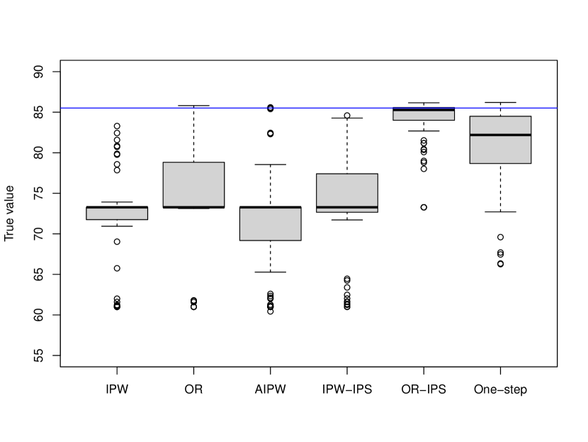
(a) Simulations.

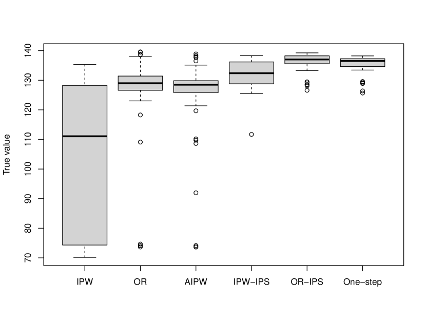
(b) Diabetes data application.

Figure 1: Performance of optimal policies under three standard methods (IPW, OR, AIPW) and our proposed three methods (IPW-IPS, OR-IPS, One-step). The blue line is the (approximate) true optimal value.

Additional simulation results are given in Section G of the Supplementary Material. Specifically, we illustrate that our proposed policy learning methods have comparable performance when there is no positivity violation, and also illustrate the better performance of our proposed methods when using parametric models.

6.2 Data application

We illustrate our proposed methods using semi-synthetic data from the Fairlearn open source project (Weerts et al., 2023). Additional information on our data analysis is provided in Section H of the Supplementary Material.

The Diabetes dataset represents ten years (1999-2008) of clinical care at 130 US hospitals and integrated delivery networks (Strack et al., 2014), and contains hospital records of patients diagnosed with diabetes who underwent laboratory tests and medications and stayed up to 14 days. Our application aims to learn the optimal policy for prescribing diabetic medication by maximizing the expected outcome under the demographic parity constraint. The sensitive attribute is race, and a violation of positivity exists in the data.

We include $7$ baseline covariates: race, gender, age, time_in_hospital (number of days between admission and discharge), num_lab_procedures (number of lab tests performed during the encounter), num_medications (number of distinct generic names administered during the encounter) and number_diagnoses (number of diagnoses). Under positivity violation, we are unable to identify the value function, e.g. relying on the outcome regression’s extrapolation to learn the counterfactual outcomes on test data. Thus the potential outcomes are simulated as follows: $Y(0)\sim\mathcal{N}\{20(1+{\tt gender}-{\tt age}+{\tt time\_in\_hospital}+{\tt num\_lab\_procedures}+{\tt num\_medications}+{\tt num\_medications}^{2}+\exp{({\tt number\_diagnoses})}),20^{2}\}$, and $Y(1)\sim\mathcal{N}\{20(1+{\tt gender}-{\tt age}+{\tt time\_in\_hospital}+{\tt num\_lab\_procedures}+{\tt num\_medications}+{\tt num\_medications}^{2}+\exp{({\tt number\_diagnoses})})+25(3-5{\tt age}+2{\tt time\_in\_hospital}-3{\tt num\_medications}+{\tt race}),20^{2}\}$. The estimation setup and policy classes are the same as previous simulations. We run $50$ repetitions; each time we randomly select $500$ patients as training data to learn the optimal policy and $2000$ patients as test data to evaluate the performance. Empirical results are reported in Figure 1(b). When the positivity violation is severer, the IPW estimator has extremely large variability, and we also observe that our proposed methods perform consistently better than the standard methods.

7 Discussion

This article proposes a general positivity-free stochastic policy learning framework using observational data, possibly subject to application-specific constraints. There are several interesting directions for future research. It is relevant to extend our methods to the more general case with multiple time points for treatment assignment, multiple treatment levels, or high-dimensional models (Wei et al., 2023), where positivity is even more likely to be violated. The incremental propensity score approach can also be extended to account for common issues such as covariate shift (Zhao et al., 2023; Lei et al., 2023), censoring and dropout (Cui et al., 2023), and truncation by death (Chu et al., 2023).

Acknowledgements

Pan Zhao and Julie Josse are supported in part by the French National Research Agency ANR-16-IDEX-0006. Shu Yang is partially supported by NSF SES 2242776, NIH 1R01AG066883 and 1R01ES031651, and FDA 1U01FD007934.

SUPPLEMENTARY MATERIAL

Appendix A Proof of Proposition 1

The proof of our identification results is straightforward, following similar arguments in Kennedy [2019]. First, we prove the OR-IPS formula:

$$V(d) =E[Y(d)]$$

$$=E[Y(1)d(X)+Y(0)(1-d(X))]$$

$$=E[E[Y(1)d(X)+Y(0)(1-d(X))\mid X]]$$

$$=E[d(X)E[Y(1)\mid X]+(1-d(X))E[Y(0)\mid X]]$$

$$=E[d(X)E[Y\mid X,A=1]+(1-d(X))E[Y\mid X,A=0]]$$

$$=E\left[\frac{\delta(X)\pi(X)}{\delta(X)\pi(X)+1-\pi(X)}\mu_{1}(X)+\frac{1-\pi(X)}{\delta(X)\pi(X)+1-\pi(X)}\mu_{0}(X)\right]$$

$$=E\left[\frac{\delta(X)\pi(X)\mu_{1}(X)+\{1-\pi(X)\}\mu_{0}(X)}{\delta(X)\pi(X)+1-\pi(X)}\right].$$

Next, we prove the IPW-IPS formula:

$$E\left[\frac{Y\{\delta(X)A+1-A\}}{\delta(X)\pi(X)+1-\pi(X)}\right]$$

$$=E\left[\frac{YA\delta(X)}{\delta(X)\pi(X)+1-\pi(X)}+\frac{Y(1-A)}{\delta(X)\pi(X)+1-\pi(X)}\right]$$

$$=E\left[\frac{Y(1)A\delta(X)}{\delta(X)\pi(X)+1-\pi(X)}+\frac{Y(0)(1-A)}{\delta(X)\pi(X)+1-\pi(X)}\right]$$

$$=E\left[E\left[\frac{Y(1)A\delta(X)}{\delta(X)\pi(X)+1-\pi(X)}+\frac{Y(0)(1-A)}{\delta(X)\pi(X)+1-\pi(X)}\mid X\right]\right]$$

$$=E\left[\frac{E[Y(1)A\mid X]\delta(X)}{\delta(X)\pi(X)+1-\pi(X)}+\frac{E[Y(0)(1-A)\mid X]}{\delta(X)\pi(X)+1-\pi(X)}\right]$$

$$=E\left[Y(1)\frac{E[A\mid X]\delta(X)}{\delta(X)\pi(X)+1-\pi(X)}+Y(0)\frac{E[(1-A)\mid X]}{\delta(X)\pi(X)+1-\pi(X)}\right]$$

$$=E[E[Y(1)d(X)+Y(0)(1-d(X))\mid X]]$$

$$=V(d).$$

Appendix B Proof of Proposition 2

We derive the efficient influence function for the following statistical functional:

$$\Psi(P)=E_{P}\left[\frac{\delta(X)\pi(X)\mu_{1}(X)+\{1-\pi(X)\}\mu_{0}(X)}{\delta(X)\pi(X)+1-\pi(X)}\right].$$

For a given distribution $P$ in the nonparametric statistical model $\mathcal{M}$, we let $p$ denote the density of $P$ with respect to some dominating measure $\nu$. For all bounded $h\in L_{2}(P)$, define the parametric submodel $p_{\epsilon}=(1+\epsilon h)p$, which is valid for small enough $\epsilon$ and has score $h$ at $\epsilon=0$. We would establish that $\Psi(P)$ is pathwise differentiable with respect to $\mathcal{M}$ at $P$ with efficient influence function $\phi(P)$ if we have that for any $P\in\mathcal{M}$,

$$\frac{\partial}{\partial\epsilon}\Psi(P_{\epsilon})\bigg{|}_{\epsilon=0}=\int\phi(P)(o)h(o)dP(o).$$

We denote $\pi_{\epsilon}(x)=E_{P_{\epsilon}}[A\mid X=x]$, $\mu_{a,\epsilon}(x)=E_{P_{\epsilon}}[Y\mid X=x,A=a]$, $S=\partial\log p_{\epsilon}/\partial\epsilon$, and can compute

$$\frac{\partial}{\partial\epsilon}\Psi(P_{\epsilon})\bigg{|}_{\epsilon=0} =\frac{\partial}{\partial\epsilon}E_{P_{\epsilon}}\left[\frac{\delta(X)\pi_{\epsilon}(X)\mu_{1,\epsilon}(X)+\{1-\pi_{\epsilon}(X)\}\mu_{0,\epsilon}(X)}{\delta(X)\pi_{\epsilon}(X)+1-\pi_{\epsilon}(X)}\right]\bigg{|}_{\epsilon=0}$$

$$=\frac{\partial}{\partial\epsilon}E_{P}\left[(1+\epsilon S)\frac{\delta(X)\pi_{\epsilon}(X)\mu_{1,\epsilon}(X)+\{1-\pi_{\epsilon}(X)\}\mu_{0,\epsilon}(X)}{\delta(X)\pi_{\epsilon}(X)+1-\pi_{\epsilon}(X)}\right]\bigg{|}_{\epsilon=0}$$

$$=E_{P}\left[S\frac{\delta(X)\pi(X)\mu_{1}(X)+\{1-\pi(X)\}\mu_{0}(X)}{\delta(X)\pi(X)+1-\pi(X)}\right]$$

$$\quad+E_{P}\left[\frac{1}{\delta(X)\pi(X)+1-\pi(X)}\left(\pi(X)\frac{\partial}{\partial\epsilon}\mu_{1,\epsilon}(X)\bigg{|}_{\epsilon=0}+\mu_{1}(X)\frac{\partial}{\partial\epsilon}\pi_{\epsilon}(X)\bigg{|}_{\epsilon=0}\right)\right]$$

$$\quad+E_{P}\left[\frac{1}{\delta(X)\pi(X)+1-\pi(X)}\left(\{1-\pi(X)\}\frac{\partial}{\partial\epsilon}\mu_{0,\epsilon}(X)\bigg{|}_{\epsilon=0}-\mu_{0}(X)\frac{\partial}{\partial\epsilon}\pi_{\epsilon}(X)\bigg{|}_{\epsilon=0}\right)\right]$$

$$\quad-E_{P}\left[\frac{\delta(X)\pi(X)\mu_{1}(X)+\{1-\pi(X)\}\mu_{0}(X)}{\{\delta(X)\pi(X)+1-\pi(X)\}^{2}}\left(\delta(X)\frac{\partial}{\partial\epsilon}\pi_{\epsilon}(X)\bigg{|}_{\epsilon=0}-\frac{\partial}{\partial\epsilon}\pi_{\epsilon}(X)\bigg{|}_{\epsilon=0}\right)\right].$$

Then we need to compute

$$\frac{\partial}{\partial\epsilon}\pi_{\epsilon}(X)\bigg{|}_{\epsilon=0} =\frac{\partial}{\partial\epsilon}\frac{\pi(X)+\epsilon E_{P}[SA\mid X]}{1+\epsilon E_{P}[S\mid X]}\bigg{|}_{\epsilon=0}$$

$$=E_{P}[SA\mid X]-\pi(X)E_{P}[S\mid X]$$

$$=E_{P}[S(A-\pi(X))\mid X],$$

and for $a=0,1$,

$$\frac{\partial}{\partial\epsilon}\mu_{a,\epsilon}(X)\bigg{|}_{\epsilon=0} =\frac{\partial}{\partial\epsilon}\frac{\mu_{a}(X)+\epsilon E_{P}[SY\mid X,A=a]}{1+\epsilon E_{P}[S\mid X,A=a]}\bigg{|}_{\epsilon=0}$$

$$=E_{P}[SY\mid X,A=a]-\mu_{a}(X)E_{P}[S\mid X,A=a]$$

$$=E_{P}[S(Y-\mu_{a}(X))\mid X,A=a].$$

Combining the above derivations, we obtain that

$$\phi(P)(O) =\frac{A\delta(X)\{Y-\mu_{1}(X)\}+(1-A)\{Y-\mu_{0}(X)\}+\delta(X)\pi(X)\mu_{1}(X)+\{1-\pi(X)\}\mu_{0}(X)}{\delta(X)\pi(X)+1-\pi(X)}$$

$$\quad+\frac{\delta(X)\tau(X)\{A-\pi(X)\}}{\{\delta(X)\pi(X)+1-\pi(X)\}^{2}}-\Psi(P),$$

which yields the result.

Appendix C Proof of Theorem 1

We first outline the inferential strategy from semiparametric theory. Consider a statistical model $\mathcal{M}$ for distributions $\tilde{P}$, with $P$ denoting the true distribution. Under sufficient smoothness conditions, we have the following von Mises expansion for $\Psi(\tilde{P})$:

$$\Psi(\tilde{P})=\Psi(P)-\int\phi(\tilde{P})(o)dP(o)+{\rm Rem}(\tilde{P},P),$$

where $\phi(P)$ is the influence function derived in Section B such that $\int\phi(P)(o)dP(o)=0$, and ${\rm Rem}(\tilde{P},P)=O(\|\tilde{P}-P\|^{2})$ is a second-order reminder term that we will analyze later.

Let $\hat{P}$ be an estimator of $P$, then we obtain the following one-step estimator of $\Psi(P)$:

$$\hat{\Psi}=\Psi(\hat{P})+\int\phi(\hat{P})(o)dP_{n}(o),$$

where $P_{n}$ is the empirical distribution.

Next, we characterize the asymptotic properties of $\hat{\Psi}$. Note that

$$\hat{\Psi}-\Psi(P) =\left\{\Psi(\hat{P})+\int\phi(\hat{P})(o)dP_{n}(o)\right\}-\Psi(P)$$

$$=\left\{\Psi(\hat{P})-\Psi(P)\right\}+\int\phi(\hat{P})(o)dP_{n}(o)$$

$$=-\int\phi(\hat{P})(o)dP(o)+{\rm Rem}(\hat{P},P)+\int\phi(\hat{P})(o)dP_{n}(o)$$

$$=\int\phi(\hat{P})(o)d\left\{P_{n}(o)-P(o)\right\}+{\rm Rem}(\hat{P},P)$$

$$=\int\phi(P)(o)dP_{n}(o)+\int\left\{\phi(\hat{P})(o)-\phi(P)(o)\right\}d\left\{P_{n}(o)-P(o)\right\}+{\rm Rem}(\hat{P},P).$$

Therefore, $\sqrt{n}\left\{\hat{\Psi}-\Psi(P)\right\}$ is expressed as the following three terms:

$$\sqrt{n}\left\{\hat{\Psi}-\Psi(P)\right\} =\sqrt{n}\int\phi(P)(o)dP_{n}(o)$$

$$\quad+\sqrt{n}\int\left\{\phi(\hat{P})(o)-\phi(P)(o)\right\}d\left\{P_{n}(o)-P(o)\right\}$$

$$\quad+\sqrt{n}{\rm Rem}(\hat{P},P).$$

By the central limit theorem, $\sqrt{n}\int\phi(P)(o)dP_{n}(o)$ is asymptotically normal with the asymptotic variance given by $E[\phi^{2}(P)(O)]$.

We assume that $\phi(P)$ belongs to a Donsker class, so we have that the centered empirical process

$$\sqrt{n}\int\left\{\phi(\hat{P})(o)-\phi(P)(o)\right\}d\left\{P_{n}(o)-P(o)\right\}=o_{p}(1).$$

Finally, we characterize the second-order remainder term:

$${\rm Rem}(\hat{P},P)=\Psi(\hat{P})-\Psi(P)+E_{P}[\phi(\hat{P})(O)].$$

We have that

$$\Psi(P)=E_{P}\left[\frac{\delta(X)\pi(X)\mu_{1}(X)+\{1-\pi(X)\}\mu_{0}(X)}{\delta(X)\pi(X)+1-\pi(X)}\right],$$

and

$$E_{P}[\phi(\hat{P})(O)]$$

$$=E_{P}\left[\frac{A\delta(X)\{Y-\hat{\mu}_{1}(X)\}+(1-A)\{Y-\hat{\mu}_{0}(X)\}+\delta(X)\hat{\pi}(X)\hat{\mu}_{1}(X)+\{1-\hat{\pi}(X)\}\hat{\mu}_{0}(X)}{\delta(X)\hat{\pi}(X)+1-\hat{\pi}(X)}\right.$$

$$\left.\qquad\quad+\frac{\delta(X)\hat{\tau}(X)\{A-\hat{\pi}(X)\}}{\{\delta(X)\hat{\pi}(X)+1-\hat{\pi}(X)\}^{2}}\right]-\Psi(\hat{P}).$$

Combining the derivations above, we have that

$$\left|{\rm Rem}(\hat{P},P)\right| \leq\hat{C}_{1}\|\hat{\mu}_{1}(X)-\mu_{1}(X)\|_{L_{2}}\times\|\hat{\pi}(X)-\pi(X)\|_{L_{2}}$$

$$\quad+\hat{C}_{2}\|\hat{\mu}_{0}(X)-\mu_{0}(X)\|_{L_{2}}\times\|\hat{\pi}(X)-\pi(X)\|_{L_{2}}$$

$$\quad+\hat{C}_{3}\|\hat{\pi}(X)-\pi(X)\|^{2}_{L_{2}},$$

where $\hat{C}_{1}$, $\hat{C}_{2}$ and $\hat{C}_{3}$ are $O_{p}(1)$. We assume that $\|\hat{\pi}(x)-\pi(x)\|_{L_{2}}=o_{p}(n^{-1/4})$, and $\|\hat{\mu}_{a}-\mu_{a}\|_{L_{2}}=o_{p}(n^{-1/4})$ for $a=0,1$. Therefore, we have that $\sqrt{n}{\rm Rem}(\hat{P},P)=o_{p}(1)$. That is, we conclude that

$$\sqrt{n}\left\{\hat{\Psi}-\Psi(P)\right\}\to\mathcal{N}(0,E[\phi^{2}(P)(O)]),$$

which completes the proof.

Appendix D Proof of Theorem 2

Essentially, we need to prove that the centered empirical process is $o_{p}(1)$, when we avoid Donsker conditions by using the cross-fitting technique. We first review a useful lemma from Kennedy et al. [2020].

Lemma 1.

Consider two independent samples $\mathcal{O}_{1}=(O_{1},\ldots,O_{n})$ and $\mathcal{O}_{2}=(O_{n+1},\ldots,O_{N})$ drawn from the distribution $\mathbb{P}$. Let $\hat{f}(o)$ be a function estimated from $\mathcal{O}_{2}$, and $\mathbb{P}_{n}$ the empirical measure over $\mathcal{O}_{1}$, then we have

$$(\mathbb{P}_{n}-\mathbb{P})(\hat{f}-f)=O_{\mathbb{P}}\left(\frac{\|\hat{f}-f\|}{\sqrt{n}}\right).$$

Proof.

First note that by conditioning on $\mathcal{O}_{2}$, we obtain that

$$\mathbb{E}\left\{\mathbb{P}_{n}(\hat{f}-f)\,\big{|}\,\mathcal{O}_{2}\right\}=\mathbb{E}(\hat{f}-f\,|\,\mathcal{O}_{2})=\mathbb{P}(\hat{f}-f),$$

and the conditional variance is

$$var\{(\mathbb{P}_{n}-\mathbb{P})(\hat{f}-f)\,|\,\mathcal{O}_{2}\}=var\{\mathbb{P}_{n}(\hat{f}-f)\,|\,\mathcal{O}_{2}\}=\frac{1}{n}var(\hat{f}-f\,|\,\mathcal{O}_{2})\leq\|\hat{f}-f\|^{2}/n,$$

therefore by the Chebyshev’s inequality we have that

$$\mathbb{P}\left\{\frac{|(\mathbb{P}_{n}-\mathbb{P})(\hat{f}-f)|}{\|\hat{f}-f\|^{2}/n}\geq t\right\}=\mathbb{E}\left[\mathbb{P}\left\{\frac{|(\mathbb{P}_{n}-\mathbb{P})(\hat{f}-f)|}{\|\hat{f}-f\|^{2}/n}\geq t\,\bigg{|}\,\mathcal{O}_{2}\right\}\right]\leq\frac{1}{t^{2}},$$

thus for any $\epsilon>0$ we can pick $t=1/\sqrt{\epsilon}$ so that the probability above is no more than $\epsilon$, which yields the result. ∎

Next, we characterize the asymptotic properties of the cross-fitted estimator $\hat{\Psi}_{\rm CF}$. Following similar steps as Section C, we have that

$$\sqrt{n}\left\{\hat{\Psi}_{\rm CF}-\Psi(P)\right\}=\sqrt{n}\int\phi(P)(o)dP_{n}(o)+\frac{1}{\sqrt{K}}\sum_{k=1}^{K}\sqrt{n_{k}}(R_{k,1}+R_{k,2}),$$

where $R_{k,1}=\int\left\{\phi(\hat{P}_{-k})(o)-\phi(P)(o)\right\}d\left\{P_{n,k}(o)-P(o)\right\}$, $R_{k,2}={\rm Rem}(\hat{P}_{-k},P)$.

We note that

$$R_{k,1} =\int\left\{\phi(\hat{P}_{-k})(o)-\phi(P)(o)\right\}d\left\{P_{n,k}(o)-P(o)\right\}$$

$$=\int\left\{\xi(\hat{P}_{-k})(o)-\xi(P)(o)\right\}d\left\{P_{n,k}(o)-P(o)\right\},$$

where $\xi(P)(o)=\phi(P)(o)+\Psi(P)$, and by Lemma 1, we have that

$$\sqrt{n_{k}}R_{k,1}=O_{p}\left(\|\xi(\hat{P}_{-k})-\xi(P)\|_{L_{2}}\right).$$

Note that

$$\xi(\hat{P}_{-k})(O)-\xi(P)(O)$$

$$=\frac{A\delta(X)\{Y-\mu_{1}(X)\}+(1-A)\{Y-\mu_{0}(X)\}}{\delta(X)\pi(X)+1-\pi(X)}-\frac{A\delta(X)\{Y-\mu_{1}(X)\}+(1-A)\{Y-\mu_{0}(X)\}}{\delta(X)\pi(X)+1-\pi(X)}$$

$$\quad+\frac{\delta(X)\pi(X)\mu_{1}(X)+\{1-\pi(X)\}\mu_{0}(X)}{\delta(X)\pi(X)+1-\pi(X)}-\frac{\delta(X)\pi(X)\mu_{1}(X)+\{1-\pi(X)\}\mu_{0}(X)}{\delta(X)\pi(X)+1-\pi(X)}$$

$$\quad+\frac{\delta(X)\tau(X)\{A-\pi(X)\}}{\{\delta(X)\pi(X)+1-\pi(X)\}^{2}}-\frac{\delta(X)\tau(X)\{A-\pi(X)\}}{\{\delta(X)\pi(X)+1-\pi(X)\}^{2}},$$

and we assume that $|Y|$ and $|\delta(X)|$ are bounded in probability. By the triangle and Cauchy-Schwarz inequalities, we have that

$$\|\xi(\hat{P}_{-k})-\xi(P)\|_{L_{2}} \leq\hat{C}_{1,-k}\|\hat{\mu}_{0,-k}(X)-\mu_{0}(X)\|_{L_{2}}+\hat{C}_{2,-k}\|\hat{\mu}_{1,-k}(X)-\mu_{1}(X)\|_{L_{2}}$$

$$\qquad+\hat{C}_{3,-k}\|\hat{\pi}_{-k}(X)-\pi(X)\|_{L_{2}}$$

where $\hat{C}_{1,-k}$, $\hat{C}_{2,-k}$ and $\hat{C}_{3,-k}$ are $O_{p}(1)$. We assume that $\|\hat{\pi}(x)-\pi(x)\|_{L_{2}}=o_{p}(n^{-1/4})$, and $\|\hat{\mu}_{a}-\mu_{a}\|_{L_{2}}=o_{p}(n^{-1/4})$ for $a=0,1$. Therefore, we have that $\sqrt{n_{k}}R_{k,1}=o_{p}(1)$.

By the same arguments as Section C, we have that $\sqrt{n_{k}}R_{k,2}=o_{p}(1)$. That is, we conclude that

$$\sqrt{n}\left\{\hat{\Psi}_{\rm CF}-\Psi(P)\right\}\to\mathcal{N}(0,E[\phi^{2}(P)(O)]),$$

which completes the proof.

Appendix E Proof of Theorem 3

In this section, we consider a parametric policy class $\mathcal{D}(H)$ indexed by $\eta\in H$. That is, the off-policy learning task is given by the following optimization problem:

$$\eta^{\ast}=\arg\max_{\eta\in H} \quad V(\eta),$$

subject to $$\quad c(\eta)\leq 0,$$

and the estimated policy is given by

$$\hat{\eta}=\arg\max_{\eta\in H} \quad\hat{V}(\eta),$$

subject to $$\quad\hat{c}(\eta)\leq 0.$$

We first review a useful lemma from Shapiro [1991].

Lemma 2.

Let $H$ be a compact subset of $\mathbb{R}^{k}$. Let $C(H)$ denote the set of continuous real-valued functions on $H$, with $\mathcal{L}=C(H)\times\cdots\times C(H)$ the $r$-dimensional Cartesian product. Let $f(\eta)=(f_{0},\ldots,f_{r})\in\mathcal{L}$ be a vector of convex functions. Consider the quantity $\eta^{\ast}$ defined as the solution to the following convex optimization program:

$$\eta^{\ast}= \arg\min_{\eta\in H}f_{0}(\eta),$$

subject to $$f_{j}(\eta)\leq 0,j=1,\ldots,r.$$

Assume that Slater’s condition holds, so that there is some $\eta\in H$ for which the inequalities are satisfied and non-affine inequalities are strictly satisfied, i.e. $f_{j}(\eta)<0$ if $f_{j}(\eta)$ is non-affine. Now consider a sequence of approximating programs, for $n=1,2,\ldots$:

$$\hat{\eta}_{n}= \arg\min_{\eta\in H}\hat{f}_{n,0}(\eta),$$

subject to $$\hat{f}_{n,j}(\eta)\leq 0,j=1,\ldots,r,$$

with $\hat{f}_{n}(\eta)=\left(\hat{f}_{n,0},\ldots,\hat{f}_{n,r}\right)\in\mathcal{L}$. Assume that $r(n)\left(\hat{f}_{n}-f\right)$ converges in distribution to a random element $W\in\mathcal{L}$ for some real-valued function $f(\eta)$. Then

$$r(n)\left(\hat{f}_{n,0}(\eta)(\hat{\eta}_{n})-f_{0}(\eta^{\ast})\right)\to L,$$

for a particular random variable $L$. It follows that $\hat{f}_{n,0}(\eta)(\hat{\eta}_{n})-f_{0}(\eta^{\ast})=O_{p}(1/r(n))$.

By Theorem 1 or 2, we have that

$$\sqrt{n}\left(\hat{V}(\eta)-V(\eta)\right)=\frac{1}{\sqrt{n}}\sum_{i=1}^{n}\phi_{V}(O_{i};\eta)+o_{p}(1),$$

and by condition (ii), we have that

$$\sqrt{n}\left(\hat{c}(\eta)-c(\eta)\right)=\frac{1}{\sqrt{n}}\sum_{i=1}^{n}\phi_{c}(O_{i};\eta)+o_{p}(1),$$

where $\phi_{V}$ and $\phi_{c}$ are the influence functions.

By condition (i) and Lemma 2 with $r(n)=\sqrt{n}$, we obtain the conclusion (ii).

To prove conclusion (i), note that

$$V(\hat{\eta})-V(\eta^{\ast})=V(\hat{\eta})-\hat{V}(\hat{\eta})+\hat{V}(\hat{\eta})-V(\eta^{\ast}),$$

where we have that $V(\hat{\eta})-\hat{V}(\hat{\eta})=O_{p}(n^{-1/2})$, and $\hat{V}(\hat{\eta})-V(\eta^{\ast})=O_{p}(n^{-1/2})$. Hence, we conclude that $V(\hat{\eta})-V(\eta^{\ast})=O_{p}(n^{-1/2})$, which completes the proof.

Appendix F Proof of Theorem 4

In this section, we follow similar techniques in Li et al. [2023] and consider the off-policy learning task given by the following optimization problem:

$$d^{\ast}=\arg\max_{d\in\mathcal{D}} \,V(d)=\arg\max_{d\in\mathcal{D}}E[\xi(P)(O)],$$

subject to $$\,c(d)=E[\phi_{c}(P)(O)]\leq 0,$$

where $\mathcal{D}$ is a Glivenko–Cantelli class, and the estimated optimal policy is given by

$$\hat{d}=\arg\max_{d\in\mathcal{D}} \,\hat{V}(d)=\arg\max_{d\in\mathcal{D}}\frac{1}{n}\sum_{i=1}^{n}\xi(\hat{P})(O_{i})$$

subject to $$\,\hat{c}(d)=\frac{1}{n}\sum_{i=1}^{n}\phi_{c}(\hat{P})(O_{i})\leq 0.$$

By condition (iii) of Theorems 1 or condition (ii) of Theorems 2, we have that both $\{\xi(O;d):d\in\mathcal{D}\}$ and $\{\phi_{c}(O;d):d\in\mathcal{D}\}$ are GC classes.

To simplify the notation, let we denote $\mathcal{D}_{c}=\left\{d\in\mathcal{D}:c(d)\leq 0\right\}$, and $\mathcal{D}_{n,c}=\left\{d\in\mathcal{D}:\hat{c}(d)\leq 0\right\}$. First we note that the estimation error can be expressed as

$$V(d^{\ast})-\hat{V}(\hat{d})=V_{n}^{(1)}+V_{n}^{(2)}+V_{n}^{(3)},$$

where we define

$$V_{n}^{(1)} =\max_{d\in\mathcal{D}_{c}}E[\xi(P)(O)]-\max_{d\in\mathcal{D}_{c}}P_{n}\xi(P)(O),$$

$$V_{n}^{(2)} =\max_{d\in\mathcal{D}_{c}}P_{n}\xi(P)(O)-\max_{d\in\mathcal{D}_{c}}P_{n}\xi(\hat{P})(O),$$

$$V_{n}^{(3)} =\max_{d\in\mathcal{D}_{c}}P_{n}\xi(\hat{P})(O)-\max_{d\in\mathcal{D}_{n,c}}P_{n}\xi(\hat{P})(O).$$

We analyze the three terms as follows. We have that

$$V_{n}^{(1)} =\max_{d\in\mathcal{D}_{c}}E[\xi(P)(O)]-\max_{d\in\mathcal{D}_{c}}P_{n}\xi(P)(O)$$

$$\leq\max_{d\in\mathcal{D}_{c}}\left|E[\xi(P)(O)]-P_{n}\xi(P)(O)\right|$$

$$=o_{p}(1),$$

and similarly we have that

$$V_{n}^{(2)} =\max_{d\in\mathcal{D}_{c}}P_{n}\xi(P)(O)-\max_{d\in\mathcal{D}_{c}}P_{n}\xi(\hat{P})(O)$$

$$\leq\max_{d\in\mathcal{D}_{c}}\left|P_{n}\{\xi(P)(O)-\xi(\hat{P})(O)\}\right|$$

$$=o_{p}(1).$$

To analyze $V_{n}^{(3)}$, note that for any $d\in\mathcal{D}$, we have that

$$E[\phi_{c}(P)(O)]-P_{n}\phi_{c}(\hat{P})(O)$$

$$=\{E[\phi_{c}(P)(O)]-P_{n}\phi_{c}(P)(O)\}+\{P_{n}\phi_{c}(P)(O)-P_{n}\phi_{c}(\hat{P})(O)\},$$

and $E[\phi_{c}(P)(O)]-P_{n}\phi_{c}(P)(O)$ converges to $0$ uniformly as $\{\phi_{c}(O;d):d\in\mathcal{D}\}$ is a GC class, and $P_{n}\phi_{c}(P)(O)-P_{n}\phi_{c}(\hat{P})(O)$ converges to $0$ uniformly by condition (ii).

Hence, $\forall\epsilon>0$, $\exists N_{1}\in\mathbb{N}$, such that for all $n>N_{1}$, $|E[\phi_{c}(P)(O)]-P_{n}\phi_{c}(\hat{P})(O)|<\epsilon$, by which we obtain that, for all $d\in\mathcal{D}_{c}$, i.e., $E[\phi_{c}(P)(O)]\leq c$, we have that $P_{n}\phi_{c}(\hat{P})(O)<c+\epsilon$. Therefore, we have that $\frac{c}{c+\epsilon}d\in\mathcal{D}_{n,c}$.

As $\xi(\hat{P})(O)$ is uniformly bounded, there exists a constant $L>0$ such that for any $d_{1},d_{2}$, we have that

$$|\xi(\hat{P})(O;d_{1})-\xi(\hat{P})(O;d_{2})|\leq L\sup_{x\in\mathcal{X}}|d_{1}(x)-d_{2}(x)|.$$

Thus, $\forall\epsilon>0$, $\exists N_{1}\in\mathbb{N}$, such that for all $n>N_{1}$,

$$V_{n}^{(3)} =\max_{d\in\mathcal{D}_{c}}P_{n}\xi(\hat{P})(O)-\max_{d\in\mathcal{D}_{n,c}}P_{n}\xi(\hat{P})(O)$$

$$\leq\max_{d\in\mathcal{D}_{c}}P_{n}\xi(\hat{P})(O)-\max_{d\in\frac{c}{c+\epsilon}\mathcal{D}_{c}}P_{n}\xi(\hat{P})(O)$$

$$\leq\frac{\epsilon}{c+\epsilon}L,$$

and similarly, we can obtain that $\exists N_{2}\in\mathbb{N}$, such that for all $n>N_{2}$,

$$V_{n}^{(3)}\geq-\frac{\epsilon}{c+\epsilon}L,$$

which in combination implies that $V_{n}^{(3)}=o_{p}(1)$.

Next, we prove our result (ii) for the regret. Note that

$$V(d^{\ast})-V(\hat{d})=\{V(d^{\ast})-\hat{V}(d^{\ast})\}+\{\hat{V}(d^{\ast})-\hat{V}(\hat{d})\}+\{\hat{V}(\hat{d})-V(\hat{d})\}.$$

We analyze the three terms as follows. By the same argument for proving (i), we have that

$$V(d^{\ast})-\hat{V}(d^{\ast}) =E[\xi(P)(O;d^{\ast})]-P_{n}\xi(\hat{P})(O;d^{\ast})=o_{p}(1),$$

$$\hat{V}(\hat{d})-V(\hat{d}) =P_{n}\xi(\hat{P})(O;\hat{d})-E[\xi(P)(O;\hat{d})]=o_{p}(1).$$

Also by a similar argument, we have that for any $d\in\mathcal{D}$ and $\epsilon>0$, $\exists N_{2}\in\mathbb{N}$, for all $n>N_{2}$, $\frac{c}{c+\epsilon}d\in\mathcal{D}_{n,c}$, and

$$\hat{V}(d^{\ast})-\hat{V}(\hat{d}) =\hat{V}(d^{\ast})-\hat{V}\left(\frac{c}{c+\epsilon}d^{\ast}\right)+\hat{V}\left(\frac{c}{c+\epsilon}d^{\ast}\right)-\hat{V}(\hat{d})$$

$$\leq\frac{\epsilon}{c+\epsilon}L,$$

and also that for any $d\in\mathcal{D}$ and $\epsilon>0$, $\exists N_{3}\in\mathbb{N}$, for all $n>N_{3}$, $\frac{c}{c+\epsilon}\hat{d}\in\mathcal{D}_{n,c}$, and

$$V(d^{\ast})-V(\hat{d})\geq V\left(\frac{c}{c+\epsilon}\hat{d}\right)-V(\hat{d})\geq-\frac{\epsilon}{c}L,$$

so we conclude that $V(d^{\ast})-V(\hat{d})=o_{p}(1)$, which completes the proof.

Appendix G Additional simulations

In this section, we present additional simulation results.

G.1 Incremental propensity score policy learning with sufficent overlap

We examine the performance of our proposed methods by comparison with standard policy learning methods, when sufficient overlap indeed holds. We consider the following data generating process:

$$(X_{1},X_{2}) \sim\text{Uniform}(0,1),$$

$$(X_{3},X_{4}) \sim\mathcal{N}\left\{\left(\begin{smallmatrix}0\\ 0\end{smallmatrix}\right),\left(\begin{smallmatrix}1&0.3\\ 0.3&1\end{smallmatrix}\right)\right\},$$

$$A \sim\text{Bernoulli}(\text{expit}(0.3-0.4X_{1}-0.2X_{2}-0.3X_{3}+0.1X_{4})),$$

$$Y(0) \sim\mathcal{N}\{20(1+X_{1}-X_{2}+X_{3}^{2}+\exp{(X_{2})}),20^{2}\},$$

$$Y(1) \sim\mathcal{N}\{20(1+X_{1}-X_{2}+X_{3}^{2}+\exp{(X_{2})})+25(3-5X_{1}+2X_{2}-3X_{3}+X_{4}),20^{2}\}.$$

We perform the vanilla direct policy search tasks without constraint. Hence, the optimal policy is simply $d^{\ast}(x)=I\{3-5X_{1}+2X_{2}-3X_{3}+X_{4}>0\}$. For standard methods, we consider the policy class of linear rules $\mathcal{D}_{\rm linear}=\{d(x)=I\{(1,x_{1},x_{2},x_{3},x_{4})\beta>0\}:\beta\in\mathbb{R}^{5},\|\beta\|_{2}=1\}$. For the incremental propensity score policies, we consider the class $\mathcal{D}_{\rm IPS}=\{d(x)=\delta(x;\beta)\pi(x)/\{\delta(x;\beta)\pi(x)+1-\pi(x)\}:\beta\in\mathbb{R}^{5}\}$, which is indexed by $\delta(x;\beta)=\exp{\{(1,x_{1},x_{2},x_{3},x_{4})\beta\}}$.

We estimate the outcome regression model $\mu(x)$ and the propensity score $\pi(x)$ using the generalized random forests [Athey et al., 2019] implemented in the R package grf. The unconstrained optimization problems are solved by the genetic algorithm [Sekhon and Mebane, 1998] implemented in the R package rgenoud. The sample size is $n=2000$. We compare the true values of the estimated optimal policies using test data with sample size $N=10^{5}$. The true optimal value is approximated using the test data. Simulation results of $100$ Monte Carlo repetition are reported in Figure 2(a).

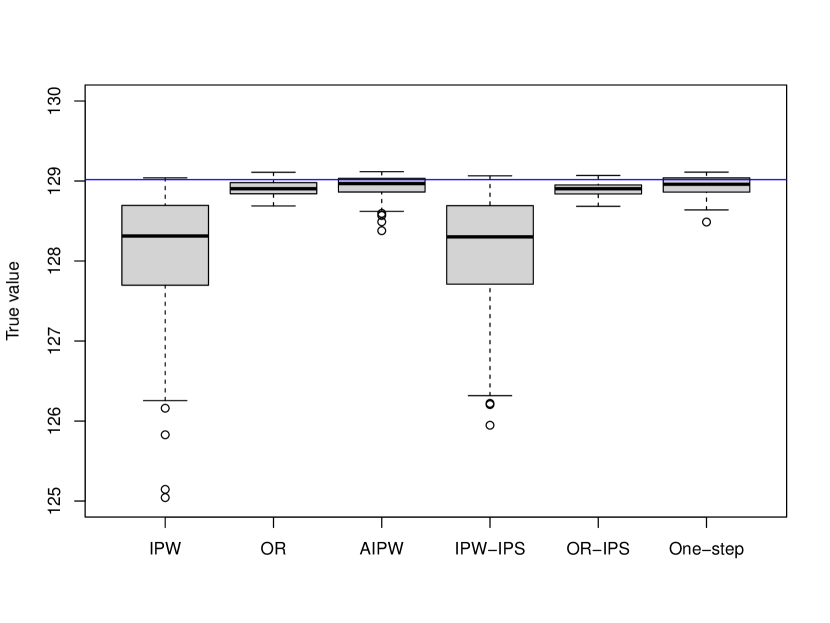
(a) Sufficient overlap.

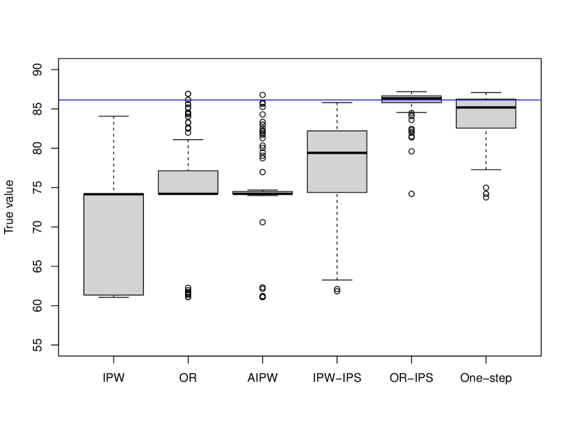
(b) Parametric models.

Figure 2: Performance of optimal policies under three standard methods (IPW, OR, AIPW) and our proposed three methods (IPW-IPS, OR-IPS, One-step). The blue line is the (approximate) true optimal value.

Despite the fact that the true optimal rule is included in the standard policy class of linear rules but not in our proposed class of incremental propensity score policies, we still observe comparable performance of both classes, which exemplifies the effectiveness of our proposed methods.

G.2 Incremental propensity score policy learning with parametric models

We examine the performance of our proposed methods by comparison with standard policy learning methods, when using correctly specified parametric models.

The simulation setup is the same as in the main paper where the positivity assumption is violated, except that the sample size $n=500$ is smaller and the outcome regression $\mu(s,x)$ and the propensity score $\pi(s,x)$ models are estimated by correctly specified parametric models. Simulation results of $100$ Monte Carlo repetition are reported in Figure 2(b). The standard methods IPW, OR, and AIPW have the worst performance. The IPW-IPS estimator still has large variability, and the OR-IPS and efficient one-step estimators achieve the best performance with the highest value.

Appendix H Diabetes data analysis

In this section, we provide supplementary information on our Diabetes data analysis.

The original dataset is available in the UCI Repository Diabetes 130-US hospitals for years 1999-2008 [Strack et al., 2014]. The Fairlearn open source project [Weerts et al., 2023] provides full dataset pre-processing script in python on GitHub. We follow these pre-processing steps, and provide the R script.

The dataset contains $101766$ patients, and a detailed description of the $25$ variables are available at the Fairlearn project. Originally, the categories of race include “African American”, “Asian”, “Caucasian”, “Hispanic”, “Other”, “Unknown”, and the categories of age include “$30$ years or younger”, “$30-60$ years”, “Over $60$ years”. We dichotomize them, so the resultant categories of race include “Caucasian” or “Non-Caucasian”, and the resultant categories of age include “$30$ years or younger” or “Over $30$ years”.

The missing data are completed by multivariate imputation by chained equations, implemented in the R package mice.

References

- Athey and Wager [2021] Susan Athey and Stefan Wager. Policy learning with observational data. Econometrica, 89(1):133–161, 2021.
- Athey et al. [2019] Susan Athey, Julie Tibshirani, and Stefan Wager. Generalized random forests. The Annals of Statistics, 47(2):1148 – 1178, 2019. doi: 10.1214/18-AOS1709. URL https://doi.org/10.1214/18-AOS1709.
- Bibaut et al. [2021] Aurélien Bibaut, Nathan Kallus, Maria Dimakopoulou, Antoine Chambaz, and Mark van Der Laan. Risk minimization from adaptively collected data: Guarantees for supervised and policy learning. Advances in neural information processing systems, 34:19261–19273, 2021.
- Bickel et al. [1993] Peter J Bickel, Chris AJ Klaassen, Peter J Bickel, Ya’acov Ritov, J Klaassen, Jon A Wellner, and YA’Acov Ritov. Efficient and adaptive estimation for semiparametric models, volume 4. Springer, 1993.
- Branson et al. [2023] Zach Branson, Edward H Kennedy, Sivaraman Balakrishnan, and Larry Wasserman. Causal effect estimation after propensity score trimming with continuous treatments. arXiv preprint arXiv:2309.00706, 2023.
- Calders et al. [2009] Toon Calders, Faisal Kamiran, and Mykola Pechenizkiy. Building classifiers with independency constraints. In 2009 IEEE international conference on data mining workshops, pages 13–18. IEEE, 2009.
- Chernozhukov et al. [2018] Victor Chernozhukov, Denis Chetverikov, Mert Demirer, Esther Duflo, Christian Hansen, Whitney Newey, and James Robins. Double/debiased machine learning for treatment and structural parameters. The Econometrics Journal, 21(1):C1–C68, 01 2018. ISSN 1368-4221.
- Chu et al. [2023] Jianing Chu, Shu Yang, and Wenbin Lu. Multiply robust off-policy evaluation and learning under truncation by death. In Andreas Krause, Emma Brunskill, Kyunghyun Cho, Barbara Engelhardt, Sivan Sabato, and Jonathan Scarlett, editors, Proceedings of the 40th International Conference on Machine Learning, volume 202 of Proceedings of Machine Learning Research, pages 6195–6227. PMLR, 23–29 Jul 2023.
- Chzhen et al. [2020] Evgenii Chzhen, Christophe Denis, Mohamed Hebiri, Luca Oneto, and Massimiliano Pontil. Fair regression with wasserstein barycenters. In H. Larochelle, M. Ranzato, R. Hadsell, M.F. Balcan, and H. Lin, editors, Advances in Neural Information Processing Systems, volume 33, pages 7321–7331. Curran Associates, Inc., 2020.
- Cortez et al. [2022] Mayleen Cortez, Matthew Eichhorn, and Christina Yu. Staggered rollout designs enable causal inference under interference without network knowledge. In S. Koyejo, S. Mohamed, A. Agarwal, D. Belgrave, K. Cho, and A. Oh, editors, Advances in Neural Information Processing Systems, volume 35, pages 7437–7449. Curran Associates, Inc., 2022.
- Cui et al. [2017] Yifan Cui, Ruoqing Zhu, and Michael Kosorok. Tree based weighted learning for estimating individualized treatment rules with censored data. Electronic journal of statistics, 11(2):3927, 2017.
- Cui et al. [2023] Yifan Cui, Michael R Kosorok, Erik Sverdrup, Stefan Wager, and Ruoqing Zhu. Estimating heterogeneous treatment effects with right-censored data via causal survival forests. Journal of the Royal Statistical Society Series B: Statistical Methodology, 85(2):179–211, 2023.
- Dudík et al. [2014] Miroslav Dudík, Dumitru Erhan, John Langford, and Lihong Li. Doubly robust policy evaluation and optimization. Statistical Science, 29:485–511, 2014.
- Fang et al. [2022] Ethan X Fang, Zhaoran Wang, and Lan Wang. Fairness-oriented learning for optimal individualized treatment rules. Journal of the American Statistical Association, pages 1–14, 2022.
- Foster and Syrgkanis [2023] Dylan J Foster and Vasilis Syrgkanis. Orthogonal statistical learning. The Annals of Statistics, 51(3):879–908, 2023.
- Gui and Veitch [2023] Lin Gui and Victor Veitch. Causal estimation for text data with (apparent) overlap violations. In International Conference on Learning Representations, 2023.
- Haneuse and Rotnitzky [2013] Sebastian Haneuse and Andrea Rotnitzky. Estimation of the effect of interventions that modify the received treatment. Statistics in medicine, 32(30):5260–5277, 2013.
- Hardt et al. [2016] Moritz Hardt, Eric Price, and Nati Srebro. Equality of opportunity in supervised learning. Advances in neural information processing systems, 29, 2016.
- Imbens and Rubin [2015] Guido W Imbens and Donald B Rubin. Causal inference in statistics, social, and biomedical sciences. Cambridge University Press, 2015.
- Jia et al. [2023] Zeyang Jia, Eli Ben-Michael, and Kosuke Imai. Bayesian safe policy learning with chance constrained optimization: Application to military security assessment during the vietnam war. arXiv preprint arXiv:2307.08840, 2023.
- Jin et al. [2022] Ying Jin, Zhimei Ren, Zhuoran Yang, and Zhaoran Wang. Policy learning “without” overlap: Pessimism and generalized empirical bernstein’s inequality. arXiv preprint arXiv:2212.09900, 2022.
- Kallus and Oprescu [2023] Nathan Kallus and Miruna Oprescu. Robust and agnostic learning of conditional distributional treatment effects. In International Conference on Artificial Intelligence and Statistics, pages 6037–6060. PMLR, 2023.
- Kallus and Uehara [2020] Nathan Kallus and Masatoshi Uehara. Efficient evaluation of natural stochastic policies in offline reinforcement learning. arXiv preprint arXiv:2006.03886, 2020.
- Kallus and Zhou [2018] Nathan Kallus and Angela Zhou. Confounding-robust policy improvement. Advances in neural information processing systems, 31, 2018.
- Kennedy [2019] Edward H Kennedy. Nonparametric causal effects based on incremental propensity score interventions. Journal of the American Statistical Association, 114(526):645–656, 2019.
- Kennedy [2022] Edward H Kennedy. Semiparametric doubly robust targeted double machine learning: a review. arXiv preprint arXiv:2203.06469, 2022.
- Kennedy et al. [2020] Edward H. Kennedy, Sivaraman Balakrishnan, and Max G’Sell. Sharp instruments for classifying compliers and generalizing causal effects. The Annals of Statistics, 48(4):2008 – 2030, 2020.
- Khan et al. [2023] Samir Khan, Martin Saveski, and Johan Ugander. Off-policy evaluation beyond overlap: partial identification through smoothness. arXiv preprint arXiv:2305.11812, 2023.
- Künzel et al. [2019] Sören R Künzel, Jasjeet S Sekhon, Peter J Bickel, and Bin Yu. Metalearners for estimating heterogeneous treatment effects using machine learning. Proceedings of the national academy of sciences, 116(10):4156–4165, 2019.
- Lawrence et al. [2017] Carolin Lawrence, Artem Sokolov, and Stefan Riezler. Counterfactual learning from bandit feedback under deterministic logging: A case study in statistical machine translation. arXiv preprint arXiv:1707.09118, 2017.
- Lei et al. [2023] Lihua Lei, Roshni Sahoo, and Stefan Wager. Policy learning under biased sample selection. arXiv preprint arXiv:2304.11735, 2023.
- Li et al. [2023] Haoxuan Li, Chunyuan Zheng, Yixiao Cao, Zhi Geng, Yue Liu, and Peng Wu. Trustworthy policy learning under the counterfactual no-harm criterion. In Andreas Krause, Emma Brunskill, Kyunghyun Cho, Barbara Engelhardt, Sivan Sabato, and Jonathan Scarlett, editors, Proceedings of the 40th International Conference on Machine Learning, volume 202 of Proceedings of Machine Learning Research, pages 20575–20598. PMLR, 23–29 Jul 2023.
- Liu et al. [2023] Yi Liu, Huiyue Li, Yunji Zhou, and Roland Matsouaka. Average treatment effect on the treated, under lack of positivity. arXiv preprint arXiv:2309.01334, 2023.
- Luedtke and van der Laan [2016a] Alexander R Luedtke and Mark J van der Laan. Optimal individualized treatments in resource-limited settings. The international journal of biostatistics, 12(1):283–303, 2016a.
- Luedtke and van der Laan [2016b] Alexander R Luedtke and Mark J van der Laan. Statistical inference for the mean outcome under a possibly non-unique optimal treatment strategy. Annals of statistics, 44(2):713, 2016b.
- Muñoz and van Der Laan [2012] Iván Díaz Muñoz and Mark van Der Laan. Population intervention causal effects based on stochastic interventions. Biometrics, 68(2):541–549, 2012.
- Murphy [2003] Susan A Murphy. Optimal dynamic treatment regimes. Journal of the Royal Statistical Society Series B: Statistical Methodology, 65(2):331–355, 2003.
- Murphy et al. [2001] Susan A Murphy, Mark J van der Laan, James M Robins, and Conduct Problems Prevention Research Group. Marginal mean models for dynamic regimes. Journal of the American Statistical Association, 96(456):1410–1423, 2001.
- Neyman [1923] Jersey Neyman. Sur les applications de la théorie des probabilités aux experiences agricoles: Essai des principes. Roczniki Nauk Rolniczych, 10(1):1–51, 1923.
- Nie and Wager [2021] Xinkun Nie and Stefan Wager. Quasi-oracle estimation of heterogeneous treatment effects. Biometrika, 108(2):299–319, 2021.
- Powell [1994] Michael JD Powell. A direct search optimization method that models the objective and constraint functions by linear interpolation. Springer, 1994.
- Qiu et al. [2021] Hongxiang Qiu, Marco Carone, Ekaterina Sadikova, Maria Petukhova, Ronald C Kessler, and Alex Luedtke. Optimal individualized decision rules using instrumental variable methods. Journal of the American Statistical Association, 116(533):174–191, 2021.
- Rubin [1974] Donald B Rubin. Estimating causal effects of treatments in randomized and nonrandomized studies. Journal of educational Psychology, 66(5):688, 1974.
- Sekhon and Mebane [1998] Jasjeet S Sekhon and Walter R Mebane. Genetic optimization using derivatives. Political Analysis, 7:187–210, 1998.
- Shapiro [1991] Alexander Shapiro. Asymptotic analysis of stochastic programs. Annals of Operations Research, 30:169–186, 1991.
- Shi et al. [2018] Chengchun Shi, Ailin Fan, Rui Song, and Wenbin Lu. High-dimensional -learning for optimal dynamic treatment regimes. The Annals of Statistics, 46(3):925 – 957, 2018.
- Strack et al. [2014] Beata Strack, Jonathan P DeShazo, Chris Gennings, Juan L Olmo, Sebastian Ventura, Krzysztof J Cios, John N Clore, et al. Impact of hba1c measurement on hospital readmission rates: analysis of 70,000 clinical database patient records. BioMed research international, 2014, 2014.
- Tian [2008] Jin Tian. Identifying dynamic sequential plans. In Proceedings of the Twenty-Fourth Conference on Uncertainty in Artificial Intelligence, 2008.
- Tsiatis et al. [2019] Anastasios A Tsiatis, Marie Davidian, Shannon T Holloway, and Eric B Laber. Dynamic treatment regimes: Statistical methods for precision medicine. CRC press, 2019.
- Uehara et al. [2022] Masatoshi Uehara, Chengchun Shi, and Nathan Kallus. A review of off-policy evaluation in reinforcement learning. arXiv preprint arXiv:2212.06355, 2022.
- van der Laan and Petersen [2007] Mark J van der Laan and Maya L Petersen. Causal effect models for realistic individualized treatment and intention to treat rules. The international journal of biostatistics, 3(1), 2007.
- van der Laan and Robins [2003] Mark J van der Laan and James M Robins. Unified methods for censored longitudinal data and causality. Springer, 2003.
- van der Laan et al. [2011] Mark J van der Laan, Sherri Rose, et al. Targeted learning: causal inference for observational and experimental data, volume 4. Springer, 2011.
- Wager and Athey [2018] Stefan Wager and Susan Athey. Estimation and inference of heterogeneous treatment effects using random forests. Journal of the American Statistical Association, 113(523):1228–1242, 2018.
- Weerts et al. [2023] Hilde Weerts, Miroslav Dudík, Richard Edgar, Adrin Jalali, Roman Lutz, and Michael Madaio. Fairlearn: Assessing and improving fairness of ai systems. Journal of Machine Learning Research, 24(257):1–8, 2023.
- Wei et al. [2023] Waverly Wei, Yuqing Zhou, Zeyu Zheng, and Jingshen Wang. Inference on the best policies with many covariates. Journal of Econometrics, page 105460, 2023. ISSN 0304-4076.
- Yang and Ding [2018] Shu Yang and Peng Ding. Asymptotic inference of causal effects with observational studies trimmed by the estimated propensity scores. Biometrika, 105(2):487–493, 03 2018. URL https://doi.org/10.1093/biomet/asy008.
- Young et al. [2014] Jessica G Young, Miguel A Hernán, and James M Robins. Identification, estimation and approximation of risk under interventions that depend on the natural value of treatment using observational data. Epidemiologic methods, 3(1):1–19, 2014.
- Yu et al. [2022] Christina Lee Yu, Edoardo M Airoldi, Christian Borgs, and Jennifer T Chayes. Estimating the total treatment effect in randomized experiments with unknown network structure. Proceedings of the National Academy of Sciences, 119(44):e2208975119, 2022.
- Zhang et al. [2012] Baqun Zhang, Anastasios A Tsiatis, Eric B Laber, and Marie Davidian. A robust method for estimating optimal treatment regimes. Biometrics, 68(4):1010–1018, 2012.
- Zhang et al. [2023] Yuqian Zhang, Abhishek Chakrabortty, and Jelena Bradic. Semi-supervised causal inference: Generalizable and double robust inference for average treatment effects under selection bias with decaying overlap. arXiv preprint arXiv:2305.12789, 2023.
- Zhao et al. [2023] Pan Zhao, Julie Josse, and Shu Yang. Efficient and robust transfer learning of optimal individualized treatment regimes with right-censored survival data. arXiv preprint arXiv:2301.05491, 2023.
- Zheng and van der Laan [2010] Wenjing Zheng and Mark J. van der Laan. Asymptotic theory for cross-validated targeted maximum likelihood estimation. Working Paper Series Working Paper 273, U.C. Berkeley Division of Biostatistics, November 2010. URL https://biostats.bepress.com/ucbbiostat/paper273.
- Zhou et al. [2023] Zhengyuan Zhou, Susan Athey, and Stefan Wager. Offline multi-action policy learning: Generalization and optimization. Operations Research, 71(1):148–183, 2023.