Ab initio description of bcc iron with correlation matrix renormalization theory

Abstract

We applied the ab initio spin-polarized Correlation Matrix Renormalization Theory (CMRT) to the ferromagnetic state of the bulk BCC iron. We showed that it was capable of reproducing the equilibrium physical properties and the pressure-volume curve in good comparison with experiments. We then focused on the analysis of its local electronic correlations. By exploiting different local fluctuation-related physical quantities as measures of electronic correlation within target orbits, we elucidated the different roles of $t_{2g}$ and $e_{g}$ states in both spin channels and presented compelling evidence to showcase this distinction in their electronic correlation.

I Introduction

Iron, a prototypical magnetic material, is integral to our daily lives. Experimental studies have ascertained that its low-temperature ground state, the $\alpha$-Fe phase, exhibits a bcc crystal structure with an equilibrium lattice volume of 11.7ų (equivalent to lattice constant $a$=2.86Å) and a bulk modulus of 168GPa[1]. As a ferromagnetic substance, it possesses an ordered spin magnetic moment of 2.13$\mu_{B}$ and orbital magnetic moment of 0.08$\mu_{B}$[2]. The system displays discernible electronic correlation. Specifically, an effective local Hubbard interaction U for 3d electrons in iron has been identified within a range of 1$\sim$3eV, and a definitive ratio of $U/W\simeq 0.2$ was established, with $W$ representing the bandwidth of 3d states[3, 4, 5]. This observation was later corroborated by a theoretical study coming up with a close $U/W$ ratio[6]. Such characteristics were further evidenced in various experimental outcomes that diverge from their mean field-like theoretical predictions and interpretations[7, 5]. Presently, both experimental and theoretical efforts have categorized $\alpha$-Fe as a local moment system with a great tendency towards itinerancy[8]. But a consensus is yet to be reached on the underlying physical mechanism on the formation of the strong ferromagnetism in $\alpha$-Fe[9, 10, 11, 12].

Density Functional Theory (DFT), including Local Spin Density Approximation (LSDA) and its Generalized Gradient Approximation (GGA), has been applied to $\alpha$-Fe to understand its peculiar physical properties from a microscopic perspective. LSDA’s predictions deviated from experimental findings and suggested a notably reduced equilibrium lattice constant for the ferromagnetic ground state of $\alpha$-Fe[13]. Adjusting this discrepancy involves enhancing the kinetic energy via nonlocal charge density variations and employing compatible exchange-correlation functionals akin to GGA. These modifications yielded commendably accurate depictions concerning the right ferromagnetic ground state and its innate properties[11, 14]. Broadly, DFT furnishes a reasonable portrayal of $\alpha$-Fe, including its energy ground state and quasiparticle characteristics[15, 14, 16]. Specifically, it validates the Stoner mechanism for the emergence of spontaneous ferromagnetism in BCC Fe[17]. Other weakly interacting techniques, for example, GW approximation[18] and quasiparticle self-consistent GW[19, 20], have also been applied to the system, purporting enhanced efficacy relative to GGA. A semi-ab initio Hartree-Fock (HF) calculation, where local and nonlocal interaction operators were separately scaled, was also reported to have produced A quite consistent bandstructure as DFT[21]. Nevertheless, there is room for further refinement to illuminate the subtle aspects of $\alpha$-Fe like local moment formation and competition between localized and itinerant electrons, and to bridge the gap between theory and experiments, notably through addressing both local and nonlocal electronic correlations[22, 23, 24, 25, 20].

Advanced ab initio techniques, specifically designed to treat local electronic correlation, have been employed to investigate the BCC iron system. Notable methods included LDA+U[26], LDA+Dynamic Mean Field Theory (LDA+DMFT)[27, 24, 12, 28] and LDA+Gutzwiller (LDA+G)[29, 30, 31]. While LDA+DMFT is considered the state-of-the-art ab initio method, it is also computationally demanding. It was shown to improve the agreement between theory and experiment, including very subtle aspects on quasiparticle properties like broadening of quasiparticle spectra[27], local spin splitting[12, 28] and the emergence of satellite subband[32]. Specifically, it gave numerical evidence on the distinct nature of the $t_{2g}$ and $e_{g}$ states in electronic[12] as well as magnetic contexts[33], and ascribed local moment mainly to $e_{g}$ electrons[12]. LDA+G can be regarded as a simplified and accelerated version of LDA+DMFT with a different definition of the Baym-Kadanoff functional within the conserving approximation[34]. It made specific physical observations based on its output and produced information on quasiparticle dispersion. The engaged treatment OF local electronic interactions helped introduce new interpretations towards ferromagnetism from DFT methods[30]. However, The notable challenge with these methods is the variability in defining effective Hubbard $U$ and exchange $J$ parameters. These parameters are essential for outlining screened local electronic interactions. They could differ significantly across separate implementations and were often calibrated to align with certain experimental data[29, 30, 31, 23, 22]. Specifically, the $U$ value can range from 2eV to 9eV, and $J$ between 0.5eV and 1.2eV, a considerable spread for similar ab initio techniques. Nevertheless, there were reassuring studies indicating that magnetic properties are more influenced by $J$ than $U$[31, 22].

DFT and its embedding methods, including LDA+U, LDA+G, and LDA+DMFT mentioned above, enriched our knowledge for a better understanding of the microscopic origin of the ferromagnetism in the bulk bcc iron system by analyzing physical quantities coming out of the calculations and confirmed the importance of the role local electronic correlation plays in producing a more accurate theory to meet experiments. Local physical quantities analyzed include local self-energy, spectral function, and spin-spin susceptibilities mainly produced in LDA+DMFT[24, 12], local orbit occupation and mass renormalization factor[30], and local charge(spin) distribution[31]. They have provided direct evidence on existence of local moment, asymmetry between $t_{2g}$ and $e_{g}$ states, and notable influence from electronic correlation. In this work, we aim to delve deeper into some of these subjects, employing data from the recently introduced ab initio method, Correlation Matrix Renormalization Theory (CMRT)[35, 36, 37]. Uniquely, CMRT utilizes Hartree-Fock (HF) rather than DFT for the foundational single-particle effective Hamiltonian. A strength of integrating HF into CMRT is its direct engagement with term-wise bare Coulomb interactions, eliminating the need for adjustable $U,J$ energy parameters and double counting choices, and avoiding self-interaction complications. However, this approach also has drawbacks: HF offers a less realistic quasiparticle foundation for CMRT. Therefore, ensuring that the many-body screening effects are properly incorporated within CMRT is essential. We thus assessed the total energy of the system and compared the derived pressure-volume curve to experimental data to ensure they are closely aligned, a necessary step for CMRT to proceed further. We then devised a series of correlation metrics to discern distinct roles of $t_{2g}$ and $e_{g}$ states across spin channels.

II Methods

CMRT is a fully ab initio variational theory specifically tailored for strongly correlated electron systems utilizing a multiband Gutzwiller wavefunction as its trial state[37]. Notably, in the context of transition metal systems, CMRT offers a cohesive framework that accommodates both itinerant and localized electrons within the same electronic structure calculation, akin to DFT-embedded correlated ab initio methodologies[30].

For a periodic bulk system with one atom per unit cell, the CMRT ground state total energy is

$$E_{total}=\sum_{\begin{subarray}{c}ij\\ \alpha\beta,\sigma\end{subarray}}\tilde{t}_{i\alpha,j\beta;\sigma}\left\langle c_{i\alpha\sigma}^{{\dagger}}c_{j\beta\sigma}\right\rangle+\dfrac{1}{2}\sum_{\begin{subarray}{c}ijkl\\ \alpha\beta\gamma\delta,\sigma\sigma^{\prime}\end{subarray}}\tilde{U}_{ijkl;\sigma\sigma^{\prime}}^{\alpha\beta\gamma\delta}\left(\left\langle c_{i\alpha\sigma}^{{\dagger}}c_{k\gamma\sigma}\right\rangle\left\langle c_{j\beta\sigma^{\prime}}^{{\dagger}}c_{l\delta\sigma^{\prime}}\right\rangle-\delta_{\sigma\sigma^{\prime}}\left\langle c_{i\alpha\sigma}^{{\dagger}}c_{l\delta\sigma^{\prime}}\right\rangle\left\langle c_{j\beta\sigma^{\prime}}^{{\dagger}}c_{k\gamma\sigma}\right\rangle\right)+E_{local}$$ (1)

with the local energy, $E_{local},$ expressed as

$$E_{local}=\sum_{i}\sum_{\Gamma}\tilde{E}_{i\Gamma}\left(p_{i\Gamma}-p_{i\Gamma_{0}}\right)$$ (2)

and the dressed hopping and two-body interactions are defined as

$$\tilde{t}_{i\alpha,j\beta;\sigma} =t_{i\alpha,j\beta}+\dfrac{N_{e}}{2}\lambda_{ijji;\sigma\sigma}^{\alpha\beta\beta\alpha}$$ (3)

$$\tilde{U}_{ijkl;\sigma\sigma^{\prime}}^{\alpha\beta\gamma\delta} =U_{ijkl}^{\alpha\beta\gamma\delta}-\lambda_{ijkl;\sigma\sigma^{\prime}}^{\alpha\beta\gamma\delta}$$ (4)

Here $i,j,k,l$ represent site indices, $\alpha,\beta,\gamma,\delta$ are orbital indices, and $\sigma,\sigma^{\prime}$ correspond to spin indices. $\Gamma$ denotes Fock states in the occupation number representation of local correlated orbitals on each atom in the unit cell, while $N_{e}$ is the system’s electron count per unit cell. The energy parameters, $t_{i\alpha,j\beta}$ and $U_{ijkl}^{\alpha\beta\gamma\delta}$ are the bare hopping and Coulomb integrals, respectively. The sum rule correction coefficient, $\lambda_{ijkl;\sigma\sigma^{\prime}}^{\alpha\beta\gamma\delta},$ is introduced in CMRT to specifically enhance the accuracy of the total energy calculation. $\tilde{E}_{i\Gamma}$ is the Fock state eigenvalues of the dressed local correlated Hamiltonian on each site.

The initial two terms in Eq. 1 yield the expectation value of the dressed lattice Hamiltonian under CMRT, where the expectation values of two-body operators expand following Wick’s theorem in terms of one-particle density matrices, which is defined as

$$\left\langle c_{i\alpha\sigma}^{{\dagger}}c_{i\beta\sigma}\right\rangle =f\left(z_{\alpha\sigma}\right)f\left(z_{\beta\sigma}\right)\left\langle c_{i\alpha\sigma}^{{\dagger}}c_{i\beta\sigma}\right\rangle_{0}$$

$$+\left[1-\delta_{\alpha\beta}f^{2}\left(z_{\alpha\sigma}\right)\right]\bar{n}_{i\alpha\sigma}$$ (5)

Here, $z_{\alpha\sigma}$ represents the Gutzwiller renormalization factor while $\left\langle\ldots\right\rangle_{0}$ indicates the one-particle non-interacting density matrix and $\bar{n}_{i\alpha\sigma}$ the local electronic occupation of state $\alpha$. The function $f\left(z_{\alpha\sigma}\right)$ is integrated to ensure CMRT aligns with the solution of an exactly solvable model[36] under certain conditions. The third term in Eq. 1 is essential for preserving dominant local physics in CMRT by rigorously expressing the local correlated energy through the variational parameter $p_{i\Gamma}.$ This parameter $p_{i\Gamma}$ denotes the occupational probability of Fock state $\Gamma$ spanned by the correlated atomic orbits at site $i.$ The non-interacting counterpart, $p_{i\Gamma_{0}},$ denotes the same quantity evaluated with the mean field approximation and correlates with the local energy components already assessed in the initial two terms of Eq. 1. The underlying local correlated Hamiltonian behind the third energy term of Eq. 1 encompasses primary two-body Hubbard-type Coulomb interaction terms dominating local spin and charge interactions. Its exact treatment particularly helps preserve intrinsic local spin and charge fluctuation effects and generate local magnetic moments. The Hund’s coupling exchange interaction terms, which are believed to be physically relevant for bcc iron[38, 12], are approached in a mean field way in CMRT.

The sum rule correction coefficients, provisionally represented as

$$\lambda_{ijkl;\sigma\sigma^{\prime}}^{\alpha\beta\gamma\delta}=\lambda_{i\sigma}^{\alpha}\delta_{ik}\delta_{jl}\left(1-\delta_{ij}\right)\delta_{\alpha\gamma}\delta_{\beta\delta},$$ (6)

are integrated explicitly into CMRT to aid in counteracting errors associated with the Fock terms in Eq. 1. These terms constitute a significant error source of CMRT. The sum rule correction coefficients serve to redistribute non-local Coulomb interactions onto local sites, thus further refining total energy by exactly treating these local interactions. The central term, $\lambda_{i\sigma}^{\alpha},$ in Eq. 6 for each correlated orbit is tested out in this work for magnetic systems. Its optimal functional form is determined following the logic of cancellation of inter-site Fock contributions and is identified as

$$\lambda_{i}^{\alpha}=\dfrac{\sum_{\sigma^{\prime}}\left[\sum_{j\neq i}\sum_{\beta}U_{ijij}^{\alpha\beta\alpha\beta}\left|\left\langle c_{i\alpha,\sigma^{\prime}}^{{\dagger}}c_{j\beta,\sigma^{\prime}}\right\rangle\right|^{2}\right]}{\sum_{\sigma^{\prime}}\left[\sum_{j\neq i}\sum_{\beta}\left|\left\langle c_{i\alpha,\sigma^{\prime}}^{{\dagger}}c_{j\beta,\sigma^{\prime}}\right\rangle\right|^{2}\right]}$$ (7)

One reassuring aspect of the above definition is the spin-independent nature of the term, which aligns with the system’s bare ab initio Hamiltonian. There, the energy coefficients of one-body and two-body operators are all spin-independent. Thus, whatever magnetization produced in CMRT is a genuine characteristic of the system but not endowed by certain pre-defined energy parameters.

The variational minimization of the CMRT total energy, as given by Eq. 1, yields a set of Gutzwiller equations[37]. These are self-consistently solved to reach the optimal solution for the target system. For weakly correlated lattice systems, the volume-dependent total energy and related physical quantities produced by CMRT have been found to align closely with experimental results[37]. In the realm of strongly correlated systems, CMRT has demonstrated its prowess in capturing the correlated nature of 4f electrons in fcc Ce and fcc Pr [39]. By interfacing with the Hartree-Fock (HF) module of Vienna Ab Initio Simulation Package (VASP) [40], CMRT has been efficiently implemented with the QUAsi-atomic Minimal Basis set Orbitals (QUAMBO) basis set [41]. Its computational speed mirrors that of a minimal basis HF calculation [37, 39], marking a significant performance gain over the more time-consuming Quantum Monte Carlo methods. Specifically for this work, a plane-wave basis set was constructed in VASP with the default energy cutoff prescribed by the pseudopotential of Fe. Brillouin zone sampling was facilitated with VASP using an automatically generated K-point grid maintaining a $R_{k}$ length of 40 ($R_{k}$ =40), which amounts to a $20\times 20\times 20$ uniform mesh at the experimental lattice constant. The local QUAMBO basis set of 3d4s4p states are projected from the LDA wavefunction preserving the low-energy LDA spectrum up to 1eV above the LDA Fermi energy. These localized orbits define the tight binding Hamiltonian and the bare Coulomb interactions.

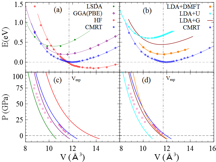
Figure 1: Energy versus Volume (E-V) and Pressure versus Volume (P-V) curves for ferromagnetic bcc iron calculated with different ab initio methods. Plot (a) compares CMRT against weakly interacting methods including LSDA, GGA(PBE) and HF while plot (b) compiles strongly correlated methods, including LDA+DMFT ($U$=4.3eV, $J$=1.0eV)[25], LDA+U ($U$=2.2eV, $J$=1.0eV), LDA+G ($U$=2.2eV, $J$=1.0eV)[29] and CMRT. The corresponding P-V curves are depicted in solid lines in plots (c) and (d). LSDA, PBE, and LDA+U are evaluated with VASP at an automatic K grid of $R_{k}$=40. HF used the identical QUAMBO basis set and K-grid as CMRT. Experimental measurements are symbolized as follows, : solid squares for bcc $\alpha$-Fe phase and empty squares for hcp $\varepsilon$-Fe phase[14, 42]. Vertical adjustments have been made for all the energy curves for a clearer view. Specifically, HF energy is downshifted an extra 5.5eV with respect to CMRT energy in the figure. Vertical dash dotted lines mark the experimental equilibrium volume of the ferromagnetic BCC Fe lattice.

III Results

III.1 Total energy and its related physical quantities

Table 1: BM-EOS fitted equilibrium lattice constant $a_{0}$, bulk modulus $B_{0}$ and the calculated spin magnetic moment $M$ of ferromagnetic BCC Fe obtained by various calculation methods are in comparison with experimental measurements. HF, LDA+U, and CMRT data were calculated in this work, while other data are sourced or adapted from relevant literature: Exp[25], LSDA and GGA(PBE) [15], LDA+DMFT[25], LDA+G[29]. Note that LDA+DMFT utilized $U$=4.3eV and $J$=1.0eV to match the experimental spin magnetic moment value of 2.2$\mu_{B}$ at T=290K. Meanwhile, while there are varied parameter choices for LDA+G in the literature, here it uses $U$=7eV and $J$=1.0eV. Also, note the spin magnetic moment tabulated here is linked to the equilibrium lattice constant specific to each method, and not pegged to the experimental lattice constant.

	Exp	HF	LSDA	PBE	LDA+U	LDA+G	LDA+DMFT	CMRT
$a_{0}$ (Å)	2.867	3.0	2.746	2.833	2.76	2.85	2.853	2.887
$B_{0}$ (GPa)	172	115	245	169	207	160	168	165
$M$ ($\mu_{B}$)	2.2	2.92	2.00	2.2	2.13	2.30	2.2	2.6

In the study of the ferromagnetic ground state of the bulk bcc Fe lattice, energy versus volume (E-V) curves are collected and compared in panel (a) and (b) of Fig 1. These curves contain results from several calculation methods, including HF, LSDA, GGA(PBE), LDA+U, LDA+G, LDA+DMFT and CMRT. Both HF and CMRT calculations share the same QUAMBO basis set, while LSDA, GGA(PBE) and LDA+U are evaluated with plane-wave basis set in this work. GGA data are cross-checked against the published results in Ref. [14]. To complement the E-V curves, the pressure versus volume (P-V) curves extracted from their Birch-Murnaghan Equation of State (BM-EOS) [43] fits are also showcased in panel (c) and (d) of Fig 1, side by side with the experimental measurements, while the accompanying fitted equilibrium volumes and bulk moduli as well as the calculated magnetic moments are collected in Table 1. By examining the intersection points of these curves with the volume axis, we can discern the distribution of equilibrium volumes for each method in relation to the experimental volume. This provides a clear illustration of the exemplary performance of both the GGA and CMRT methods, which operate without the need for adjustable energy parameters, and commendable outcomes of LDA+G and LDA+DMFT with appropriate $U$, $J$ energy parameters adapted. The alignment between the CMRT-generated data and experimental pressure-volume measurements stands out. Specifically, CMRT demonstrates a closer resemblance to experimental outcomes for the bcc iron phase when compared to GGA.

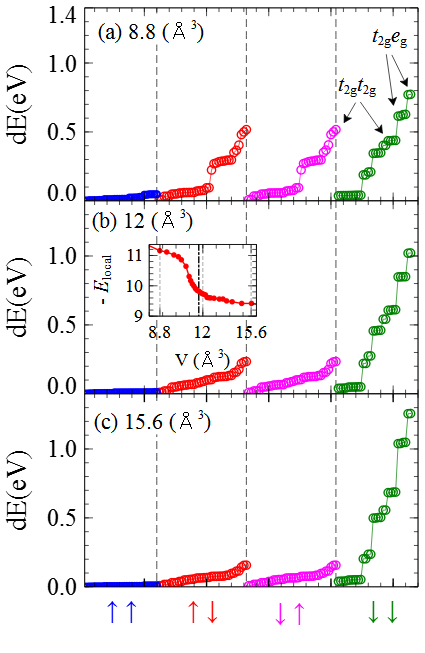
Figure 2: Displayed are the two-body energy components contributing to local energy correction as defined in Eq. 2 at three typical volumes of the BCC iron lattice. Empty circles represent each two-body energy component given by $dE=U_{iiii}^{\alpha\alpha\beta\beta}\left(\bar{n}_{i\alpha\sigma}\bar{n}_{i\beta\sigma^{\prime}}-\left\langle\hat{n}_{i\alpha\sigma}\hat{n}_{i\beta\sigma^{\prime}}\right\rangle\right)$ with $U_{iiii}^{\alpha\alpha\beta\beta}$ local bare Coulomb integral matching $\hat{n}_{i\alpha\sigma}\hat{n}_{i\beta\sigma^{\prime}}$ operator, and are sorted in ascending order on the x-axis for each spin-spin channel at a designated volume. Consequently, symbols located at the same x-coordinate in different volumes may not represent the same operator unless explicitly indicated. Vertical dashed lines distinguish these channels with corresponding consistently colored circles. The up arrow signifies majority spin, while the down arrow indicates minority spin. Prominent local energy correction components pointed with arrows are tagged as $t_{2g}e_{g}$ and $t_{2g}t_{2g},$ representing local two-body operators of $\hat{n}_{t_{2g},\sigma}\hat{n}_{e_{g},\sigma}$ and $\hat{n}_{t_{2g},\sigma}\hat{n}_{t_{2g}^{\prime},\sigma^{\prime}}$ respectively. The inset illustrates the volume dependence of local energy correction induced by electronic correlation and expressed as $-E_{local}$ in the CMRT energy expression of Eq. 1. The thick dashed vertical line there marks the experimental equilibrium volume, while the trio of dashed grid lines point out where energy components were sampled.

One might wonder how local energy corrections resulting from electronic correlations might influence the total energy in CMRT calculations. This particular contribution is encapsulated in $E_{local}$ as seen in Eq. 1. As described by Eq. 2, $E_{local}$ encompasses predominant energy terms arising from $\hat{n}_{i\alpha,\sigma}\hat{n}_{i\beta,\sigma^{\prime}}$ type of two-body operators, where $\alpha$ and $\beta$ represent the set of local correlated orbits. This term delineates the discrepancy between the strict expectation values and their corresponding mean field values. Typically, each term in $E_{local}$ is negative, reflecting diminished Coulomb interaction stemming from the presence of local electronic repulsion. We’ve assigned an additional negative sign to these terms for a clearer visualization in Fig. 2. General understanding might suggest that local correlation energy gain amplifies with increasing volume expansion. Yet, contrary to this notion, the inset of the figure displays a different trend. The root of this behavior can be traced back to the terms that most significantly influence $E_{local},$ as exemplified at three distinct volumes across the experimental equilibrium volume. These individual energy terms are segregated into separate spin-spin channels on the x-axis of Fig. 2: $\uparrow\uparrow$ for majority-majority spin, $\uparrow\downarrow$ for majority-minority spin, and so forth. A closer look reveals that energy corrections from the majority-majority spin channel remain minuscule across the considered terms following the x- axis. The majority-minority spin channel flourishes while it contributes to $E_{local}$ at a reduced volume but diminishes rapidly beyond the experimental volume. Conversely, the minority-minority spin channel possesses a handful of two-body operators that notably amplify their contributions to $E_{local},$ indicating a swift rise in electronic repulsion between specific states. The composite energy correction trajectory, presented in the inset, unveils that the gains from enhanced terms in the minority-minority spin channel fail to offset the dwindling contributions from the majority-minority two-body terms.

III.2 Local Orbital Occupations and Their Fluctuations

A comprehensive examination of the local physics is presented in the ferromagnetic bcc iron lattice using the CMRT method. Fig 3 gives local orbital occupancies on the $t_{2g}$ and $e_{g}$ states of the 3d orbit at a lattice volume of $11.94$ų (or $a=2.88$Å) across various ab initio methods. The orbital occupancies of CMRT align closely with most methods except for HF. For example, using the same QUAMBO local orbit basis set, both LDA and CMRT yield roughly 1.3 electrons in each of the $t_{2g}$ and $e_{g}$ states though CMRT exhibits a slightly greater ordered spin magnetic moment. On the other hand, a discrepancy in the HF orbital occupancy is evident in the minority spin channel, where the $t_{2g}$ state occupation significantly surpasses that of the $e_{g}$ state. This disparity may indicate that the local 3d energy components dominate the HF total energy. More details are provided in the discussion. The CMRT formalism, built upon the HF method, incorporates electronic correlation effects through both renormalizing effective single particle hoppings and rigorously treating local two-body interactions. Such a procedure successfully reduces electron occupancy in the majority spin channel and markedly redistributes electrons between the $t_{2g}$ and $e_{g}$ states in the minority spin channel, yielding more balanced orbital occupancies and tempering the pronouncedly high local spin moment returned by HF.

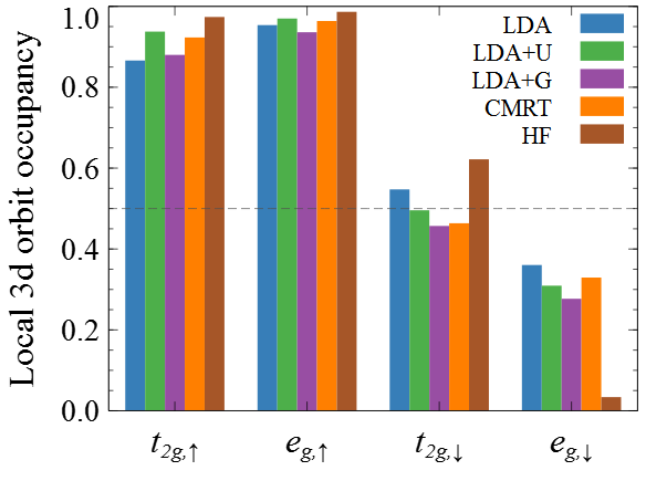
Figure 3: Local charge occupation of th $t_{2g}$ and $e_{g}$ states within the 3d orbit collected from HF, CMRT, LDA+U ($U$=2.3eV, $J$=0.9eV) and LDA+G ($U$=2.5eV, $J$=1.2eV) [30].

To delve deeper into fluctuations, we introduce a local pseudo-charge correlator as

$$\chi_{i\alpha\sigma,i\beta\sigma^{\prime}}=\left\langle\hat{n}_{i\alpha\sigma}\hat{n}_{i\beta\sigma^{\prime}}\right\rangle-\bar{n}_{i\alpha\sigma}\bar{n}_{i\beta\sigma^{\prime}}\text{ for }\left(\alpha\sigma\right)\neq\left(\beta\sigma^{\prime}\right)$$ (8)

This correlator serves as an insightful metric to gauge the electronic correlation between two electronic states effectively capturing how one electron’s presence might influence another’s motion. In essence, this correlator quantifies the deviation in the likelihood of observing a specific electron pair, $\left\langle\hat{n}_{i\alpha\sigma}\hat{n}_{i\beta\sigma^{\prime}}\right\rangle$, which can be thoroughly evaluated within CMRT, from a baseline uncorrelated value, $\bar{n}_{i\alpha\sigma}\bar{n}_{i\beta\sigma^{\prime}}$. When the expectation value is evaluated with a single Slater determinant ground state wavefunction, the result would yield the Hartree term as the baseline value, and a much smaller Fock term if the working basis set possesses the correct lattice and orbital symmetry. Thus, this correlator would nearly vanish in a non-interacting system, as expected for two electrons being uncorrelated.

Introduce local charge and spin (z component only) operators as $\hat{n}$ and $\hat{S}_{z}$ and we can write down the local static charge and spin (z component only) fluctuations, $\chi_{\hat{n}}$ and $\chi_{\hat{S}_{z}},$ as

$$\hat{n}=\sum_{\alpha,\sigma}\hat{n}_{\alpha,\sigma}\Rightarrow\chi_{\hat{n}}=\left\langle\left(\hat{n}-\bar{n}\right)^{2}\right\rangle$$ (9)

$$\hat{S}_{z}=\dfrac{1}{2}\sum_{\alpha,\sigma}\sigma\hat{n}_{\alpha,\sigma}\Rightarrow\chi_{\hat{S}_{z}}=\left\langle\left(\hat{S}_{z}-\bar{S}_{z}\right)^{2}\right\rangle$$ (10)

with $\alpha$ indexing a set of local orbits and $\sigma=\pm 1$ denoting majority and minority spins, respectively. A simple algebra establishes the following relationship between fluctuations and pseudo-charge correlator

$$4\chi_{\hat{S}_{z}}-\chi_{\hat{n}}=4\sum_{\alpha\beta}\left(-\chi_{\alpha\uparrow,\beta\downarrow}\right)$$ (11)

Given a single orbit, the above equation provides a way to gain insights into local double occupancy by taking the difference between the two fluctuations.

Fig. 4 compiles the spin and charge fluctuations from various sets of local orbits and highlights the dominant pseudo-charge correlators. Panels (a) and (b) dissect the fluctuations within all 3d orbits, and within $t_{2g}$ and $e_{g}$ states respectively. The principal variability in spin fluctuation predominantly concerns the $t_{2g}$ states, especially at smaller lattice volumes. Panel (c) provides a clearer perspective on the observation by representing fluctuations for individual states. By noting that local fluctuations of 4S state are not suppressible with increasing electronic correlation, we might reliably classify 4S state to be weakly correlated. Meanwhile, as volume increases, Panel (c) suggests that the $t_{2g}$ and $e_{g}$ states exhibit weak correlation, as indicated by $\left\langle\hat{n}_{i\alpha\uparrow}\hat{n}_{i\alpha\downarrow}\right\rangle\simeq\bar{n}_{i\alpha\uparrow}\bar{n}_{i\alpha\downarrow}$ readily read out from the diminishing difference between the spin and charge fluctuations and with help of Eq. 11. This weak correlation arises from the nearly filled 3d orbits in the majority spin channel. The minority spin channel in the 3d orbits, however, pose to be the chief contributor to local electronic correlations. This observation stems from Fig. 2 and is corroborated by Panel (d) in Fig. 4. This panel showcases $\chi_{i\alpha\sigma,i\beta\sigma^{\prime}}$ adjusted by $\bar{n}_{i\alpha\sigma}\bar{n}_{i\beta\sigma^{\prime}}$ to account for variations in orbital occupation. Such an approach can compare electronic correlations across different state pairs, as is supported by two notable advantages. First, all state pairs maintain their numerical alignment at one with the non-interacting limit. Second, the visualization aptly highlights the few most significant electronic correlations and pinpoints the state pairs that generate them. These predominant correlations between $t_{2g}$ and $e_{g}$ could be the reason for their rebalanced occupations in CMRT which are otherwise significantly skewed in the HF calculation shown in Fig. 3.

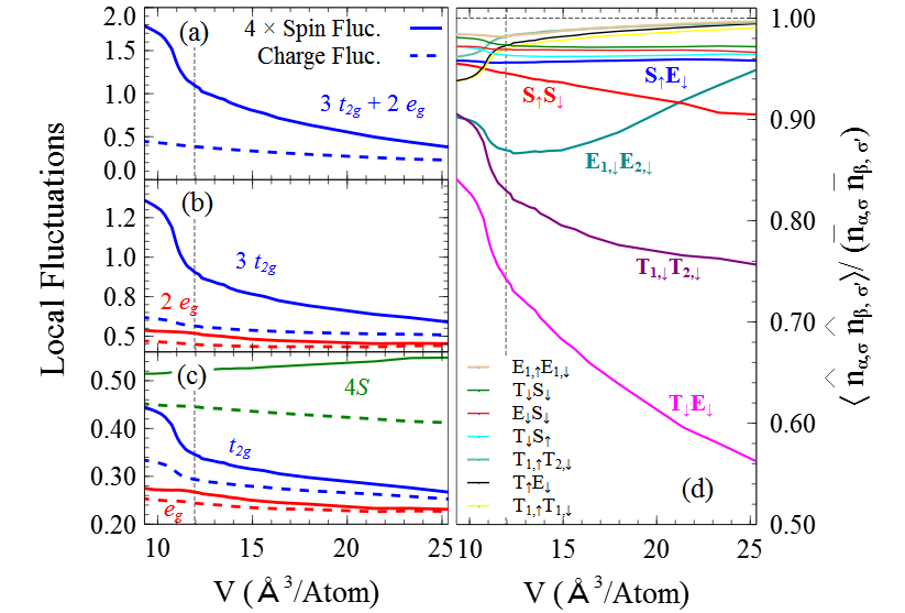
Figure 4: Left panels show local spin and charge fluctuations with different sets of local states. Solid lines show four times spin fluctuation and dashed lines charge fluctuation. Panel (a) selects all $t_{2g}$ and $e_{g}$ states to define the spin and charge operators; panel (b) selects all $t_{2g}$ states as well as all $e_{g}$ states while panel (c) picks up individual $4S,$ $t_{2g}$ and $e_{g}$ states to evaluate their spin and charge fluctuations. The right panel (d) gives comparisons of $\left\langle\hat{n}_{\alpha\sigma}\hat{n}_{\beta\sigma^{\prime}}\right\rangle$ normalized by $\bar{n}_{\alpha\sigma}\bar{n}_{\beta\sigma^{\prime}}$ with $\bar{n}_{\alpha\sigma}=$ $\left\langle\hat{n}_{\alpha\sigma}\right\rangle$. The first five biggest terms have their labels put nearby the curves with matching colors. In contrast, the rest of the terms have their labels collected at the left-bottom corner following roughly the magnitude ordering at a small lattice volume. The curves are consistently labeled with two capital letters denoting a pair of local orbits involved. Specifically, $T,E,S$ denote $t_{2g},$ $e_{g}$ and $4S$ states averaged over their degenerate states, respectively. If the same state is involved in both local orbits, then each letter carries a number to distinguish whether they are the same state. For instance, T_1,↑T_2,↓ denotes $\hat{n}_{\alpha\uparrow}\hat{n}_{\beta\downarrow}$ with $\alpha,\beta\in\left\{t_{2g}\right\}$ but $\alpha\neq\beta,$ while T_1,↑T_1,↓ denotes $\hat{n}_{\alpha\uparrow}\hat{n}_{\alpha\downarrow}$ for $\alpha\in\left\{t_{2g}\right\}$, which is basically the averaged double occupancy of an individual $t_{2g}$ state. The spin index, $\sigma\in\left\{\uparrow,\downarrow\right\},$ denotes majority or minority spins respectively. In both panels, the vertical dotted lines show the CMRT equilibrium volume.

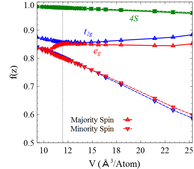
Figure 5: Volume dependence of Gutzwiller renormalization factor, $f\left(z_{\alpha\sigma}\right),$ for both spin channels for selected local states. Blue curves are for $t_{2g},$ red for $e_{g}$ and green for $4S$ states. Solid lines with an upward triangle represent the majority spin, while dashed lines with a downward triangle represent the minority spin. The dashed vertical line indicates the CMRT equilibrium volume with the ferromagnetic bcc iron lattice.

III.3 Normalized Local Charge Fluctuation analysis

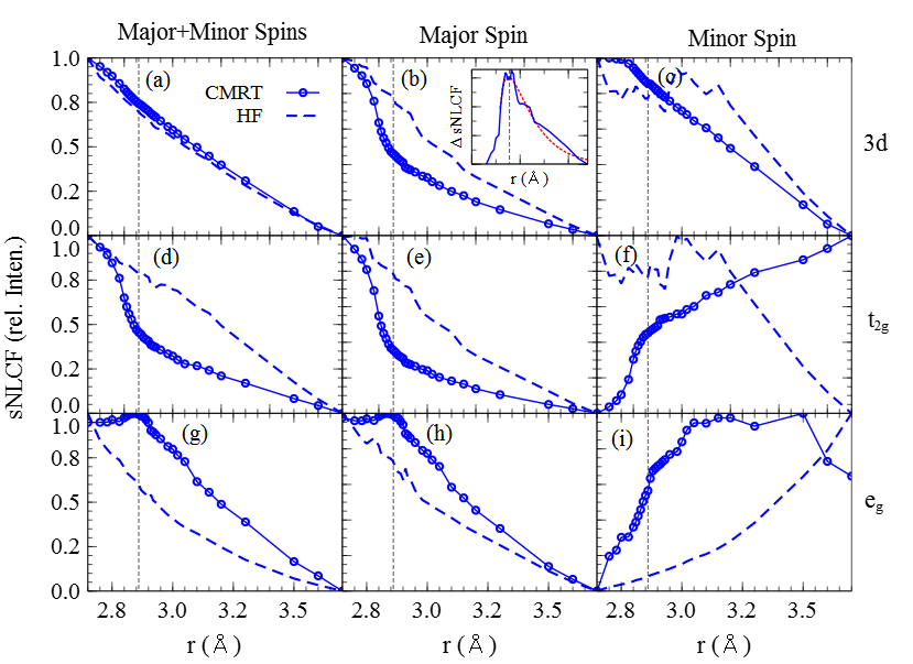
Figure 6: sNLCF results from both HF and CMRT methods are brought side by side in the plots. Labels on the top of the figure show different spin channels of sNLCF in the columns while labels to the right of the figure show the chosen local orbits for sNLCF calculation in each row. Specifically, $3d$ means that all 3d local orbitals of the prechosen spins are selected to define NLCF, $t_{2g}$ and $e_{g}$ denote that a single specific state is chosen for sNLCF calculation. The inset in plot (b) shows lattice constant dependence of difference in sNLCF between HF and CMRT data with the dashed red a smooth fit of the difference to indicate the maximum. The dashed vertical line denotes the equilibrium lattice constant determined from CMRT.

While the Gutzwiller renormalization prefactors for the correlated orbits shown in Fig. 5 reveal some similarity between $t_{2g}$ and $e_{g}$ states in both spin channels, the difference might be explored through the Normalized Local Charge Fluctuation (NLCF), defined as $\chi_{\hat{n}}/\bar{n}^{2}$[39]. We evaluate this metric using CMRT and HF calculations, with HF serving as the reference for electronic correlation. Notable deviations between CMRT and HF indicate additional correlations captured by CMRT. For a balanced comparison, we introduce a standardized NLCF (sNLCF). Given the non-comparability of expectation values in the NLCF definition across methods, we adjusted their range to fall between 0 and 1, considering unique constant shifts.

Fig 6 contrasts sNLCF values from CMRT and HF across subsets of local correlated orbits in a ferromagnetic bcc iron system. This figure presents relative charge fluctuations across different choices of orbits (rows) and spin channels (columns). The top row illustrates CMRT vs. HF for all five 3d orbits, and the middle and bottom rows focus on comparisons for individual $t_{2g}$ and $e_{g}$ states respectively. In interpreting Fig 6, it’s evident that different treatments in electronic correlation between methods yield different sNLCF behaviors. Specifically, the majority spin channel in the second column reveals HF’s near-linear descent as contrasted with CMRT’s well-established curvatures. CMRT either further suppresses or enhances charge fluctuations on top of HF in the $t_{2g}$ or $e_{g}$ states for a better treatment of their electronic correlations. This qualitative difference in $t_{2g}$ and $e_{g}$ treatment supports the distinct correlation nature of both 3d states made in existing literature. The curve in the inset of plot (b), resulting from the difference between HF and CMRT there, peaks near the CMRT equilibrium volume. This might suggest a predominant role of majority spin electrons in shaping the interatomic bonds and the bulk bcc lattice structure.

IV Discussion

We demonstrated that CMRT can correctly predict both the energy versus volume (E-V) and pressure versus volume (P-V) curves for the bulk BCC iron ferromagnetic phase. Furthermore, it yields an equilibrium volume and bulk modulus consistent with experimental findings, as illustrated in Fig. 1. CMRT also produced other credible physical quantities like local orbital renormalization prefactors and orbital occupations. All these suggest that CMRT can capture the essential correlation physics inherent in the 3d orbits of this system. These extra correlations built into CMRT aid in redistributing the system’s kinetic and potential energies, and orbital fillings. While there was analysis indicating that changes in these energy components correlate with the formation of ordered moments[30], we choose not to delve into such intricacies here, given that this information might be method specific. Meanwhile, CMRT predicts a local spin magnetic moment larger than experimental measurements. The local state occupations depicted in Fig 3 reveal that HF-based CMRT still allocates more electrons to the majority spin channel than LSDA/GGA, resulting in an exaggerated local spin magnetic moment. Interestingly, local interaction enhanced LSDA methods, such as DFT+U and DFT+G, display similar local state occupations as CMRT, even though they stem from distinct theoretical backgrounds, namely LSDA and HF.

The local 3d occupation in HF significantly skews towards $t_{2g}$ states in the minority spin channel compared to the other methods, as depicted in Fig. 3. Generally speaking, a preferred occupation on $t_{2g}$ over $e_{g}$ is consistent with the cubic crystal field splitting of 3d orbits[44]. But, this skew in HF calculation seems excessively pronounced. Insight into this phenomenon may be gleaned by examining a simplified model of an isolated atom. This model replicates the local electron filling pattern observed in the ferromagnetic iron state, presupposing nearly fully filled 3d orbits in the majority spin channel and a predetermined number of 3d electrons in the minority spin channel. We closely observe $\hat{n}_{\alpha\sigma}\hat{n}_{\beta\sigma^{\prime}}$ type two-body operators, with $\alpha,\beta\in\left\{t_{2g},e_{g}\right\}$, which are dominant in the energy Hamiltonian and possess very close Coulomb energy coefficients. The classical Coulomb potential energy pertinent to these operators is expressed as follows

$$E_{p}\propto C_{3}^{2}\bar{n}_{t_{2g},\downarrow}\bar{n}_{t_{2g},\downarrow}+6\bar{n}_{t_{2g},\downarrow}\bar{n}_{e_{g},\downarrow}+C_{2}^{2}\bar{n}_{e_{g},\downarrow}\bar{n}_{e_{g},\downarrow}$$ (12)

which might as well be thought of a mean field decomposition on $\hat{n}_{\alpha\sigma}\hat{n}_{\beta\sigma^{\prime}}$ but having the Fock terms dropped as quantum effects. In this equation, $\bar{n}_{t_{2g}\left(e_{g}\right),\downarrow}$ represents local orbital occupation in a $t_{2g}$ or $e_{g}$ state in the minority spin channel, while $C_{n}^{m}$ is the standard binomial coefficient. Simple algebraic manipulation reveals three notable cases[45]. Two extremes, $\left(\bar{n}_{t_{2g},\downarrow},0\right)$ and $\left(0,\bar{n}_{e_{g},\downarrow}\right),$ represent variable-bounded local minima separated by a potential energy maximum, which defines the physically relevant third case holding equal occupation in all 3d orbits for an isolated atom with nearly degenerate orbits. Given this scenario, it is reasonable to hypothesize that the HF solution likely corresponds to one of the two extreme cases in an effort to minimize local potential energy. Confirmation of this hypothesis is obtained by applying HF to the local energy Hamiltonian constructed at a reference site on the BCC iron lattice with a unit cell volume of $25$ų(or $a_{0}=3.7$Å). The HF approach, contingent on specific initial orbital occupations, readily converges to the two extreme cases with vanishing occupation in either type of the 3d states. Comparing these solutions to the actual HF solution for the BCC iron lattice reveals that the extra nonlocal hoppings and interactions left out of the local energy Hamiltonian contribute to electron transitions into the empty states. With local correlation effects incorporated in the HF framework to establish CMRT – which effectively reduces local Coulomb interaction as showcased in Fig. 4 – a greater number of electrons continue to transit into the empty 3d states. This results in a more balanced electron occupation among the 3d states, which would otherwise be energetically discouraged by a local energy Hamiltonian as seen through HF.

Based on the classical potential energy depicted in Eq. 12 and the different orbital occupations between HF and CMRT, two key observations are made. Firstly, local correlation is crucial in reestablishing the correct physical picture in the BCC iron lattice with CMRT. While correlation may reduce nonlocal energy components through Gutzwiller renormalization, the overarching effect is an enhanced nonlocal effect, ensuring a steady electron flow into empty 3d states. Secondly, integrating the exchange-correlation functional into DFT markedly enhances its efficacy, as evidenced here by a correct depiction of the BCC iron lattice. Nevertheless, the similarity in electronic behaviors yielded by both the classical Coulomb repulsion and HF positions HF as a benchmark methodology in comparing treatment on electronic correlation effects, which is purely quantum in nature. These insights might be instrumental in resolving an inconsistent statement made in a QSGW calculation[20] stating that local physics is not relevant for describing BCC iron lattice by taking DFT as its reference.

The local correlated energy, $E_{local},$ as defined in Eq. 2 encapsulates the effect of correlation on the electronic Coulomb interaction energy. When this quantity is subtracted from the CMRT total energy, the equilibrium lattice volume shifts to approximately that of the HF equilibrium volume. This alignment might seem coincidental, given that CMRT and HF converge to distinct ground states with varying orbital occupations in the minority spin channel. Nevertheless, this shifting trend underscores the significance of accurately addressing correlation effects for a precise depiction of a physical system. Segmenting $E_{local}$ into two-body energy components reveals a competition of correlation energy across different spin-spin channels, as illustrated in Fig. 2. The dominant roles of the electronic correlation of $t_{2g}$ and $e_{g}$ states in the minority spin channel are further highlighted in Fig. 4. Concurrently, these figures emphasize the weak correlation present within the majority of spin channels of these states—a perspective somewhat at odds with the insights from $f\left(z\right)$ in Fig. 5. One potential explanation is that $\chi_{\alpha\sigma,\beta\sigma^{\prime}}$ provides static correlation data for two electrons in a system’s final state, which emerges after the culmination of all inherent physical screening and damping effects. In contrast, $f\left(z\right)$ may carry dynamical significance for individual orbits, facilitating quasiparticle motion renormalization and giving rise to necessary screening and damping effects. While $\chi_{\alpha\sigma,\beta\sigma^{\prime}}$ could suggest the ease with which two electrons approach each other, it doesn’t necessarily correlate straightforwardly with the single particle-related Gutzwiller renormalization factor $f\left(z\right)$ under a mean field scenario. Such an interpretation might also reconcile a statement made in a DFT+DMFT calculation emphasizing a strong correlation effect in the majority spin channel[32] by noting an intricate connection between self-energy and Gutzwiller renormalization prefactor[34].

Analysis of local fluctuations and pseudo-charge correlators suggested distinct correlation patterns for 3d orbits in the majority and minority spin channels. A closer look at pseudo-charge correlators associated with $t_{2g}$ and $e_{g}$ states indicates that both orbits exhibit significant interactions within and among themselves in the minority spin channel, without major qualitative differences. Hence, the approach of categorizing $t_{2g}$ and $e_{g}$ states as purely itinerant and localized states or attributing them different electronic characteristics[12] isn’t wholly corroborated by our findings. Subsequent analysis exploring local fluctuation was carried out. While NLCF can be insightful for analyzing electronic localization in strongly correlated systems, it didn’t yield any substantial insights for the bulk BCC iron system. This aligns with the notion that localization-delocalization dynamics are not a primary concern here. On the other hand, by accessing the standardized NLCF for 3d orbits and contrasting them with HF computations, it becomes evident that $t_{2g}$ and $e_{g}$ states have distinct behaviors in the majority spin channel. While they almost retain their local orbit occupations, their local charge fluctuations are modulated in opposing directions, optimizing electronic correlation energy for the CMRT ground state. The profound difference in the behaviors of $t_{2g}$ and $e_{g}$ states within the majority spin channel warrants further investigation.

V Summary

In this study, we expanded the capabilities of CMRT, an entirely ab initio approach for correlated electron systems, to accommodate magnetization by facilitating straightforward spin polarization within the system. We put this formalism to the test, benchmarking it against the established ferromagnetic system of bulk bcc Fe. Interestingly, we found that utilizing spin-independent sum rule energy coefficients yielded the most accurate results in the CMRT total energy computations. This finding is in harmony with a raw ab initio Hamiltonian employing spin-independent energy parameters. We charted the E-V curve for this system, deriving equilibrium attributes like volume and bulk modulus. These values align closely with experimental data and compare positively to other ab initio methodologies. Furthermore, our constructed P-V curve not only mirrors experimental results but also demonstrates better concordance than GGA predictions. Diving deeper, we extensively examined local physical metrics, encompassing local orbit occupation, local spin and charge fluctuations, and local correlation effects using new measures introduced in this study. Our findings pinpointed the primary correlation impact to the 3d orbits within the minority spin channel and highlighted subtle distinctions between $t_{2g}$ and $e_{g}$ states. While the majority spin channel exhibits weak correlation, the behaviors of $t_{2g}$ and $e_{g}$ are notably different. This discrepancy might hinge on the method used, and its physical implications remain unclear.

VI Acknowledgement

Acknowledgement We would like to thank F. Zhang and J. H. Zhang for valuable discussions. This work was supported by the U.S. Department of Energy (DOE), Office of Science, Basic Energy Sciences, Materials Science and Engineering Division, including the computer time support from the National Energy Research Scientific Computing Center (NERSC) in Berkeley, CA. The research was performed at Ames Laboratory, which is operated for the U.S. DOE by Iowa State University under Contract No. DEAC02-07CH11358.

References

- Kittel [2004] C. Kittel, Introduction to Solid State Physics, 8th ed. (Wiley, 2004).
- Kanematsu et al. [2017] K. Kanematsu, S. Misawa, M. Shiga, H. Wada, and H. Wijn, Landolt-Bornstein: Numerical data and functional relationships in science and technology, edited by W. Martienssen, New series, Vol. 32 (Springer, 2017) group III: Condensed Matter Volume 32; Magnetic Properties of Metals, Supplement to Volume 19, Subvolume A, 3d, 4d and 5d Elements, Alloys and Compounds.
- Antonides et al. [1977] E. Antonides, E. C. Jose, and G. A. Sewatzky, Physical Review B 15, 1669 (1977).
- Yin et al. [1977] L. I. Yin, T. Tsang, and I. Adler, Phys. Rev. B 15, 2974 (1977).
- Chandesris et al. [1983] D. Chandesris, J. Lecante, and Y. Petroff, Physical Review B 27, 2630 (1983).
- Şaşıoğlu et al. [2011] E. Şaşıoğlu, C. Friedrich, and S. Blügel, Phys. Rev. B 83, 121101 (2011).
- Gutiérrez and López [1997] A. Gutiérrez and M. F. López, Phys. Rev. B 56, 1111 (1997).
- Wohlfarth [1980] E. Wohlfarth, Iron, cobalt and nickel, in Handbook of Magnetic Materials, Vol. 1, edited by E. Wohlfarth (North-Holland Publishing Company, 1980) p. 1.
- Staunton et al. [1984] J. Staunton, B. Györffy, A. Pindor, G. Stocks, and H. Winter, Journal of Magnetism and Magnetic Materials 45, 15 (1984).
- Stearns [1973] M. B. Stearns, Physical Review B 8 (1973).
- Singh et al. [1991] D. J. Singh, W. E. Pickett, and H. Krakauer, Physical Review B 43, 11628 (1991).
- Katanin et al. [2010] A. A. Katanin, A. I. Poteryaev, A. V. Efremov, A. O. Shorikov, S. L. Skornyakov, M. A. Korotin, and V. I. Anisimov, Phys. Rev. B 81, 045117 (2010).
- Wang et al. [1985] C. S. Wang, B. M. Klein, and H. Krakauer, Physical Review Letters 54, 1852 (1985).
- Stixrude et al. [1994] L. Stixrude, R. E. Cohen, and D. J. Singh, Physical Review B 50, 6442 (1994).
- Kresse and Joubert [1999] G. Kresse and D. Joubert, Physical Review B 59 (1999).
- Schafer et al. [2005] J. Schafer, M. Hoinkis, E. Rotenberg, P. Blaha, and R. Claessen, Physical Review B 72 (2005).
- Gunnarsson [1976] O. Gunnarsson, J. Phys. F: Met. Phys. 6, 587 (1976).
- Yamasaki and Fujiwara [2003] A. Yamasaki and T. Fujiwara, J. Phys. Soc. Jpn. 72, 607 (2003).
- Kotani et al. [2007] T. Kotani, M. v. Schilfgaarde, and S. V. Faleev, Physical Review B 76 (2007).
- Sponza et al. [2017] L. Sponza, P. Pisanti, A. Vishina, D. Pashov, C. Weber, M. van Schilfgaarde, S. Acharya, J. Vidal, and G. Kotliar, Phys. Rev. B 95, 041112 (2017).
- Barreteau et al. [2004] C. Barreteau, M.-C. Desjonquères, A. M. Oleś, and D. Spanjaard, Phys. Rev. B 69, 064432 (2004).
- Belozerov and Anisimov [2014a] A. S. Belozerov and V. I. Anisimov, J. Phys.: Condens. Matter 26, 375601 (2014a).
- Sánchez-Barriga et al. [2009] J. Sánchez-Barriga, J. Fink, V. Boni, I. Di Marco, J. Braun, J. Minár, A. Varykhalov, O. Rader, V. Bellini, F. Manghi, H. Ebert, M. I. Katsnelson, A. I. Lichtenstein, O. Eriksson, W. Eberhardt, and H. A. Dürr, Phys. Rev. Lett. 103, 267203 (2009).
- Lichtenstein et al. [2001] A. I. Lichtenstein, M. I. Katsnelson, and G. Kotliar, Physical Review Letters 87, 067205 (2001).
- Pourovskii et al. [2014] L. V. Pourovskii, J. Mravlje, M. Ferrero, O. Parcollet, and I. A. Abrikosov, Phys. Rev. B 90, 155120 (2014).
- Cococcioni and de Gironcoli [2005] M. Cococcioni and S. de Gironcoli, Phys. Rev. B 71, 035105 (2005).
- Katsnelson and Lichtenstein [1999] M. I. Katsnelson and A. I. Lichtenstein, Journal of Physics: Condensed Matter 11, 1037 (1999).
- Anisimov et al. [2012] V. I. Anisimov, A. S. Belozerov, A. I. Poteryaev, and I. Leonov, Phys. Rev. B 86, 035152 (2012).
- Deng et al. [2008] X. Deng, X. Dai, and Z. Fang, EPL (Europhysics Letters) 83, 37008 (2008).
- Borghi et al. [2014] G. Borghi, M. Fabrizio, and E. Tosatti, Physical Review B 90 (2014).
- Schickling et al. [2016] T. Schickling, J. Bünemann, F. Gebhard, and L. Boeri, Physical Review B 93 (2016).
- Grechnev et al. [2007] A. Grechnev, I. Di Marco, M. I. Katsnelson, A. I. Lichtenstein, J. Wills, and O. Eriksson, Phys. Rev. B 76, 035107 (2007).
- Kvashnin et al. [2015] Y. O. Kvashnin, O. Grånäs, I. Di Marco, M. I. Katsnelson, A. I. Lichtenstein, and O. Eriksson, Phys. Rev. B 91, 125133 (2015).
- Lanatà et al. [2015] N. Lanatà, Y. Yao, C.-Z. Wang, K.-M. Ho, and G. Kotliar, Phys. Rev. X 5, 011008 (2015).
- Liu et al. [2016] C. Liu, J. Liu, Y. X. Yao, P. Wu, C. Z. Wang, and K. M. Ho, J. Chem. Theory Comput. 12, 4806 (2016).
- Zhao et al. [2018] X. Zhao, J. Liu, Y.-X. Yao, C.-Z. Wang, and K.-M. Ho, Phys. Rev. B 97, 075142 (2018).
- Liu et al. [2021a] J. Liu, X. Zhao, Y. Yao, C.-Z. Wang, and K.-M. Ho, Journal of Physics: Condensed Matter 33, 095902 (2021a).
- Belozerov and Anisimov [2014b] A. S. Belozerov and V. I. Anisimov, J. Phys. Condens. Matter 26, 375601 (2014b).
- Liu et al. [2021b] J. Liu, Y. Yao, J. Zhang, K.-M. Ho, and C.-Z. Wang, Phys. Rev. B 104, L081113 (2021b).
- Kresse and Furthmüller [1996] G. Kresse and J. Furthmüller, Phys. Rev. B 54, 11169 (1996).
- Qian et al. [2008] X. Qian, J. Li, L. Qi, C.-Z. Wang, T.-L. Chan, Y.-X. Yao, K.-M. Ho, and S. Yip, Phys. Rev. B 78, 245112 (2008).
- Dewaele et al. [2015] A. Dewaele, C. Denoual, S. Anzellini, F. Occelli, M. Mezouar, P. Cordier, S. Merkel, M. Véron, and E. Rausch, Physical Review B 91 (2015).
- Murnaghan [1944] F. D. Murnaghan, Proc. Natl. Acad. Sci. U.S.A. 30, 244 (1944).
- Blundell [2001] S. Blundell, Magnetism in Condensed Matter (Oxford University Press, Oxford, UK, 2001).
- [45] By assuming to be the initial charge in and supposing a subsequent change of to produce charge in the states, Eq. 12 can be expressed in terms of . Setting the derivative of Eq. 12 to zero yields the physically relevant solution, which is, however, an energy maximum. Note also is bounded between and , which correspond to the two extreme cases.