Cosmic-ray energy reconstruction using machine learning techniques

Abstract

HAWC is a ground-based observatory consisting of $300$ water Cherenkov detectors, which observes the extensive air showers induced by cosmic rays from some TeV to a few PeV and, in particular, gamma rays from $300$ GeV to more than $100$ TeV. One of the crucial features required for a detector of extensive air showers is the estimation of the primary energy of the events to study the spectra of cosmic and gamma rays. For HAWC there are currently two gamma-ray energy estimators: one relies on a ground density parameter, while the other utilizes an artificial neural network. For the cosmic ray energy estimation, there is only one estimator based on maximum likelihood procedures and measurements of the lateral charge distribution of the events. It is worthwhile to update the cosmic-ray energy estimator due to recent improvements of the extensive air shower offline-reconstruction techniques in HAWC. Therefore, we implemented an artificial neural network to reconstruct the primary energy of hadronic events trained with several observables that characterize the air showers. We trained several models and evaluated their performance against the existing cosmic ray energy estimator. In this work, we present the features and performance of these models.

1 Introduction

The High-Altitude Water Cherenkov (HAWC) gamma-ray observatory is located at an altitude of $4100$ m above sea level on the Sierra Negra volcano in Puebla, Mexico. HAWC consists of an array of $300$ water Cherenkov detectors, each instrumented with four photomultiplier tubes (PMTs), covering an area of $22000$ m² [1]. HAWC operates nearly daily with a duty cycle exceeding 95%, and it has a detection rate of approximately $25$ kHz. Given that the majority of the detected shower are cosmic ray, HAWC contributes significantly to the field. For instance, it can investigate the light mass group as reported in [2, 3], or the cosmic-ray anisotropy [4]. One crucial factor in conducting such analyses is having an energy estimator for the primary particle. In previous works, it was used an energy estimator based on a maximum likelihood procedure and the measurements of the lateral charge distribution of the PMT with signals during the event (hereafter, we will refer to this estimation procedure as Likelihood) [2]. With recent improvements in the offline analysis of the HAWC software for shower reconstruction, the cosmic-ray energy estimator needs an update. To accomplish this task, in this contribution, we explore machine learning techniques, which will enable us to build a data-driven model. Section 2 provides details of our model and its training, while, in section  3, the performance of the best trained model is presented and its is compared with the results for the likelihood technique. Finally, we summarize the results of this contribution and provide an overview of our future work (in section 4).

2 Trained model sets

For our analysis, we employed Monte Carlo simulation, which were computed using the standard procedure of HAWC. The CORSIKA package [5] (v740) was used to simulate the interaction between a primary particle and the atmosphere, as well as the resulting extensive air shower. FLUKA [6] and QGSJet-II-04 [7] were employed as our low and high-energy hadronic interaction models, respectively. Eight specie were simulated using a power-law energy spectrum, ranging from 5 GeV to 2 PeV, with an spectral index of $-2$. The GEANT4 [8] package was utilized to simulate the interaction between secondary particles and the HAWC detector. Finally, the official HAWC’s software was employed to reconstruct all shower event.

To train the neural networks, we utilized the TMVA package [9] of ROOT [10]. The architecture of the neural network is defined as 14:10:10:1, where each number represents the number of artificial neurons in each layer. The first layer has fourteen neurons, which is the same number of input variables used. These variables contain information such as the lateral distribution charge (footprint) of the shower, its direction, the percentage of PMTs activated, and the distance of the shower core from the HAWC center. The second and third layers are the hidden layers with ten neurons each, and they use a sigmoid activation function. Finally, the last layer consists of one output neuron used to provide the prediction of the primary particle energy in units of $\log_{10}(E/$GeV). Among various model trained with different input variables, the selected fourteen variables yielded the best results. For training, we established 1000 epochs and utilized the Broyden-Fletcher-Goldfarb-Shannon (BFGS) learning model [9]. During the training stage, two-thirds of the total proton events were used, while the remaining one-third of proton events were reserved for testing, approximately 5 millon of proton event were simulated. Protons were chosen for training the model because of their relative abundances in the intensity of cosmic rays, which is approximately 90% of all detected particles [11].

Multiple sets of neural networks were trained, with each network operating on a different binning scheme. The binning scheme involves two parameters: the fractional signal of activated PMTs during the event ($f_{\text{hit}}$) and the position of the shower core relative to HAWC (for events with shower cores inside HAWC, we use the label in-HAWC, and for events at the border or outside HAWC, the label off-HAWC). Below is a description of three neural network sets used in this work:

• 1st set: A single trained network that predicts the energy for events, with shower core inside and outside of HAWC.

• 2nd set: Two trained networks are utilized. One network predicts the energy for in-HAWC events, while the other network estimates the energy for off-HAWC events.

• 3rd set: Three trained networks are employed for different $f_{\text{hit}}$ bins. The first network is designed for the low $f_{\text{hit}}$ bin range ($2.7\%$ - $22\%$), the second network for the medium $f_{\text{hit}}$ bin range ($22\%$ - $47\%$), and the third network for the high $f_{\text{hit}}$ bin range ($>47\%$).

The optimal model is saved in a file with XML format after the training stage is completed. With this file, we can predict the energy for any event. To evaluate the model’s performance, we use one-third of the total proton events as a test data set and compare the predictions. Figure 1 illustrates the distribution of reconstructed energy versus true energy for the vertical events (zenith angle $<17^{\circ}$) of the three model sets and the Likelihood. The best model is characterized by most events being closer to the identity line (solid dark line), indicating a more accurate prediction. From this results, we found that the third neural network set has the best performance (Figure 1(d)). The Likelihood exhibits two undesired behaviors, both at high energies ($>100$ TeV). The first one is an underestimation of high-energy events, while in the second one is a loss of sensitivity at energies close to 1 PeV and above (resulting in a flat region in the top of Figure 1(a)).

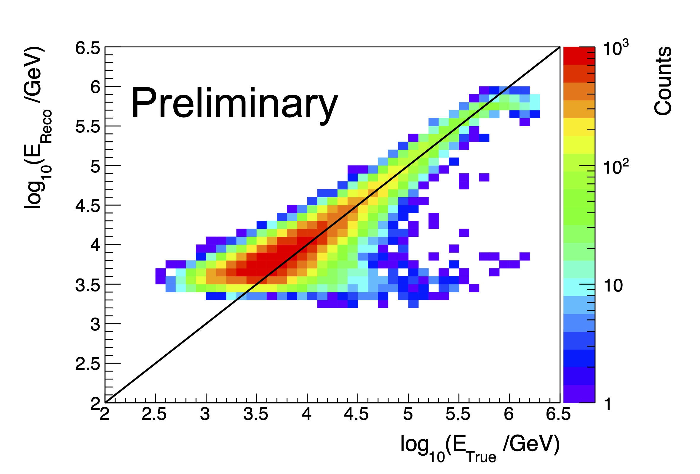
(a) Likelihood

(b) 1st Neural Network set

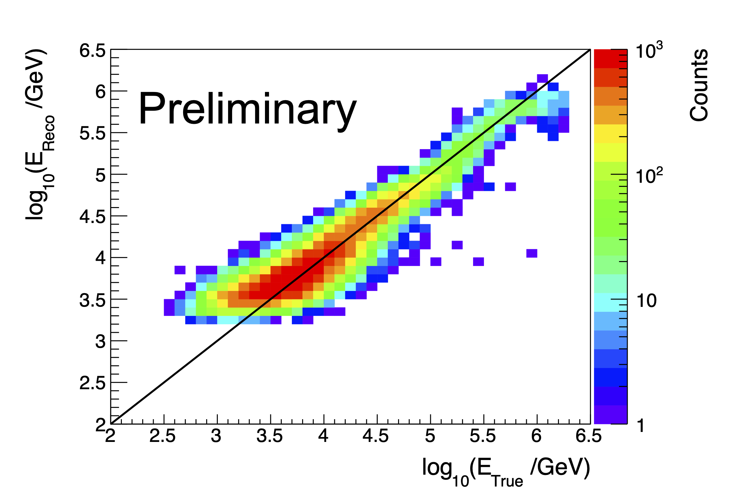
(c) 2nd Neural Network set

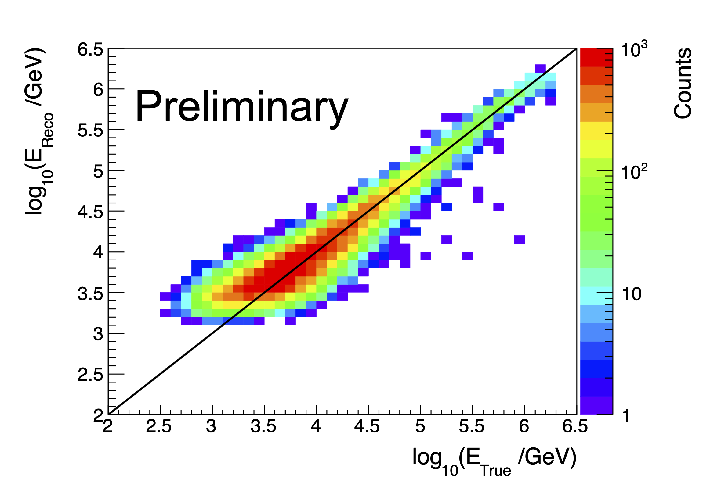
(d) 3rd Neural Network set

Figure 1: A density heatmap is shown, illustrating the true energy versus the reconstructed energy using the Likelihood method (a), and the 1st, 2nd, and 3rd Neural Network sets (b, c, and d respectively) for testing proton-induced showers. The identity line is depicted by the black line.

3 Testing stage

To assess the robustness of our neural network models for other cosmic ray nuclei in the detector, we conducted a test using the iron-induced shower (a heavier component). In figure 2, we compare the resulting performances for the Likelihood and the third neural network set. We observe that, in the case of iron nuclei, the Likelihood exhibits the same behavior as for the case of proton specie. However, the neural network set does not exhibit this behavior at high energies.

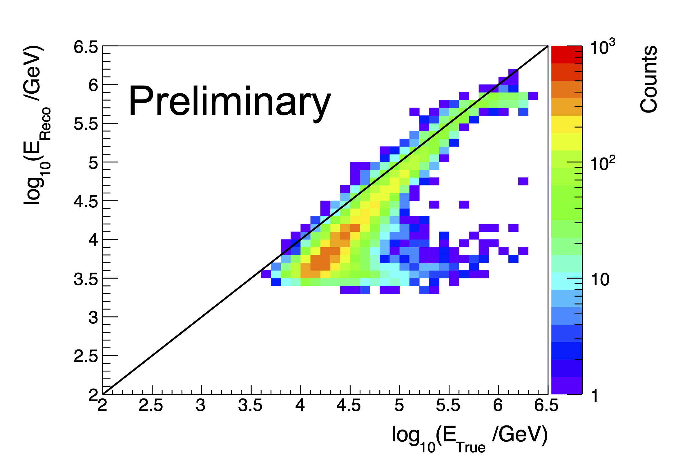
(a) likelihood

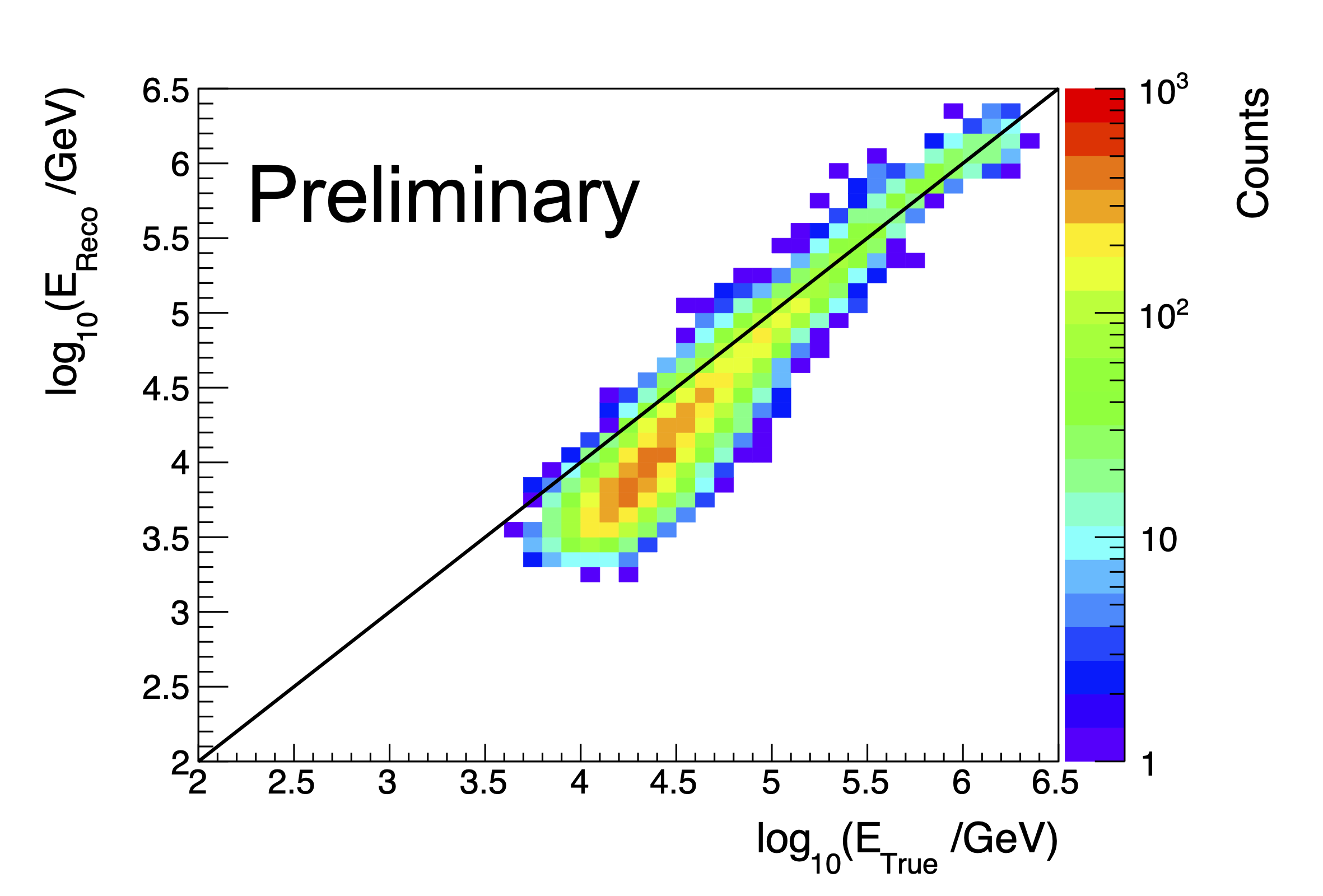
(b) 3rd Neural Network set

Figure 2: A density heatmap is shown, illustrating the true energy versus the reconstructed energy using the Likelihood method (a) and the 3rd Neural Network set (b) for iron-induced showers. The identity line is depicted by the black line.

In order to quantify and evaluate the performance of the models, we calculate the bias, which is defined as the difference between the reconstructed and true energy values, both in logarithmic scale.

$$\text{bias}=\Delta\log_{10}(\text{E})=\log_{10}\left(\text{E}_{\text{Reco}}/\text{GeV}\right)-~{}\log_{10}\left(\text{E}_{\text{True}}/\text{GeV}\right)$$ (1)

We report the mean of the bias distribution for each quarter of a decade stating from $2.0$ ($100$ GeV). These results are presented in Figure 3, considering the proton and iron-induced showers. The bias indicates the proximity of the predictions to the true energy. Between 10 TeV and 100 TeV, most events show a reconstructed energy value lower than the true one for both methods. Between 100 TeV and 1 PeV, both estimators demonstrate an excellent reconstruction, which is consistent with Figures 1 and 2, where the majority of events (indicated by the red zone) are close to the identity line. Finally, beyond 1 PeV, the neural network aligns the events with the identity line, as the bias approaches zero instead of having a significant offset, unlike the Likelihood estimator in the flat region.

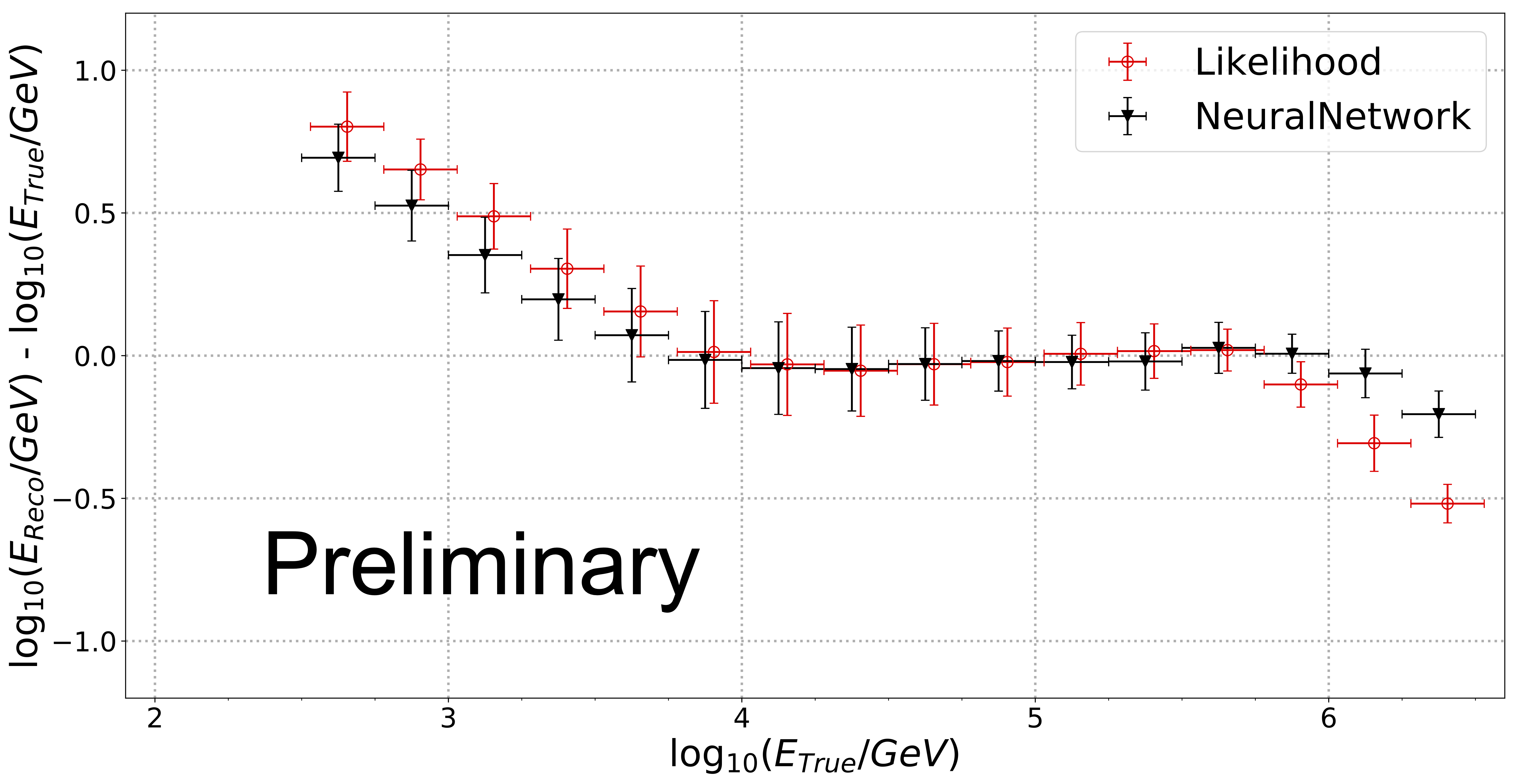
(a) Proton-induced showers

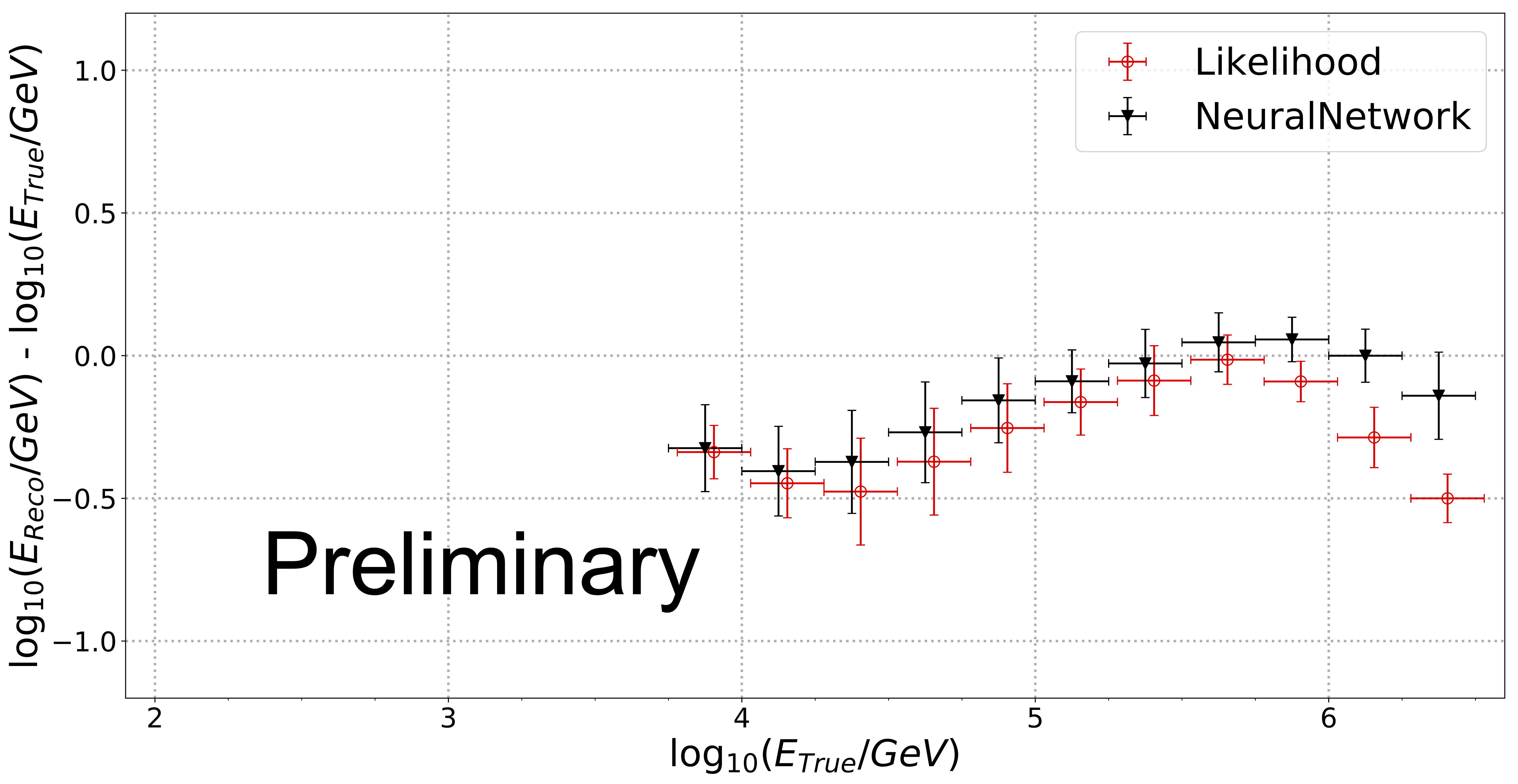
(b) Iron-induced showers

Figure 3: A comparison is made between the bias associated with HAWC’s official energy estimator Likelihood (red) and the 3rd Neural Network set (black) for two specie: (a) proton and (b) iron nuclei.

4 Discussion and Conclusions

In this contribution, we reported the results for the energy estimator of cosmic-ray induced air showers with three neural network sets trained using only proton specie. These sets share the same configuration parameters, such as architecture, number of epochs, and input variables, among characteristics. The difference lies in the number of networks trained within each set. The best model set is achieved when a network is specifically focused on reconstructing events within low, medium, and high fractional hit bins. This set exhibits significant improvements compared to the Likelihood model. In particular, the neural network model reduces the bias at energies close to 1 PeV and also reduce the size of the fluctuation at high energies. We obtain the same behavior when a heavier component, iron nuclei, is used.

Upon exploring the reconstruction of the iron event in the testing stage, it was concluded that it is advisable to train the model with multiple specie instead of just one. This is because there is an offset observed in estimated primary energy with respect to the true value, which is also observed with the Likelihood model. In general, the conclusion of the present study is that the third neural network set proves to be the superior model in comparison with the other ones explored in this work, showing notable improvement, particularly at high energies.

We will explore adding more variables that improve the reconstruction or training the model with a broader range of nuclei instead of relying solely on protons. This approach may help decrease bias in the reconstruction process. Another possibility is to train the models to focus on specific zenith angle bands or explore more sophisticated methods such as deep learning.

Full Authors List: HAWC Collaboration

A. Albert¹, R. Alfaro², C. Alvarez³, A. Andrés⁴, J.C. Arteaga-Velázquez⁵, D. Avila Rojas², H.A. Ayala Solares⁶, R. Babu⁷, E. Belmont-Moreno², K.S. Caballero-Mora³, T. Capistrán⁴, S. Yun-Cárcamo⁸, A. Carramiñana⁹, F. Carreón⁴, U. Cotti⁵, J. Cotzomi²⁶, S. Coutiño de León¹⁰, E. De la Fuente¹¹, D. Depaoli¹², C. de León⁵, R. Diaz Hernandez⁹, J.C. Díaz-Vélez¹¹, B.L. Dingus¹, M. Durocher¹, M.A. DuVernois¹⁰, K. Engel⁸, C. Espinoza², K.L. Fan⁸, K. Fang¹⁰, N.I. Fraija⁴, J.A. García-González¹³, F. Garfias⁴, H. Goksu¹², M.M. González⁴, J.A. Goodman⁸, S. Groetsch⁷, J.P. Harding¹, S. Hernandez², I. Herzog¹⁴, J. Hinton¹², D. Huang⁷, F. Hueyotl-Zahuantitla³, P. Hüntemeyer⁷, A. Iriarte⁴, V. Joshi²⁸, S. Kaufmann¹⁵, D. Kieda¹⁶, A. Lara¹⁷, J. Lee¹⁸, W.H. Lee⁴, H. León Vargas², J. Linnemann¹⁴, A.L. Longinotti⁴, G. Luis-Raya¹⁵, K. Malone¹⁹, J. Martínez-Castro²⁰, J.A.J. Matthews²¹, P. Miranda-Romagnoli²², J. Montes⁴, J.A. Morales-Soto⁵, M. Mostafá⁶, L. Nellen²³, M.U. Nisa¹⁴, R. Noriega-Papaqui²², L. Olivera-Nieto¹², N. Omodei²⁴, Y. Pérez Araujo⁴, E.G. Pérez-Pérez¹⁵, A. Pratts², C.D. Rho²⁵, D. Rosa-Gonzalez⁹, E. Ruiz-Velasco¹², H. Salazar²⁶, D. Salazar-Gallegos¹⁴, A. Sandoval², M. Schneider⁸, G. Schwefer¹², J. Serna-Franco², A.J. Smith⁸, Y. Son¹⁸, R.W. Springer¹⁶, O. Tibolla¹⁵, K. Tollefson¹⁴, I. Torres⁹, R. Torres-Escobedo²⁷, R. Turner⁷, F. Ureña-Mena⁹, E. Varela²⁶, L. Villaseñor²⁶, X. Wang⁷, I.J. Watson¹⁸, F. Werner¹², K. Whitaker⁶, E. Willox⁸, H. Wu¹⁰, H. Zhou²⁷

¹Physics Division, Los Alamos National Laboratory, Los Alamos, NM, USA, ²Instituto de Física, Universidad Nacional Autónoma de México, Ciudad de México, México, ³Universidad Autónoma de Chiapas, Tuxtla Gutiérrez, Chiapas, México, ⁴Instituto de Astronomía, Universidad Nacional Autónoma de México, Ciudad de México, México, ⁵Instituto de Física y Matemáticas, Universidad Michoacana de San Nicolás de Hidalgo, Morelia, Michoacán, México, ⁶Department of Physics, Pennsylvania State University, University Park, PA, USA, ⁷Department of Physics, Michigan Technological University, Houghton, MI, USA, ⁸Department of Physics, University of Maryland, College Park, MD, USA, ⁹Instituto Nacional de Astrofísica, Óptica y Electrónica, Tonantzintla, Puebla, México, ¹⁰Department of Physics, University of Wisconsin-Madison, Madison, WI, USA, ¹¹CUCEI, CUCEA, Universidad de Guadalajara, Guadalajara, Jalisco, México, ¹²Max-Planck Institute for Nuclear Physics, Heidelberg, Germany, ¹³Tecnologico de Monterrey, Escuela de Ingeniería y Ciencias, Ave. Eugenio Garza Sada 2501, Monterrey, N.L., 64849, México, ¹⁴Department of Physics and Astronomy, Michigan State University, East Lansing, MI, USA, ¹⁵Universidad Politécnica de Pachuca, Pachuca, Hgo, México, ¹⁶Department of Physics and Astronomy, University of Utah, Salt Lake City, UT, USA, ¹⁷Instituto de Geofísica, Universidad Nacional Autónoma de México, Ciudad de México, México, ¹⁸University of Seoul, Seoul, Rep. of Korea, ¹⁹Space Science and Applications Group, Los Alamos National Laboratory, Los Alamos, NM USA ²⁰Centro de Investigación en Computación, Instituto Politécnico Nacional, Ciudad de México, México, ²¹Department of Physics and Astronomy, University of New Mexico, Albuquerque, NM, USA, ²²Universidad Autónoma del Estado de Hidalgo, Pachuca, Hgo., México, ²³Instituto de Ciencias Nucleares, Universidad Nacional Autónoma de México, Ciudad de México, México, ²⁴Stanford University, Stanford, CA, USA, ²⁵Department of Physics, Sungkyunkwan University, Suwon, South Korea, ²⁶Facultad de Ciencias Físico Matemáticas, Benemérita Universidad Autónoma de Puebla, Puebla, México, ²⁷Tsung-Dao Lee Institute and School of Physics and Astronomy, Shanghai Jiao Tong University, Shanghai, China, ²⁸Erlangen Centre for Astroparticle Physics, Friedrich Alexander Universität, Erlangen, BY, Germany

References

- [1] A. U. Abeysekara et al. The High-Altitude Water Cherenkov (HAWC) observatory in México: The primary detector. Nuclear Instruments and Methods in Physics Research A, 1052:168253, July 2023.
- [2] R. Alfaro et al. All-particle cosmic ray energy spectrum measured by the HAWC experiment from 10 to 500 TeV. PRD, 96(12):122001, December 2017.
- [3] A. Albert et al. Cosmic ray spectrum of protons plus helium nuclei between 6 and 158 tev from hawc data. Phys. Rev. D, 105:063021, Mar 2022.
- [4] A. U. Abeysekara et al. All-sky Measurement of the Anisotropy of Cosmic Rays at 10 TeV and Mapping of the Local Interstellar Magnetic Field. ApJ, 871(1):96, January 2019.
- [5] D. Heck, , et al. CORSIKA: a Monte Carlo code to simulate extensive air showers. Technical Report Report No. FZKA-6019, 2 1998.
- [6] A Ferrari et al. FLUKA: A multi-particle transport code (program version 2005). Technical Report CERN-2005-010, SLAC-R-773, INFN-TC-05-11, CERN-2005-10, Geneva, 2005.
- [7] S. Ostapchenko. Monte Carlo treatment of hadronic interactions in enhanced Pomeron scheme: QGSJET-II model. PRD, 83(1):014018, January 2011.
- [8] S. Agostinelli et al. GEANT4–a simulation toolkit. Nucl. Instrum. Meth. A, 506:250–303, 2003.
- [9] Andreas Hoecker et al. TMVA: Toolkit for Multivariate Data Analysis. PoS, (ACAT):40, 2007.
- [10] Rene Brun and Fons Rademakers. ROOT — an object oriented data analysis framework. Nuclear Instruments and Methods in Physics Research Section A: Accelerators, Spectrometers, Detectors and Associated Equipment, 389(1):81–86, 1997.
- [11] Thomas K. Gaisser et al. Cosmic Rays and Particle Physics. Cambridge University Press, 1 edition, 1990.