[1]\fnmPanagiotis \surPapastamoulis

[1]\orgdivDepartment of Statistics, \orgnameAthens University of Economics and Business, \orgaddress\street76, Patission str., \cityAthens, \postcode10434, \countryGreece

2]\orgdivDepartment of Sociology, \orgnamePanteion University of Social and Political Sciences, \orgaddress\street136, Syngrou Av., \cityAthens, \postcode17671, \countryGreece

Bayesian inference and cure rate modeling for event history data

papastamoulis@aueb.gr    \fnmFotios S. \surMilienos milienos@panteion.gr * [
Abstract

Estimating model parameters of a general family of cure models is always a challenging task mainly due to flatness and multimodality of the likelihood function. In this work, we propose a fully Bayesian approach in order to overcome these issues. Posterior inference is carried out by constructing a Metropolis-coupled Markov chain Monte Carlo (MCMC) sampler, which combines Gibbs sampling for the latent cure indicators and Metropolis-Hastings steps with Langevin diffusion dynamics for parameter updates. The main MCMC algorithm is embedded within a parallel tempering scheme by considering heated versions of the target posterior distribution. It is demonstrated via simulations that the proposed algorithm freely explores the multimodal posterior distribution and produces robust point estimates, while it outperforms maximum likelihood estimation via the Expectation-Maximization algorithm. A by-product of our Bayesian implementation is to control the False Discovery Rate when classifying items as cured or not. Finally, the proposed method is illustrated in a real dataset which refers to recidivism for offenders released from prison; the event of interest is whether the offender was re-incarcerated after probation or not.

keywords:
MCMC, Bayesian computation, censored data, cured fraction
pacs:
[

MSC Classification]62N02, 62F15, 62N01

1 Introduction

To deal with sources of heterogeneity, a critical issue in modeling time-to-event or event history data, it is not always an easy task; these sources are frequently unobservable (latent) and hence, difficult to manipulate. In this context, researchers typically follow a mixture model approach, especially when the population under study consists of distinct groups, which are considered as the main source of heterogeneity. An emblematic problem of this nature is arising when a group of subjects do not face the event of interest, no matter how long they have been followed up, in contrast to the rest groups of the population; these subjects are mostly called as cured, immune or long-term survivors [1, 2, 3, 4]. It is reasonable to assume the existence of such subjects upon studying, for example, the time-to-divorce (not all couples get divorced; e.g., 5), recidivism (not all offenders commit another crime; e.g., 6, Ch. 5), time-to-default (not all bank customers default; e.g., 7), job mobility (not all employees change their jobs; e.g., 8), the residential mobility (not all people change residence; e.g., 9) or the duration of undergraduate studies (not all students graduate; e.g., 10), among others.

Obviously, the way we split the population into (mutually exclusive and exhaustive) groups, determines the model at hand. For example, if we assume that the population is only composed of two groups, the cured (symb., $I=0$) and susceptibles (symb., $I=1$), then for the population survival function, $S_{P}(t)$, we have

$\displaystyle S_{P}(t)=\pi+(1-\pi)S(t|I=1),$ (1)

where $\pi\in[0,1]$ is the probability of being cured, known as cure rate (incidence), and $S(t|I=1)$ is the survival function of susceptibles (latency); due to the definition of cured subjects, we assume that $S(t|I=0)=1$, for every $t$. In fact, the story of cure modeling started with model (1), the mixture cure model, and the seminal works by Boag [11, 12, 13] which rigorously treated the idea of the existence of cured patients, among those who get a cancer treatment. However, real-life applications make researchers consider different ways of splitting the population into groups, such the one deduced by a competing cause scenario (the roots of this approach can be found in 14, 15, 16, although some earlier works of similar nature could also be met in 17, 18); specifically, suppose that there is a number of competing causes, $M$, with each cause being able (at least, partially) to deliver the event of interest. Then, the population survival function is now given by

$\displaystyle S_{P}(t)=\sum_{m=0}^{L}S_{m}(t)P(M=m)=\pi+\sum_{m=1}^{L}S_{m}(t)P(M=m),$ (2)

where the cure rate is equal to the probability of having zero competing causes (i.e., $\pi=P(M=0)$), while $S_{m}(t)$ is the conditional survival function of subjects with $m$ competing causes (i.e., $S_{m}(t)=P(T>t|M=m)$, with $S_{0}(t)=P(T>t|M=0)=1$, for every $t$) and $L$ is the maximum number of $M$. Hence, under this framework the population is now divided into $L+1$ groups, according to the number of competing causes which could be detected to each subject. Note that the limiting values (as $t\rightarrow\infty$) of the survival functions (1) or (2), are equal to the cure rate, given that $S(t|I=1)$ and $S_{m}(t)$ are proper survival functions (i.e., $\lim_{t\rightarrow\infty}=S(t|I=1)=S_{m}(t)=0$). The mixture model may be seen as a special case of the competing cause cure model (2), by assuming that either the conditional survival function $S_{m}(t)$ is the same for each $m$, i.e., $S_{m}(t)=S(t)$, or $M$ is a Bernoulli random variable, with success probability $1-\pi$.

Although a great part of the literature refers to the study of the mixture cure model, also known as split population model [6, Ch. 5], or limited-failure population model [19, 20], the research interest, at least in the last two decades, is also heavily focused on the competing cause approach and its extensions. Typically, the time needed for the $j$th competing cause to being activated (promotion or progression time) is a random variable, $W_{j}$, and given $M$, $W_{j},j=1,2,\ldots$ are assumed to be independent and identically distributed, and independent of $M$, with a common distribution function $F(t)=1-S(t)$. Then, if the first activation suffices for delivering the event of interest, i.e., $T=\min\{W_{0},\ldots,W_{M}\}$, with $P(W_{0}=\infty)=1$, model (2) becomes

$$S_{p}(t)=\pi+\sum_{m=1}^{L}S(t)^{m}P(M=m)=\varphi(S(t)),$$

where $\varphi(z)$ is the probability generating function of $M$ (e.g., 21). Other approaches generalize the above classical competing cause scenario, by asking, for example, the activation of $r$ out of $M$ causes, for facing the event of interest, with $r\geq 1$ (e.g., 22; some generalizations could also be found in 21, 23, 24, 25). Obviously, the stochastic properties of $M$ play a critical role to the competing cause cure model, and one of the fundamental points for selecting a distribution for $M$ (apart from being non-negative integer-valued random variable, with mass at zero) is whether this distribution is flexible enough, to deal with many different real-life settings. The case where $M$ follows a Poisson distribution, i.e., $S_{p}(t)=\exp\{-\vartheta F(t)\}$, with $\vartheta>0$ being the parameter of the Poisson distribution, known as bounded cumulative hazard or promotion time cure model, is one of the key references in the literature. Having said that, the research interest often focuses on proposing models which contain as special cases the two most studied cure models: the mixture cure model and the promotion time model. This is the case, for example, for the model derived by using the Box-Cox transformation on the population survival function, which is of the form (26)

$\displaystyle S_{P}(t)=\left(1-\gamma\vartheta F(t)\right)^{1/\gamma},\vartheta>0,\gamma\in[0,1],$

with $\vartheta:\rightarrow\delta/(1+\delta\gamma)$, and $\delta>0$ (see also 27, 28, 29, 30, 31, 32). Note that both the promotion time ($\gamma\rightarrow 0$) and mixture cure model ($\gamma=1$) are special cases of this family; $\vartheta$ was given by the above form due to the restriction $\gamma\vartheta\in[0,1]$. To mention that this model was estimated within a Bayesian framework in [26] and posterior inference was performed using Adaptive Rejection Metropolis sampling within the Gibbs sampler [33]. Of similar nature are the models derived by assuming a negative binomial distribution for the number of competing causes (e.g., 34, 35, 36, 37, 38, 39, 40, 41), or a Poisson distribution with random parameter (e.g., 42) or a generalized discrete Linnik distribution (43).

In [44], motivated by the above family of cure models, the next model was introduced

$\displaystyle S_{P}(t)=(1+\gamma c^{\gamma}F(t)^{\lambda})^{-\vartheta/\gamma},\gamma\in\Re,$ (3)

or equivalently

$\displaystyle S_{P}(t)=(1+\gamma\vartheta c^{\gamma\vartheta}F(t)^{\lambda})^{-1/\gamma},\gamma\in\Re,$ (4)

with $\vartheta>0$, $\lambda>0$, and $c=e^{e^{-1}}$. The above model includes among its special cases the promotion time ($\gamma\rightarrow 0$, $\lambda=1$), the negative binomial ($\gamma>0$, $\lambda=1$) and the mixture cure model ($\gamma=-1$, $\lambda=1$; the binomial cure model for $\gamma<0$, $\lambda=1$). Moreover, the case of zero cure rate, i.e., when the population survival function is equal to $1-F(t)$, can also be covered, and it is not found at the boundary of the parameter space, as it is usually happens to other classes of cure models; specifically, this case is described by the scenarios $(\gamma,\lambda,\vartheta)=(-e,1,e)$, under (3), or $(\gamma,\lambda,\vartheta)=(-1,1,e)$, under (4). The parameter estimation was carried out by the Expectation-Maximization (EM) algorithm (under to non-informative random right censoring), wherein the cure indicator among the (right) censored subjects was being treated as the missing information. There are factors, such as, the selection of the initial values of the algorithm (and the corresponding selection for the numerical maximization techniques, involved into the M-step), the flatness and multimodality of the likelihood function (especially, with respect to the parameter $\gamma$), which seem to affect point estimation accuracy; issues seem to exist also with the standard errors, and the coverage probabilities of the confidence intervals, relying on the asymptotic normality of the estimators.

The contribution of this work is to propose a more accurate and robust estimation technique in the class of models introduced by [44], following a fully Bayesian approach. Posterior inference is carried out using Markov chain Monte Carlo (MCMC) sampling. Our MCMC sampler combines standard Metropolis-Hastings moves for single-parameter updates as well as Gibbs sampling [45] for the latent cure indicators. Simultaneous updates of the parameter vector are also implemented using Metropolis-Adjusted Langevin diffusion dynamics [46]. Nevertheless, this scheme will rarely cross low-probability regions; thus, escaping from a minor mode becomes practically unachievable.

We overcome this issue by embedding the main algorithm within a Metropolis-coupled MCMC [47] scheme. Heated versions of the posterior distribution are considered and multiple MCMC chains are ran in parallel. The heated chains boost the tendency of the corresponding MCMC samples to deliberately explore the parameter space due to the fact that their target distribution are flatter compared to the cold chain (target posterior distribution). A Metropolis-Hastings step encourages these parallel chains to exchange states, thus, the cold chain has the potential to switch between modes. An extensive simulation study reveals that the proposed method freely explores the multimodal target posterior distribution and outperforms maximum likelihood estimation via the EM algorithm.

Naturally, classification of subjects as cured or susceptibles is directly available from the MCMC output of the latent status indicators. Furthermore, we are also considering the problem of controlling the False Discovery Rate (FDR) within pre-specified tolerance limits, when the aim of the analysis is to produce a list of “discoveries”, that is, cured individuals. For this purpose we borrow ideas from Bayesian FDR control procedures in statistical bioinformatics [48].

The rest of the paper is organized as follows. Section 2 presents the main ingredients of our Bayesian approach, that is, the complete likelihood after augmenting the model with latent status indicators, as well as the prior assumptions. Section 3 introduces the MCMC sampling schemes for performing posterior inference. Control of the False Discovery Rate is discussed in Section 4. Illustrations of the proposed methodology are given in Section 5 using simulated datasets and comparing against the EM algorithm (Section 5.1); also, a real-life application on recidivism for offenders released from prison (parole/special sentence, work release, or discharge) is presented in Section 5.2. Further details of the implementation and additional results on the simulation study are included in the Appendix.

2 Bayesian model

The estimation of the distribution of susceptibles and the recognition of the cured subjects, are conventionally the most challenging tasks in cure modeling. The study of such populations is commonly characterized by the existence of censored data; this is because the cured subjects do not face the event of interest and therefore, no matter what censoring scheme (research design) has been followed up, their time-to-event are censored and their cure status is unknown (nevertheless, the cure status is being treated as partially known, in some approaches; e.g., 49, 50, 51, 52, 53, 54).

In our approach, we assume that the time-to-event is subject to non-informative random right censoring. Under the classical competing cause scenario and model (4), we further assume that the promotion time $W_{j}$ follows a Weibull distribution; however, as can also be seen by the presentation of our estimation approach, this assumption can effortlessly be relaxed. This is also the case about the role of covariates; although we assume that the set of covariates affects only parameter $\vartheta$, through an exponential link function, the same or another set of covariates (under conditions), could also affect the rest parameters. Furthermore, it is known that there are some identifiability issues with the model under study (see also 44). For example, under (3), we can find two different sets of parameters with exactly the same survival function, given that no covariates have been used in the model; also, when $\gamma=-e$, $\lambda=1$ and the distribution of the promotion time is a Weibull distribution, then a constant cannot be added to the exponential link function of $\vartheta$, in case of using covariates. Here, we use the parametrization (4) and further assuming the existence of a continuous covariate with non-negligible effect on $\vartheta$ through the exponential link function, the identifiability issues are solved.

2.1 Observed likelihood and data augmentation

Denoting by $C_{i}$ and $T_{i}$ the censoring time and time-to-event of the $i$th subject, respectively, our observed data consist of $Y_{i}=\min\{T_{i},C_{i}\}$, along with the censoring indicator $\delta_{i}$, i.e.,

$$\delta_{i}=\begin{cases}1,&\mbox{if }Y_{i}\mbox{ is time-to-event }(T_{i}<C_{i})\\ 0,&\mbox{if }Y_{i}\mbox{ is censoring time }(T_{i}>C_{i})\end{cases},i=1,2,\ldots.$$

The cure indicator,

$$I_{i}=\begin{cases}1,&\mbox{if the $i$th subject is susceptible}\\ 0,&\mbox{if the $i$th subject is cured}\end{cases},i=1,2,\ldots,$$

is therefore a latent variable, among the censored subjects. Thus, although we know that every uncensored subject is susceptible (i.e., $i\in\Delta_{1}\Rightarrow I_{i}=1$, where $\Delta_{1}=\{i:\delta_{i}=1\}$), this is not the case for every censored subject, which may either be cured or not (i.e., $i\in\Delta_{0}\Rightarrow I_{i}=1$ or $I_{i}=0$, where $\Delta_{0}=\{i:\delta_{i}=0\}$).

Hence, from $n$ independent pairs $(\delta_{i},y_{i})$, as well as a set of covariates ${\boldsymbol{x}}=({\boldsymbol{x}}_{1},\ldots,{\boldsymbol{x}}_{n})$, the likelihood function can be written as

$\displaystyle L=L({\boldsymbol{\theta}};{\boldsymbol{y}},{\boldsymbol{x}},{\boldsymbol{\Delta}})=\prod_{i=1}^{n}f_{P}(y_{i};{\boldsymbol{\theta}},{\boldsymbol{x}}_{i})^{\delta_{i}}S_{P}(y_{i};{\boldsymbol{\theta}},{\boldsymbol{x}}_{i})^{1-\delta_{i}},$

where ${\boldsymbol{y}}=(y_{1},\ldots,y_{n})$, ${\boldsymbol{\Delta}}=(\delta_{1},\ldots,\delta_{n})$, and $f_{P}(y_{i};{\boldsymbol{\theta}},{\boldsymbol{x}}_{i})$ denotes the population density function, i.e., $f_{P}(y;{\boldsymbol{\theta}},{\boldsymbol{x}})=-\partial S_{P}(y;{\boldsymbol{\theta}},{\boldsymbol{x}})/\partial y$, with

$$S_{P}(y;{\boldsymbol{\theta}},{\boldsymbol{x}})=(1+\gamma\vartheta({\boldsymbol{x}})c^{\gamma\vartheta({\boldsymbol{x}})}F(y;{\boldsymbol{\theta}})^{\lambda})^{-1/\gamma}$$

while, $\boldsymbol{\theta}$ stands for the vector of model parameters.

The complete likelihood function (assuming that the cure indicator for the censored group is observed) reads

$\displaystyle L_{c}({\boldsymbol{\theta}};{\boldsymbol{y}},{\boldsymbol{x}},{\boldsymbol{\Delta}},{\boldsymbol{I}})=$ $\displaystyle\prod_{i\in\Delta_{1}}(1-p_{0}({\boldsymbol{x}}_{i};{\boldsymbol{\theta}}))\prod_{i\in\Delta_{1}}f_{U}(y_{i};{\boldsymbol{\theta}},{\boldsymbol{x}}_{i})$
$\displaystyle\prod_{i\in\Delta_{0}}p_{0}({\boldsymbol{x}}_{i};{\boldsymbol{\theta}})^{1-I_{i}}\prod_{i\in\Delta_{0}}\left\{(1-p_{0}({\boldsymbol{x}}_{i};{\boldsymbol{\theta}}))S_{U}(y_{i};{\boldsymbol{\theta}},{\boldsymbol{x}}_{i})\right\}^{I_{i}},$

with ${\boldsymbol{I}}=(I_{1},\ldots,I_{n})$, and $p_{0}({\boldsymbol{x}}_{i};{\boldsymbol{\theta}})=(1+\gamma\vartheta({\boldsymbol{x}}_{i})c^{\gamma\vartheta({\boldsymbol{x}}_{i})})^{-1/\gamma}$ being the cure rate, while

$\displaystyle S_{U}(y_{i};{\boldsymbol{\theta}},{\boldsymbol{x}}_{i})=\frac{S_{P}(y_{i};{\boldsymbol{\theta}},{\boldsymbol{x}}_{i})-p_{0}({\boldsymbol{x}}_{i};{\boldsymbol{\theta}})}{1-p_{0}({\boldsymbol{x}}_{i};{\boldsymbol{\theta}})},f_{U}(y_{i};{\boldsymbol{\theta}},{\boldsymbol{x}}_{i})=\frac{f_{P}(y_{i};{\boldsymbol{\theta}},{\boldsymbol{x}}_{i})}{1-p_{0}({\boldsymbol{x}}_{i};{\boldsymbol{\theta}})},$

are the (proper) survival and probability density functions of susceptibles, respectively.

2.2 Prior assumptions

Let us assume that the promotion times are Weibull distributed (as we mentioned, this assumption could effortlessly be relaxed), with cumulative distribution function

$$F(y_{i};\alpha_{1},\alpha_{2})=1-\exp\{-(\alpha_{1}y_{i})^{\alpha_{2}}\},\alpha_{1}>0,\alpha_{2}>0.$$

Furthermore, supposing that a set of $k$ covariates affects the parameter $\vartheta>0$ of model (4), through the exponential function, we have

$$\vartheta=\vartheta({\boldsymbol{x}}_{i})=\exp\{{\boldsymbol{\beta}}{\boldsymbol{x}}_{i}^{\prime}\}=\exp\{\beta_{0}+\beta_{1}x_{1}+\ldots+\beta_{k}x_{k}\},$$

where ${\boldsymbol{\beta}}=(\beta_{0},\beta_{1},\ldots,\beta_{k})$, ${\boldsymbol{x}}_{i}=(1,x_{1i},\ldots,x_{ki})$, and $k\geq 1$. Thus, given the vector of parameters $\boldsymbol{\theta}=(\gamma,\lambda,\alpha_{1},\alpha_{2},{\boldsymbol{\beta}})$ and the (fixed) covariates $\boldsymbol{x}$, the joint density of the complete data $(\boldsymbol{y},\boldsymbol{I})$ is

$\displaystyle f(\boldsymbol{y},\boldsymbol{I}|\boldsymbol{\Delta},\boldsymbol{\theta},\boldsymbol{x})=$ $\displaystyle\prod_{i\in\Delta_{1}}(1-p_{0}(\boldsymbol{x}_{i};\boldsymbol{\theta}))\prod_{i\in\Delta_{1}}f_{U}(y_{i};\boldsymbol{\theta},\boldsymbol{x}_{i})$
$\displaystyle\prod_{i\in\Delta_{0}}p_{0}(\boldsymbol{x}_{i};\boldsymbol{\theta})^{1-I_{i}}\prod_{i\in\Delta_{0}}\left\{(1-p_{0}(\boldsymbol{x}_{i};\boldsymbol{\theta}))S_{U}(y_{i};\boldsymbol{\theta})\right\}^{I_{i}}.$ (5)

All parameters are assumed a-priori independent, thus, the general form of the joint prior distribution factorizes as $\pi(\boldsymbol{\theta})=\pi(\gamma)\pi(\lambda)\pi(\alpha_{1})\pi(\alpha_{2})\pi(\boldsymbol{\beta})$. More specifically, each parameter is a-priori distributed as follows:

$\displaystyle\gamma$ $\displaystyle\sim f_{\gamma}(a_{\gamma},b_{\gamma})$ (6)
$\displaystyle\alpha_{1}$ $\displaystyle\sim\mathcal{IG}(a_{1},b_{1})$
$\displaystyle\alpha_{2}$ $\displaystyle\sim\mathcal{IG}(a_{2},b_{2})$
$\displaystyle\lambda$ $\displaystyle\sim\mathcal{IG}(a_{\lambda},b_{\lambda})$
$\displaystyle\boldsymbol{\beta}=(\beta_{0},\beta_{1},\ldots,\beta_{k})^{\top}$ $\displaystyle\sim\mathcal{N}_{p}(\boldsymbol{\mu},\Sigma),$

where $a_{\gamma}>0$, $b_{\gamma}>0$, $a_{1}>0$, $a_{2}>0$, $b_{1}>0$, $b_{2}>0$, $a_{\lambda}>0$, $b_{\lambda}>0$, $\boldsymbol{\mu}\in\mathbb{R}^{k+1}$, $\Sigma\in\mathcal{M}_{+}$, with $\mathcal{M}_{+}$ denoting the space of $(k+1)\times(k+1)$ symmetric positive definite matrices ($G(\cdot,\cdot),\mathcal{IG}(\cdot,\cdot)$ and $\mathcal{N}_{p}(\cdot,\cdot)$, denote the Gamma (shape, rate), inverse Gamma and $p$th dimensional normal distribution, respectively). The prior distribution $f_{\gamma}(a_{\gamma},b_{\gamma})$ of $\gamma$ denotes an equally weighted mixture of a $\mathcal{G}(a_{\gamma},b_{\gamma})$ distribution and its reflection towards 0, that is,

$\displaystyle\gamma=\begin{cases}\hfill Z,\quad&\mbox{with probability }1/2\\ -Z,\quad&\mbox{with probability }1/2\end{cases}$

where $Z\sim\mathcal{G}(a_{\gamma},b_{\gamma})$.

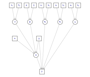
The prior assumptions stated above are based on adopting continuous distributions on the parameter space. Although this seems a reasonable approach, it is not always the case in cure modeling theory; for example, we refer the reader to [26] where a discrete prior distribution was assigned to $\gamma$, under the Box-Cox transformation cure model, in order to avoid numerical problems. The main reason for choosing prior (6) is that it allows greater flexibility compared to a unimodal distribution (e.g. a normal distribution centered at zero). For the remaining parameters, we use absolutely continuous prior distributions on their support, something that can be achieved by inverse Gamma ($\mathcal{IG}$) distributions for the positive parameters and normal distributions for the regression coefficients ($\boldsymbol{\beta}$). In our applications we consider two distinct sets of hyperparameter values, corresponding to “vague” and “regularized” setups. The reader is referred to Appendix A for more details. Figure 1 illustrates the previous hierarchical cure model as a directed acyclic graph, where circles are used to denote unobserved (partially, at least) random variables and squares represent fixed/observed quantities.

Refer to caption
Figure 1: Directed acyclic graph representation of the hierarchical Bayesian cure model.

3 MCMC sampling schemes

The joint posterior distribution of latent indicator variables and model parameters, up to a normalizing constant, is written as

$\displaystyle\pi(\boldsymbol{\theta},\boldsymbol{I}|\boldsymbol{\Delta},\boldsymbol{y},\boldsymbol{x})\propto$ $\displaystyle f(\boldsymbol{y},\boldsymbol{I}|\boldsymbol{\Delta},\boldsymbol{\theta},\boldsymbol{x})\pi(\boldsymbol{\theta})$
$\displaystyle\propto$ $\displaystyle\prod_{i\in\Delta_{1}}(1-p_{0}(\boldsymbol{x}_{i};\boldsymbol{\theta}))\prod_{i\in\Delta_{1}}f_{U}(y_{i},\boldsymbol{x}_{i})\prod_{i\in\Delta_{0}}p_{0}(\boldsymbol{x}_{i};\boldsymbol{\theta})^{1-I_{i}}$
$\displaystyle\prod_{i\in\Delta_{0}}\left\{(1-p_{0}(\boldsymbol{x}_{i};\boldsymbol{\theta}))S_{U}(y_{i},\boldsymbol{x}_{i};\theta)\right\}^{I_{i}}\pi(\boldsymbol{\theta}).$ (7)

In the following sections we will also consider the problem of simulating an MCMC sample which targets a power of the original posterior distribution. For a given constant $0\leqslant h\leqslant 1$, we define the corresponding heated posterior distribution $\pi(\boldsymbol{\theta},\boldsymbol{I}|\boldsymbol{\Delta},\boldsymbol{y},\boldsymbol{x})^{h}$, that is,

$\displaystyle\pi(\boldsymbol{\theta},\boldsymbol{I}|\boldsymbol{\Delta},\boldsymbol{y},\boldsymbol{x})^{h}\propto$ $\displaystyle f(\boldsymbol{y},\boldsymbol{I}|\boldsymbol{\Delta},\boldsymbol{\theta},\boldsymbol{x})^{h}\pi(\boldsymbol{\theta})^{h}$
$\displaystyle\propto$ $\displaystyle\prod_{i\in\Delta_{1}}(1-p_{0}(\boldsymbol{x}_{i};\boldsymbol{\theta}))^{h}\prod_{i\in\Delta_{1}}f_{U}(y_{i},\boldsymbol{x}_{i})^{h}\prod_{i\in\Delta_{0}}p_{0}(\boldsymbol{x}_{i};\boldsymbol{\theta})^{h(1-I_{i})}$
$\displaystyle\prod_{i\in\Delta_{0}}\left\{(1-p_{0}(\boldsymbol{x}_{i};\boldsymbol{\theta}))S_{U}(y_{i},\boldsymbol{x}_{i};\theta)\right\}^{hI_{i}}\pi(\boldsymbol{\theta})^{h}.$ (8)

Note that

$\displaystyle f(\boldsymbol{y},\boldsymbol{I}|\boldsymbol{\Delta},\boldsymbol{\theta},\boldsymbol{x})^{h}\propto\dot{f}_{h}(\boldsymbol{y},\boldsymbol{I}|\boldsymbol{\Delta},\boldsymbol{\theta},\boldsymbol{x}):=$
$\displaystyle\prod_{i\in\Delta_{1}}(1-p_{0}(\boldsymbol{x}_{i};\boldsymbol{\theta}))^{h}\prod_{i\in\Delta_{1}}f_{U}(y_{i},\boldsymbol{x}_{i})^{h}\prod_{i\in\Delta_{0}}p_{0}(\boldsymbol{x}_{i};\boldsymbol{\theta})^{h(1-I_{i})}\prod_{i\in\Delta_{0}}\left\{(1-p_{0}(\boldsymbol{x}_{i};\boldsymbol{\theta}))S_{U}(y_{i},\boldsymbol{x}_{i};\theta)\right\}^{hI_{i}}$ (9)

as well as

$\displaystyle\pi(\boldsymbol{\theta})^{h}\propto\dot{\pi}_{h}(\gamma)\dot{\pi}_{h}(\lambda)\dot{\pi}_{h}(\alpha_{1})\dot{\pi}_{h}(\alpha_{2})\dot{\pi}_{h}(\boldsymbol{\beta})$

where we have also defined

$\displaystyle\dot{\pi}_{h}(\gamma)$ $\displaystyle:=|\gamma|^{\alpha_{\gamma}-1}\exp\{-\beta_{\gamma}|\gamma|\}\mathrm{I}_{\mathbb{R}^{\star}}(\gamma)$
$\displaystyle\dot{\pi}_{h}(\lambda)$ $\displaystyle:=\frac{1}{\lambda^{h(\alpha_{\lambda}+1)}}\exp\left\{-\frac{h\beta_{\lambda}}{\lambda}\right\}\mathrm{I}_{(0,\infty)}(\lambda)$
$\displaystyle\dot{\pi}_{h}(\alpha_{1})$ $\displaystyle:=\frac{1}{\alpha_{1}^{h(a_{1}+1)}}\exp\left\{-\frac{hb_{1}}{\alpha_{1}}\right\}\mathrm{I}_{(0,\infty)}(\alpha_{1})$
$\displaystyle\dot{\pi}_{h}(\alpha_{2})$ $\displaystyle:=\frac{1}{\alpha_{2}^{h(a_{2}+1)}}\exp\left\{-\frac{hb_{2}}{\alpha_{2}}\right\}\mathrm{I}_{(0,\infty)}(\alpha_{2})$
$\displaystyle\dot{\pi}_{h}(\boldsymbol{\beta})$ $\displaystyle:=\exp\left\{-\frac{h}{2}(\boldsymbol{\beta}-\boldsymbol{\mu})^{\top}\Sigma^{-1}(\boldsymbol{\beta}-\boldsymbol{\mu})\right\}\mathrm{I}_{\mathbb{R}^{p}}(\boldsymbol{\beta}),$

with $\mathrm{I}_{A}(\cdot)$ denoting the indicator function of $A$.

3.1 Metropolis-Hastings and MALA updates of parameters

The components of the parameter vector $\boldsymbol{\theta}=(\gamma,\lambda,\alpha_{1},\alpha_{2},\boldsymbol{\beta})$ are updated using two schemes. First, a Metropolis-Hastings kernel updates each component separately. Second, a Metropolis-Adjusted Langevin diffusion updates simultaneously all of them. These moves generate candidate states by suitable proposal distributions, which are then accepted or rejected according to certain acceptance probabilities.

More specifically, the first part of our MCMC sampler consists of standard Metropolis-Hastings updates. In brief, we have used a normal proposal distribution for $\gamma$, log-normal distributions for $\alpha_{1}$, $\alpha_{2}$ and $\lambda$ and a multivariate normal proposal for $\boldsymbol{\beta}$ (see Appendix B.1 for detailed descriptions of these moves).

The previous Metropolis-Hastings steps are based on random walk proposals per parameter and it is well known that may lead to slow-mixing and poor convergence of the MCMC sampler. In order to overcome this issue, we also use a proposal distribution which is based on the gradient information of the (heated) posterior distribution, conditional on the current value of latent status indicators. The Metropolis Adjusted Langevin Algorithm (MALA) [46, 55, 56] is based on the following proposal mechanism

$$\tilde{\boldsymbol{\theta}}=\boldsymbol{\theta}+\tau\nabla\log\pi^{h}(\boldsymbol{\theta}|\boldsymbol{\Delta},\boldsymbol{y},\boldsymbol{x},\boldsymbol{I})+\sqrt{2\tau}\boldsymbol{\varepsilon},$$ (10)

where $\boldsymbol{\varepsilon}\sim\mathcal{N}(\boldsymbol{0},\mathcal{I}_{p+4})$ and $\nabla\log\pi^{h}(\boldsymbol{\theta}|\boldsymbol{\Delta},\boldsymbol{y},\boldsymbol{x},\boldsymbol{I})$ denotes the gradient vector of the logarithm of the full conditional heated posterior distribution of $\boldsymbol{\theta}$ ($\mathcal{I}_{p+4}$ stands for the $(p+4)\times(p+4)$ identity matrix; see Appendices B.2 and C for a detailed description of the implementation).

3.2 Gibbs update for latent cured status indicators

Every recorded time-to-event ($i\in\Delta_{1}$) implies that the corresponding subject is susceptible ($I_{i}=1$), thus, the full conditional distribution in this case is a degenerate distribution at $1$, i.e.,

$\displaystyle\mathrm{P}(I_{i}=1|\delta_{i}=1)=1.$

For the remaining (censored) times, according to Equation (7), we have that

$\displaystyle\mathrm{P}(I_{i}=1|\delta_{i}=0,\boldsymbol{\theta},\boldsymbol{y},\boldsymbol{x})$ $\displaystyle\propto(1-p_{0}(\boldsymbol{x}_{i};\boldsymbol{\theta}))S_{U}(y_{i},\boldsymbol{x}_{i};\theta)=S_{P}(y_{i},x_{i};\boldsymbol{\theta})-p_{0}(x_{i};\boldsymbol{\theta})$
$\displaystyle\mathrm{P}(I_{i}=0|\delta_{i}=0,\boldsymbol{\theta},\boldsymbol{y},\boldsymbol{x})$ $\displaystyle\propto p_{0}(x_{i};\boldsymbol{\theta}).$

In summary, the full conditional distribution of latent status indicators is

$$I_{i}|(\delta_{i},\boldsymbol{\theta},\boldsymbol{y},\boldsymbol{x})\sim\mathcal{B}(1,\rho_{i}),\quad\mbox{independent for }i=1,\ldots,n$$

where

$$\rho_{i}=\begin{cases}1,&\quad\mbox{ if }\delta_{i}=1\\ \dfrac{S_{P}(y_{i},x_{i};\boldsymbol{\theta})-p_{0}(x_{i};\boldsymbol{\theta})}{S_{P}(y_{i},x_{i};\boldsymbol{\theta})},&\quad\mbox{ if }\delta_{i}=0\end{cases}$$

($\mathcal{B}(1,\rho_{i})$ stands for the binomial distribution with parameters, 1 and $\rho_{i}$).

Generalizing this to the case where the target distribution is the heated posterior $\pi(\boldsymbol{\theta},\boldsymbol{I}|\boldsymbol{\Delta},\boldsymbol{y},\boldsymbol{x})^{h}$ in Equation (8) for some $h\in[0,1]$, it readily follows that the relevant full conditional distribution becomes

$$I_{i}|(\delta_{i},\boldsymbol{\theta},\boldsymbol{y},\boldsymbol{x})\sim\mathcal{B}(1,w_{hi}),\quad\mbox{independent for }i=1,\ldots,n$$ (11)

where

$$w_{hi}=\begin{cases}1,&\quad\mbox{ if }\delta_{i}=1\\ \dfrac{\left\{S_{P}(y_{i},x_{i};\boldsymbol{\theta})-p_{0}(x_{i};\boldsymbol{\theta})\right\}^{h}}{\left\{S_{P}(y_{i},x_{i};\boldsymbol{\theta})-p_{0}(x_{i};\boldsymbol{\theta})\right\}^{h}+p_{0}(x_{i};\boldsymbol{\theta})^{h}},&\quad\mbox{ if }\delta_{i}=0\end{cases}.$$

Naturally, when $h=1$ (which corresponds to the original posterior distribution) the expression for $w_{hi}$ collapses to $\rho_{i}$ defined above.

Combining the single site Metropolis-Hastings updates, the MALA proposal and the Gibbs sampling step for the latent status gives rise to the Metropolis-Adjusted Langevin Within Gibbs MCMC sampling scheme summarized in Algorithm 1. Notice that in each iteration, a random selection is made between the simple Metropolis-Hastings move (Step 1) and the MALA proposal (Step 2), with corresponding probabilities equal to $p_{1}$ and $1-p_{1}$, respectively. The value of $p_{1}=0.5$ is chosen as default in our applications.

Input : Data $\boldsymbol{y},\boldsymbol{x},\boldsymbol{\Delta}=(\boldsymbol{\Delta}_{0},\boldsymbol{\Delta}_{1})$
Prior hyper-parameters $\mu_{\gamma},\sigma^{2}_{\gamma},\alpha_{\lambda},\beta_{\lambda},a_{1},b_{1},a_{2},b_{2},\boldsymbol{\mu},\Sigma$
Scale parameters of the proposal distributions η_h := (s^2_g(h), s^2_λ(h),s^2_α_1(h),s^2_α_2(h), s^2_g(h),ν_(h), τ_(h))
(Inverse) temperature of the target distribution $0\leqslant h\leqslant 1$
Number of MCMC iterations $m$
Optional vector of starting values $(\boldsymbol{I}^{(0)},\boldsymbol{\theta}^{(0)})$
Output :  MCMC sample $\{\boldsymbol{\xi}_{h}^{(t)}=(\boldsymbol{I}^{(t)},\boldsymbol{\theta}^{(t)}),t=1,\ldots,m\}$
Step 0: Initialization
       if Starting values not supplied then
             Obtain random starting values $\boldsymbol{\xi}_{h}^{(0)}=(\boldsymbol{\theta}^{(0)},\boldsymbol{I}^{(0)})$
      
 
for $t=1$ to $m$  
       With probability $p_{1}$ go to Step 1, otherwise go to Step 2.
       Step 1: Simple Metropolis-Hastings updates for $\boldsymbol{\theta}$
            
  1. 1.1

    Generate $\tilde{\gamma}$ according to (14) and set $\gamma^{(t)}=\tilde{\gamma}$ with probability $A_{1,h}(\gamma^{(t-1)},\tilde{\gamma})$ in Equation (15), otherwise set $\gamma^{(t)}=\gamma^{(t-1)}$.

  2. 1.2

    Generate $\tilde{\lambda}$ according to (16) and set $\lambda^{(t)}=\tilde{\lambda}$ with probability $A_{2,h}(\lambda^{(t-1)},\tilde{\lambda})$ in Equation (17), otherwise set $\lambda^{(t)}=\lambda^{(t-1)}$.

  3. 1.3

    Generate $\tilde{\alpha}_{1}$ according to (18) and set $\alpha_{1}^{(t)}=\tilde{\alpha}_{1}$ with probability $A_{3,h}(\alpha_{1}^{(t-1)},\tilde{\alpha}_{1})$ in Equation (19), otherwise set $\alpha_{1}^{(t)}=\alpha_{1}^{(t-1)}$.

  4. 1.4

    Generate $\tilde{\alpha}_{2}$ according to (20) and set $\alpha_{2}^{(t)}=\tilde{\alpha}_{2}$ with probability $A_{4,h}(\alpha_{2}^{(t-1)},\tilde{\alpha}_{2})$ in Equation (21), otherwise set $\alpha_{2}^{(t)}=\alpha_{2}^{(t-1)}$.

  5. 1.5

    Generate $\tilde{\boldsymbol{\beta}}$ according to (22) and set $\boldsymbol{\beta}^{(t)}=\tilde{\boldsymbol{\beta}}$ with probability $A_{5,h}(\boldsymbol{\beta}^{(t-1)},\tilde{\boldsymbol{\beta}})$ in Equation (23), otherwise set $\boldsymbol{\beta}^{(t)}=\boldsymbol{\beta}^{(t-1)}$.

  6. 1.6

    Set $\boldsymbol{\theta}^{(t)}=\left(\gamma^{(t)},\lambda^{(t)},\alpha_{1}^{(t)},\alpha_{2}^{(t)},\boldsymbol{\beta}^{(t)}\right)$.

      
      Step 2: MALA proposal for $\boldsymbol{\theta}$
            
            Generate $\tilde{\boldsymbol{\theta}}$ according to (10) and set $\boldsymbol{\theta}^{(t)}=\tilde{\boldsymbol{\theta}}$ with probability $A_{6,h}(\boldsymbol{\theta}^{(t-1)},\tilde{\boldsymbol{\theta}})$ in Equation (24), otherwise set $\boldsymbol{\theta}^{(t)}=\boldsymbol{\theta}^{(t-1)}$.
      
      Step 3: Gibbs sampling for $\boldsymbol{I}$
             Simulate $I^{(t)}_{i}$ from $I_{i}|\boldsymbol{\Delta},\boldsymbol{y},\boldsymbol{x},\boldsymbol{\theta}^{(t)}$ in Equation (11), $i=1,\ldots,n$.
      
END of algorithm
Algorithm 1 MALA within Gibbs MCMC targeting $\pi(\boldsymbol{\theta},\boldsymbol{I}|\boldsymbol{\Delta},\boldsymbol{y},\boldsymbol{x})^{h}$, $0\leqslant h\leqslant 1$.

3.3 Metropolis-coupled MCMC algorithm

In case of multimodal posterior distributions it is quite challenging to properly explore the posterior surface, since the simulated MCMC sample may be trapped in a local mode. In order to improve mixing of the MCMC sampler, the Metropolis-coupled MCMC ($\mbox{MC}^{3}$) [57, 58, 47] strategy is adopted. An $\mbox{MC}^{3}$ sampler runs $C$ chains with different posterior distributions $\pi_{c}(\xi),c=1,\ldots,C$. The target posterior distribution corresponds to $c=1$, that is, $\pi_{1}(\xi)=\pi(\xi)$, while the rest of them correspond to “heated” (flatter) versions of the original target. This is achieved by considering $\pi_{c}(\xi)=\pi(\xi)^{h_{c}}$, where $h_{1}=1$ and $0<h_{c}<1$ for $c=2,\ldots,C$ represents the heat value of the chain. Only the chain that corresponds to the target posterior distribution is used for inference, however, after each iteration a proposal attempts to swap the states of two randomly chosen chains.

Let us now denote by $\boldsymbol{\xi}_{c}:=(\boldsymbol{\theta}_{c},\boldsymbol{I}_{c})$ the state of chain $c=1,\ldots,C$, at a given iteration. A swap between chains $i$ and $j$ is accepted with probability

$$A(\xi_{i},\xi_{j})=\min\left\{1,\frac{\pi\left(\boldsymbol{\xi}_{j}|\boldsymbol{\Delta},\boldsymbol{y},\boldsymbol{x}\right)^{h_{i}}\pi\left(\boldsymbol{\xi}_{i}|\boldsymbol{\Delta},\boldsymbol{y},\boldsymbol{x}\right)^{h_{j}}}{\pi\left(\boldsymbol{\xi}_{i}|\boldsymbol{\Delta},\boldsymbol{y},\boldsymbol{x}\right)^{h_{i}}\pi\left(\boldsymbol{\xi}_{j}|\boldsymbol{\Delta},\boldsymbol{y},\boldsymbol{x}\right)^{h_{j}}}\right\},$$ (12)

where $\pi\left(\boldsymbol{\xi}_{j}|\boldsymbol{\Delta},\boldsymbol{y},\boldsymbol{x}\right)^{h_{i}}$ is defined in Equation (8) for $h=h_{i}$, $\boldsymbol{\theta}=\boldsymbol{\theta}_{j}$ and $\boldsymbol{I}=\boldsymbol{I}_{j}$. The overall procedure is given at the form of a pseudocode in Algorithm 2.

Input : Data $\boldsymbol{y},\boldsymbol{x},\boldsymbol{\Delta}$
Number of parallel chains $C$
(Inverse) temperatures $1=h_{1}>h_{2}>\ldots>h_{C}\geqslant 0$
Number of MCMC cycles $N$
MCMC iterations per cycle $m_{1}$
Number of iterations that will be used for warm-up $m_{0}$
Values for the parameters of the proposal distributions $\eta_{c}$, $c=1,\ldots,C$.
Output : MCMC sample $\{\boldsymbol{\xi}^{(t)}=(\boldsymbol{I}^{(t)},\boldsymbol{\theta}^{(t)}),t=1,\ldots,N\}$
Step 0: Initialization
       for chain c=1𝑐1c=1 to C𝐶C  
            
  1. 1.

    (Optional): Run Algorithm 1 repeatedly for $m_{0}$ iterations and adjust $\eta_{c}$ until the acceptance rates of the proposed moves is within pre-specified limits.

  2. 2.

    Obtain a random starting value $\boldsymbol{\xi}_{c}^{(0)}$.

       endfor
      
 
for MCMC cycle $t=1$ to $N$  
       Step 1: perform a cycle of MALA within Gibbs per chain
             for chain c=1𝑐1c=1 to C𝐶C  
                  
  1. 1.1

    Run Algorithm 1 with $m=m_{1}$, $\eta_{h}=\eta_{h_{c}}$ and starting value $\boldsymbol{\xi}^{(t-1)}_{(c)}$.

  2. 1.2

    Set $\boldsymbol{\xi}_{c}^{(t)}\leftarrow\left(\boldsymbol{\theta}^{(m_{1})},\boldsymbol{I}^{(m_{1})}\right)$

             endfor


      Step 2: Chain swaping
            
  1. 2.1

    Randomly choose $1\leqslant c\leqslant C-1$ and set $c_{1}=c$, $c_{2}=c+1$

  2. 2.2

    Generate $u\sim\mathcal{U}(0,1)$

            if $u<A(\boldsymbol{\xi}_{c_{1}}^{(t)},\boldsymbol{\xi}_{c_{2}}^{(t)})$ in Equation (12) then
                  set $\boldsymbol{\xi}_{c_{1}}^{(t)}\mathrel{\mathchoice{\vbox{\hbox{\ooalign{$\displaystyle\mkern 6.0mu\rightarrow$\cr\vskip 2.0pt\cr$\displaystyle\leftarrow\mkern 6.0mu$\cr}}}}{\vbox{\hbox{\ooalign{$\textstyle\mkern 6.0mu\rightarrow$\cr\vskip 2.0pt\cr$\textstyle\leftarrow\mkern 6.0mu$\cr}}}}{\vbox{\hbox{\ooalign{$\scriptstyle\mkern 6.0mu\rightarrow$\cr\vskip 2.0pt\cr$\scriptstyle\leftarrow\mkern 6.0mu$\cr}}}}{\vbox{\hbox{\ooalign{$\scriptscriptstyle\mkern 6.0mu\rightarrow$\cr\vskip 2.0pt\cr$\scriptscriptstyle\leftarrow\mkern 6.0mu$\cr}}}}}\boldsymbol{\xi}_{c_{2}}^{(t)}$


      Step 3: Store target chain state
             Set $\boldsymbol{\xi}^{(t)}=\boldsymbol{\xi}_{1}^{(t)}$
      
endfor
END of algorithm
Algorithm 2 MALA-within-Gibbs MC3 targeting $\pi(\boldsymbol{\theta},\boldsymbol{I}|\boldsymbol{\Delta},\boldsymbol{y},\boldsymbol{x})$

4 Controlling the False Discovery Rate

Controlling the False Discovery Rate [59, 60] at a given tolerance $0<\alpha<1$ is of particular interest in cure modeling. In our context, a “discovery” corresponds to classifying a given censored individual as cured; hence, to effectively recognize someone as not-susceptible, for example, to a disease relapse, or committing again a crime, is of great importance in terms of decision making.

Let $D_{0}$ denote the total number of censored items in our sample, i.e., the cardinality of set $\Delta_{0}$. For ease of notation, we will rearrange the observed times so that the first $D_{0}$ subjects correspond to censored ones, that is, $\delta_{i}=0$ for $i=1,\ldots,D_{0}$, and $\delta_{i}=1$ for $i>D_{0}$. Within our Bayesian approach (see also 61, 62), it follows that

$$\hat{\mathbb{E}}(\mathrm{FDR}|\mathrm{data})=\sum_{j=1}^{D_{0}}\frac{\widehat{\mathrm{P}}(I_{j}=1|\boldsymbol{\Delta},\boldsymbol{y},\boldsymbol{x})d_{j}}{R},$$

where $d_{j}\in\{0,1\}$ and $R=\sum_{j=1}^{D_{0}}d_{j}$ denote the decision for $j$th subject and the inferred number of cured subjects (among the censored subjects), respectively. The decision $d_{j}=1$ means that $j$th subject is classified as being cured (a discovery), while $d_{j}=0$ means that $j$th subject is classified as susceptible. In case where $R=0$, we follow the typical FDR convention [59] that $0/0=0$. Notice that the estimated susceptible probabilities are directly available from our MCMC output as

$$\widehat{\mathrm{P}}(I_{j}=1|\boldsymbol{\Delta},\boldsymbol{y},\boldsymbol{x})=\frac{1}{L_{T}-L_{B}}\sum_{t=L_{B}+1}^{L_{T}}I_{j}^{(t)},\quad j=1,\ldots,D_{0}$$

where $L_{B}$ denotes the length of the burn-in period, and $L_{T}$ the total length of the chain.

Let now $q_{1}\geqslant\ldots\geqslant q_{D_{0}}$ denote the ordered values of $\widehat{\mathrm{P}}(I_{j}=0|\boldsymbol{\Delta},\boldsymbol{y},\boldsymbol{x})$, for $j=1,\ldots,D_{0}$. Define $G_{j}:=\sum_{i=1}^{j}(1-q_{j})/j$, $j=1,\ldots,D_{0}$. For any given tolerance level $0<\alpha<1$, consider the decision rule

$$d_{j}=\begin{cases}1,&\quad 1\leqslant j\leqslant k_{\alpha}\\ 0,&\quad k_{\alpha}+1\leqslant j\leqslant D_{0}\end{cases},$$ (13)

where $k_{\alpha}=\max\{j=1,\ldots,D_{0}:G_{j}\leqslant\alpha\}$. It readily follows that $\hat{\mathbb{E}}(\mathrm{FDR}|\boldsymbol{\Delta},\boldsymbol{y},\boldsymbol{x})\leqslant\alpha$ (see 48, Section 2.6).

5 Results

Section 5.1 uses a large scale simulation study in order to evaluate the accuracy of the proposed method in terms of point estimation, assess the robustness to prior assumptions and also benchmark our results against the EM algorithm. The ability of controlling the FDR is also discussed. Finally, a real dataset application is presented in Section 5.2. Details of hyperparmeters of the prior distribution and the MCMC sampler are given in Appendix A. Further simulation results and insights are given in Appendix D.

5.1 Simulation study

We generated a variety of synthetic datasets under a number of distinct settings; that is, we study datasets with low or high cure rates (from $0\%$ to $60\%$), low or high censoring proportions among susceptibles (from $10\%$ to $40\%$) and various sample sizes ($n=500,2000,5000$). As we have already mentioned, the promotion times follow a Weibull distribution; furthermore, a set of two covariates, one discrete (symb., $X_{1}$, following the discrete uniform distribution on $\{0,1,\ldots,K\}$, with $K=1$ or $K=5$) and one continuous (symb., $X_{2}$, following the uniform distribution on the interval $[0,1]$), affects the parameter $\vartheta$ through $\vartheta=\exp\{\beta_{0}+\beta_{1}X_{1}+\beta_{2}X_{2}\}$. In order to get the pre-specified censoring proportions among susceptibles, the censoring times are generated through an exponential distribution, with properly determined parameters.

Therefore, the first step for the simulation of our datasets, is the generation of the covariate values (${\boldsymbol{x}}_{i}$) and then, the cured status (i.e., $I_{i}$) via a Bernoulli random variable with parameter $P(I_{i}=0)=p_{0}({\boldsymbol{x}}_{i};{\boldsymbol{\theta}})=(1+\gamma\exp\{{\boldsymbol{\beta}}{\boldsymbol{x}}_{i}^{{}^{\prime}}\}c^{\gamma\exp\{{\boldsymbol{\beta}}{\boldsymbol{x}}_{i}^{{}^{\prime}}\}})^{-1/\gamma}$. If $I_{i}=0$, we correspond a censoring time to the $i$th subject (since it is cured), otherwise (i.e., $I_{i}=1$) the assigned time is the minimum between the censoring time and the time generated by the distribution of susceptibles (i.e., $S_{U}(t)$); Table 1 contains the parameter values and the deduced cure rate and censoring proportion (among susceptibles), for the simulated datasets used in our numerical experimentation.

Scenario $\gamma$ $\lambda$ $\alpha_{1}$ $\alpha_{2}$ $\beta_{0}$ $\beta_{1}$ $\beta_{2}$ cure rate cen. prop.
A1 1 1.5 0.8 0.8 1.5 1.5 -0.8 $5\%$ $10\%$
A2 1 1.5 0.8 0.8 1.5 1.5 -0.8 $5\%$ $20\%$
B1 1 1 0.5 0.5 -0.8 1.5 1.5 $25\%$ $10\%$
B2 1 1 0.5 0.5 -0.8 1.5 1.5 $25\%$ $20\%$
C1 1 1 1 1 -4 1 1 $60\%$ $10\%$
C2 1 1 1 1 -4 1 1 $60\%$ $20\%$
D1 -0.05 1 0.8 1 2 -1 1 $40\%$ $10\%$
D2 -0.05 1 0.8 1 2 -1 1 $40\%$ $20\%$
E1 -0.5 1 0.8 1 2 -0.7 1 $25\%$ $10\%$
E2 -0.5 1 0.8 1 2 -0.7 1 $25\%$ $20\%$
F1 -1 0.5 0.5 0.5 1 0 0 $0\%$ $10\%$
F2 -1 0.5 0.5 0.5 1 0 0 $0\%$ $20\%$
F3 -1 1 0.5 0.5 1 0 0 $0\%$ $30\%$
F4 -1 1 0.5 0.5 1 0 0 $0\%$ $40\%$
$X_{1}\sim Uniform\{0,1\}$, for A1-B2, whereas $X_{1}\sim Uniform\{0,1,\ldots,5\}$, for the rest cases.
Table 1: The parameter values, the deduced cure rate and censoring proportion (among susceptibles), for the simulated datasets.
Refer to caption
Refer to caption
Refer to caption
Refer to caption
Refer to caption
Refer to caption
Refer to caption
Figure 2: Kernel density estimates of the marginal posterior distribution for each parameter, for 4 MCMC chains generated by Algorithm 2. The black vertical line segment indicates the value used to generate the synthetic dataset (see Table 1, Scenario 1). The coloured vertical line segments indicate the MAP estimate per chain.
Refer to caption
Figure 3: Observed log-likelihood values for four randomly initialized chains according to Algorithm 1 and 2. The horizontal yellow line indicates the log-likelihood value computed at the values used to generate the dataset.

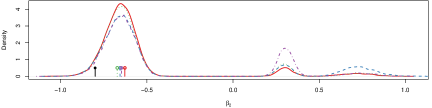
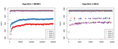
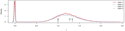
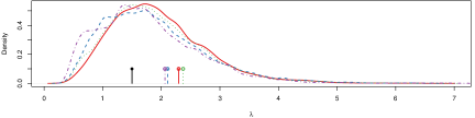
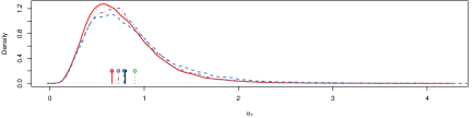
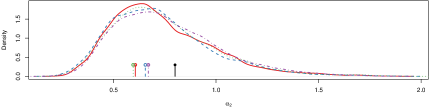
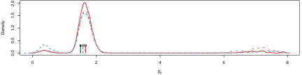
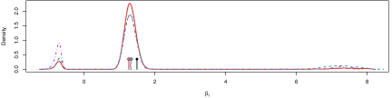
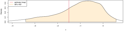
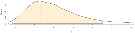
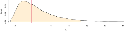
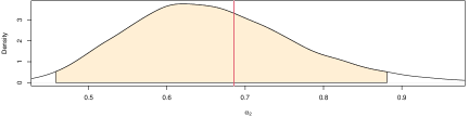
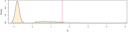
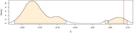
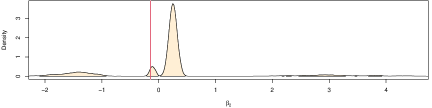
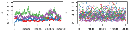
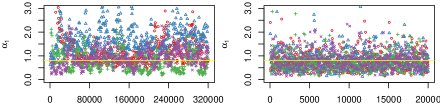
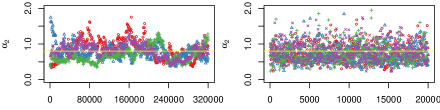
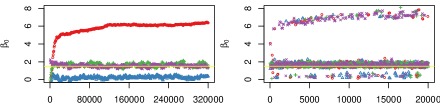
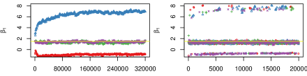
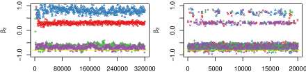
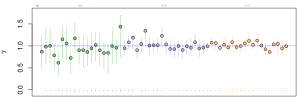
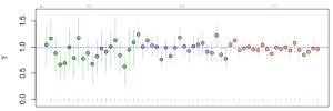
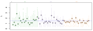
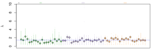
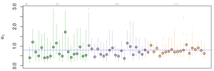
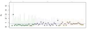
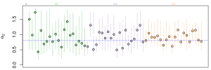
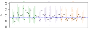
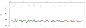
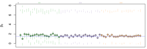
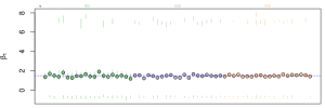
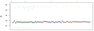
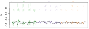
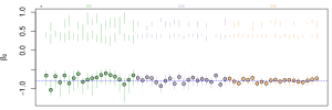
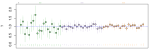
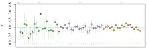
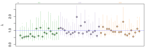
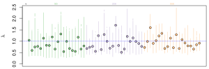
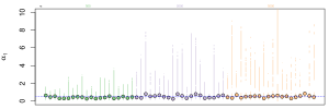
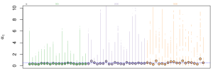
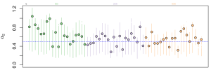
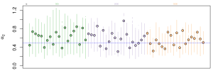
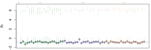
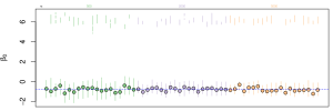
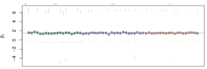
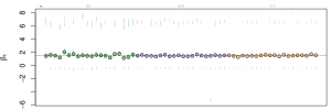
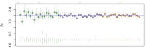
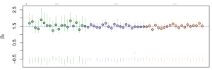
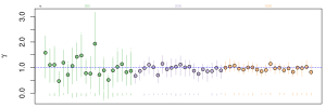
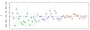
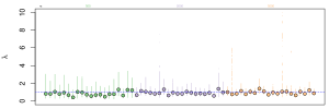
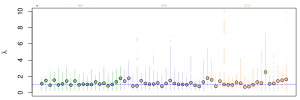
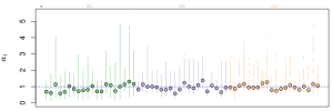
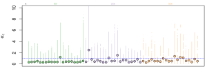
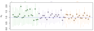
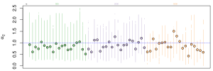
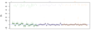
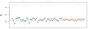
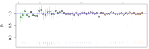
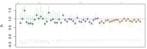
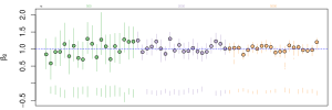
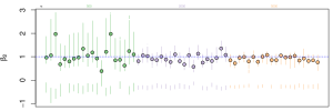
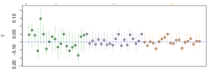
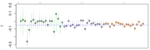
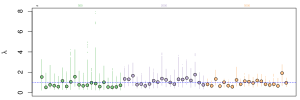
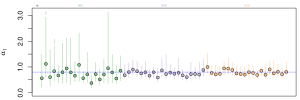
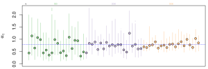
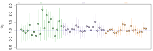
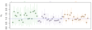
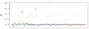
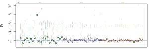
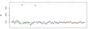
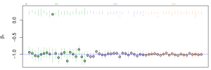
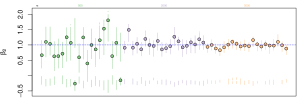
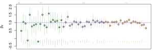
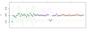
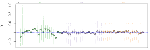
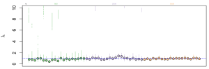
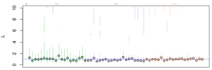
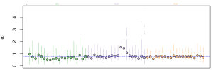
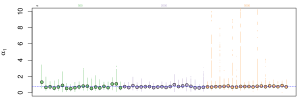
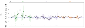
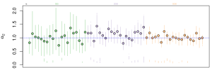
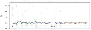
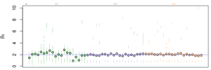
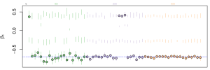
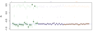
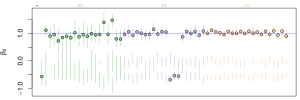
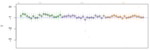
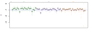
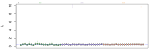
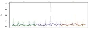
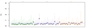
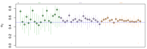
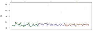
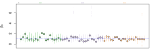
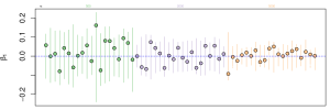
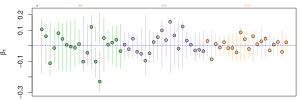
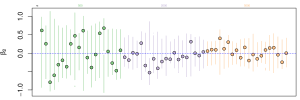
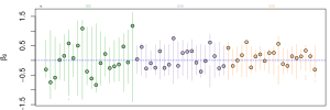
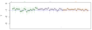
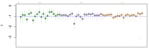
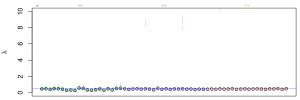
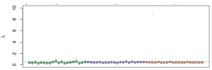
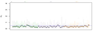
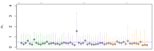
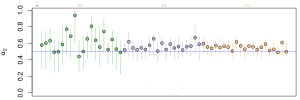
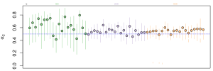
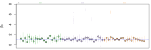
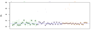
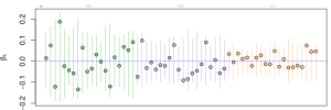
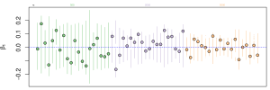
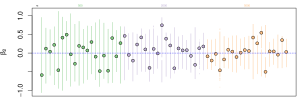
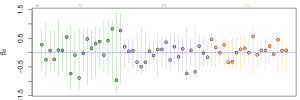
At first we focus on the results for one typical simulated dataset of $n=500$ observations generated from Scenario 1 (see Table 1). Figure 2 shows the resulting estimates of the marginal posterior distribution for 4 different starting values of Algorithm 2, with $C=16$ tempered chains. The multi-modality in the marginal posterior distributions of $\gamma$, $\beta_{0}$, $\beta_{1}$ and $\beta_{2}$ is apparent. For this reason we will be using the Maximum A Posteriori (MAP) estimate as the point estimate of each parameter, i.e., the sampled parameter values which correspond to the iteration with the highest posterior density. These correspond to the coloured vertical lines in Figure 2. We can see that the main mode of the posterior distribution (which corresponds to the one on top of the MAP estimate) contains the true parameter value. For interval estimation we will be using Highest (posterior) Density Intervals (HDI) (which could be discontinuous intervals in general). Observe also that all four runs of our MC3 sampler essentially lead to the same results, thus we can conclude that Algorithm 2 can successfully deal with this multimodal posterior distribution and produce a MCMC sample that converges in relatively small number of iterations in the posterior distribution. This is not the case for Algorithm 1, as shown in Figure 3, where the values of the observed log-likelihood are displayed for four randomly initialized chains. Observe that 2 among 4 chains (in particular chain 1 and chain 2) generated by Algorithm 1 are trapped in a minor mode (see also Appendix D.1).

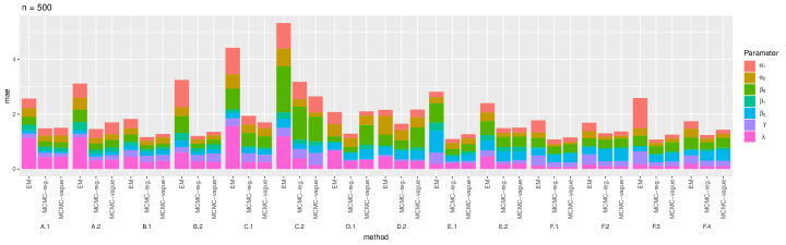
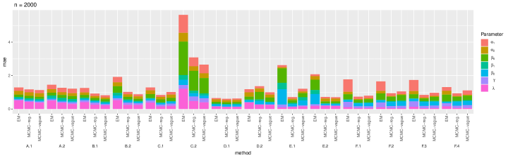
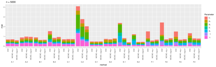
Next, we summarize our findings across all datasets and simulation scenarios. Our method is compared against the EM algorithm (the EM algorithm was used in [44]), based on a small-EM initialization procedure [63] with 45 random starts (the starting values of the EM algorithm were obtained under the same random initialization scheme as in the MCMC sampler; see Appendix A). Figure 4 compares point estimation accuracy for each parameter in terms of the Mean Absolute Error (MAE) between the true value and the point estimate according to each method. The bars represent the cumulative MAE (note that the contribution of each parameter is displayed using distinct colors). It is clear that our MCMC implementation is quite robust for both prior assumptions across all simulation scenarios. More specifically, the MAEs are almost equal for larger sample sizes ($n=2000$ or $n=5000$). In the case of smaller sample size ($n=500$), the regularized prior distribution tends to produce smaller MAEs when compared to the vague prior. Both MCMC implementations outperform the EM algorithm, despite the fact that we have used a rather large number (45) of small runs to initialize the final algorithm. Further summary results per scenario are shown in Figures 11, 12, 13, 14, 15, 16 and 17 in Appendix D.2. In almost all cases, the estimated marginal posterior distributions are multimodal and this mainly affects $\gamma$, $\beta_{0}$, $\beta_{1}$ and $\beta_{2}$. However, it is evident that the MAP estimate of each parameter is close to the “true” value.

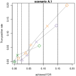
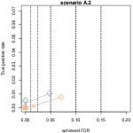
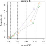
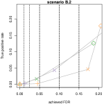
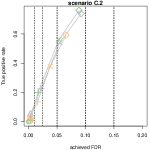
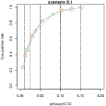
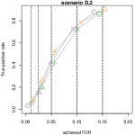
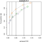
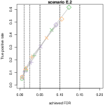
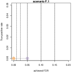
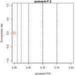
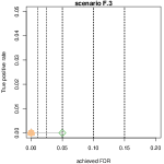
Figure 5 illustrates the achieved FDR of cured subjects, for different levels of target FDR ($\alpha=0.01,0.025,0.05,0.1,0.15$), when applying the decision rule in Equation (13). The $y$ axis corresponds to the detection power (or True Positive Rate) for each value of $\alpha$. Note that in almost every single case, the achieved FDR is smaller than the target FDR (each point is on the left of the corresponding vertical dotted line). This means that our method controls the FDR in the desired level. Most points in the last four scenarios are located to $(0,0)$, meaning that zero cured items are discovered (which is the desired behaviour, since there are no cured items in the sample in these cases). Note that these graphs correspond to the regularized prior distribution. Almost identical results are obtained under the vague prior distribution (results not shown).

Refer to caption
Refer to caption
Refer to caption
Figure 4: The bars display cumulative Mean Absolute Errors (MAE) of parameter estimates for both prior schemes of the proposes MCMC sampler as well as the EM algorithm implementation (according to a small EM initialization scheme based on 45 random starts). MCMC-reg. and MCMC-vague denote the regularized and vague prior distributions, respectively.
Refer to caption Refer to caption Refer to caption
Refer to caption Refer to caption
Figure 5: Achieved False Discovery Rates versus detection power (True Positive Rate) for simulation scenarios 1-16 and various sample sizes, for the regularized prior distribution: 500 (), 2000 (), 5000 (). Distinct point symbols are used to denote the levels of the target FDR $(\alpha)$ for each case: $0.01=\circ$, $0.025=\triangle,0.05=+,0.1=\times,0.15=\diamond$.

5.2 Illustrative example: recidivism

In this section, the proposed methodology is illustrated using a dataset which refers to recidivism for offenders released from prison. The dataset is provided by Iowa Department of Corrections (available for public use in https://data.iowa.gov/; dataset last updated in January 4, 2023 and retrieved in July 6, 2023); it is a set of offenders who left prison (parole/special sentence, work release, or discharge) and reentering the community, after a period of probation supervision. The event of interest is whether the offender was re-incarcerated after probation; every offender was followed for three years (i.e., the censoring time is degenerate at three years).

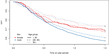
We considered a randomly selected subset of $n=5000$ observations. The following two covariates were taken into account: sex (0: female, 1: male) and age. The recorded times were transformed into two-year periods, as in [44] wherein a previous version of the above dataset was analysed. The confusion matrix of censored items versus sex is shown in Table 2. In order to provide a rough visual summary of the main characteristics of the dataset, the Kaplan-Meier survival function is shown in Figure 6 after grouping age into three (arbitrary) categories: $[18-30)$, $[30,50)$ and larger than $50$. However, in the subsequent analysis, the aforementioned grouping is not taken into account and age is treated as a continuous covariate.

Female Male
Censored 504 2601
Time-to-event 234 1661
Table 2: Recidivism dataset: censored status for females and males.

Before implementing our method we have transformed age so the sample mean and variance equal 0 and 1, respectively. Our results are based on 4 separate runs of Algorithm 2 with different random starting values. For each run we considered $C=16$ tempered chains and a total of $N=100,000$ MCMC cycles. The temperature of each chain was selected according to the following scheme:

$$h_{c}=\frac{1}{(1+\varepsilon)^{c^{d}-1}},\quad c=1,\ldots,C,$$

where $\varepsilon=0.001$ and $d=2.2$. Our reported results are based on discarding the first $30,000$ cycles as burn-in period, and then thinning the chains by keeping every 10th sampled value.

Refer to caption
Figure 6: Kaplan-Meier survival function for the recidivism dataset, after grouping age into three categories.
$\gamma$ $\lambda$ $\alpha_{1}$ $\alpha_{2}$ $\beta_{0}$ $\beta_{1}$ (age) $\beta_{2}$ (sex)
MAP estimate -1.50 3.38 3.81 0.69 1.61 0.09 -0.15
$2.5\%$ quantile -3.58 2.11 1.91 0.47 -1.01 -0.21 -1.82
$25\%$ quantile -1.68 3.04 2.96 0.58 -0.86 -0.18 0.14
$50\%$ quantile -0.95 3.75 3.99 0.65 -0.77 -0.16 0.24
$75\%$ quantile -0.38 4.64 5.55 0.73 -0.62 -0.10 0.31
$97.5\%$ quantile 0.43 7.05 11.10 0.90 2.00 0.09 3.80
Gelman’s diagnostic 1.08 1.01 1.03 1.01 1.06 1.02 1.07
Table 3: Posterior distribution summary for the parameters of the recidivism dataset.

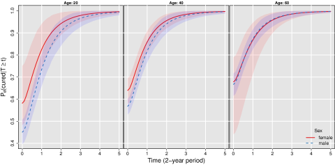
Figure 7 displays the estimated posterior mean of the probability of being cured, conditional on the event that $T\geqslant t$, for females and males, together with the corresponding $95\%$ HDIs. Three different values of the first covariate (age) are displayed, that is, 20, 40 and 60 years old. Clearly, there is a positive effect of age in the mean of cured probability: older offenders are less likely to commit another crime when compared to younger offenders. Moreover, the posterior mean of cure probability is larger for women in smaller values of age. However, as the offender grows older (60 years) the probability of being cured is similar between men and women.

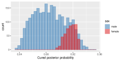
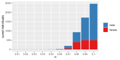
The estimated cured posterior probabilities among the 3105 censored offenders is shown in Figure 8.(a). The corresponding number of cured subjects in the sample is shown in Figure 8.(b), when controlling the FDR at various levels. We see that zero cured subjects are inferred when the target FDR $(\alpha)$ is lower than $0.05$. When $\alpha\in\{0.05,0.06,0.07,0.08,0.09,0.10\}$ the corresponding number of inferred cured items is equal to $2,23,191,932,1722,2465$, respectively.

The MAP estimate of each parameter is reported in Table 3 along with the estimated quantiles. The potential scale reduction factor of the Gelman and Rubin’s convergence diagnostic [64] is smaller than 1.1 for all parameters, thus, it does not spot any convergence issues. See also Figure 9 for the corresponding HDIs. Note that 0 is not included in the HDIs for $\beta_{1}$ and $\beta_{2}$, albeit both parameters exhibit multi-modality.

Refer to caption
Figure 7: Recidivism dataset: estimate of the posterior mean of cured probability for three values of age: 20, 40 and 60. The shaded regions correspond to (pointwise) $95\%$ HDIs.
Refer to caption Refer to caption
(a) (b)
Figure 8: Recidivism dataset. (a) histogram of cured posterior probabilities $\widehat{\mathrm{P}}(I_{j}=0|\boldsymbol{\Delta},\boldsymbol{y},\boldsymbol{x})$ for $j\in\boldsymbol{\Delta}_{0}$ and (b) inferred number of cured individuals when controlling the FDR at level $\alpha$, for the regularized prior distribution.
Refer to caption
Refer to caption
Refer to caption
Refer to caption
Refer to caption
Refer to caption
Refer to caption
Figure 9: Recidivism dataset: kernel density estimates of marginal posterior distributions for each parameter. The shaded region corresponds to the $95\%$ HDI and the vertical line denotes the MAP estimate.

6 Concluding remarks

The family of cure models introduced by [44] incorporates many well studied cure models; for example, the mixture cure rate, the promotion time, the negative binomial and the binomial cure models are all special cases for certain values of the parameters. Typically, the likelihood surface as well as the posterior distribution are multimodal, in order to accommodate these alternative models in various parts of the parameter space. As a consequence, inference is rather challenging both from a likelihood as well as a Bayesian perspective. The proposed Bayesian method introduces a state-of-the-art MCMC sampler and deals with the aforementioned issues in an efficient manner.

A natural extension of the current study may be to explore issues regarding, for example, variable selection; within the Bayesian paradigm, this could be achieved by applying stochastic search variable selection techniques [65, 66] or incorporating shrinkage prior distributions [67]. Model adequacy may be another issue that should be checked; this could be addressed under a predictive viewpoint using cross validation [68], posterior predictive $p$-values [69, 70] or Bayesian goodness of fit-testing procedures [71]. Among authors’ future research directions is also the development of an R package, which would implement the proposed methodology.

Declarations

  • Funding: Panagiotis Papastamoulis received funding from the reseach center of Athens University of Economics and Business.

  • Code and data availability: The (R/C++) code as well as the real dataset used in this paper is available online at https://github.com/mqbssppe/Bayesian_cure_rate_model.

  • Conflict of interest: none.

Appendix A Hyperparameters and MCMC sampler details

$a_{\gamma}$ $b_{\gamma}$ $a_{\lambda}$ $b_{\lambda}$ $a_{1}$ $b_{1}$ $a_{2}$ $b_{2}$ $\mu$ $\Sigma$
vague 0.2 0.1 2.001 1 2.001 1 2.001 1 $(0,\ldots,0)^{\top}$ $100\mathrm{I}_{p}$
regularized 1 1 2.1 1.1 2.1 1.1 2.1 1.1 $(0,\ldots,0)^{\top}$ $10\mathrm{I}_{p}$
Table 4: Parameters of the prior distribution.

We have used two sets of hyper-parameters in the prior distribution as seen in Table 4. The “vague” prior distribution corresponds to a case where the prior variance of each parameter is large. On the other hand, the second choice heavily penalizes large (absolute) values of the parameters and can be seen as a regularization prior on the absolute values of each parameter.

In order to select values of the scale parameters of our Metropolis-Hastings and MALA proposals with a reasonable acceptance rate betweeen proposed moves, the MCMC sampler runs for an initial warm-up period at Step 0 of Algorithm 2. During this period, each parameter is adaptively tuned as the MCMC sampler progresses in order to achieve acceptance rates of the proposed updates between pre-specified limits. The final value of each parameter is then selected as the one that will be used in the subsequent main MCMC sampler. More specifically, the scale parameter of the proposal distributions in Equations (15), (18), (20), (16), (22) were tuned in order to achieve acceptance rates of the proposed moves between $15\%-30\%$. The scale parameter ($\tau$) of the MALA proposal in Equation (10) was tuned until an acceptance rate between $40\%-60\%$ is achieved (see also 55).

A total of $C=16$ tempered chains was considered. The temperature of each chain was selected according to the following scheme:

$$h_{c}=\frac{1}{(1+\varepsilon)^{c^{d}-1}},\quad c=1,\ldots,C,$$

where $\varepsilon>0$, and $d>0$. In our simulations the values $\varepsilon=0.02$ and $b=2.3$ were used. The MCMC sampler was run for a total of $N=20000$ MCMC cycles, with each cycle consisting of $m_{1}=10$ MCMC iterations.

Each chain uses randomly selected initial values based on the following distributions (all independent)

$\displaystyle\gamma$ $\displaystyle\sim\mathcal{N}(0,4)$
$\displaystyle\lambda$ $\displaystyle\sim\mathcal{E}(1)$
$\displaystyle\alpha_{1}$ $\displaystyle\sim\mathcal{E}(1)$
$\displaystyle\alpha_{2}$ $\displaystyle\sim\mathcal{E}(1)$
$\displaystyle\beta_{j}$ $\displaystyle\sim\mathcal{N}(0,4),\quad j=0,1,\ldots,p.$

Appendix B Details of MH and MALA updates

B.1 Metropolis-Hastings step

Firstly, we propose to update $\gamma$ using the following normal proposal distribution

$$\tilde{\gamma}\sim\mathcal{N}\left(\gamma,s^{2}_{\gamma}\right).$$ (14)

All remaining parameters are held fixed (as well as the latent variables $I_{1},\ldots,I_{n}$), and hence this move proposes an update of the form

$$\boldsymbol{\theta}=\left(\gamma,\lambda,\alpha_{1},\alpha_{2},\boldsymbol{\beta}\right)\rightarrow\tilde{\boldsymbol{\theta}}=\left(\tilde{\gamma},\lambda,\alpha_{1},\alpha_{2},\boldsymbol{\beta}\right).$$

Because the density of the proposal distribution in (14) is symmetric to $\gamma^{(t-1)}$ and $\tilde{\gamma}$, the Metropolis-Hastings acceptance probability reduces to

$$A_{1,h}\left(\boldsymbol{\theta},\tilde{\boldsymbol{\theta}}\right)=\min\left\{1,\frac{\dot{f}_{h}(\boldsymbol{y}|\boldsymbol{\Delta},\tilde{\boldsymbol{\theta}},\boldsymbol{I},\boldsymbol{x})\dot{\pi}_{h}(\tilde{\gamma})}{\dot{f}_{h}(\boldsymbol{y}|\boldsymbol{\Delta},\boldsymbol{\theta},\boldsymbol{I},\boldsymbol{x})\dot{\pi}_{h}(\gamma)}\right\}.$$ (15)

If the move is accepted we set $\boldsymbol{\theta}=\tilde{\boldsymbol{\theta}}$, otherwise $\boldsymbol{\theta}=\boldsymbol{\theta}$.

Next, we propose to update $\lambda$ using the following log-normal proposal distribution

$$\tilde{\lambda}\sim\mathcal{LN}\left(\log\left(\lambda\right),s^{2}_{\lambda}\right).$$ (16)

All remaining parameters are held fixed (as well as the latent variables $I_{1},\ldots,I_{n}$), and therefore this move proposes an update of the form

$$\boldsymbol{\theta}=\left(\gamma,\lambda,\alpha_{1},\alpha_{2},\boldsymbol{\beta}\right)\rightarrow\tilde{\boldsymbol{\theta}}=\left(\gamma,\tilde{\lambda},\alpha_{1},\alpha_{2},\boldsymbol{\beta}\right).$$

The ratio of the densities of the proposal distribution in (16) is equal to

$$\frac{q(\tilde{\lambda}\rightarrow\lambda)}{q(\lambda\rightarrow\tilde{\lambda})}=\frac{\tilde{\lambda}}{\lambda};$$

hence, the Metropolis-Hastings acceptance probability reduces to

$$A_{2,h}\left(\boldsymbol{\theta},\tilde{\boldsymbol{\theta}}\right)=\min\left\{1,\frac{\dot{f}_{h}(\boldsymbol{y}|\boldsymbol{\Delta},\tilde{\boldsymbol{\theta}},\boldsymbol{I},\boldsymbol{x})\dot{\pi}_{h}(\tilde{\lambda})\tilde{\lambda}}{\dot{f}_{h}(\boldsymbol{y}|\boldsymbol{\Delta},\boldsymbol{\theta},\boldsymbol{I},\boldsymbol{x})\dot{\pi}_{h}(\lambda)\lambda}\right\}.$$ (17)

If the move is accepted, we update $\boldsymbol{\theta}=\tilde{\boldsymbol{\theta}}$, otherwise $\boldsymbol{\theta}$ is held fixed at its current value.

Next, we propose to update $\alpha_{1}$ using the following log-normal proposal distribution

$$\tilde{\alpha}_{1}\sim\mathcal{LN}\left(\log\left(\alpha_{1}\right),s^{2}_{\alpha_{1}}\right).$$ (18)

All remaining parameters are held fixed (as well as the latent variables $I_{1},\ldots,I_{n}$), and this move proposes an update of the form

$$\boldsymbol{\theta}=\left(\gamma,\lambda,\alpha_{1},\alpha_{2},\boldsymbol{\beta}\right)\rightarrow\tilde{\boldsymbol{\theta}}=\left(\gamma,\lambda,\tilde{\alpha}_{1},\alpha_{2},\boldsymbol{\beta}\right).$$

The Metropolis-Hastings acceptance probability reduces to

$$A_{3,h}\left(\boldsymbol{\theta},\tilde{\boldsymbol{\theta}}\right)=\min\left\{1,\frac{\dot{f}_{h}(\boldsymbol{y}|\boldsymbol{\Delta},\tilde{\boldsymbol{\theta}},\boldsymbol{I},\boldsymbol{x})\dot{\pi}_{h}(\tilde{\alpha}_{1})\tilde{\alpha}_{1}}{\dot{f}_{h}(\boldsymbol{y}|\boldsymbol{\Delta},\boldsymbol{\theta},\boldsymbol{I},\boldsymbol{x})\dot{\pi}_{h}(\alpha_{1})\alpha_{1}}\right\}.$$ (19)

If the move is accepted, we update $\boldsymbol{\theta}=\tilde{\boldsymbol{\theta}}$, otherwise $\boldsymbol{\theta}$ is held fixed at its current value.

Next, we propose to update $\alpha_{2}$ using the following log-normal proposal distribution

$$\tilde{\alpha}_{2}\sim\mathcal{LN}\left(\log\left(\alpha_{2}\right),s^{2}_{\alpha_{2}}\right).$$ (20)

Again, all remaining parameters are held fixed (as well as the latent variables $I_{1},\ldots,I_{n}$), and this move proposes an update of the form

$$\boldsymbol{\theta}=\left(\gamma,\lambda,\alpha_{1},\alpha_{2},\boldsymbol{\beta}\right)\rightarrow\tilde{\boldsymbol{\theta}}=\left(\gamma,\lambda,\alpha_{1},\tilde{\alpha}_{2},\boldsymbol{\beta}\right).$$

The Metropolis-Hastings acceptance probability reduces to

$$A_{4,h}\left(\boldsymbol{\theta},\tilde{\boldsymbol{\theta}}\right)=\min\left\{1,\frac{\dot{f}_{h}(\boldsymbol{y}|\boldsymbol{\Delta},\tilde{\boldsymbol{\theta}},\boldsymbol{I},\boldsymbol{x})\dot{\pi}_{h}(\tilde{\alpha}_{2})\tilde{\alpha}_{2}}{\dot{f}_{h}(\boldsymbol{y}|\boldsymbol{\Delta},\boldsymbol{\theta},\boldsymbol{I},\boldsymbol{x})\dot{\pi}_{h}(\alpha_{2})\alpha_{2}}\right\}.$$ (21)

If the move is accepted, we update $\boldsymbol{\theta}=\tilde{\boldsymbol{\theta}}$, otherwise $\boldsymbol{\theta}$ is held fixed at its current value.

The next step of this move is to propose to simultaneously update all regression coefficients $\boldsymbol{\beta}$, using independent normal proposal distributions, that is,

$$\tilde{\boldsymbol{\beta}}\sim\mathcal{N}_{p}\left(\boldsymbol{\beta},\boldsymbol{\nu}\mathcal{I}_{p}\right)$$ (22)

where $\boldsymbol{\nu}=(\tau_{0},\nu_{1},\ldots,\nu_{k})$ denotes a vector of fixed positive numbers corresponding to the variance of the proposal distribution. Because the density of the proposal distribution in (14) is symmetric to $\boldsymbol{\beta}$ and $\tilde{\boldsymbol{\beta}}$, the Metropolis-Hastings acceptance probability reduces to

$$A_{5,h}\left(\boldsymbol{\beta},\tilde{\boldsymbol{\beta}}\right)=\min\left\{1,\frac{\dot{f}_{h}(\boldsymbol{y}|\boldsymbol{\Delta},\tilde{\boldsymbol{\theta}},\boldsymbol{I},\boldsymbol{x})\dot{\pi}_{h}(\tilde{\boldsymbol{\beta}})}{\dot{f}_{h}(\boldsymbol{y}|\boldsymbol{\Delta},\boldsymbol{\theta},\boldsymbol{I},\boldsymbol{x})\dot{\pi}_{h}(\boldsymbol{\beta})}\right\}.$$ (23)

In all previous acceptance probabilities of the proposed moves, the term $\dot{f}_{h}(\boldsymbol{y}|\boldsymbol{\Delta},\boldsymbol{\theta},\boldsymbol{I},\boldsymbol{x})$ is proportional to $\dot{f}_{h}(\boldsymbol{y},\boldsymbol{I}|\boldsymbol{\Delta},\boldsymbol{\theta},\boldsymbol{x})$ defined in Equation (9). Thus, in all cases, the ratio of conditional densities is equal to $\frac{\dot{f}_{h}(\boldsymbol{y}|\boldsymbol{\Delta},\tilde{\boldsymbol{\theta}},\boldsymbol{I},\boldsymbol{x})}{\dot{f}_{h}(\boldsymbol{y}|\boldsymbol{\Delta},\boldsymbol{\theta},\boldsymbol{I},\boldsymbol{x})}=\frac{\dot{f}_{h}(\boldsymbol{y},\boldsymbol{I}|\boldsymbol{\Delta},\tilde{\boldsymbol{\theta}},\boldsymbol{x})}{\dot{f}_{h}(\boldsymbol{y},\boldsymbol{I}|\boldsymbol{\Delta},\boldsymbol{\theta},\boldsymbol{x})}.$

B.2 MALA step

The proposal in (10) is accepted according to the usual Metropolis-Hastings probability, that is,

$\displaystyle A_{6,h}(\boldsymbol{\theta},\tilde{\boldsymbol{\theta}})=\min\left\{1,\frac{\dot{f}_{h}(\boldsymbol{y}|\boldsymbol{\Delta},\tilde{\boldsymbol{\theta}},\boldsymbol{x},\boldsymbol{I})\dot{\pi}_{h}(\tilde{\boldsymbol{\theta}})}{\dot{f}_{h}(\boldsymbol{y}|\boldsymbol{\Delta},\boldsymbol{\theta},\boldsymbol{x},\boldsymbol{I})\dot{\pi}_{h}(\boldsymbol{\theta})}\frac{\mathrm{P}\left(\tilde{\boldsymbol{\theta}}\rightarrow\boldsymbol{\theta}\right)}{\mathrm{P}\left(\boldsymbol{\theta}\rightarrow\tilde{\boldsymbol{\theta}}\right)}\right\},$ (24)

where $\mathrm{P}\left(a\rightarrow b\right)$ denotes the probability density of proposing state $b$ while in $a$. From (10) we have that $\mathrm{P}\left(\boldsymbol{\theta}\rightarrow\tilde{\boldsymbol{\theta}}\right)$ is the density of the

$$\mathcal{N}_{p+4}\left(\boldsymbol{\theta}+\tau\nabla\log\dot{f}_{h}(\boldsymbol{\theta}|\boldsymbol{y},\boldsymbol{x},\boldsymbol{I}),2\tau\mathcal{I}_{p+4}\right)$$

distribution, evaluated at $\tilde{\boldsymbol{\theta}}$. The density of the reverse transition $\left(\tilde{\boldsymbol{\theta}}\rightarrow\boldsymbol{\theta}\right)$ is equal to the density of the distribution

$$\mathcal{N}_{p+4}\left(\tilde{\boldsymbol{\theta}}+\tau\nabla\log\dot{f}_{h}(\tilde{\boldsymbol{\theta}}|\boldsymbol{\Delta},\boldsymbol{y},\boldsymbol{x},\boldsymbol{I}),2\tau\mathcal{I}_{p+4}\right)$$

evaluated at $\boldsymbol{\beta}^{(t)}$.

From the last Equation it is obvious that if a proposed value lies outside the parameter space, the acceptance probability is zero. In such a case the proposed move is immediately rejected. Certain details for computing the the gradient vector of the logarithm of the joint posterior of $\boldsymbol{\theta}$, conditional on $\boldsymbol{I}$ can be found in Appendix C.

Appendix C Partial derivatives of the complete log-likelihood function

For computing the partial derivatives of the complete log-likelihood

$\displaystyle\log(L_{c})=\sum_{i\in\Delta_{1}}\log f_{P}(y_{i};{\boldsymbol{\theta}},{\boldsymbol{x}}_{i})+\sum_{i\in\Delta_{0}}\log p_{0}({\boldsymbol{x}}_{i};{\boldsymbol{\theta}})+\sum_{i\in\Delta_{0}}I_{i}\log\left(\frac{S_{P}(y_{i};{\boldsymbol{\theta}},{\boldsymbol{x}}_{i})}{p_{0}({\boldsymbol{x}}_{i};{\boldsymbol{\theta}})}-1\right),$

we need the partial derivatives of the functions $f_{P}(y_{i};{\boldsymbol{\theta}},{\boldsymbol{x}}_{i}),p_{0}({\boldsymbol{x}}_{i};{\boldsymbol{\theta}})$ and $S_{P}(y_{i};{\boldsymbol{\theta}},{\boldsymbol{x}}_{i})$. Hence, denoting by $f_{P0}(y_{i};{\boldsymbol{\theta}},{\boldsymbol{x}}_{i})=(1+\gamma\vartheta({\boldsymbol{x}}_{i})c^{\gamma\vartheta({\boldsymbol{x}}_{i})}F(y_{i};\alpha_{1},\alpha_{2})^{\lambda})^{-\frac{1}{\gamma}-1}$, we have

$\displaystyle\frac{\partial\log f_{P}(y_{i};{\boldsymbol{\theta}},{\boldsymbol{x}}_{i})}{\partial\lambda}=\lambda^{-1}+\log F(y_{i};\alpha_{1},\alpha_{2})+\frac{\partial\log f_{P0}(y_{i};{\boldsymbol{\theta}},{\boldsymbol{x}}_{i})}{\partial\lambda}$
$\displaystyle\frac{\partial\log f_{P}(y_{i};{\boldsymbol{\theta}},{\boldsymbol{x}}_{i})}{\partial\gamma}=\theta e^{-1}+\frac{\partial\log f_{P0}(y_{i};{\boldsymbol{\theta}},{\boldsymbol{x}}_{i})}{\partial\gamma}$
$\displaystyle\frac{\partial\log f_{P}(y_{i};{\boldsymbol{\theta}},{\boldsymbol{x}}_{i})}{\partial\alpha_{1}}=(\lambda-1)\frac{\partial\log F(y_{i};\alpha_{1},\alpha_{2})}{\partial\alpha_{1}}+\frac{\partial\log f(y_{i};\alpha_{1},\alpha_{2})}{\partial\alpha_{1}}+\frac{\partial\log f_{P0}(y_{i};{\boldsymbol{\theta}},{\boldsymbol{x}}_{i})}{\partial\alpha_{1}}$
$\displaystyle\frac{\partial\log f_{P}(y_{i};{\boldsymbol{\theta}},{\boldsymbol{x}}_{i})}{\partial\alpha_{2}}=(\lambda-1)\frac{\partial\log F(y_{i};\alpha_{1},\alpha_{2})}{\partial\alpha_{2}}+\frac{\partial\log f(y_{i};\alpha_{1},\alpha_{2})}{\partial\alpha_{2}}+\frac{\partial\log f_{P0}(y_{i};{\boldsymbol{\theta}},{\boldsymbol{x}}_{i})}{\partial\alpha_{2}}$
$\displaystyle\frac{\partial\log f_{P}(y_{i};{\boldsymbol{\theta}},{\boldsymbol{x}}_{i})}{\partial\beta_{j}}=\left(\frac{1}{\vartheta({\boldsymbol{x}}_{i})}+\gamma e^{-1}+\frac{\partial\log f_{P0}(y_{i};{\boldsymbol{\theta}},{\boldsymbol{x}}_{i})}{\partial\vartheta({\boldsymbol{x}}_{i})}\right)\exp(\beta_{0}+{\boldsymbol{\beta}}{\boldsymbol{x}}_{i})x_{j}^{I[j>0]}$

with

$\displaystyle\frac{\partial F(y_{i};\alpha_{1},\alpha_{2})}{\partial\alpha_{1}}=\alpha_{2}y_{i}(\alpha_{1}y_{i})^{\alpha_{2}-1}\exp(-(\alpha_{1}y_{i})^{\alpha_{2}}),$
$\displaystyle\frac{\partial F(y_{i};\alpha_{1},\alpha_{2})}{\partial\alpha_{2}}=\log(\alpha_{1}y_{i})(\alpha_{1}y_{i})^{\alpha_{2}}\exp(-(\alpha_{1}y_{i})^{\alpha_{2}}),$
$\displaystyle\frac{\partial f(y_{i};\alpha_{1},\alpha_{2})}{\partial\alpha_{1}}=(\alpha_{1}y_{i})^{\alpha_{2}-1}\alpha_{2}^{2}\exp(-(\alpha_{1}y_{i})^{\alpha_{2}})\left(1-(\alpha_{1}y_{i})^{\alpha_{2}}\right)$
$\displaystyle\frac{\partial f(y_{i};\alpha_{1},\alpha_{2})}{\partial\alpha_{2}}=\frac{1}{y_{i}}\exp(-(\alpha_{1}y_{i})^{\alpha_{2}})(\alpha_{1}y_{i})^{\alpha_{2}}\left(1+\alpha_{2}\log(\alpha_{1}y_{i})-\alpha_{2}(\alpha_{1}y_{i})^{\alpha_{2}}\log(\alpha_{1}y_{i})\right)$

and

$\displaystyle\frac{\partial\log f_{P0}(y_{i};{\boldsymbol{\theta}},{\boldsymbol{x}}_{i})}{\partial\lambda}=\left(-\frac{1}{\gamma}-1\right)\frac{\gamma\vartheta({\boldsymbol{x}}_{i})c^{\gamma\vartheta({\boldsymbol{x}}_{i})}F(y_{i};\alpha_{1},\alpha_{2})^{\lambda}\log F(y_{i};\alpha_{1},\alpha_{2})}{1+\gamma\vartheta({\boldsymbol{x}}_{i})c^{\gamma\vartheta({\boldsymbol{x}}_{i})}F(y_{i};\alpha_{1},\alpha_{2})^{\lambda}}$
$\displaystyle\frac{\partial\log f_{P0}(y_{i};{\boldsymbol{\theta}},{\boldsymbol{x}}_{i})}{\partial\gamma}=\frac{1}{\gamma^{2}}\log(1+\gamma\vartheta({\boldsymbol{x}}_{i})c^{\gamma\vartheta({\boldsymbol{x}}_{i})}F(y_{i};\alpha_{1},\alpha_{2})^{\lambda})$
$\displaystyle~{}~{}~{}~{}~{}~{}~{}~{}~{}~{}~{}~{}~{}~{}+\left(-\frac{1}{\gamma}-1\right)\vartheta({\boldsymbol{x}}_{i})c^{\gamma\vartheta({\boldsymbol{x}}_{i})}F(y_{i};\alpha_{1},\alpha_{2})^{\lambda}\frac{1+\gamma\vartheta({\boldsymbol{x}}_{i})e^{-1}}{1+\gamma\vartheta({\boldsymbol{x}}_{i})c^{\gamma\vartheta({\boldsymbol{x}}_{i})}F(y_{i};\alpha_{1},\alpha_{2})^{\lambda}}$
$\displaystyle\frac{\partial\log f_{P0}(y_{i};{\boldsymbol{\theta}},{\boldsymbol{x}}_{i})}{\partial\alpha_{1}}=\left(-\frac{1}{\gamma}-1\right)\frac{\lambda\gamma\vartheta({\boldsymbol{x}}_{i})c^{\gamma\vartheta({\boldsymbol{x}}_{i})}F(y_{i};\alpha_{1},\alpha_{2})^{\lambda-1}\frac{\partial F(y_{i};\alpha_{1},\alpha_{2})}{\partial\alpha_{1}}}{1+\gamma\vartheta({\boldsymbol{x}}_{i})c^{\gamma\vartheta({\boldsymbol{x}}_{i})}F(y_{i};\alpha_{1},\alpha_{2})^{\lambda}}$
$\displaystyle\frac{\partial\log f_{P0}(y_{i};{\boldsymbol{\theta}},{\boldsymbol{x}}_{i})}{\partial\alpha_{2}}=\left(-\frac{1}{\gamma}-1\right)\frac{\lambda\gamma\vartheta({\boldsymbol{x}}_{i})c^{\gamma\vartheta({\boldsymbol{x}}_{i})}F(y_{i};\alpha_{1},\alpha_{2})^{\lambda-1}\frac{\partial F(y_{i};\alpha_{1},\alpha_{2})}{\partial\alpha_{2}}}{1+\gamma\vartheta({\boldsymbol{x}}_{i})c^{\gamma\vartheta({\boldsymbol{x}}_{i})}F(y_{i};\alpha_{1},\alpha_{2})^{\lambda}}$
$\displaystyle\frac{\partial\log f_{P0}(y_{i};{\boldsymbol{\theta}},{\boldsymbol{x}}_{i})}{\partial\vartheta({\boldsymbol{x}}_{i})}=\left(-\frac{1}{\gamma}-1\right)\gamma c^{\gamma\vartheta({\boldsymbol{x}}_{i})}F(y_{i};\alpha_{1},\alpha_{2})^{\lambda}\frac{1+\gamma\vartheta({\boldsymbol{x}}_{i})e^{-1}}{1+\gamma\vartheta({\boldsymbol{x}}_{i})c^{\gamma\vartheta({\boldsymbol{x}}_{i})}F(y_{i};\alpha_{1},\alpha_{2})^{\lambda}}.$

Moreover, we have

$\displaystyle\frac{\partial\log p_{0}({\boldsymbol{x}}_{i};{\boldsymbol{\theta}})}{\partial\gamma}=\frac{1}{\gamma}\left(\frac{\log(1+\gamma\vartheta({\boldsymbol{x}}_{i})c^{\gamma\vartheta({\boldsymbol{x}}_{i})})}{\gamma}-\vartheta({\boldsymbol{x}}_{i})c^{\gamma\vartheta({\boldsymbol{x}}_{i})}\frac{1+\gamma e^{-1}\vartheta({\boldsymbol{x}}_{i})}{1+\gamma\vartheta({\boldsymbol{x}}_{i})c^{\gamma\vartheta({\boldsymbol{x}}_{i})}}\right)$
$\displaystyle\frac{\partial\log p_{0}({\boldsymbol{x}}_{i};{\boldsymbol{\theta}})}{\partial\beta_{j}}=-c^{\gamma\vartheta({\boldsymbol{x}}_{i})}\frac{1+\gamma\vartheta({\boldsymbol{x}}_{i})e^{-1}}{1+\gamma\vartheta({\boldsymbol{x}}_{i})c^{\gamma\vartheta({\boldsymbol{x}}_{i})}}\exp(\beta_{0}+{\boldsymbol{\beta}}{\boldsymbol{x}}_{i})x_{j}^{I[j>0]}$

and

$\displaystyle\frac{\partial S_{P}(y_{i};{\boldsymbol{\theta}},{\boldsymbol{x}}_{i})}{\partial\gamma}=S_{P}(y_{i};{\boldsymbol{\theta}},{\boldsymbol{x}}_{i})\left(\frac{1}{\gamma^{2}}\log(1+\gamma\vartheta({\boldsymbol{x}}_{i})c^{\gamma\vartheta({\boldsymbol{x}}_{i})}F(y_{i};\alpha_{1},\alpha_{2})^{\lambda})\right.$
$\displaystyle\left.-\frac{F(y_{i};\alpha_{1},\alpha_{2})^{\lambda}\theta({\boldsymbol{x}}_{i})c^{\gamma\vartheta({\boldsymbol{x}}_{i})}}{\gamma}\frac{1+\gamma\theta({\boldsymbol{x}}_{i})e^{-1}}{1+\gamma\vartheta({\boldsymbol{x}}_{i})c^{\gamma\vartheta({\boldsymbol{x}}_{i})}F(y_{i};\alpha_{1},\alpha_{2})^{\lambda}}\right)$
$\displaystyle\frac{\partial S_{P}(y_{i};{\boldsymbol{\theta}},{\boldsymbol{x}}_{i})}{\partial\lambda}=-f_{P0}(y_{i};{\boldsymbol{\theta}},{\boldsymbol{x}}_{i})\vartheta({\boldsymbol{x}}_{i})c^{\gamma\vartheta({\boldsymbol{x}}_{i})}F(y_{i};\alpha_{1},\alpha_{2})^{\lambda}\log(F(y_{i};\alpha_{1},\alpha_{2}))$
$\displaystyle\frac{\partial S_{P}(y_{i};{\boldsymbol{\theta}},{\boldsymbol{x}}_{i})}{\partial\alpha_{1}}=-f_{P0}(y_{i};{\boldsymbol{\theta}},{\boldsymbol{x}}_{i})\vartheta({\boldsymbol{x}}_{i})c^{\gamma\vartheta({\boldsymbol{x}}_{i})}\lambda F(y_{i};\alpha_{1},\alpha_{2})^{\lambda-1}\frac{\partial F(y_{i};\alpha_{1},\alpha_{2})}{\partial\alpha_{1}}$
$\displaystyle\frac{\partial S_{P}(y_{i};{\boldsymbol{\theta}},{\boldsymbol{x}}_{i})}{\partial\alpha_{2}}=-f_{P0}(y_{i};{\boldsymbol{\theta}},{\boldsymbol{x}}_{i})\vartheta({\boldsymbol{x}}_{i})c^{\gamma\vartheta({\boldsymbol{x}}_{i})}\lambda F(y_{i};\alpha_{1},\alpha_{2})^{\lambda-1}\frac{\partial F(y_{i};\alpha_{1},\alpha_{2})}{\partial\alpha_{2}}$
$\displaystyle\frac{\partial S_{P}(y_{i};{\boldsymbol{\theta}},{\boldsymbol{x}}_{i})}{\partial\beta_{j}}=-f_{P0}(y_{i};{\boldsymbol{\theta}},{\boldsymbol{x}}_{i})c^{\gamma\vartheta({\boldsymbol{x}}_{i})}F(y_{i};\alpha_{1},\alpha_{2})^{\lambda}(1+\gamma\vartheta({\boldsymbol{x}}_{i})e^{-1})\exp(\beta_{0}+{\boldsymbol{\beta}}{\boldsymbol{x}}_{i})x_{j}^{I[j>0]}.$

Appendix D Further simulation results

D.1 Comparison of Algorithms 1 and 2 on a single simulated dataset

Refer to caption
Refer to caption
Refer to caption
Refer to caption
Refer to caption
Refer to caption
Refer to caption
Figure 10: Thinned MCMC outputs for four randomly initialized chains according to Algorithm 1 (left) and Algorithm 2 (right). The horizontal yellow line indicates the values used to generate the dataset.

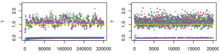
In this section, we provide additional insights to the single synthetic dataset presented in Section 5.1. In order to highlight the benefits of the parallel tempering sampling scheme we compare long runs of Algorithm 1 with shorter runs of parallel tempered chains in Algorithm 2. Recall that the results presented in Figure 2 are based on $N=20000$ cycles of Algorithm 2 with $C=16$ tempered chains. Hence, a total of $m=16\times 20000=320000$ MCMC iterations were considered to Algorithm 1. Each Algorithm ran 4 times from different random starting values.

The corresponding traces of sampled parameter values are displayed in Figure 10 (see for example the generated values of $\gamma$ and $\beta_{0}$). In such cases it is quite challenging to properly explore the posterior surface, since the simulated MCMC sample may be trapped in a local mode. In Figure 10 it is clearly seen that the MC3 implementation (using $C=16$ heated chains) in Algorithm 2 enables the generated parameter values consecutively alternating between the main and the minor ones (this behaviour is vividly illustrated particularly for $\gamma$ and $\beta_{0}$), therefore, the chains are able to freely explore the posterior distribution and avoid getting trapped to the minor mode(s).

D.2 Additional simulation study results

This section contains supplementary Figures 11, 12, 13, 14, 15, 16 and 17, discussed in Section 5.1.

Refer to caption Refer to caption
scenario A.1 scenario A.2
Figure 11: Point estimates (MAP) with $95\%$ Highest Density Intervals for our simulated datasets. Different colour indicate levels of sample size: 500 (), 2000 (), 5000 (). The horizontal line indicates the true value (see Scenarios A1 and A2 in Table 1).
Refer to caption Refer to caption
scenario B.1 scenario B.2
Figure 12: Point estimates (MAP) with $95\%$ Highest Density Intervals for our simulated datasets. Different colour indicate levels of sample size: 500 (), 2000 (), 5000 (). The horizontal line indicates the true value (see Scenarios B1 and B2 in Table 1).
Refer to caption Refer to caption
scenario C.1 scenario C.2
Figure 13: Point estimates (MAP) with $95\%$ Highest Density Intervals for our simulated datasets. Different colour indicate levels of sample size: 500 (), 2000 (), 5000 (). The horizontal line indicates the true value (see Scenarios C1 and C2 in Table 1).
Refer to caption Refer to caption
scenario D.1 scenario D.2
Figure 14: Point estimates (MAP) with $95\%$ Highest Density Intervals for our simulated datasets. Different colour indicate levels of sample size: 500 (), 2000 (), 5000 (). The horizontal line indicates the true value (see Scenarios D1 and D2 in Table 1).
Refer to caption Refer to caption
scenario E.1 scenario E.2
Figure 15: Point estimates (MAP) with $99\%$ Highest Density Intervals for our simulated datasets. Different colour indicate levels of sample size: 500 (), 2000 (), 5000 (). The horizontal line indicates the true value (see Scenarios E1 and E2 in Table 1).
Refer to caption Refer to caption
scenario F.1 scenario F.2
Figure 16: Point estimates (MAP) with $95\%$ Highest Density Intervals for our simulated datasets. Different colour indicate levels of sample size: 500 (), 2000 (), 5000 (). The horizontal line indicates the true value (see Scenarios F1 and F2 in Table 1).
Refer to caption Refer to caption
scenario F.3 scenario F.4
Figure 17: Point estimates (MAP) with $95\%$ Highest Density Intervals for our simulated datasets. Different colour indicate levels of sample size: 500 (), 2000 (), 5000 (). The horizontal line indicates the true value (see Scenarios F3 and F4 in Table 1).

References

  • \bibcommenthead
  • Maller and Zhou [1996] Maller, R.A., Zhou, X.: Survival Analysis with Long-term Survivors. John Wiley & Sons, New York (1996)
  • Peng and Yu [2021] Peng, Y., Yu, B.: Cure Models: Methods, Applications, and Implementation. Chapman and Hall/CRC, New York (2021)
  • Peng and Taylor [2014] Peng, Y., Taylor, J.M.: Cure models. In: Klein, J., Houwelingen, H., Ibrahim, J.G., Scheike, T.H. (eds.) Handbook of Survival Analysis, pp. 113–134. Chapman & Hall,  Boca Raton (2014). Chap. 6
  • Amico and Van Keilegom [2018] Amico, M., Van Keilegom, I.: Cure models in survival analysis. Annual Review of Statistics and its Application 5(1), 311–342 (2018)
  • Rocha et al. [2017] Rocha, R., Nadarajah, S., Tomazella, V., Louzada, F.: A new class of defective models based on the Marshall–Olkin family of distributions for cure rate modeling. Computational Statistics & Data Analysis 107, 48–63 (2017)
  • Schmidt and Witte [1988] Schmidt, P., Witte, A.D.: Predicting Recidivism Using Survival Models. Springer, New York (1988)
  • Peláez et al. [2022] Peláez, R., Van Keilegom, I., Cao, R., Vilar, J.: Probability of default estimation in credit risk using mixture cure models. Technical report, Universidade da Coruña (2022)
  • Yamaguchi [1992] Yamaguchi, K.: Accelerated failure-time regression models with a regression model of surviving fraction: an application to the analysis of permanent employment in Japan. Journal of the American Statistical Association 87(418), 284–292 (1992)
  • Yamaguchi [2003] Yamaguchi, K.: Accelerated failure–time mover–stayer regression models for the analysis of last–episode data. Sociological Methodology 33(1), 81–110 (2003)
  • Kalamatianou and McClean [2003] Kalamatianou, A.G., McClean, S.: The perpetual student: modeling duration of undergraduate studies based on lifetime-type educational data. Lifetime Data Analysis 9(4), 311–330 (2003)
  • Boag [1948a] Boag, J.W.: The presentation and analysis of the results of radiotherapy. Part I. The British Journal of Radiology 21(243), 128–138 (1948)
  • Boag [1948b] Boag, J.W.: The presentation and analysis of the results of radiotherapy. Part II. The British Journal of Radiology 21(244), 189–203 (1948)
  • Boag [1949] Boag, J.W.: Maximum likelihood estimates of the proportion of patients cured by cancer therapy. Journal of the Royal Statistical Society: Series B 11(1), 15–53 (1949)
  • Yakovlev [1994] Yakovlev, A.Y.: Letters to the editor: Parametric versus non-parametric methods for estimating cure rates based on censored survival data. Statistics in Medicine 13(9), 983–986 (1994)
  • Yakovlev et al. [1993] Yakovlev, A.Y., Asselain, B., Bardou, V., Fourquet, A., Hoang, T., Rochefediere, A., Tsodikov, A.: A simple stochastic model of tumor recurrence and its application to data on premenopausal breast cancer. Biometrie et Analyse de Donnees Spatio-temporelles 12, 66–82 (1993)
  • Hoang et al. [1996] Hoang, T., Tsodikov, A., Asselain, B., Yakolev, A.: A parametric analysis of tumor recurrence data. Journal of Biological Systems 4(03), 391–403 (1996)
  • Greenhouse and Wolfe [1984] Greenhouse, J.B., Wolfe, R.A.: A competing risks derivation of a mixture model for the analysis of survival data. Communications in Statistics-Theory and Methods 13(25), 3133–3154 (1984)
  • Larson and Dinse [1985] Larson, M.G., Dinse, G.E.: A mixture model for the regression analysis of competing risks data. Journal of the Royal Statistical Society: Series C (Applied Statistics) 34(3), 201–211 (1985)
  • Meeker [1987] Meeker, W.Q.: Limited failure population life tests: application to integrated circuit reliability. Technometrics 29(1), 51–65 (1987)
  • Meeker and LuValle [1995] Meeker, W.Q., LuValle, M.J.: An accelerated life test model based on reliability kinetics. Technometrics 37(2), 133–146 (1995)
  • Tsodikov et al. [2003] Tsodikov, A.D., Ibrahim, J., Yakovlev, A.: Estimating cure rates from survival data: an alternative to two-component mixture models. Journal of the American Statistical Association 98(464), 1063–1078 (2003)
  • Cooner et al. [2007] Cooner, F.W., Banerjee, S., Carlin, B.P., Sinha, D.: Flexible cure rate modeling under latent activation schemes. Journal of the American Statistical Association 102(478), 560–572 (2007)
  • Tsodikov [2002] Tsodikov, A.D.: Semi-parametric models of long- and short-term survival: an application to the analysis of breast cancer survival in Utah by age and stage. Statistics in Medicine 21(6), 895–920 (2002)
  • Tsodikov [2003] Tsodikov, A.D.: Semiparametric models: a generalized self-consistency approach. Journal of the Royal Statistical Society: Series B 65(3), 759–774 (2003)
  • Balakrishnan and Milienos [2020] Balakrishnan, N., Milienos, F.S.: On a class of non-linear transformation cure rate models. Biometrical Journal 62(5), 1208–1222 (2020)
  • Yin and Ibrahim [2005] Yin, G., Ibrahim, J.G.: Cure rate models: a unified approach. The Canadian Journal of Statistics 33(4), 559–570 (2005)
  • Taylor and Liu [2007] Taylor, J.M., Liu, N.: Statistical issues involved with extending standard models. In: Nair, V. (ed.) Advances in Statistical Modeling and Inference: Essays in Honor of Kjell A Doksum, pp. 299–311. World Scientific, ??? (2007)
  • Peng and Xu [2012] Peng, Y., Xu, J.: An extended cure model and model selection. Lifetime Data Analysis 18(2), 215–233 (2012)
  • Diao and Yin [2012] Diao, G., Yin, G.: A general transformation class of semiparametric cure rate frailty models. Annals of the Institute of Statistical Mathematics 64(5), 959–989 (2012)
  • Pal and Balakrishnan [2017] Pal, S., Balakrishnan, N.: Expectation maximization algorithm for Box–Cox transformation cure rate model and assessment of model misspecification under Weibull lifetimes. IEEE Journal of Biomedical and Health Informatics 22(3), 926–934 (2017)
  • Wang and Pal [2022] Wang, P., Pal, S.: A two-way flexible generalized gamma transformation cure rate model. Statistics in Medicine 41(13), 2427–2447 (2022)
  • Pal and Roy [2023] Pal, S., Roy, S.: On the parameter estimation of Box-Cox transformation cure model. Statistics in Medicine available online (2023)
  • Gilks et al. [2018] Gilks, W.R., Best, N.G., Tan, K.K.C.: Adaptive rejection Metropolis sampling within Gibbs sampling. Journal of the Royal Statistical Society Series C: Applied Statistics 44(4), 455–472 (2018) https://doi.org/10.2307/2986138 https://academic.oup.com/jrsssc/article-pdf/44/4/455/48749639/jrsssc_44_4_455.pdf
  • Tournoud and Ecochard [2008] Tournoud, M., Ecochard, R.: Promotion time models with time-changing exposure and heterogeneity: application to infectious diseases. Biometrical Journal 50(3), 395–407 (2008)
  • Castro et al. [2009] Castro, M.d., Cancho, V.G., Rodrigues, J.: A Bayesian long-term survival model parametrized in the cured fraction. Biometrical Journal 51(3), 443–455 (2009)
  • Ortega et al. [2012] Ortega, E.M., Cordeiro, G.M., Kattan, M.W.: The negative binomial–beta Weibull regression model to predict the cure of prostate cancer. Journal of Applied Statistics 39(6), 1191–1210 (2012)
  • Cordeiro et al. [2016] Cordeiro, G.M., Cancho, V.G., Ortega, E.M., Barriga, G.D.: A model with long-term survivors: negative binomial Birnbaum-Saunders. Communications in Statistics-Theory and Methods 45(5), 1370–1387 (2016)
  • Rodrigues et al. [2018] Rodrigues, A.S., Calsavara, V.F., Tomazella, V.L.D.: Modeling cure fraction with frailty term in latent risk: a Bayesian approach. arXiv preprint arXiv:1803.08128 (2018)
  • D’Andrea et al. [2018] D’Andrea, A., Rocha, R., Tomazella, V., Louzada, F.: Negative binomial Kumaraswamy-G cure rate regression model. Journal of Risk and Financial Management 11(6), 1–14 (2018)
  • Leão et al. [2021] Leão, J., Bourguignon, M., Saulo, H., Santos-Neto, M., Calsavara, V.: The negative binomial beta prime regression model with cure rate: application with a melanoma dataset. Journal of Statistical Theory and Practice 15(3), 1–21 (2021)
  • Pal [2021] Pal, S.: A simplified stochastic EM algorithm for cure rate model with negative binomial competing risks: an application to breast cancer data. Statistics in Medicine 40(28), 6387–6409 (2021)
  • Zeng et al. [2006] Zeng, D., Yin, G., Ibrahim, J.G.: Semiparametric transformation models for survival data with a cure fraction. Journal of the American Statistical Association 101(474), 670–684 (2006)
  • Koutras and Milienos [2017] Koutras, M.V., Milienos, F.S.: A flexible family of transformation cure rate models. Statistics in Medicine 36(16), 2559–2575 (2017)
  • Milienos [2022] Milienos, F.S.: On a reparameterization of a flexible family of cure models. Statistics in Medicine 41(21), 4091–4111 (2022)
  • Geman and Geman [1984] Geman, S., Geman, D.: Stochastic relaxation, gibbs distributions, and the bayesian restoration of images. IEEE Transactions on Pattern Analysis and Machine Intelligence (6), 721–741 (1984)
  • Roberts and Tweedie [1996] Roberts, G.O., Tweedie, R.L.: Exponential convergence of Langevin distributions and their discrete approximations. Bernoulli 2(4), 341–363 (1996)
  • Altekar et al. [2004] Altekar, G., Dwarkadas, S., Huelsenbeck, J.P., Ronquist, F.: Parallel metropolis coupled markov chain monte carlo for bayesian phylogenetic inference. Bioinformatics 20(3), 407–415 (2004)
  • Papastamoulis and Rattray [2018] Papastamoulis, P., Rattray, M.: A Bayesian model selection approach for identifying differentially expressed transcripts from RNA sequencing data. Journal of the Royal Statistical Society: Series C (Applied Statistics) 67(1), 3–23 (2018)
  • Bernhardt [2016] Bernhardt, P.W.: A flexible cure rate model with dependent censoring and a known cure threshold. Statistics in Medicine 35(25), 4607–4623 (2016)
  • Laska and Meisner [1992] Laska, E.M., Meisner, M.J.: Nonparametric estimation and testing in a cure model. Biometrics 48(4), 1223–1234 (1992)
  • Safari et al. [2021] Safari, W.C., López-de-Ullibarri, I., Jácome, M.A.: A product-limit estimator of the conditional survival function when cure status is partially known. Biometrical Journal 63(5), 984–1005 (2021)
  • Safari et al. [2022] Safari, W.C., López-de-Ullibarri, I., Jácome, M.A.: Nonparametric kernel estimation of the probability of cure in a mixture cure model when the cure status is partially observed. Statistical Methods in Medical Research 31(11), 2164–2188 (2022)
  • Safari et al. [2023] Safari, W.C., López-de-Ullibarri, I., Jácome, M.A.: Latency function estimation under the mixture cure model when the cure status is available. Lifetime Data Analysis, 1–20 (2023)
  • Wu et al. [2014] Wu, Y., Lin, Y., Lu, S.-E., Li, C.-S., Shih, W.J.: Extension of a Cox proportional hazards cure model when cure information is partially known. Biostatistics 15(3), 540–554 (2014)
  • Roberts and Rosenthal [1998] Roberts, G.O., Rosenthal, J.S.: Optimal scaling of discrete approximations to langevin diffusions. Journal of the Royal Statistical Society: Series B (Statistical Methodology) 60(1), 255–268 (1998) https://doi.org/10.1111/1467-9868.00123 https://rss.onlinelibrary.wiley.com/doi/pdf/10.1111/1467-9868.00123
  • Girolami and Calderhead [2011] Girolami, M., Calderhead, B.: Riemann manifold Langevin and Hamiltonian Monte Carlo methods. Journal of the Royal Statistical Society: Series B (Statistical Methodology) 73(2), 123–214 (2011)
  • Geyer [1991] Geyer, C.J.: Markov chain monte carlo maximum likelihood. In: Computing Science and Statistics: Proceedings on the 23rd Symposium on the Interface, pp. 156–163. Interface Foundation of North America, ??? (1991)
  • Geyer and Thompson [1995] Geyer, C.J., Thompson, E.A.: Annealing markov chain monte carlo with applications to ancestral inference. Journal of the American Statistical Association 90(431), 909–920 (1995)
  • Benjamini and Hochberg [1995] Benjamini, Y., Hochberg, Y.: Controlling the false discovery rate: a practical and powerful approach to multiple testing. Journal of the Royal statistical society: series B (Methodological) 57(1), 289–300 (1995)
  • Storey [2003] Storey, J.D.: The positive false discovery rate: a Bayesian interpretation and the q-value. The Annals of Statistics 31(6), 2013–2035 (2003)
  • Müller et al. [2004] Müller, P., Parmigiani, G., Robert, C., Rousseau, J.: Optimal sample size for multiple testing: the case of gene expression microarrays. Journal of the American Statistical Association 99(468), 990–1001 (2004)
  • Müller et al. [2006] Müller, P., Parmigiani, G., Rice, K.: Fdr and bayesian multiple comparisons rules. Johns Hopkins University, Dept. of Biostatistics Working Papers Working Paper 115 (2006)
  • Biernacki et al. [2003] Biernacki, C., Celeux, G., Govaert, G.: Choosing starting values for the em algorithm for getting the highest likelihood in multivariate gaussian mixture models. Computational Statistics & Data Analysis 41(3-4), 561–575 (2003)
  • Gelman and Rubin [1992] Gelman, A., Rubin, D.B.: Inference from iterative simulation using multiple sequences. Statistical Science 7(4), 457–472 (1992)
  • George and McCulloch [1995] George, E.I., McCulloch, R.E.: Stochastic search variable selection. Markov chain Monte Carlo in Practice 68(1), 203–214 (1995)
  • Dellaportas et al. [2002] Dellaportas, P., Forster, J.J., Ntzoufras, I.: On bayesian model and variable selection using mcmc. Statistics and computing 12(1), 27–36 (2002)
  • Polson and Scott [2011] Polson, N.G., Scott, J.G.: Shrink Globally, Act Locally: Sparse Bayesian Regularization and Prediction. In: Bayesian Statistics 9. Oxford University Press, ??? (2011). https://doi.org/10.1093/acprof:oso/9780199694587.003.0017 . https://doi.org/10.1093/acprof:oso/9780199694587.003.0017
  • Gelfand et al. [1992] Gelfand, A.E., Dey, D.K., Chang, H.: Model determination using predictive distributions with implementation via sampling-based methods. Bayesian Statistics 4, 147–167 (1992)
  • Meng [1994] Meng, X.-L.: Posterior predictive $p$-values. The Annals of Statistics 22(3), 1142–1160 (1994) https://doi.org/10.1214/aos/1176325622
  • Gelman [2013] Gelman, A.: Two simple examples for understanding posterior p-values whose distributions are far from uniform. Electronic Journal of Statistics 7(none), 2595–2602 (2013) https://doi.org/10.1214/13-EJS854
  • Gelman [2003] Gelman, A.: A bayesian formulation of exploratory data analysis and goodness-of-fit testing. International Statistical Review 71(2), 369–382 (2003)