Hybrid Zonotope-Based Backward Reachability Analysis for Neural Feedback Systems With Nonlinear System Models

Abstract

The increasing prevalence of neural networks in safety-critical control systems underscores the imperative need for rigorous methods to ensure the reliability and safety of these systems. This work introduces a novel approach employing hybrid zonotopes to compute the over-approximation of backward reachable sets for neural feedback systems with nonlinear system models and general activation functions. Closed-form expressions as hybrid zonotopes are provided for the over-approximated backward reachable sets, and a refinement procedure is proposed to alleviate the potential conservatism of the approximation. Two numerical examples are provided to illustrate the effectiveness of the proposed approach.

I Introduction

The integration of Neural Networks (NNs) in feedback control systems necessitates the development of effective methods to analyze the system’s behavior with robust and reliable performance guarantees. Various methods based on set propagation techniques have been proposed for the reachability analysis of Neural Feedback Systems (NFSs), which are systems with NN controllers in the feedback loop. The safety properties of these systems can be verified by the forward reachability analysis [1, 2, 3, 4, 5, 6, 7, 8] or the backward reachability analysis [9, 10, 11].

The backward reachability problem is to compute a set of states, known as the Backward Reachable Set (BRS), from which the system’s trajectories can reach a specified target region within a finite time horizon. When the target region is chosen as the unsafe set for safety verification problems, the computed BRS will bound the back-propagated trajectories that enter the unsafe set. Although there exist various methods for computing the BRSs of systems without NNs [12, 13], they are not directly applicable to NFSs due to the inherently complex and nonlinear nature of NNs. For isolated ReLU-activated NNs, [9] proposed a method to compute the exact BRS of NNs by representing the NNs as piecewise linear functions via the activation patterns of the ReLU functions. For the NFS with linear system dynamics, a method based on Linear Programming (LP) relaxation was proposed in [14] to over-approximate the BRSs; this method was extended in [10] for NFSs with nonlinear system dynamics by utilizing the over-approximation tool OVERT [15] and a guided partition algorithm. Despite the effectiveness of these LP-based methods, the computed BRSs are usually limited in the form of intervals and tend to be conservative.

Recently, Hybrid Zonotope (HZ) was proposed as a new set representation that generalizes the polytope or constrained zonotope [16]. By including binary variables in the set representation, an HZ is equivalent to a finite union of polytopes, and therefore, can conveniently represent non-convex and disconnected sets with flat faces. HZs have proven advantages for set-based computations in terms of computational efficiency and accuracy [16, 17, 18, 19, 20, 21]. In particular, HZs possess properties that make them well-suited for reachability analysis of NFSs. For example, [7] showed that a Feed-forward Neural Network (FNN) with ReLU activation functions can be exactly represented by an HZ and provided algorithms to compute the exact and approximated forward reachable sets of NFSs; [11] considered NFSs with linear dynamics and presented results for computing their exact BRSs in the form of HZs.

This work aims to compute the HZ representations of the over-approximated BRSs for NFSs where the system model is nonlinear and the controller is an FNN with general activation functions. The contributions of this work are at least twofold: (i) By leveraging over-approximation tools of nonlinear functions, closed-form identities are provided for over-approximating the BRSs of NFS with general nonlinear dynamics and ReLU-activated FNN controllers; (ii) The proposed method is extended to NNs with other commonly used activation functions such as leaky ReLU, tanh, and sigmoid. The remainder of this paper is organized as follows: Section II provides preliminaries on HZ and the problem statement; Section III presents the results for NFSs with nonlinear dynamics and ReLU-activated FNNs; Section IV extends these results to NFSs with general activation functions; two numerical examples are provided in Section V to demonstrate the performance of the proposed method; and finally, the concluding remarks are made in Section VI.

Notation. Vectors and matrices are denoted as bold letters (e.g., $\bm{x}\in\mathbb{R}^{n}$ and $\mathbf{A}\in\mathbb{R}^{n\times n}$). The $i$-th component of a vector $\bm{x}\in\mathbb{R}^{n}$ is denoted by $x_{i}$ with $i\in\{1,\dots,n\}$. For a matrix $\mathbf{A}\in\mathbb{R}^{n\times m}$, $\mathbf{A}[i:j,:]$ denotes the matrix constructed by the $i$-th to $j$-th rows of $\mathbf{A}$. The identity matrix in $\mathbb{R}^{n\times n}$ is denoted as $\bm{I}_{n}$ and $\bm{e}_{i}$ is the $i$-th column of $\bm{I}$. The vectors and matrices whose entries are all 0 (resp. 1) are denoted as $\bm{0}$ (resp. $\bm{1}$). Given sets $\mathcal{X}\subset\mathbb{R}^{n}$, $\mathcal{Z}\subset\mathbb{R}^{m}$ and a matrix $\bm{R}\in\mathbb{R}^{m\times n}$, the Cartesian product of $\mathcal{X}$ and $\mathcal{Z}$ is $\mathcal{X}\times\mathcal{Z}=\{(\bm{x},\bm{z})\;|\;\bm{x}\in\mathcal{X},\bm{z}\in\mathcal{Z}\}$, the Minkowski sum of $\mathcal{X}$ and $\mathcal{Z}$ is $\mathcal{X}\oplus\mathcal{Z}=\{\bm{x}+\bm{z}\mid\bm{x}\in\mathcal{X},\bm{z}\in\mathcal{Z}\}$, the generalized intersection of $\mathcal{X}$ and $\mathcal{Z}$ under $\bm{R}$ is $\mathcal{X}\cap_{\bm{R}}\mathcal{Z}=\{\bm{x}\in\mathcal{X}\;|\;\bm{R}\bm{x}\in\mathcal{Z}\}$, and the $k$-ary Cartesian power of $\mathcal{X}$ is $\mathcal{X}^{k}={\mathcal{X}\times\cdots\times\mathcal{X}}$. Given two vectors $\underline{\bm{a}}$, $\overline{\bm{a}}\in\mathbb{R}^{n}$ such that $\underline{\bm{a}}\leq\overline{\bm{a}}$ where $\leq$ is in the element-wise sense, the set $\{\bm{x}\in\mathbb{R}^{n}\mid\underline{\bm{a}}\leq\bm{x}\leq\overline{\bm{a}}\}$ is denoted as $[\![\underline{\bm{a}},\overline{\bm{a}}]\!]$. Given two scalar $\underline{a}$, $\overline{a}\in\mathbb{R}$ such that $\underline{a}\leq\overline{a}$, the interval $\{{x}\in\mathbb{R}\mid\underline{{a}}\leq{x}\leq\overline{{a}}\}$ is denoted as $[\![\underline{{a}},\overline{a}]\!]$.

II Preliminaries & Problem Statement

II-A Hybrid Zonotopes

Definition 1

[16, Definition 3] The set $\mathcal{Z}\subset\mathbb{R}^{n}$ is a hybrid zonotope if there exist $\mathbf{c}\in\mathbb{R}^{n}$, $\mathbf{G}^{c}\in\mathbb{R}^{n\times n_{g}}$, $\mathbf{G}^{b}\in\mathbb{R}^{n\times n_{b}}$, $\mathbf{A}^{c}\in\mathbb{R}^{n_{c}\times{n_{g}}}$, $\mathbf{A}^{b}\in\mathbb{R}^{n_{c}\times{n_{b}}}$, $\mathbf{b}\in\mathbb{R}^{n_{c}}$ such that

$$\mathcal{Z}\!=\!\left\{\begin{bmatrix}\mathbf{G}^{c}\!\!&\!\!\mathbf{G}^{b}\end{bmatrix}\begin{bmatrix}\bm{\xi}^{c}\\ \bm{\xi}^{b}\end{bmatrix}+\mathbf{c}\left|\!\!\begin{array}[]{c}{\begin{bmatrix}\bm{\xi}^{c}\\ \bm{\xi}^{b}\end{bmatrix}\in\mathcal{B}_{\infty}^{n_{g}}\times\{-1,1\}^{n_{b}}},\\ {\begin{bmatrix}\mathbf{A}^{c}\!\!&\!\!\mathbf{A}^{b}\end{bmatrix}\begin{bmatrix}\bm{\xi}^{c}\\ \bm{\xi}^{b}\end{bmatrix}=\mathbf{b}}\end{array}\right.\!\!\!\right\}$$

where $\mathcal{B}_{\infty}^{n_{g}}=\left\{\bm{x}\in\mathbb{R}^{n_{g}}\;|\;\|\bm{x}\|_{\infty}\leq 1\right\}$ is the unit hypercube in $\mathbb{R}^{n_{g}}$. The HCG-representation of the hybrid zonotope is given by $\mathcal{Z}=\langle\mathbf{G}^{c},\allowbreak\mathbf{G}^{b},\allowbreak\mathbf{c},\allowbreak\mathbf{A}^{c},\allowbreak\mathbf{A}^{b},\allowbreak\mathbf{b}\rangle$.

Given an HZ $\mathcal{Z}=\langle\mathbf{G}^{c},\allowbreak\mathbf{G}^{b},\allowbreak\mathbf{c},\allowbreak\mathbf{A}^{c},\allowbreak\mathbf{A}^{b},\allowbreak\mathbf{b}\rangle$, the vector $\mathbf{c}$ is called the center, the columns of $\mathbf{G}^{b}$ are called the binary generators, and the columns of $\mathbf{G}^{c}$ are called the continuous generators. The representation complexity of the HZ $\mathcal{Z}$ is determined by the number of continuous generators $n_{g}$, the number of binary generators $n_{b}$, and the number of equality constraints $n_{c}$ [16]. For simplicity, we define the set $\mathcal{B}(\mathbf{A}^{c},\mathbf{A}^{b},\mathbf{b})\triangleq\{(\bm{\xi}^{c},\bm{\xi}^{b})\in\mathcal{B}^{n_{g}}_{\infty}\times\{-1,1\}^{n_{b}}\;|\;\mathbf{A}^{c}\bm{\xi}^{c}+\mathbf{A}^{b}\bm{\xi}^{b}=\mathbf{b}\}$. An HZ with $n_{b}$ binary generators is equivalent to the union of $2^{n_{b}}$ constrained zonotopes [16, Theorem 5]. Identities are provided to compute the linear map and generalized intersection [16, Proposition 7], the union operation [17, Proposition 1], and the Cartesian product of HZs [18, Proposition 3.2.5].

II-B Problem Statement

Consider the following discrete-time nonlinear system:

$$\bm{x}{(t+1)}=\bm{f}(\bm{x}(t),\bm{u}(t))$$ (1)

where $\bm{x}(t)\in\mathbb{R}^{n},\;\bm{u}(t)\in\mathbb{R}^{m}$ are the state and the control input, respectively. We assume $\bm{x}\in\mathcal{X}$ and $\bm{u}\in\mathcal{U}\triangleq[\![\underline{\bm{u}},\overline{\bm{u}}]\!]$, where $\mathcal{X}\subset\mathbb{R}^{n}$ is called the state set and $\mathcal{U}\subset\mathbb{R}^{m}$ is called the input set. The control input $\bm{u}$ is given as

$$\bm{u}(t)=\bm{\pi}(\bm{x}(t))$$ (2)

where $\pi$ is an $\ell$-layer FNN. The $k$-th layer weight matrix and the bias vector of $\pi$ are denoted as $\bm{W}^{(k-1)}$ and $\bm{v}^{(k-1)}$, respectively, where $k=1,\dots,\ell$. Denote $\bm{x}^{(k)}$ as the neurons of the $k$-th layer and $n_{k}$ as the dimension of $\bm{x}^{(k)}$. Then, for $k=1,\dots,\ell-1$,

$$\bm{x}^{(k)}=\bm{\phi}(\bm{W}^{(k-1)}\bm{x}^{(k-1)}+\bm{v}^{(k-1)})$$ (3)

where $\bm{x}^{(0)}=\bm{x}(t)$ and $\bm{\phi}$ is the vector-valued activation function constructed by component-wise repetition of the activation function $\sigma(\cdot)$, i.e., $\bm{\phi}(\bm{x})\triangleq[\sigma(x_{1})\;\cdots\;\sigma(x_{n})]^{\top}.$ In the last layer, only the linear map is applied, i.e., $\bm{\pi}(\bm{x}(t))=\bm{x}^{(\ell)}=\bm{W}^{(\ell-1)}\bm{x}^{(\ell-1)}+\bm{v}^{(\ell-1)}.$ The activation function considered in this work is not restricted to ReLU; see Section IV for more discussion. In the following, we assume the FNN controller satisfies $\bm{\pi}(\bm{x})\in\mathcal{U}$, $\forall\bm{x}\in\mathcal{X}$; this assumption is not restrictive since the output of any FNN can be saturated into a given range by adding two additional layers with ReLU activation functions [3, 11].

The NFS consisting of system (1) and the controller (2) is a closed-loop system denoted as:

$$\bm{x}{(t+1)}=\bm{f}_{cl}(\bm{x}(t))\triangleq\bm{f}(\bm{x}(t),\bm{\pi}(\bm{x}(t))).$$ (4)

Given a target set $\mathcal{T}\subset\mathcal{X}$ for the system (4), the set of states that can be mapped into the target set $\mathcal{T}$ by (4) in exactly $T$ steps is defined as the $T$-step BRS and denoted as $\mathcal{P}_{T}(\mathcal{T})\triangleq\{\bm{x}(0)\in\mathcal{X}\mid x(t)=\bm{f}_{cl}(\bm{x}(t-1)),x(T)\in\mathcal{T},t=1,2,\dots,T\}.$ For simplicity, the one-step BRS is also denoted as $\mathcal{P}(\mathcal{T})$, i.e., $\mathcal{P}(\mathcal{T})=\mathcal{P}_{1}(\mathcal{T})$. In this work, we assume the state set $\mathcal{X}$, the input set $\mathcal{U}$, the target set $\mathcal{T}$, and the set that over-approximates the nonlinear dynamics $\bm{f}$ are all represented as HZs; this assumption enables us to handle sets and system dynamics using a unified HZ-based approach.

The following problem will be investigated in this work: Given a target set $\mathcal{T}\subset\mathcal{X}$ represented as an HZ and a time horizon $T\in\mathbb{Z}_{>0}$, compute the over-approximation of BRS $\mathcal{P}_{t}(\mathcal{T})$ of the neural feedback system (4), for $t=1,2,\dots,T$.

Compared with our previous result [11] that computes the exact BRS for NFSs consisting of linear dynamics and ReLU-activated FNN controllers, this work considers NFSs consisting of general nonlinear dynamics and FNNs with general activation functions, and therefore, only over-approximated BRSs are computed.

III Backward Reachability Analysis of ReLU Activated Neural Feedback Systems

Our proposed method includes three main steps: (i) compute an HZ envelope of the nonlinear function $\bm{f}$; (ii) find an HZ graph representation of the input-output relationship of the FNN control policy $\bm{\pi}$; (iii) calculate the one-step over-approximated BRS in closed form, and refine the set when necessary. In this section, we assume the controller $\bm{u}$ shown in (2) is an FNN $\bm{\pi}$ with ReLU activation functions across all the layers, i.e., $\sigma(x)=ReLU(x)=\max(x,0)$; this assumption will be relaxed in the next section.

III-A Envelope of Nonlinear Functions

For NFSs with linear dynamics and ReLU activation functions, HZ-based methods have been proposed to compute both the exact forward reachable sets and the exact backward reachable sets [7, 11, 19]. However, since HZs can only represent sets with flat faces (i.e., unions of polytopes), these exact analysis methods are inapplicable to the case of general nonlinear dynamics shown in (4). As the first step towards computing the over-approximated BRS of the system (4), we will find an envelope of the nonlinear function $\bm{f}$.

We denote the graph set of a given function $\bm{f}$ over the domain $\mathcal{X}\times\mathcal{U}$ as $\mathcal{G}_{f}(\mathcal{X},\mathcal{U})\triangleq\{[\bm{x}^{\top}\ \bm{u}^{\top}\ \bm{y}^{\top}]^{\top}\;|\;\bm{y}=\bm{f}(\bm{x},\bm{u}),\bm{x}\in\mathcal{X},\bm{u}\in\mathcal{U}\}$. Since the exact representation of the graph set $\mathcal{G}_{f}(\mathcal{X},\mathcal{U})$ is difficult to find, we will compute an HZ-represented over-approximation of $\mathcal{G}_{f}(\mathcal{X},\mathcal{U})$, denoted as $\overline{\mathcal{H}}_{f}(\mathcal{X},\mathcal{U})$, such that $\overline{\mathcal{H}}_{f}(\mathcal{X},\mathcal{U})\supseteq\mathcal{G}_{f}(\mathcal{X},\mathcal{U})$. The envelope of a nonlinear function over a given domain can be found using off-the-shelf methods [22, 23, 24]. In this work, we make use of two approximation tools, namely Special Ordered Set (SOS) [25] and OVERT [15], mainly because the envelopes obtained by these two methods are easy to compute and can be readily incorporated with the HZ-based set computations.

The over-approximation method based on SOS was originally developed for solving nonlinear and nonconvex optimization problems [25]. In recent work, SOS approximations were utilized to compute the forward reachable set of nonlinear dynamical systems [20]. The SOS approximation $\mathcal{S}$ of a scalar-valued function was defined in [20, Definition 3], while the identity that converts $\mathcal{S}$ into an HZ was provided in [20, Theoem 4]. The maximum SOS approximation error $\bm{\delta}$ for some common nonlinear functions was provided in [24]. Given an SOS approximation $\mathcal{H}_{SOS}$ as an HZ and the maximum approximation error $\bm{\delta}$, an envelop of the function $\bm{f}$ can be given as an HZ $\overline{\mathcal{H}}_{f}(\mathcal{X},\mathcal{U})\triangleq\mathcal{H}_{SOS}\oplus\mathcal{E}$, where $\mathcal{E}=\langle\text{diag}([\bm{0}^{\top}\ \bm{\delta}^{\top}]),\bm{0}\rangle$ is the error zonotope. For nonlinear functions with multidimensional inputs, decomposition techniques can be applied to avoid the exponential complexity of SOS approximations [24].

For the OVERT method, a nonlinear function $\bm{f}$ with multidimensional inputs and outputs will be decomposed into multiple elementary functions $e(\cdot)$ with single inputs and single outputs by the functional rewriting technique, and then over-approximations of the element functions will be constructed using a set of optimally chosen piecewise linear upper and lower bounds [15]. In this work, we assume that the number of breakpoints of the piecewise linear upper and lower bounds, denoted as $N$ ($N\geq 3$), are the same and only optimize the breakpoints along one of the piecewise linear bounds using OVERT. Denote the set of breakpoints for the piecewise linear upper (resp., lower) bound as $\{(x_{i},y_{i}^{ub})\}_{i=1}^{N}$ (resp., $\{(x_{i},y_{i}^{lb})\}_{i=1}^{N}$). Note that the $x$-coordinates of the lower and upper bound are the same. Since the endpoints satisfy $y_{1}^{ub}=y_{1}^{ub}=e(x_{1})$ and $y_{N}^{ub}=y_{N}^{ub}=e(x_{N})$, the set bounded by the piecewise linear upper and lower bounds can be seen as a union of $N-1$ polytopes. Each polytope can be constructed by the breakpoints of the upper and lower bounds, leading to $N-1$ V-rep polytopes that over-approximates the nonlinear element functions. Using [21, Theorem 5], an HZ envelope representing the union of V-rep polytopes can be found.

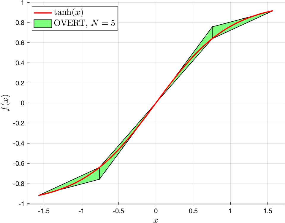
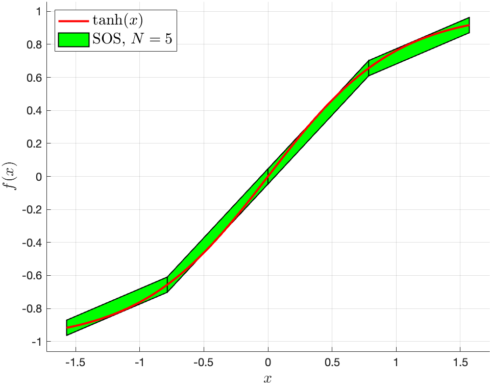
Figure 1: Comparison between OVERT and SOS. Both over-approximate $\tanh(x)$ for $x\in[\![-\pi/2,\pi/2]\!]$ with the union of 4 polytopes.

While both SOS-based and OVERT-based methods can utilize decomposition techniques to generate a tight over-approximation of $\bm{f}$, the resultant HZ envelopes exhibit varying levels of approximation accuracy and set complexity. For example, to compare the set complexity of the resulting HZs, we let the number of breakpoints be $N$ for both the SOS and the OVERT approaches. Then, for any one-dimensional nonlinear elementary function $e(x)$, the complexity of the HZ representations computed by SOS and OVERT is given by $n^{SOS}_{g}=2N+2,\;n^{SOS}_{b}=N-1,\;n^{SOS}_{c}=N+4,n^{OVERT}_{g}=4N-4,\;n^{OVERT}_{b}=N-1,\;n^{OVERT}_{c}=2N.$ It can be observed that the HZ representation based on OVERT approximations tends to have a larger set complexity than the SOS method in terms of more continuous generators and more equality constraints. However, the OVERT method usually leads to more accurate over-approximations than the SOS method. This is because the approximation error $\bm{\delta}$ in the SOS method remains constant across the entire domain, whereas the approximation error in the OVERT method varies based on the distance from the breakpoints. An example of over-approximation of the $\tanh$ function using both methods is shown in Figure 1. Comparisons of the two methods will be further discussed in Section V.

III-B Over-approximation of One-Step BRS

In this subsection, we will compute the closed-form expression of an over-approximation of the one-step BRS, utilizing the HZ envelope of $\bm{f}$ calculated in Section III-A.

In order to incorporate the FNN controller $\bm{\pi}$ into the HZ-based framework, we apply Algorithm 1 in our previous work [11] to compute an HZ-represented graph set of $\bm{\pi}$ over the domain $\mathcal{X}$, denoted as $\mathcal{H}_{\pi}=\langle\mathbf{G}^{c}_{\pi},\allowbreak\mathbf{G}^{b}_{\pi},\allowbreak\mathbf{c}_{\pi},\allowbreak\mathbf{A}^{c}_{\pi},\allowbreak\mathbf{A}^{b}_{\pi},\allowbreak\mathbf{b}_{\pi}\rangle$, i.e., $\mathcal{H}_{\pi}=\mathcal{G}_{\pi}(\mathcal{X})\triangleq\{[\bm{x}^{\top}\ \bm{u}^{\top}]^{\top}\;|\;\bm{u}=\bm{\pi}(\bm{x}),\bm{x}\in\mathcal{X}\}$. Let $\overline{\mathcal{H}}_{f}(\mathcal{X},\mathcal{U})=\langle\mathbf{G}^{c}_{f},\allowbreak\mathbf{G}^{b}_{f},\allowbreak\mathbf{c}_{f},\allowbreak\mathbf{A}^{c}_{f},\allowbreak\mathbf{A}^{b}_{f},\allowbreak\mathbf{b}_{f}\rangle$ be the computed HZ envelope of the nonlinear function $\bm{f}$ over the domain $\mathcal{X}\times\mathcal{U}$ using the approach presented in Section III-A, i.e. $\overline{\mathcal{H}}_{f}(\mathcal{X},\mathcal{U})\supseteq\mathcal{G}_{f}(\mathcal{X},\mathcal{U})$.

With notations above, the following theorem provides the closed-form identities of an over-approximation of the one-step BRS, $\overline{\mathcal{P}}(\mathcal{T})$, with a given target set represented by an HZ.

Theorem 1

Given the state set $\mathcal{X}$, the input set $\mathcal{U}$ and a target set represented by an HZ $\mathcal{T}=\langle\mathbf{G}^{c}_{\tau},\allowbreak\mathbf{G}^{b}_{\tau},\allowbreak\mathbf{c}_{\tau},\allowbreak\mathbf{A}^{c}_{\tau},\allowbreak\mathbf{A}^{b}_{\tau},\allowbreak\mathbf{b}_{\tau}\rangle\subset\mathbb{R}^{n}$, the following HZ is an over-approximated one-step BRS of the NFS (4):

$$\overline{\mathcal{P}}(\mathcal{T})=\langle\mathbf{G}^{c}_{p},\mathbf{G}^{b}_{p},\mathbf{c}_{p},\mathbf{A}^{c}_{p},\mathbf{A}^{b}_{p},\mathbf{b}_{p}\rangle$$ (5)

where $\mathbf{c}_{p}\!=\!\mathbf{c}_{\pi}[1:n,:],\;\mathbf{G}^{c}_{p}\!=\!\begin{bmatrix}\mathbf{G}^{c}_{\pi}[1:n,:]&\bm{0}&\bm{0}\end{bmatrix},\;\mathbf{G}^{b}_{p}=\begin{bmatrix}\mathbf{G}^{b}_{\pi}[1:n,:]&\bm{0}&\bm{0}\end{bmatrix}$ and

$$\mathbf{A}^{c}_{p} \!=\!\begin{bmatrix}\mathbf{A}^{c}_{\pi}\!&\!\bm{0}\!&\!\bm{0}\\ \bm{0}\!&\!\mathbf{A}^{c}_{f}\!&\!\bm{0}\\ \bm{0}\!&\!\bm{0}\!&\!\mathbf{A}^{c}_{\tau}\\ \mathbf{G}^{c}_{\pi}\!&\!-\mathbf{G}^{c}_{f}[1:n+m,:]\!&\!\bm{0}\\ \bm{0}\!&\!\mathbf{G}^{c}_{f}[n+m+1:2n+m,:]\!&\!-\mathbf{G}^{c}_{\tau}\end{bmatrix}\!,$$

$$\mathbf{A}^{b}_{p} \!=\!\begin{bmatrix}\mathbf{A}^{b}_{\pi}\!&\!\bm{0}\!&\!\bm{0}\\ \bm{0}\!&\!\mathbf{A}^{b}_{f}\!&\!\bm{0}\\ \bm{0}\!&\!\bm{0}\!&\!\mathbf{A}^{b}_{\tau}\\ \mathbf{G}^{b}_{\pi}\!&\!-\mathbf{G}^{b}_{f}[1:n+m,:]\!&\!\bm{0}\\ \bm{0}\!&\!\mathbf{G}^{b}_{f}[n+m+1:2n+m,:]\!&\!-\mathbf{G}^{b}_{\tau}\end{bmatrix}\!,$$

$$\mathbf{b}_{p} \!=\!\begin{bmatrix}\mathbf{b}_{\pi}\\ \mathbf{b}_{f}\\ \mathbf{b}_{\tau}\\ \mathbf{c}_{f}[1:n+m,:]-\mathbf{c}_{\pi}\\ \mathbf{c}_{\tau}-\mathbf{c}_{f}[n+m+1:2n+m,:]\end{bmatrix}.$$

Proof:

By the definition of the one-step BRS, we have $\mathcal{P}(\mathcal{T})=\{\bm{x}\in\mathcal{X}\;|\;\bm{f}(\bm{x},\bm{u})\in\mathcal{T},\bm{u}=\bm{\pi}(\bm{x})\}=\{\bm{x}\;|\;\bm{x}\in\mathcal{X},\bm{u}\in\mathcal{U},\bm{u}=\bm{\pi}(\bm{x}),\bm{y}=\bm{f}(\bm{x},\bm{u}),\bm{y}\in\mathcal{T}\}=\{\bm{x}\;|\;[\bm{x}^{\top}\ \bm{u}^{\top}]^{\top}\in\mathcal{H}_{\pi},[\bm{x}^{\top}\ \bm{u}^{\top}\ \bm{y}^{\top}]^{\top}\in\mathcal{G}_{f}(\mathcal{X},\mathcal{U}),\bm{y}\in\mathcal{T}\}.$ Denote $\mathcal{H}_{p}=\{\bm{x}\;|\;[\bm{x}^{\top}\ \bm{u}^{\top}]^{\top}\in\mathcal{H}_{\pi},[\bm{x}^{\top}\ \bm{u}^{\top}\ \bm{y}^{\top}]^{\top}\in\overline{\mathcal{H}}_{f}(\mathcal{X},\mathcal{U}),\bm{y}\in\mathcal{T}\}$. Since $\overline{\mathcal{H}}_{f}(\mathcal{X},\mathcal{U})\supseteq\mathcal{G}_{f}(\mathcal{X},\mathcal{U})$, it’s easy to check that $\mathcal{H}_{p}$ is an over-approximation of the one-step BRS $\mathcal{P}(\mathcal{T})$,i.e., $\mathcal{H}_{p}\supseteq\mathcal{P}(\mathcal{T})$. The remaining of this proof is then to show that $\mathcal{H}_{p}=\overline{P}(\mathcal{T})$.

We will first prove that $\mathcal{H}_{p}\subseteq\overline{P}(\mathcal{T})$. Let $\bm{x}$ be any element of set $\mathcal{H}_{p}$. Then, there exist $\bm{\xi}^{c}_{\pi},\bm{\xi}^{b}_{\pi},\bm{\xi}^{c}_{f},\bm{\xi}^{b}_{f},\bm{\xi}^{c}_{\tau}$ and $\bm{\xi}^{b}_{\tau}$ such that $(\bm{\xi}_{\pi}^{c},\bm{\xi}_{\pi}^{b})\in\mathcal{B}(\mathbf{A}^{c}_{\pi},\mathbf{A}^{b}_{\pi},\mathbf{b}_{\pi})$, $(\bm{\xi}_{f}^{c},\bm{\xi}_{f}^{b})\in\mathcal{B}(\mathbf{A}^{c}_{f},\mathbf{A}^{b}_{f},\mathbf{b}_{f})$, $(\bm{\xi}_{\tau}^{c},\bm{\xi}_{\tau}^{b})\in\mathcal{B}(\mathbf{A}^{c}_{\tau},\mathbf{A}^{b}_{\tau},\mathbf{b}_{\tau})$, and

$$[\bm{x}^{\top}\;\bm{u}^{\top}]^{\top} =\mathbf{G}^{c}_{\pi}\bm{\xi}_{\pi}^{c}+\mathbf{G}^{b}_{\pi}\bm{\xi}^{b}_{\pi}+\mathbf{c}_{\pi},$$ (6a)

$$[\bm{x}^{\top}\;\bm{u}^{\top}\;\bm{y}^{\top}]^{\top} =\mathbf{G}^{c}_{f}\bm{\xi}_{f}^{c}+\mathbf{G}^{b}_{f}\bm{\xi}^{b}_{f}+\mathbf{c}_{f},$$ (6b)

$$\bm{y} =\mathbf{G}^{c}_{\tau}\bm{\xi}_{\tau}^{c}+\mathbf{G}^{b}_{\tau}\bm{\xi}^{b}_{\tau}+\mathbf{c}_{\tau}.$$ (6c)

Therefore, using (6a), we have $\bm{x}=[\bm{I}_{n}\;\bm{0}][\bm{x}^{\top}\;\bm{u}^{\top}]^{\top}=\mathbf{G}^{c}_{\pi}[1:n,:]\bm{\xi}_{\pi}^{c}+\mathbf{G}^{b}_{\pi}[1:n,:]\bm{\xi}^{b}_{\pi}+\mathbf{c}_{\pi}[1:n,:]$. Using (6b), we have $[\bm{x}^{\top}\;\bm{u}^{\top}]^{\top}=[\bm{I}_{n+m}\;\bm{0}][\bm{x}^{\top}\;\bm{u}^{\top}\;\bm{y}^{\top}]^{\top}=\mathbf{G}^{c}_{f}[1:n+m,:]\bm{\xi}_{f}^{c}+\mathbf{G}^{b}_{f}[1:n+m,:]\bm{\xi}^{b}_{f}+\mathbf{c}_{f}[1:n+m,:]$, and $\bm{y}=[\bm{0}\;\bm{I}_{n}][\bm{x}^{\top}\;\bm{y}^{\top}]^{\top}=\mathbf{G}^{c}_{f}[n+m+1:2n+m,:]\bm{\xi}_{f}^{c}+\mathbf{G}^{b}_{f}[n+m+1:2n+m,:]\bm{\xi}^{b}_{f}+\mathbf{c}_{f}[n+m+1:2n+m,:]$. Combining (6a) and $[\bm{x}^{\top}\;\bm{u}^{\top}]^{\top}$ from (6b), we have $\mathbf{G}^{c}_{f}[1:n+m,:]\bm{\xi}_{f}^{c}+\mathbf{G}^{b}_{f}[1:n+m,:]\bm{\xi}^{b}_{f}+\mathbf{c}_{f}[1:n+m,:]=\mathbf{G}^{c}_{\pi}\bm{\xi}_{\pi}^{c}+\mathbf{G}^{b}_{\pi}\bm{\xi}^{b}_{\pi}+\mathbf{c}_{\pi}$. Similarly, by combing (6c) and $\bm{y}$ computed from (6b), we get $\mathbf{G}^{c}_{f}[n+m+1:2n+m,:]\bm{\xi}_{f}^{c}+\mathbf{G}^{b}_{f}[n+m+1:2n+m,:]\bm{\xi}^{b}_{f}+\mathbf{c}_{f}[n+m+1:2n+m,:]=\mathbf{G}^{c}_{\tau}\bm{\xi}_{\tau}^{c}+\mathbf{G}^{b}_{\tau}\bm{\xi}^{b}_{\tau}+\mathbf{c}_{\tau}$. Let $\bm{\xi}^{c}=[(\bm{\xi}^{c}_{\pi})^{\top}\;(\bm{\xi}^{c}_{f})^{\top}\;(\bm{\xi}^{c}_{\tau})^{\top}]^{\top}$ and $\bm{\xi}^{b}=[(\bm{\xi}^{b}_{\pi})^{\top}\;(\bm{\xi}^{b}_{f})^{\top}\;(\bm{\xi}^{b}_{\tau})^{\top}]^{\top}$. Then, it’s easy to check that $\begin{bmatrix}\mathbf{G}^{c}_{\pi}[1\!:\!n,:]\!&\!\bm{0}\!&\!\bm{0}\end{bmatrix}\bm{\xi}^{c}+\begin{bmatrix}\mathbf{G}^{b}_{\pi}[1\!:\!n,:]\!&\!\bm{0}\!&\!\bm{0}\end{bmatrix}\bm{\xi}^{b}+\mathbf{c}_{\pi}[1\!:\!n,:]=\mathbf{G}^{c}_{p}\bm{\xi}^{c}+\mathbf{G}^{b}_{p}\bm{\xi}^{b}+\mathbf{c}_{p}$ and $(\bm{\xi}^{c},\bm{\xi}^{b})\in\mathcal{B}(\mathbf{A}^{c}_{p},\mathbf{A}^{b}_{p},\mathbf{b}_{p})$. Thus, we have $\bm{x}\in\overline{P}(\mathcal{T})$. Since $\bm{x}$ is arbitrary, we get $\mathcal{H}_{p}\subseteq\overline{P}(\mathcal{T})$.

Next, we’ll show that $\mathcal{H}_{p}\supseteq\overline{P}(\mathcal{T})$. Let $\bm{x}\in\overline{P}(\mathcal{T})$. Then, there exist $\bm{\xi}^{c}$ and $\bm{\xi}^{b}$ such that $(\bm{\xi}^{c},\bm{\xi}^{b})\in\mathcal{B}(\mathbf{A}^{c}_{p},\mathbf{A}^{b}_{p},\mathbf{b}_{p})$ and $\bm{x}=\mathbf{G}^{c}_{p}\bm{\xi}^{c}+\mathbf{G}^{b}_{p}\bm{\xi}^{b}+\mathbf{c}_{p}$. Partitioning $\bm{\xi}^{c}$ as $\bm{\xi}^{c}=[(\bm{\xi}^{c}_{\pi})^{\top}\;(\bm{\xi}^{c}_{f})^{\top}\;(\bm{\xi}^{c}_{\tau})^{\top}]^{\top}$ and $\bm{\xi}^{b}$ as $\bm{\xi}^{b}=[(\bm{\xi}^{b}_{\pi})^{\top}\;(\bm{\xi}^{b}_{f})^{\top}\;(\bm{\xi}^{b}_{\tau})^{\top}]^{\top}$, it follows that $(\bm{\xi}_{\pi}^{c},\bm{\xi}_{\pi}^{b})\in\mathcal{B}(\mathbf{A}^{c}_{\pi},\mathbf{A}^{b}_{\pi},\mathbf{b}_{\pi})$, $(\bm{\xi}_{f}^{c},\bm{\xi}_{f}^{b})\in\mathcal{B}(\mathbf{A}^{c}_{f},\mathbf{A}^{b}_{f},\mathbf{b}_{f})$, $(\bm{\xi}_{\tau}^{c},\bm{\xi}_{\tau}^{b})\in\mathcal{B}(\mathbf{A}^{c}_{\tau},\mathbf{A}^{b}_{\tau},\mathbf{b}_{\tau})$ and $\bm{x}=\mathbf{G}^{c}_{\pi}[1:n,:]\bm{\xi}_{\pi}^{c}+\mathbf{G}^{b}_{\pi}[1:n,:]\bm{\xi}^{b}_{\pi}+\mathbf{c}_{\pi}[1:n,:]=\mathbf{G}^{c}_{f}[1:n,:]\bm{\xi}_{f}^{c}+\mathbf{G}^{b}_{f}[1:n,:]\bm{\xi}^{b}_{f}+\mathbf{c}_{f}[1:n,:]$. Choose $\bm{u}=\mathbf{G}^{c}_{\pi}[n+1:n+m,:]\bm{\xi}_{\pi}^{c}+\mathbf{G}^{b}_{\pi}[n+1:n+m,:]\bm{\xi}^{b}_{\pi}+\mathbf{c}_{\pi}[n+1:n+m,:]$ and $\bm{y}=\mathbf{G}^{c}_{f}[n+m+1:2n+m,:]\bm{\xi}_{f}^{c}+\mathbf{G}^{b}_{f}[n+m+1:2n+m,:]\bm{\xi}^{b}_{f}+\mathbf{c}_{f}[n+m+1:2n+m,:]$. Then, we can get $[\bm{x}^{\top}\;\bm{u}^{\top}]^{\top}=\mathbf{G}^{c}_{\pi}\bm{\xi}_{\pi}^{c}+\mathbf{G}^{b}_{\pi}\bm{\xi}^{b}_{\pi}+\mathbf{c}_{\pi}$, $[\bm{x}^{\top}\;\bm{u}^{\top}\;\bm{y}^{\top}]^{\top}=\mathbf{G}^{c}_{f}\bm{\xi}_{f}^{c}+\mathbf{G}^{b}_{f}\bm{\xi}^{b}_{f}+\mathbf{c}_{f}$, and $\bm{y}=\mathbf{G}^{c}_{\tau}\bm{\xi}_{\tau}^{c}+\mathbf{G}^{b}_{\tau}\bm{\xi}^{b}_{\tau}+\mathbf{c}_{\tau}$. Thus, $\bm{x}\in\mathcal{H}_{p}$. Since $\bm{x}$ is arbitrary, $\mathcal{H}_{p}\supseteq\overline{P}(\mathcal{T})$. Therefore, we conclude that $\mathcal{H}_{p}=\overline{P}(\mathcal{T})$. ∎

Theorem 1 can be applied to NFSs with general nonlinear dynamics, but the set $\overline{\mathcal{P}}(\mathcal{T})$ computed may induce redundant equality constraints in the HZ representation. The following result provides a BRS representation of $\overline{\mathcal{P}}(\mathcal{T})$ with less redundant constraints for NFSs with a special class of nonlinear dynamics.

Corollary 1

Consider an NFS (4) where $\bm{f}(\bm{x}(t),\bm{u}(t))=\bm{g}(\bm{x}(t))+\bm{B}_{d}\bm{u}(t)$. Given the state set $\mathcal{X}$, the input set $\mathcal{U}$ and a target set represented by an HZ $\mathcal{T}=\langle\mathbf{G}^{c}_{\tau},\allowbreak\mathbf{G}^{b}_{\tau},\allowbreak\mathbf{c}_{\tau},\allowbreak\mathbf{A}^{c}_{\tau},\allowbreak\mathbf{A}^{b}_{\tau},\allowbreak\mathbf{b}_{\tau}\rangle\subset\mathbb{R}^{n}$, let $\mathcal{H}_{\pi}=\langle\mathbf{G}^{c}_{\pi},\allowbreak\mathbf{G}^{b}_{\pi},\allowbreak\mathbf{c}_{\pi},\allowbreak\mathbf{A}^{c}_{\pi},\allowbreak\mathbf{A}^{b}_{\pi},\allowbreak\mathbf{b}_{\pi}\rangle$ be the computed HZ-based graph set of the FNN $\pi$ over the domain $\mathcal{X}$. Let $\overline{\mathcal{H}}_{g}(\mathcal{X})=\langle\mathbf{G}^{c}_{g},\allowbreak\mathbf{G}^{b}_{g},\allowbreak\mathbf{c}_{g},\allowbreak\mathbf{A}^{c}_{g},\allowbreak\mathbf{A}^{b}_{g},\allowbreak\mathbf{b}_{g}\rangle$ be the computed HZ envelope of the nonlinear function $\bm{g}$ over the domain $\mathcal{X}$. Then, an over-approximated one-step BRS of the NFS can be computed as an HZ given by $\tilde{\mathcal{P}}(\mathcal{T})=\langle\mathbf{G}^{c}_{p},\mathbf{G}^{b}_{p},\mathbf{c}_{p},{\tilde{\mathbf{A}}^{c}_{p}},{\tilde{\mathbf{A}}^{b}_{p}},{\tilde{\mathbf{b}}_{p}}\rangle,$ where $\mathbf{G}^{c}_{p},\mathbf{G}^{b}_{p},\mathbf{c}_{p}$ are the same as in Theorem 1, $\tilde{\mathbf{b}}_{p}=\begin{bmatrix}\mathbf{b}_{\pi}^{\top}&\mathbf{b}_{g}^{\top}&\mathbf{b}_{\tau}^{\top}&\mathbf{b}_{1}^{\top}&\mathbf{b}_{2}^{\top}\end{bmatrix}$, $\tilde{\mathbf{A}}^{c}_{p}=\begin{bmatrix}\operatorname{diag}(\mathbf{A}^{c}_{\pi},\mathbf{A}^{c}_{g},\mathbf{A}^{c}_{\tau})\\ \mathbf{A}_{1}\end{bmatrix}$, $\tilde{\mathbf{A}}^{b}_{p}=\begin{bmatrix}\operatorname{diag}(\mathbf{A}^{b}_{\pi},\mathbf{A}^{b}_{g},\mathbf{A}^{b}_{\tau})\\ \mathbf{A}_{2}\end{bmatrix}$ with $\mathbf{b}_{1}=\mathbf{c}_{g}[1:n,:]-\mathbf{c}_{\pi}[1:n,:]$, $\mathbf{b}_{2}=\mathbf{c}_{\tau}-\bm{B}_{d}\mathbf{c}_{\pi}[n+1:n+m,:]-\mathbf{c}_{g}[n+1:2n,:]$, and

$$\mathbf{A}_{1} \!=\!\begin{bmatrix}\mathbf{G}^{c}_{\pi}[1:n,:]\!&\!-\mathbf{G}^{c}_{g}[1:n,:]\!&\!\bm{0}\\ \bm{B}_{d}\mathbf{G}^{c}_{\pi}[n+1:n+m,:]\!&\!\mathbf{G}^{c}_{g}[n+1:2n,:]\!&\!-\mathbf{G}^{c}_{\tau}\end{bmatrix}\!,$$

$$\mathbf{A}_{2} \!=\!\begin{bmatrix}\mathbf{G}^{b}_{\pi}[1:n,:]\!&\!-\mathbf{G}^{b}_{g}[1:n,:]\!&\!\bm{0}\\ \bm{B}_{d}\mathbf{G}^{b}_{\pi}[n+1:n+m,:]\!&\!\mathbf{G}^{b}_{g}[n+1:2n,:]\!&\!-\mathbf{G}^{b}_{\tau}\!\end{bmatrix}\!.$$

The proof of Corollary 1 follows the same procedures as the proof of Theorem 1, and is thus omitted.

III-C Refinement of Over-approximated Multi-step BRS

Based on the results of the preceding subsections, the $K$-step over-approximations of BRS for (4) can be computed iteratively as follows:

$$\mathcal{P}_{0}(\mathcal{T})=\mathcal{T},\;\mathcal{P}_{t}(\mathcal{T})=\mathcal{P}(\mathcal{P}_{t-1}(\mathcal{T})),\;t=1,\dots,T.$$ (7)

Since Theorem 1 computes $\overline{\mathcal{H}}_{f}(\mathcal{X},\mathcal{U})$ over the entire state-input domain $\mathcal{X}\times\mathcal{U}$, a naive application of (7) based on Theorem 1 may lead to conservative approximations for multi-step computations. In order to mitigate the conservativeness, we introduce a refinement procedure aimed at computing $\overline{\mathcal{H}}_{f}$ within more tightly constrained prior sets, denoted as $\mathcal{X}^{p}\times\mathcal{U}^{p}$ where $p$ stands for “prior”. This refinement procedure employs a recursive approach that utilizes the BRSs obtained from the previous $\overline{\mathcal{H}}_{f}$ to compute the new prior sets.

With the same notations as in Theorem 1, the following lemma provides a closed-form expression of an over-approximation of BRS $\overline{\mathcal{P}}(\mathcal{T})$ over the prior sets $\mathcal{X}^{p}\times\mathcal{U}^{p}$.

Lemma 1

Given the state set $\mathcal{X}$, the input set $\mathcal{U}$, the target set $\mathcal{T}$, and the graph set of $\bm{\pi}$, $\mathcal{H}_{\pi}$, suppose that the prior sets $\mathcal{X}^{p}\times\mathcal{U}^{p}$ satisfies

$$\mathcal{H}_{\pi}\cap_{\begin{bmatrix}\bm{I}_{n}&\bm{0}\end{bmatrix}}\mathcal{P}(\mathcal{T})\subseteq\mathcal{X}^{p}\times\mathcal{U}^{p}\subseteq\mathcal{X}\times\mathcal{U}.$$ (8)

Let $\overline{\mathcal{H}}_{f}(\mathcal{X}^{p},\mathcal{U}^{p})=\langle\mathbf{G}^{c}_{fp},\allowbreak\mathbf{G}^{b}_{fp},\allowbreak\mathbf{c}_{fp},\allowbreak\mathbf{A}^{c}_{fp},\allowbreak\mathbf{A}^{b}_{fp},\allowbreak\mathbf{b}_{fp}\rangle$ be the over-approximated graph set of the nonlinear function $\bm{f}$ over the domain $\mathcal{X}^{p}\times\mathcal{U}^{p}$. Then, the one-step BRS of the NFS (4) can be over-approximated by an HZ whose HCG-representation is the same as (5) by replacing $\langle\mathbf{G}^{c}_{f},\allowbreak\mathbf{G}^{b}_{f},\allowbreak\mathbf{c}_{f},\allowbreak\mathbf{A}^{c}_{f},\allowbreak\mathbf{A}^{b}_{f},\allowbreak\mathbf{b}_{f}\rangle$ with $\langle\mathbf{G}^{c}_{fp},\allowbreak\mathbf{G}^{b}_{fp},\allowbreak\mathbf{c}_{fp},\allowbreak\mathbf{A}^{c}_{fp},\allowbreak\mathbf{A}^{b}_{fp},\allowbreak\mathbf{b}_{fp}\rangle$.

Proof:

From (8), we know that $\mathcal{P}(\mathcal{T})\subseteq\mathcal{X}^{p}\subseteq\mathcal{X}$ and $\mathcal{U}_{\mathcal{T}}\subseteq\mathcal{U}^{p}\subseteq\mathcal{U}$, where $\mathcal{U}_{\mathcal{T}}$ denotes the projection of $\mathcal{H}_{\pi}\cap_{\begin{bmatrix}\bm{I}_{n}&\bm{0}\end{bmatrix}}\mathcal{P}(\mathcal{T})$ onto the $\bm{u}$ space. By the definition of the one-step BRS, we have $\mathcal{P}(\mathcal{T})=\{\bm{x}\in\mathcal{X}\;|\;\bm{f}(\bm{x},\bm{u})\in\mathcal{T},\bm{u}=\bm{\pi}(\bm{x})\}=\{\bm{x}\in\mathcal{X}^{p}\mid\bm{f}(\bm{x},\bm{u})\in\mathcal{T},\bm{u}=\bm{\pi}(\bm{x})\}=\{\bm{x}\;|\;[\bm{x}^{\top}\ \bm{u}^{\top}\ \bm{y}^{\top}]^{\top}\in\mathcal{G}_{f}(\mathcal{X}^{p},\mathcal{U}^{p}),\bm{u}=\bm{\pi}(\bm{x}),\bm{y}\in\mathcal{T}\}=\{\bm{x}\;|\;[\bm{x}^{\top}\ \bm{u}^{\top}]^{\top}\in\mathcal{H}_{\pi}\cap_{\begin{bmatrix}\bm{I}_{n}&\bm{0}\end{bmatrix}}\mathcal{P}(\mathcal{T}),[\bm{x}^{\top}\ \bm{u}^{\top}\ \bm{y}^{\top}]^{\top}\in\mathcal{G}_{f}(\mathcal{X}^{p},\mathcal{U}^{p}),\bm{y}\in\mathcal{T}\}=\{\bm{x}\;|\;[\bm{x}^{\top}\ \bm{u}^{\top}]^{\top}\in\mathcal{H}_{\pi},[\bm{x}^{\top}\ \bm{u}^{\top}\ \bm{y}^{\top}]^{\top}\in\mathcal{G}_{f}(\mathcal{X}^{p},\mathcal{U}^{p}),\bm{y}\in\mathcal{T}\}.$ Then the remaining proof is the same as that of Theorem 1. ∎

Input: State domain $\mathcal{X}$, control input domain $\mathcal{U}$, target set $\mathcal{T}$, nonlinear dynamics $\bm{f}$, neural network controller $\bm{\pi}$, large scalars $\alpha,\beta>0$, time horizon $T$, the number of refinement epochs $n_{r}$.

Output: Refined over-approximations of $t$-step BRSs from $t=1$ to $T$ $\overline{\mathcal{P}}_{1:T}(\mathcal{T})$.

1 Initialization: $\overline{\mathcal{P}}_{0}(\mathcal{T})\leftarrow\mathcal{T}$; $\mathcal{X}^{p}_{1:T}\leftarrow\mathcal{X}$; $\mathcal{U}^{p}_{1:T}\leftarrow\mathcal{U}$;

2

Compute $\mathcal{H}_{\pi}$ with $\alpha$ and $\beta$ ;

  // Alg 1 in [11]

3

4for $r\in\{0,1,\dots,n_{r}$} do

5      

6      for $t\in\{1,2,\dots,T$} do

             Compute $\overline{\mathcal{H}}_{f}(\mathcal{X}^{p}_{t},\mathcal{U}^{p}_{t})$;

              // Section III-A

7            

            $\overline{\mathcal{P}}_{t}(\mathcal{T})\leftarrow\text{Pre}(\overline{\mathcal{P}}_{t-1}(\mathcal{T}),\overline{\mathcal{H}}_{f}(\mathcal{X}^{p}_{t},\mathcal{U}^{p}_{t}),\mathcal{H}_{\pi})$;

              // Over-approximate one-step BRS

8            

9            if $n_{r}==0$ or $r==n_{r}$ then

10                  continue;

11                  

12            

            $\mathcal{X}^{p}_{t}$, $\mathcal{U}^{p}_{t}$ $\leftarrow$ ${GetBox}(\overline{\mathcal{P}}_{t}(\mathcal{T}),\mathcal{H}_{\pi})$;

              // The prior sets for $\mathcal{P}_{t}(\mathcal{T})$.

13            

14      

return $\overline{\mathcal{P}}_{1:T}(\mathcal{T})$

Algorithm 1 BReachNonlin-HZ

Algorithm 1 summarizes the over-approximation of BRS for the closed-loop system (4) with the refinement procedure. The prior sets $\mathcal{X}^{p}\times\mathcal{U}^{p}$ for all the time horizons are initialized as $\mathcal{X}\times\mathcal{U}$ (Line 1) and $\mathcal{H}_{\pi}$ is computed over $\mathcal{X}$ with the large scalars $\alpha$ and $\beta$ by using Algorithm 1 in [11] (Line 1). For each time horizon $t$, we compute the over-approximation of the nonlinear dynamics over the prior set $\mathcal{X}^{p}_{t}$ and $\mathcal{U}^{p}_{t}$ (Line 1) and then the over-approximated one-step BRS $\overline{\mathcal{P}}_{t}(\mathcal{T})$ is computed by Lemma 1 (Line 1). If $n_{r}=0$ or the refinement epoch reaches the maximum number $n_{r}$, the refinement procedure will be skipped and the computed BRSs $\overline{\mathcal{P}}_{1:T}(\mathcal{T})$ for $t=1$ to $T$ will be returned; otherwise, the tighter prior sets are computed based on the over-approximated BRSs and then passed to the next refinement epoch (Line 1). Concretely, in Line 1, the $GetBox$ only shrinks the bounding intervals of $\mathcal{X}\times\mathcal{U}$ over the dimensions contributing to the nonlinearity. Let $\bm{r}=[\bm{x}^{\top}\ \bm{u}^{\top}]^{\top}\in\mathcal{H}_{\pi}$. The shrinking interval of the state contributing to the nonlinearity, denoted as $[\![r_{f}^{lb},r_{f}^{ub}]\!]$, can be obtained by solving two Mixed-Integer Linear Programs (MILPs): $r_{f}^{lb}=\min_{\bm{r}\in\mathcal{H}_{\pi}^{\mathcal{T}}}r_{f}$, $r_{f}^{ub}=\max_{\bm{r}\in\mathcal{H}_{\pi}^{\mathcal{T}}}r_{f}$, where $\mathcal{H}_{\pi}^{\mathcal{T}}=\mathcal{H}_{\pi}\cap_{\begin{bmatrix}\bm{I}_{n}&\bm{0}\end{bmatrix}}\overline{\mathcal{P}}(\mathcal{T})$.

Remark 1

The number of refinement epochs $n_{r}$ in Algorithm 1 represents the trade-off between the set approximation accuracy and the computation efficiency. Specifically, the refinement procedure mitigates the conservativeness of the set approximation but requires computing $\overline{\mathcal{H}}_{f}(\mathcal{X}_{t}^{p},\mathcal{U}_{t}^{p})$ and the bounding hyper-boxes of HZs at each epoch, which introduces extra computation time. Simulation results for different numbers of epochs are given in Section V.

Remark 2

The over-approximated BRSs can be used for the safety verification of NFSs [16, 11]. Consider an HZ initial state set $\mathcal{X}_{0}\subset\mathcal{X}$ and an HZ unsafe region $\mathcal{O}\subset\mathcal{X}$. Suppose that the $t$-step BRS of $\mathcal{O}$ is over-approximated as $\overline{\mathcal{P}}_{t}(\mathcal{O})$ via Algorithm 1 for $t=1,\cdots,T$. Then any trajectory that starts from $\mathcal{X}_{0}$ will not enter into the unsafe region $\mathcal{O}$ within $T$ time steps if all the over-approximated BRSs $\overline{\mathcal{P}}_{1:T}(\mathcal{O})$ have no intersections with the initial set $\mathcal{X}_{0}$. By [16, Proposition 7] and [11, Lemma 1], verifying the emptiness of the intersection of $\mathcal{X}_{0}$ and $\overline{\mathcal{P}}_{t}(\mathcal{O})$ is equivalent to solve an MILP.

IV Neural Feedback System With General Types of Activation Functions

In this section, we extend the results of the preceding section that considers ReLU-activated FNNs to FNNs with more general activation functions. We categorize the activation functions as either piecewise linear or non-piecewise linear. For FNNs with piecewise linear activation functions, their exact graph sets can be constructed, in which case Theorem 1 and Lemma 1 are directly applicable. For FNNs with non-piecewise linear activation functions, their graph sets can be over-approximated by using the methods in Section III-A, based on which the over-approximated BRSs can be computed.

IV-A Piecewise Linear Activation Functions

The graph of piecewise linear activation functions can be exactly represented by a finite union of polytopes that is equivalent to an HZ. For simplicity, we use the Parametric ReLU (PReLU) activation function as an example to show the construction of the graph set.

The PReLU is a parametric activation function defined as

$$\sigma\left(x\right)=\left\{\begin{array}[]{ll}x,&\text{ if }x>0,\\ ax,&\text{ if }x\leq 0.\end{array}\right.$$

Here $a\in\mathbb{R}_{\geq 0}$ is a parameter that is learned along with other neural network parameters [26]. When $a=0$, it becomes the conventional ReLU; when $a$ is a small positive number, it becomes the Leaky ReLU. Similar to the construction of HZ for ReLU in [11], given an interval domain $[\![-\alpha,\beta]\!]$, the two line segments of PReLU can be exactly represented as two HZs: $\mathcal{H}_{1,a}\!=\!\left\langle\!\begin{bmatrix}\frac{\alpha}{2}&\frac{\alpha\cdot a}{2}\end{bmatrix}^{\top},\emptyset,\begin{bmatrix}\frac{-\alpha}{2}&\frac{-\alpha\cdot a}{2}\end{bmatrix}^{\top},\emptyset,\emptyset,\emptyset\!\right\rangle,\mathcal{H}_{2}\!=\!\left\langle\!\begin{bmatrix}\frac{\beta}{2}&\frac{\beta}{2}\end{bmatrix}^{\top},\emptyset,\begin{bmatrix}\frac{\beta}{2}&\frac{\beta}{2}\end{bmatrix}^{\top},\emptyset,\emptyset,\emptyset\!\right\rangle\!$. The union of $\mathcal{H}_{1,a}$ and $\mathcal{H}_{2}$ can be directly computed as a single HZ, $\mathcal{H}_{\sigma}$, using Proposition 1 in [17]. Applying Proposition 3 in [7] we can remove the redundant continuous generators to get

$$\mathcal{H}_{\sigma}=\mathcal{H}_{1,a}\cup\mathcal{H}_{2}=\langle\mathbf{G}^{c}_{h,a},\allowbreak\mathbf{G}^{b}_{h,a},\allowbreak\mathbf{c}_{h},\allowbreak\mathbf{A}^{c}_{h},\allowbreak\mathbf{A}^{b}_{h},\allowbreak\mathbf{b}_{h}\rangle$$ (9)

where

$$\mathbf{G}^{c}_{h,a}=\begin{bmatrix}-\frac{\alpha}{2}&-\frac{\beta}{2}&0&0\\ -\frac{\alpha\cdot a}{2}&-\frac{\beta}{2}&0&0\end{bmatrix},\mathbf{G}^{b}_{h,a}=\begin{bmatrix}-\frac{\alpha}{2}\\ -\frac{\alpha\cdot a}{2}\end{bmatrix},\mathbf{c}_{h}=\begin{bmatrix}\frac{\beta}{2}\\ \frac{\beta}{2}\end{bmatrix},$$

$$\mathbf{A}^{c}_{h}=\begin{bmatrix}1&0&1&0\\ 0&1&0&1\end{bmatrix},\mathbf{A}^{b}_{h}=\begin{bmatrix}1\\ -1\end{bmatrix},\mathbf{b}_{h}=\begin{bmatrix}1\\ 1\end{bmatrix}.$$

Since (9) exactly represents PReLU over an interval domain, Algorithm 1 in [11] can be directly applied to PReLU-activated FNNs, and based on that, the exact graph set of FNNs $\mathcal{H}_{\pi}$ can be computed. Hence, Theorem 1, Lemma 1, and Algorithm 1 can be directly employed to over-approximate BRSs for a PReLU-activated NFS (4).

IV-B Non-Piecewise Linear Activation Functions

In addition to piecwise linear activation functions, non-piecewise linear activation functions such as sigmoid and tanh functions, are also widely employed in NNs [27]. Since the graph of non-piecewise linear functions cannot be represented exactly by HZs, we will construct an over-approximation of the graph set of FNNs $\mathcal{H}_{\pi}$.

Since an activation function is a scalar function, we use the methods discussed in Section III-A to construct an HZ $\overline{\mathcal{H}}_{a}$ over the interval domain $[\![-\alpha,\beta]\!]$ such that

$$\overline{\mathcal{H}}_{a}\supset\mathcal{H}_{a}=\left\{[x\ y]^{\top}\mid y=\sigma(x),x\in[\![-\alpha,\beta]\!]\right\}.$$ (10)

The following lemma gives the HZ over-approximation of the graph of vector-valued activation function $\bm{\phi}$ that is constructed by component-wise repetition of the scalar activation function $\sigma$ over a domain $\mathcal{X}_{a}$ represented as an HZ.

Lemma 2

Assume that a domain $\mathcal{X}_{a}$ is represented as an HZ such that $\mathcal{X}_{a}\subseteq[\![-\alpha\bm{1},\beta\bm{1}]\!]\subset\mathbb{R}^{n_{k}}$. Let $\mathcal{G}(\bm{\phi},\mathcal{X}_{a})$ be the graph of the vector-valued activation function $\bm{\phi}:\mathbb{R}^{n_{k}}\rightarrow\mathbb{R}^{n_{k}}$, i.e., $\mathcal{G}(\bm{\phi},\mathcal{X}_{a})=\left\{[\bm{x}^{\top}\ \bm{y}^{\top}]^{\top}\mid\bm{y}=\bm{\phi}(\bm{x}),\bm{x}\in\mathcal{X}_{a}\right\}$. Then $\mathcal{G}(\bm{\phi},\mathcal{X}_{a})$ can be over-approximated by an HZ, denoted as $\overline{\mathcal{G}}(\bm{\phi},\mathcal{X}_{a})$, where

$$\overline{\mathcal{G}}(\bm{\phi},\mathcal{X}_{a})=\left(\bm{P}\overline{\mathcal{H}}_{a}^{n_{k}}\right)\cap_{\begin{bmatrix}\bm{I}_{n_{k}}&\bm{0}\end{bmatrix}}\mathcal{X}_{a},$$ (11)

$\bm{P}=[\bm{e}_{2}\;\bm{e}_{4}\;\cdots\;\bm{e}_{2n_{k}}\;\bm{e}_{1}\;\bm{e}_{3}\;\cdots\;\bm{e}_{2n_{k}-1}]^{T}\in\mathbb{R}^{2n_{k}\times 2n_{k}}$ is a permutation matrix, and $\overline{\mathcal{H}}_{a}$ is given in (10).

Proof:

For simplicity, denote $\mathcal{I}$ as $[\![-\alpha\bm{1},\beta\bm{1}]\!]$. Since $\mathcal{X}_{a}\subseteq\mathcal{I}$, we have $\mathcal{G}(\bm{\phi},\mathcal{X}_{a})=\mathcal{G}(\bm{\phi},\mathcal{I})\cap_{\begin{bmatrix}\bm{I}_{n_{k}}&\bm{0}\end{bmatrix}}\mathcal{X}_{a}$. Then the proof of (11) is equivalent to showing that $\mathcal{G}(\bm{\phi},\mathcal{I})\subseteq\bm{P}\overline{\mathcal{H}}_{a}^{n_{k}}$. Since the vector-valued activation function $\bm{\phi}$ is constructed by component-wise repetition of $\sigma$ and the permutation matrix $\bm{P}$ only rearranges the order of the state from $[x_{1}\ y_{1}\ x_{2}\ y_{2}\ \cdots\ x_{n_{k}}\ y_{n_{k}}]^{\top}$ to $[x_{1}\ \cdots\ x_{n_{k}}\ y_{1}\ \cdots y_{n_{k}}]^{\top}$, we can easily check that $\bm{P}\mathcal{H}_{a}^{n_{k}}\subseteq\mathcal{G}(\bm{\phi},\mathcal{I})$. Hence $\mathcal{G}(\bm{\phi},\mathcal{I})=\bm{P}\mathcal{H}_{a}^{n_{k}}\subset\bm{P}\overline{\mathcal{H}}_{a}^{n_{k}}$ which implies $\overline{\mathcal{G}}(\bm{\phi},\mathcal{X}_{a})\supset{\mathcal{G}}(\bm{\phi},\mathcal{X}_{a})$. Finally, since HZs are closed under the linear map and generalized intersection [16, Proposition 7], and both $\overline{\mathcal{H}}_{a}^{n_{k}}$ and $\mathcal{X}_{a}$ are HZs, we concludes that $\overline{\mathcal{G}}(\bm{\phi},\mathcal{X}_{a})$ is also an HZ, which completes the proof. ∎

Lemma 2 provides the transformation from the scalar-valued nonlinear activation function $\sigma$ that is over-approximated based on Section III-A to vector-valued activation function $\bm{\phi}$, which is more favorable for layer-by-layer operations when constructing the graph set of FNNs.

Denote the output set of Algorithm 1 in [11] by replacing $\mathcal{H}$ with $\overline{\mathcal{H}}_{a}$ as $\mathcal{G}_{\mathcal{H}_{\pi}}$. The following theorem shows that $\mathcal{G}_{\mathcal{H}_{\pi}}$ is an over-approximation of the graph set of FNN $\bm{\pi}$ over the HZ-represented domain set $\mathcal{X}$.

Theorem 2

Given an $\ell$-layer FNN $\bm{\pi}:\mathbb{R}^{n}\rightarrow\mathbb{R}^{m}$ with non-piecewise linear activation functions and the domain set represented as an HZ $\mathcal{X}\subset\mathbb{R}^{n}$, the output set $\mathcal{G}_{\mathcal{H}_{\pi}}$ is an over-approximation of the graph set of FNN $\bm{\pi}$, i.e., $\mathcal{G}_{\mathcal{H}_{\pi}}(\mathcal{X},\bm{\pi})=\overline{\mathcal{H}}_{\pi}\supset\mathcal{H}_{\pi}$.

Proof:

The proof boils down to showing that the output set $\mathcal{X}^{(k)}$ computed by Algorithm 1 in [11] bounds all the possible outputs of the $k$-th layer of the FNN $\pi$, given the input set from last layer as $\mathcal{X}^{(k-1)}$, $k=1,2,\cdots,\ell-1$.

By employing the identical steps outlined in Algorithm 1 of [11], three set operations are used to calculate the output set for the $k$-th layer:

$$\mathcal{Z}^{(k-1)} \!\leftarrow\!\bm{W}^{(k-1)}\mathcal{X}^{(k-1)}\!+\!\bm{v}^{(k-1)},$$ (12a)

$$\mathcal{G}^{(k)} \leftarrow(\bm{P}\cdot\overline{\mathcal{H}}_{a}^{n_{k}})\cap_{[\bm{I}_{n_{k}}\;\bm{0}]}\mathcal{Z}^{(k-1)},$$ (12b)

$$\mathcal{X}^{(k)} \leftarrow[\bm{0}\;\bm{I}_{n_{k}}]\cdot\mathcal{G}^{(k)}.$$ (12c)

For any $\bm{x}^{(k-1)}\in\mathcal{X}^{(k-1)}$, let $\bm{z}^{(k-1)}$ be $\bm{W}^{(k-1)}\bm{x}^{(k-1)}\!+\!\bm{v}^{(k-1)}$. From (12a), we have $\bm{z}^{(k-1)}\in\mathcal{Z}^{(k-1)}$. In terms of (12b) and Lemma 2, $[{\bm{z}^{(k-1)}}^{\top}\ {\bm{\phi}(\bm{z}^{(k-1)})}^{\top}]^{\top}\in\mathcal{G}^{(k)}$. From (12c), $\mathcal{X}^{(k)}$ is the projection of $\mathcal{G}^{(k)}$ onto $\bm{\phi}(\bm{z}^{(k-1)})$ space, which implies that $\bm{x}^{(k)}\in\mathcal{X}^{(k)}$ by (3). ∎

Theorem 2 extends our previous work [11] from the exact graph set of ReLU-activated FNN to the over-approximation of the graph set of FNN with more general activation functions. Let $\overline{\mathcal{H}}_{\pi}=\langle\overline{\mathbf{G}}^{c}_{{\pi}},\allowbreak\overline{\mathbf{G}}^{b}_{{\pi}},\allowbreak\overline{\mathbf{c}}_{{\pi}},\allowbreak\overline{\mathbf{A}}^{c}_{{\pi}},\allowbreak\overline{\mathbf{A}}^{b}_{{\pi}},\allowbreak\overline{\mathbf{b}}_{{\pi}}\rangle$ be the over-approximated graph set of FNN $\bm{\pi}$ over the domain $\mathcal{X}$ using Theorem 2, i.e., $\overline{\mathcal{H}}_{\pi}\supset\mathcal{H}_{\pi}$. With the same notations in Lemma 1, the following theorem provides the closed-form expression of an over-approximation of the one-step BRS for NFS (4) with non-piecewise activation functions.

Theorem 3

Given the state set $\mathcal{X}$, the input set $\mathcal{U}$, the target set $\mathcal{T}$, the prior sets $\mathcal{X}^{p}\times\mathcal{U}^{p}$, and the over-approximated graph set of $\bm{f}$ given as $\overline{\mathcal{H}}_{f}(\mathcal{X}^{p},\mathcal{U}^{p})=\langle\mathbf{G}^{c}_{fp},\allowbreak\mathbf{G}^{b}_{fp},\allowbreak\mathbf{c}_{fp},\allowbreak\mathbf{A}^{c}_{fp},\allowbreak\mathbf{A}^{b}_{fp},\allowbreak\mathbf{b}_{fp}\rangle$, the one-step BRS of the NFS (4) can be over-approximated by an HZ whose HCG-representation is the same as (5) by replacing $\langle\mathbf{G}^{c}_{f},\allowbreak\mathbf{G}^{b}_{f},\allowbreak\mathbf{c}_{f},\allowbreak\mathbf{A}^{c}_{f},\allowbreak\mathbf{A}^{b}_{f},\allowbreak\mathbf{b}_{f}\rangle$ and $\langle\mathbf{G}^{c}_{\pi},\allowbreak\mathbf{G}^{b}_{\pi},\allowbreak\mathbf{c}_{\pi},\allowbreak\mathbf{A}^{c}_{\pi},\allowbreak\mathbf{A}^{b}_{\pi},\allowbreak\mathbf{b}_{\pi}\rangle$ with $\langle\mathbf{G}^{c}_{fp},\allowbreak\mathbf{G}^{b}_{fp},\allowbreak\mathbf{c}_{fp},\allowbreak\mathbf{A}^{c}_{fp},\allowbreak\mathbf{A}^{b}_{fp},\allowbreak\mathbf{b}_{fp}\rangle$ and $\langle\overline{\mathbf{G}}^{c}_{\pi},\allowbreak\overline{\mathbf{G}}^{b}_{\pi},\allowbreak\overline{\mathbf{c}}_{\pi},\allowbreak\overline{\mathbf{A}}^{c}_{\pi},\allowbreak\overline{\mathbf{A}}^{b}_{\pi},\allowbreak\overline{\mathbf{b}}_{\pi}\rangle$, respectively.

Proof:

From the proof of Lemma 1 we have $\mathcal{P}(\mathcal{T})=\{\bm{x}\;|\;[\bm{x}^{\top}\ \bm{u}^{\top}]^{\top}\in\mathcal{H}_{\pi},[\bm{x}^{\top}\ \bm{u}^{\top}\ \bm{y}^{\top}]^{\top}\in\mathcal{G}_{f}(\mathcal{X}^{p},\mathcal{U}^{p}),\bm{y}\in\mathcal{T}\}\subset\{\bm{x}\;|\;[\bm{x}^{\top}\ \bm{u}^{\top}]^{\top}\in\overline{\mathcal{H}}_{\pi},[\bm{x}^{\top}\ \bm{u}^{\top}\ \bm{y}^{\top}]^{\top}\in\mathcal{G}_{f}(\mathcal{X}^{p},\mathcal{U}^{p}),\bm{y}\in\mathcal{T}\}$. The remaining proof is the same as that of Theorem 1. ∎

By using Theorem 3 to over-approximate the one-step BRS in Line 1 of Algorithm 1, the multi-step over-approximated BRSs for NFS (4) with non-piecewise linear activation functions can be computed.

V Simulation Results

In this section, we use two simulation examples to illustrate the performance of the proposed method. The considered NFS consists of a Duffing Oscillator and an FNN controller with either ReLU (Example 1) or tanh (Example 2) activation functions. The simulation examples are implemented in MATLAB R2022a and executed on a desktop with an Intel Core i9-12900k CPU and 32GB of RAM.

Example 1

Consider the following discrete-time Duffing Oscillator model from [28]:

$$x_{1}(k+1) =x_{1}(k)+0.3x_{2}(k),$$

$$x_{2}(k+1) =0.3x_{1}(k)+0.82x_{2}(k)-0.3x_{1}(k)^{3}+0.3u(k),$$

where $x_{1}$, $x_{2}\in\mathbb{R}$ are the states confined in the state set $\mathcal{X}=[\![-2,1.1]\!]\times[\![-2,3]\!]$ and $u\in\mathcal{U}=[\![0,5]\!]$ is the control input. The controller $u$ is a two-layer ReLU-activated FNN with 10-5 hidden neurons that is trained to learn the control policy given in [28]. The true BRSs are obtained by selecting samples from which trajectories can reach the target set within $T$ time steps; these samples are chosen from uniformly distributed grids over $\mathcal{X}$.

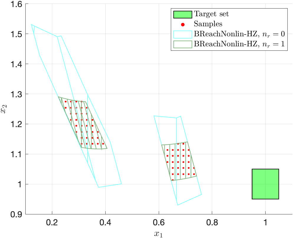
(a) Over-approximation of BRSs based on SOS.

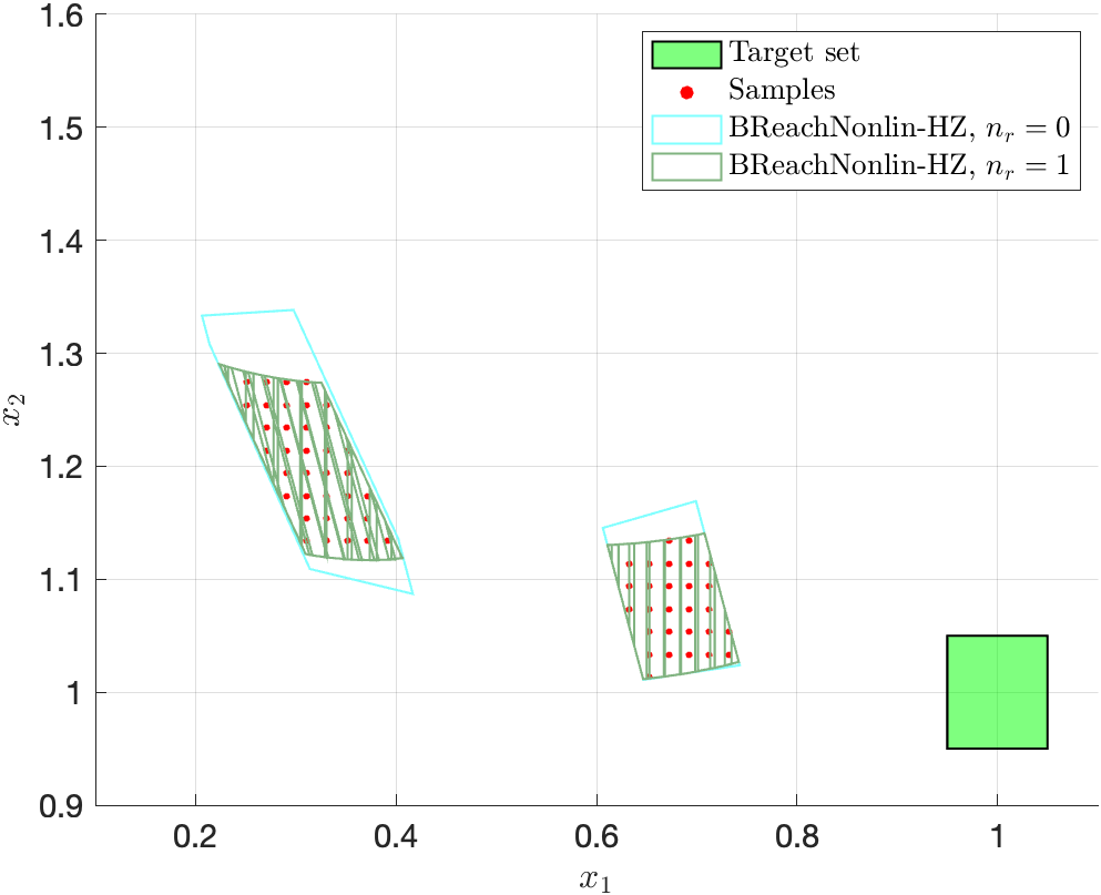
(b) Over-approximation of BRSs based on OVERT.

Figure 2: Over-approximated BRSs without refinement (cyan), the refined over-approximated BRSs (dark green), and samples (red) from the true BRSs for Example 1.

Given the target set $\mathcal{T}=[\![0.95,1.05]\!]\times[\![0.95,1.05]\!]$, Algorithm 1 is employed to over-approximate the BRSs. Note that we use 10 breakpoints to over-approximate the nonlinear term $\bm{x}_{1}^{3}$ via SOS and OVERT and then $\overline{\mathcal{H}}_{f}(\mathcal{X}_{t}^{p},\mathcal{U}_{t}^{p})$ is constructed by following a similar procedure as the example in [20]. Figure 2 shows the simulation results of the over-approximated BRSs (cyan), the one-epoch-refined over-approximated BRSs (dark green), and the samples located inside the true BRSs (red) for two steps. It is observed that all the samples are enclosed by the over-approximated BRSs and the conservativeness is greatly mitigated by the refinement procedure. In addition, with the same number of breakpoints, the computed BRSs by using OVERT are less conservative than those by using SOS.

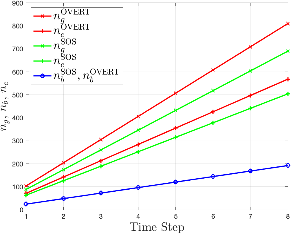
(a) Set complexities.

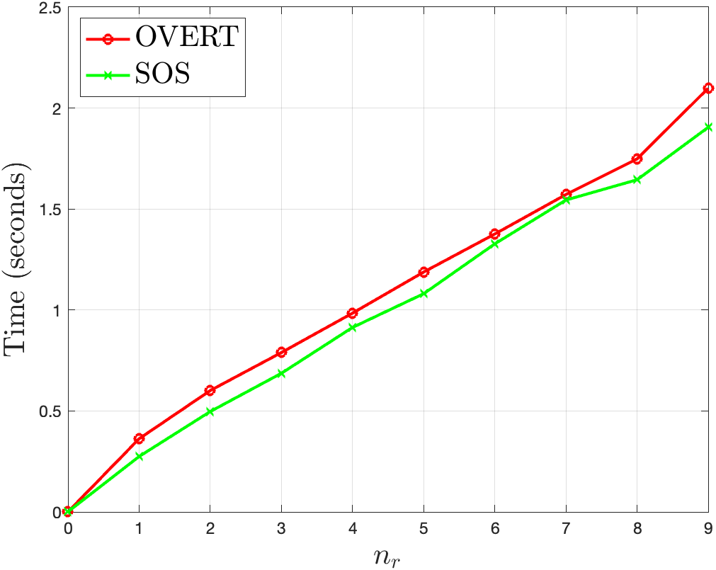
(b) Computation time.

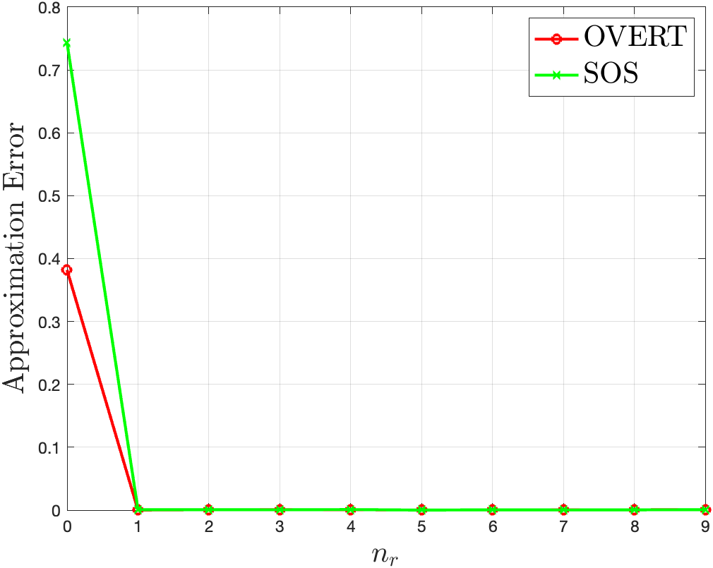
(c) Approximation error.

Figure 3: Comparison of the SOS and OVERT approximation methods at each refinement epoch $n_{r}$ for Example 1.

Figure 3(a) shows the set complexity of the $t$-step BRS via SOS and OVERT for $t=1,2,\cdots,8$. Note that the BRSs and refined BRSs have the same set complexity since the prior sets $\mathcal{X}_{t}^{p}\times\mathcal{U}_{t}^{p}$ are represented by hyper-boxes. The number of generators and equality constraints has a linear growth rate with respect to time steps. In addition, since the number of breakpoints used for over-approximating nonlinear dynamics is the same, the number of binary generators of BRSs is identical in both cases.

To evaluate the trade-off between computation efficiency and approximation accuracy resulting from the refinement procedure, we record the computation time and the approximation error for two-step BRS obtained by Algorithm 1 with different numbers of refinement epochs $n_{r}$. The relative approximation error is computed by the ratio between the volumes of the over-approximated BRS and true BRS as $\text{error}=\frac{V_{\rm over}-V_{\rm true}}{V_{\rm over}}$, where $V_{\rm over}$ and $V_{\rm true}$ are the volume of over-approximation of last-step BRS and true BRS respectively, which are approximated by the Monte Carlo method. Figure 3(b) and Figure 3(c) show the computational time and the approximation error for two-step BRS at each refinement epoch. The computation of BRSs without refinement completes in 0.0006 seconds. The computation time increases almost linearly with respect to the number of refinement epochs due to the fact that the refinement procedure does not affect the set complexity of the computed BRSs. In addition, the approximation error is converged after just one epoch in this example.

Example 2

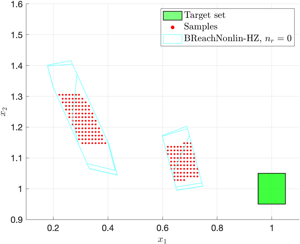
Figure 4: Over-approximated BRSs without refinement (cyan) and samples (red) from the true BRSs for Example 2.

Consider the same Duffing Oscillator model in Example 1. Instead of the ReLU-activated FNN controller, we train a tanh-activated FNN with 5-5 hidden neurons to learn the same control policy given in [28]. We use OVERT with $N=7$ breakpoints to construct the over-approximation of the graph set of FNN $\overline{\mathcal{H}}_{\pi}$ via Theorem 2, and then compute the over-approximated BRSs without refinement with the same configurations as those in Example 1. The simulation results are shown in Figure 4. It is observed that all the samples are enclosed by the over-approximated BRSs.

VI Conclusion

In this paper, we proposed a novel HZ-based approach to over-approximate BRSs of NFSs with nonlinear dynamic models. For NFSs with ReLU activation functions, by combining techniques that over-approximate nonlinear functions with the exact graph set of ReLU-activated FNNs, we showed the closed-form of over-approximated BRSs and a refinement procedure to reduce the conservativeness. In addition, we extended the results to NFSs with piecewise and non-piecewise linear activation functions. The performance of the proposed approach was evaluated using two numerical examples.

References

- [1] S. Dutta, X. Chen, and S. Sankaranarayanan, “Reachability analysis for neural feedback systems using regressive polynomial rule inference,” in Proceedings of the 22nd ACM International Conference on Hybrid Systems: Computation and Control, 2019, pp. 157–168.
- [2] C. Huang, J. Fan, W. Li, X. Chen, and Q. Zhu, “ReachNN: Reachability analysis of neural-network controlled systems,” ACM Transactions on Embedded Computing Systems, vol. 18, no. 5s, pp. 1–22, 2019.
- [3] M. Everett, G. Habibi, C. Sun, and J. P. How, “Reachability analysis of neural feedback loops,” IEEE Access, vol. 9, pp. 163 938–163 953, 2021.
- [4] H.-D. Tran, X. Yang, D. Manzanas Lopez, P. Musau, L. V. Nguyen, W. Xiang, S. Bak, and T. T. Johnson, “NNV: The neural network verification tool for deep neural networks and learning-enabled cyber-physical systems,” in 32nd International Conference on Computer-Aided Verification. Springer, 2020, pp. 3–17.
- [5] M. Fazlyab, M. Morari, and G. J. Pappas, “Safety verification and robustness analysis of neural networks via quadratic constraints and semidefinite programming,” IEEE Transactions on Automatic Control, vol. 67, no. 1, pp. 1–15, 2022.
- [6] Y. Zhang and X. Xu, “Safety verification of neural feedback systems based on constrained zonotopes,” in IEEE 61st Conference on Decision and Control, 2022, pp. 2737–2744.
- [7] ——, “Reachability analysis and safety verification of neural feedback systems via hybrid zonotopes,” in American Control Conference. IEEE, 2023, pp. 1915–1921.
- [8] N. Kochdumper, C. Schilling, M. Althoff, and S. Bak, “Open-and closed-loop neural network verification using polynomial zonotopes,” in NASA Formal Methods Symposium. Springer, 2023, pp. 16–36.
- [9] J. A. Vincent and M. Schwager, “Reachable polyhedral marching (RPM): A safety verification algorithm for robotic systems with deep neural network components,” in IEEE International Conference on Robotics and Automation, 2021, pp. 9029–9035.
- [10] N. Rober, S. M. Katz, C. Sidrane, E. Yel, M. Everett, M. J. Kochenderfer, and J. P. How, “Backward reachability analysis of neural feedback loops: Techniques for linear and nonlinear systems,” IEEE Open Journal of Control Systems, 2023.
- [11] Y. Zhang, H. Zhang, and X. Xu, “Backward reachability analysis of neural feedback systems using hybrid zonotopes,” IEEE Control Systems Letters, vol. 7, pp. 2779–2784, 2023.
- [12] I. Mitchell, A. Bayen, and C. Tomlin, “A time-dependent Hamilton-Jacobi formulation of reachable sets for continuous dynamic games,” IEEE Transactions on Automatic Control, vol. 50, no. 7, pp. 947–957, 2005.
- [13] L. Yang, H. Zhang, J.-B. Jeannin, and N. Ozay, “Efficient backward reachability using the Minkowski difference of constrained zonotopes,” IEEE Transactions on Computer-Aided Design of Integrated Circuits and Systems, vol. 41, no. 11, pp. 3969–3980, 2022.
- [14] N. Rober, M. Everett, and J. P. How, “Backward reachability analysis for neural feedback loops,” in IEEE 61st Conference on Decision and Control, 2022, pp. 2897–2904.
- [15] C. Sidrane, A. Maleki, A. Irfan, and M. J. Kochenderfer, “OVERT: An algorithm for safety verification of neural network control policies for nonlinear systems,” Journal of Machine Learning Research, vol. 23, no. 117, pp. 1–45, 2022.
- [16] T. J. Bird, H. C. Pangborn, N. Jain, and J. P. Koeln, “Hybrid zonotopes: A new set representation for reachability analysis of mixed logical dynamical systems,” Automatica, vol. 154, p. 111107, 2023.
- [17] T. J. Bird and N. Jain, “Unions and complements of hybrid zonotopes,” IEEE Control Systems Letters, vol. 6, pp. 1778–1783, 2021.
- [18] T. J. Bird, “Hybrid zonotopes: A mixed-integer set representation for the analysis of hybrid systems,” Purdue University Graduate School, 2022.
- [19] J. Ortiz, A. Vellucci, J. Koeln, and J. Ruths, “Hybrid zonotopes exactly represent ReLU neural networks,” arXiv preprint arXiv:2304.02755, 2023.
- [20] J. A. Siefert, T. J. Bird, J. P. Koeln, N. Jain, and H. C. Pangborn, “Successor sets of discrete-time nonlinear systems using hybrid zonotopes,” in American Control Conference. IEEE, 2023, pp. 1383–1389.
- [21] ——, “Reachability analysis of nonlinear systems using hybrid zonotopes and functional decomposition,” arXiv preprint arXiv:2304.06827, 2023.
- [22] G. P. McCormick, “Computability of global solutions to factorable nonconvex programs: Part I—Convex underestimating problems,” Mathematical programming, vol. 10, no. 1, pp. 147–175, 1976.
- [23] S. Caratzoulas and C. Floudas, “Trigonometric convex underestimator for the base functions in fourier space,” Journal of optimization theory and applications, vol. 124, no. 2, pp. 339–362, 2005.
- [24] E. Wanufelle, “A global optimization method for mixed integer nonlinear nonconvex problems related to power systems analysis,” Ph. D. dissertation, 2007.
- [25] E. Beale and J. Tomlin, “Special facilities in a general mathematical programming system for nonconvex problems using ordered sets of variables,” Operational Research, vol. 69, pp. 447–454, 01 1969.
- [26] K. He, X. Zhang, S. Ren, and J. Sun, “Delving deep into rectifiers: Surpassing human-level performance on imagenet classification,” in Proceedings of the IEEE International Conference on Computer Vision, 2015, pp. 1026–1034.
- [27] S. R. Dubey, S. K. Singh, and B. B. Chaudhuri, “Activation functions in deep learning: A comprehensive survey and benchmark,” Neurocomputing, vol. 503, pp. 92–108, 2022.
- [28] T. Dang and R. Testylier, “Reachability analysis for polynomial dynamical systems using the Bernstein expansion.” Reliabable Computing, vol. 17, no. 2, pp. 128–152, 2012.