Distillation Improves Visual Place Recognition for Low-Quality Queries

Abstract

The shift to online computing for real-time visual localization often requires streaming query images/videos to a server for visual place recognition (VPR), where fast video transmission may result in reduced resolution or increased quantization. This compromises the quality of global image descriptors, leading to decreased VPR performance. To improve the low recall rate for low-quality query images, we present a simple yet effective method that uses high-quality queries only during training to distill better feature representations for deep-learning-based VPR, such as NetVLAD. Specifically, we use mean squared error (MSE) loss between the global descriptors of queries with different qualities, and inter-channel correlation knowledge distillation (ICKD) loss over their corresponding intermediate features. We validate our approach using the both Pittsburgh 250k dataset and our own indoor dataset with varying quantization levels. By fine-tuning NetVLAD parameters with our distillation-augmented losses, we achieve notable VPR recall-rate improvements over low-quality queries, as demonstrated in our extensive experimental results. We believe this work not only pushes forward the VPR research but also provides valuable insights for applications needing dependable place recognition under resource-limited conditions.

I Introduction

Visual Place Recognition (VPR) has rapidly become a foundational component in the realm of machine recognition. By harnessing visual cues, devices can recognize and recall previously visited locations [1]. This capability extends beyond novelty, proving invaluable in applications ranging from robots navigating intricate industrial settings to augmented reality systems overlaying digital data onto the physical world [2, 3, 4].

The adaptability of VPR across diverse environments has expanded its use cases. From smartphones to autonomous vehicles, the need for efficient and precise VPR systems is escalating. However, this rising demand, especially in consumer devices, introduces complex challenges. A primary concern is the burgeoning growth in scene diversity and volume, leading to expansive databases that pose storage challenges for devices with limited capacity [5].

Furthermore, the pursuit of accuracy has spurred the creation of intricate models [6, 7, 8]. While these models excel at deriving detailed global descriptors, they come at a cost: their computational demands hinder real-time, offline VPR processing on standard devices due to significant computational overheads [9].

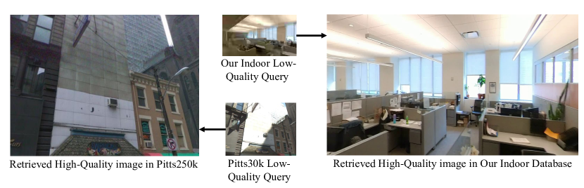
Figure 1: Visual Place Recognition with Low-Quality Query Images: Leveraging our proposed distillation neural network and specific loss configurations, we fine-tuned our model on the Pitts250k database using NetVLAD as the backbone, enabling better database image retrieval from significantly compressed images. Centrally depicted in this figure are compressed images from the Pitts30k test dataset (downsampled to $240\times 180$) and our collected video from an indoor scene (downsampled to $360\times 203$ and quantized with a parameter of $48$). Flanking these are the retrieved high-quality database images with resolutions of $640\times 480$ (left) and $1440\times 810$ (right).

Transitioning to online computation might seem a solution, but it presents its own challenges. Transmitting query images from devices to servers in real-time becomes a bottleneck in our fast-paced world. Balancing video stream bitrate with network bandwidth often leads to solutions like reducing video resolution or increasing quantization. However, these measures, while aiding transmission, degrade the global descriptor quality, impacting the VPR recall rate [10].

Addressing these challenges, our research offers several key contributions:

• We developed a novel approach to train models on low-quality images, aiming to emulate the behavior of their high-quality counterparts.

• Exploration and evaluation of three distinct loss functions, with a special emphasis on the combination of inter-channel correlation knowledge distillation (ICKD) loss [11] and MSE loss, tailored to enhance the performance of the NetVLAD model [6] with low-quality query images.

• Through our approach, the student branch of our model was meticulously fine-tuned to mirror its teacher counterpart, leading to significant improvements in recall rates for low-quality query images, as validated on a unique indoor dataset with varied quantization levels.

Figure 1 demonstrates the retrieval of high-quality images using low-quality queries, highlighting the efficacy of our fine-tuned NetVLAD parameters using the improved loss function.

II Related Work

Visual Place Recognition (VPR) has witnessed substantial advancements in methodologies and techniques over the years [6, 7, 12, 13, 14, 15]. The primary objective of VPR has always been to recognize places using visual cues. This section delves into the key developments in VPR, setting the stage for our novel contributions by contrasting them with existing methodologies.

Global Descriptors in VPR: The essence of VPR lies in the image descriptor. Global image descriptors have gained prominence due to their comprehensive scene representation capabilities. Initial VPR techniques, such as GIST [16], SIFT [17], and VLAD [18], revolved around compact image representations based on hand-crafted local features. The advent of deep learning, epitomized by NetVLAD [6], merged traditional descriptor generation with neural networks. However, the enhanced complexity of these descriptors, while improving accuracy, posed computational challenges, particularly in resource-constrained offline settings [9].

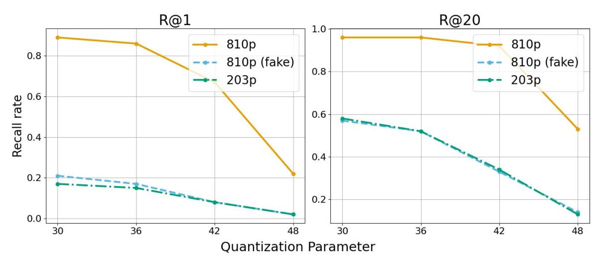
Figure 2: Super-resolution’s limited impact on VPR recall rate. Using Real-ESRGAN, we generated $4\times$ super-resolution images, upscaled from $360\times 203$ to $1440\times 810$. Comparing the VPR performance of these super-resolution images, original low-resolution images ($360\times 203$), and original high-quality images ($1440\times 810$) from our indoor dataset with NetVLAD, we found that super-resolution did not enhance VPR retrieval.

Adaptation to Image Quality: The quality of images is pivotal for VPR performance. Recent studies, such as those by Tomita et al. [10], highlight the detrimental impact of reduced resolution on VPR recall rates. Super-resolution techniques [19], proposed to ameliorate degraded images, often entail computational compromises. As illustrated in Figure 2 using Real-ESRGAN [20], these methods did not significantly enhance VPR recall rates, leading us to explore knowledge distillation from high-quality imagery.

Knowledge Distillation and Transfer Learning in VPR: Knowledge distillation and transfer learning have emerged as prominent strategies in various machine learning domains [21, 22, 23, 11]. These techniques aim to transfer insights from intricate models to simpler, efficient counterparts. In the VPR domain, this translates to a harmonious blend of accuracy and efficiency. Our approach deviates from conventional methods, focusing on training with low-quality images to emulate their high-quality counterparts. We incorporate bespoke loss functions tailored to VPR’s distinct challenges. Contrary to prevalent distillation techniques [21, 22, 23], our model processes varying resolution images in its student and teacher branches, prompting us to employ the Inter-channel correlation knowledge distillation strategy [11].

Evaluation Datasets in VPR Datasets are pivotal for validating VPR methodologies. While traditional datasets like Pittsburgh 250k [24], MSLS [25], GSV-Cities [26], NYU-VPR [27], and others have been invaluable, the evolving VPR landscape necessitates datasets that account for image degradation, especially post-compression. Our contribution includes a unique indoor dataset with varied quantization levels, aiming to provide a more holistic understanding of VPR challenges and potential solutions.

III Proposed Approach

Visual Place Recognition (VPR) has seen a plethora of methodologies, each striving to enhance place recognition’s precision and efficiency. Our approach pivots towards knowledge distillation, a technique that has demonstrated its efficacy across various machine learning domains. By employing this technique, we aim to enable a student network to mimic the intricate behavior of a more sophisticated teacher network, even when processing images of varying quality. Our methodology is rooted in the NetVLAD algorithm [6], which forms the backbone of our distillation framework. The following subsections provide a detailed breakdown of our approach, elucidating the mechanics and rationale behind each component.

III-A Distillation model

Central to our approach is the distillation model, denoted as $f$, illustrated in Figure 3. Designed as a dual-branch system, it consists of the student branch $f_{s}$ and the teacher branch $f_{t}$. This design facilitates parallel processing of images with different resolutions. Both branches utilize the VGG-16 architecture [28] as their feature encoder, represented by $f^{\theta}_{s}$ and $f^{\theta}_{t}$ for the student and teacher branches, respectively. These encoders are integrated with the NetVLAD pooling layers, $g^{\phi}_{s}$ and $g^{\phi}_{t}$.

The student branch processes a low-quality image $I^{l}$ of dimensions $w\times h$, while the teacher branch handles a high-quality image $I^{h}$ with dimensions $W\times H$. The resulting latent codes are denoted as $z^{l}$ and $z^{h}$ for the student and teacher, respectively. These codes are further refined into $v^{l}$ and $v^{h}$ through pooling.

Subsequent sections delve into the three loss functions we evaluated. We further discuss the optimal loss combinations that we ultimately adopted, elucidating our efforts to train $f_{s}$ to closely emulate the behavior of $f_{t}$.

Figure 3: Illustration of the proposed knowledge distillation approach. The diagram presents a parallel dual-branch system: the student branch processes a low-quality image $I^{l}$, while the teacher branch, with fixed parameters, deals with its high-quality counterpart $I^{h}$. Through loss $L_{\theta 1}$, we ensure that the Inter-Channel Correlation (ICC) matrix $\hat{C^{l}}$ from the student branch closely matches the teacher-derived $\hat{C^{h}}$. Similarly, we use the MSE loss $L_{\theta 2}$ to make the student’s final vector $v^{l}$ resemble the teacher’s $v^{h}$. Lastly, the triplet loss $L_{\theta 3}$ ensures that the vector $v^{l}$ from the query image $I^{l}$ aligns more closely with the vector (${v^{l}_{p}}_{i}$) from a proximate image and diverges from the vector (${v^{l}_{n}}_{j}$) of a distant image.

III-B Proposed losses

Inter-channel Correlation Knowledge Distillation (ICKD) Loss [11]: This loss operates on the latent codes $z^{l}$ and $z^{h}$. Given the size differences between inputs $I^{l}$ and $I^{h}$, the latent codes $z^{l}$ and $z^{h}$ differ in dimensions. Traditional distillation losses, which typically require matching dimensions for the latent codes, are not directly applicable. The ICKD loss overcomes this by computing an Inter-Channel Correlation (ICC) and urging the student’s ICC to approximate the teacher’s ICC.

Assuming $z^{l}$ has dimensions $c\times w^{\prime}\times h^{\prime}$, it is flattened to produce the vector $p^{l}$ with dimensions $c\times w^{\prime}h^{\prime}$. This vector undergoes normalization along its third dimension, resulting in $\hat{p^{l}}=\frac{p^{l}}{\|p^{l}\|}$. The subsequent ICC matrix $C^{l}=\hat{p^{l}}\times\hat{p^{l}}^{T}$ with dimensions $c\times c$ is normalized to $\hat{C^{l}}=\frac{C^{l}}{\|C^{l}\|}$. A similar procedure for $z^{h}$ yields $\hat{C^{h}}$.

The ICKD loss, formulated to ensure the student branch mirrors the teacher branch, is defined as:

$$L_{\theta 1}=\|\hat{C^{l}}-\hat{C^{h}}\|_{2}.$$ (1)

Mean Squared Error (MSE) Loss: This loss evaluates the discrepancy between the output vectors $v^{l}$ and $v^{h}$. By employing the MSE loss, we aspire for the student branch’s output vector $v^{l}$ to closely mirror $v^{h}$ from the teacher branch. The MSE loss is expressed as:

$$L_{\theta 2}=\|v^{l}-v^{h}\|_{2}^{2}.$$ (2)

Our rationale for using $L_{\theta 2}$ is its potential to enable the student branch $f_{s}$ to glean insights from the teacher branch $f_{t}$. By minimizing the squared discrepancies between the vectors, we aim for the student branch to emulate the teacher’s outputs and internalize the intricate patterns and knowledge inherent in the teacher branch.

Weakly Supervised Triplet Ranking Loss: Applied exclusively to the student branch $f_{s}$, this loss draws inspiration from the mechanism employed by NetVLAD. It ensures that the descriptor extracted from a query image, represented as $v^{l}$, aligns more closely with the descriptor of a proximate image, $\{v^{l}_{p}\}$, than with the descriptor of a distant image, $\{v^{l}_{n}\}$. The goal is to satisfy the inequality $d_{\theta}(v^{l},v^{l}_{p})<d_{\theta}(v^{l},v^{l}_{n})$, where $d_{\theta}$ denotes the Euclidean distance between descriptors.

The triplet loss is articulated as:

$$L_{\theta 3}=\sum_{j}l\left(\min_{i}d_{\theta}^{2}(v^{l},{v^{l}_{p}}_{i})-d_{\theta}^{2}(v^{l},{v^{l}_{n}}_{j})+m\right).$$ (3)

In this equation, $l$ represents the hinge loss, defined as $l(x)=\max(x,0)$. The term $m$ is a margin parameter, ensuring a buffer between positive and negative pairs, thereby enhancing the discriminative capabilities of the learned embeddings. The component $\min_{i}d_{\theta}^{2}(v^{l},{v^{l}_{p}}_{i})$ selects the descriptor of the most congruent image as estimated by the student model $f_{s}$, ensuring the loss is attuned to the nearest matches.

Composite Loss: Our objective is to assess the effectiveness of a combined loss function relative to the individual application of the aforementioned losses. We compute a cumulative loss as:

$$L=L_{\theta_{1}}+\alpha L_{\theta_{2}}+\beta L_{\theta_{3}}.$$ (4)

In this equation, $\alpha$ and $\beta$ are weighting coefficients for the respective loss components, facilitating fine-tuning and balancing the influence of each loss within the composite function. However, our experiments revealed that the triplet loss $L_{\theta_{3}}$ actually hindered network performance, so our final loss becomes:

$$L=L_{\theta_{1}}+\alpha L_{\theta_{2}}.$$ (5)

IV Experimental Setup

To validate the efficacy of our proposed distillation model, we meticulously designed an experimental setup. This setup encompasses two datasets: the renowned VPR dataset, Pitts250k [24], and a novel dataset curated by us, emphasizing the effects of downsampling and quantizing input videos. In the subsequent sections, we detail the datasets’ characteristics and delineate our experimental configurations.

IV-A Dataset

Pitts250k Dataset: The Pitts250k dataset stands as a cornerstone in VPR research, boasting over $250,000$ diverse urban images sourced from Pittsburgh. Its rich temporal variability, high-quality imagery, and precise geotagged information render it invaluable for our study. To systematically investigate the implications of image resolution on VPR, we partitioned the dataset into three segments: $175k$ images for training, $52.5k$ as a database, and $22.5k$ for validation. In addition, we designated Pitts30k-val as our query set. The images, originally at a resolution of $640\times 480$, underwent downsampling to three distinct resolutions, namely:

• Resolutions $r_{\theta}$: $240p$ ($320\times 240$), $180p$ ($240\times 180$)

Our Dataset: To bridge the gap in indoor VPR data and delve deeper into the nuances of video bitrate influences, we curated a dataset from the 6th floor of the Lighthouse Guild. Recognizing the spatial constraints inherent in existing indoor VPR datasets [29, 27], our dataset accentuates the potential of video quantization for real-time localization.

Our dataset comprises $8$ videos, captured using the Insta360 camera, providing a panoramic $360$-degree view. Each frame, with dimensions $5760\times 2880$, was evenly segmented into $18$ perspective images horizontally, each offering a $90$-degree field of view and dimensions $1440\times 810$. These images were subsequently assembled into perspective videos, which were subjected to both downsampling and quantization, resulting in:

• Resolutions $r_{\theta}$: $405p$ ($720\times 405$), $203p$ ($360\times 203$)

• Quantization Parameters $q_{\theta}$: $30$, $33$, $36$, $39$, $42$, $45$, $48$

After processing, frames were meticulously extracted from the videos. Leveraging the prowess of the ORB feature extractor [30], images with local features fewer than $100$ were excluded, ensuring the dataset’s integrity and quality.

To ascertain the ground truth location for each image, we employed a combination of OpenVSLAM [31] and the Aligner GUI from the UNav system [32]. Initially, OpenVSLAM was instrumental in constructing a sparse map, where every $2D$ feature on an image frame corresponded to a $3D$ location in the map, and the image frame’s $6$ DoF pose was determined. Subsequently, the Aligner GUI facilitated the identification of correspondences between the $3D$ locations and their respective $2D$ positions on the floor plan, culminating in a transformation matrix. This matrix was pivotal in mapping all $3D$ locations and $6$ DoF poses onto the floor plan. A salient feature of this methodology is its adeptness in aligning sparse maps from disparate videos, irrespective of when or where they were recorded within a scene, onto a unified coordinate frame using the floor as a reference. Given the uniformity of the recording floor, the elevation (or the $z$-axis coordinate) was deemed inconsequential. As a result, each image was assigned precise floor plan coordinates. After applying the floor plan’s measurement scale, the actual $2D$ locations were derived, serving as the ground truth for our dataset.

IV-B Distillation Setup

Loss	$1$	$2$	$3$	$4$	$5$	$6$	$7$
$L_{\theta_{1}}$ (MSE)
$L_{\theta_{2}}$ (ICKD)
$L_{\theta_{3}}$ (Triplet)

Table I: Various loss combinations across seven training configurations to assess the influence of individual loss components.

Training Configuration: Our training regimen is meticulously designed to optimize the performance of our distillation model. The high-quality image $I^{h}$ is channeled into the teacher branch $f_{t}$, while the low-quality image $I^{l}$ is directed to the student branch $f_{s}$. To strike a balance between the influences of each loss function, we empirically set the coefficients to $\alpha=10^{5}$ and $\beta=10^{4}$. The teacher branch $f_{t}$ processes raw images without any modifications. For the student branch $f_{s}$ operating on the Pitts250k dataset, we set $r_{\theta}=180p$. For our proprietary dataset, we establish $r_{\theta}=203p$ and $q_{\theta}=30$. The learning rate is initialized at $10^{-5}$ and is modulated by a decay factor of $2\times 10^{-11}$, further adjusted by an exponential rate of $0.99999$.

To discern the impact of each loss component on the network’s performance and to identify the optimal loss configuration, we experimented with seven distinct combinations of the loss functions as defined in Equation (4). These combinations are detailed in Table I.

Each training experiment spanned $10$ epochs. For the triplet loss, during each iteration, we utilized $5$ negative descriptors, represented as $v^{l}_{n}$.

Evaluation Metrics: For our assessment, we employed the optimal model to evaluate images across a spectrum of low resolutions and quantization levels.

Our evaluation methodology aligns with the established conventions in place recognition, as delineated in references [6, 7, 33, 8, 34]. A query image is deemed accurately localized if one of the top $N$ retrieved database images is within $d$ meters of the query’s true position. Notably, when validating on our indoor dataset, a retrieved image must also pass a geometric verification with a threshold of $20$ inliers to be classified as accurately localized. The ratio of successfully retrieved query images serves as our model’s performance metric. For the Pitts250k dataset, we employ $N$ values of 1, 5, and 10, with $d$ fixed at 25 meters, in line with NetVLAD [6]. For our dataset, we select $N$ from the set {1, 10}, and $d$ varies between $1$ to $10$ meters.

V Results and Discussions

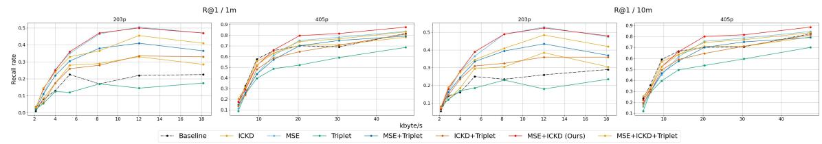
Figure 4: Validation on Our Dataset: Using $7$ distinct loss combinations detailed in Table I, our model was trained on the Pitts250k outdoor dataset at a resolution of $180p$. We then validated on our indoor dataset with resolutions of $405p$ and $203p$, using quantization parameters spanning from $30$ to $48$ in intervals of $3$. It’s important to note that the database images retrieved are of the original high resolution ($810p$). The video’s $kbyte/s$ metric, representing each combination of resolution and quantization, is plotted against the $x$-axis, with the recall rate on the $y$-axis. The left pair of subfigures represent tests under the recall rate R@1 with a $1m$ threshold, while the right pair use a $10m$ threshold. The first and third subfigures are results from the $203p$ tests, and the second and fourth from the $405p$ tests. Notably, the MSE loss (combination $1$) and the combined MSE+ICKD loss (combination $4$) show superior performance on the $203p$ tests. However, the latter exhibits greater adaptability, outperforming on the $405p$ tests, indicating the beneficial role of the ICKD loss in training. Furthermore, the underperformance of combination $3$ and the comparison between $4$ and $7$ suggest that the triplet loss may be detrimental when training with low-quality images.

Model	180p	240p
	R@1/5/10	R@1/5/10
Baseline	0.1520/0.2680/0.3260	0.2590/0.3900/0.4350
ICKD	0.1800/0.2930/0.3450	0.2280/0.3300/0.3830
MSE	0.2720/0.3860/0.4320	0.2880/0.3940/0.4430
Triplet	0.0730/0.1690/0.2300	0.1400/0.2660/0.3150
MSE+Triplet	0.2540/0.3660/0.4140	0.2780/0.3920/0.4350
ICKD+Triplet	0.1730/0.3000/0.3620	0.2320/0.3490/0.3900
MSE+ICKD (Ours)	0.2580/0.3700/0.4120	0.2970/0.3950/0.4450
MSE+ICKD+Triplet	0.2500/0.3540/0.4060	0.2900/0.3950/0.4400

Table II: VPR recall rates on the Pitts30k Dataset: Using models pretrained on the Pitts250k $180p$ dataset, we evaluated performance of recall R@1,R@5 and R@10 on the Pitts30k dataset at resolutions of $180p$ and $240p$ under various loss configurations (Table I). The results indicate that the model trained with setting $1$ (MSE loss), excels for $180p$ queries. However, its adaptability is surpassed by the model trained with setting $4$, which combines the MSE and ICKD losses, as evidenced by its superior performance on $240p$ queries.

Our experiments have provided valuable insights, emphasizing the effectiveness of our proposed distillation model. In this section, we delve into a comprehensive analysis of our results, contrasting the performance across various loss settings and underscoring the merits of our distillation approach.

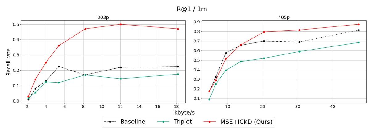
Figure 5: Training and Validation on Our Dataset: To demonstrate the adaptability of our proposed model, we trained and validated it on our indoor dataset using two loss settings: $3$ (Triplet) and $4$ (MSE+ICKD). These results were then juxtaposed with the baseline pretrained model from NetVLAD. The figure underscores the efficacy of our distillation approach, consistently achieving high VPR recall rates across a wide range of byte rates for two distinct resolutions.

Initially, we fine-tuned the NetVLAD network [6] using $7$ distinct loss settings, as detailed in Table I. This fine-tuning was performed on the Pitts250k dataset at a resolution of $180p$. Following this, we evaluated the trained models on low-quality queries, specifically $180p$ and $240p$ from the Pitts30k dataset, while using a high-quality database of $640p$ from Pitts250k. Additionally, we conducted tests on resolutions of $203p$ and $405p$ from our dataset, utilizing all available quantization parameters, to query against the original high-quality images set at $810p$. The detailed outcomes of these tests are presented in the subsequent sections.

V-A Quantitative results

Validation on Pitts30k. We assessed the performance of the pretrained model and its fine-tuned counterparts, each trained using one of the $7$ loss settings (Table I), on the Pitts30k dataset. The pretrained model serves as our benchmark. As depicted in Table II, the model trained with loss setting $1$ (MSE loss) surpasses other configurations, including the baseline, for $180p$ queries. This highlights the potency of our distillation framework. Introducing the ICKD loss (loss setting $4$) enhances the model’s adaptability to the higher $240p$ resolution. We infer that the ICKD loss encourages the low-quality branch to emulate the inter-channel similarities of the feature encoders from the teacher branch. Consequently, when validated on a higher resolution, the model continues to mimic these channel similarities, refining the descriptor’s quality. Notably, our results indicate that the triplet loss on the low-quality branch hampers the global descriptor’s quality.

Generalization study. While the efficacy of the fine-tuned model was validated on the Pitts30k dataset, both Pitts250k and Pitts30k originate from similar outdoor scenes. We aimed to ascertain the model’s generalizability to our distinct indoor dataset.

To this end, we tested our dataset using the best model from each of the $7$ loss settings, all trained on the Pitts250k dataset. Evaluating across different quantization parameters for each resolution in our dataset, we computed the $kbyte/s$ for each parameter. This was used as the $x$-axis, with the recall rate at R@1 and thresholds of 1m and 10m as the $y$-axis, culminating in Figure 4. The results affirm that our model, fine-tuned on Pitts250k using loss setting $4$ (MSE+ICKD losses), is superior in terms of generalization, validating our distillation model’s robustness.

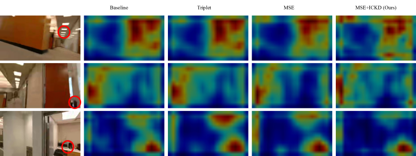
Figure 6: Model’s Area of Focus. This figure presents heatmaps indicating the regions of interest for four models trained using different loss settings, as detailed in Table I. The red circles on the left query images highlight the key areas of interest. In the top image, the model trained with the MSE+ICKD loss concentrates more on specific objects, in contrast to other models which generalize over a broader area. In the middle image, the MSE+ICKD-trained model notably focuses on the table corner in another room visible through the door. While the model trained solely on the MSE loss also acknowledges this area, its attention is less pronounced. Other loss settings overlook this detail. In the bottom image, the MSE+ICKD model predominantly centers its attention on the table laden with distinct objects, aiding location identification. However, other models are also drawn to the light, a potential source of visual aliasing.

Training on Our Dataset: We were keen to investigate the model’s performance when trained on our indoor-scene dataset at $203p$. Utilizing loss settings $3$ (Triplet) and $4$ (MSE+ICKD), we fine-tuned the models. These were then validated against the NetVLAD pretrained model, serving as our baseline, on resolutions $203p$ and $405p$. The recall rates at R@1 with a threshold of $1m$ are depicted in Figure 5. Notably, the model fine-tuned with loss setting $4$ consistently surpasses its counterparts across nearly all byte rates for both resolutions, underscoring the potency of our proposed approach.

Training Across All Resolutions: Given the impressive performance of our model when trained on low-quality images, we were motivated to investigate whether training on the entire spectrum of image resolutions could further boost its efficacy. However, as depicted in Table III, even though models trained with the Triplet and CS+MSE loss settings surpass the baseline, their improvements are relatively subdued in comparison to those trained exclusively on low-quality images.

V-B Qualitative results

To discern why the distillation model trained on Pitts250k with loss setting $4$ (MSE+ICKD) surpasses the performance of other loss configurations, we visualized the attention heatmaps of the feature encoder, as depicted in Figure 6. We juxtaposed the attention heatmap from loss setting $4$ against those derived from models trained with two other loss settings: $1$ (MSE) and $3$ (Triplet). Observably, under loss setting $4$, the model predominantly concentrates on critical regions while overlooking areas prone to visual aliasing. This focused attention might underpin the superior performance exhibited by this particular loss setting.

	@1		@20
	1m	10m	1m	10m
Baseline	0.4785	0.5028	0.7607	0.8763
Triplet	0.4978	0.5246	0.7657	0.8763
MSE+ICKD (Ours)	0.5098	0.5317	0.7857	0.8893

Table III: VPR Recall Rates Across Models Trained on Comprehensive Image Sets: Performance evaluation of models trained and tested with various loss settings on our indoor dataset, encompassing all resolutions and quantization parameters.

VI Conclusion

In this work, we have empirically demonstrated the efficacy of knowledge distillation for enhancing the performance of Visual Place Recognition (VPR) in scenarios characterized by compromised image quality. The observed improvements in recall rates on both the Pitts250k and our custom indoor dataset underscore the robustness and generalizability of the proposed model. Through a systematic analysis of various loss functions, we identified that a combination of the Mean Squared Error (MSE) loss and the Inter-channel Correlation Knowledge Distillation (ICKD) loss yielded optimal results.

Limitation: However, it is pertinent to note that while our fine-tuned model exhibits commendable performance on low-quality queries, the VPR performance gap between low-quality queries and high-quality ones is still non-negligible. This means when seeking better localization performance, using higher-quality queries is still an easy option even with the communication bandwidth constraints. The performance gap needs to be further reduced to make VPR from low-quality queries more appealing and acceptable than naively depending on high-quality queries.

Future Work: As a future direction, we intend to further refine the loss functions, explore alternative combinations, and potentially investigate different model architectures to address this observed limitation. Additionally, there is a clear avenue to expand our indoor dataset to include a wider variety of environments and associated challenges.

References

- Garg et al. [2021] S. Garg, T. Fischer, and M. Milford, “Where is your place, visual place recognition?” arXiv preprint arXiv:2103.06443, 2021.
- Doan et al. [2019] A.-D. Doan, Y. Latif, T.-J. Chin, Y. Liu, T.-T. Do, and I. Reid, “Scalable place recognition under appearance change for autonomous driving,” in Proceedings of the IEEE/CVF International Conference on Computer Vision, 2019, pp. 9319–9328.
- Yin et al. [2019] P. Yin, L. Xu, X. Li, C. Yin, Y. Li, R. A. Srivatsan, L. Li, J. Ji, and Y. He, “A multi-domain feature learning method for visual place recognition,” in 2019 International conference on robotics and automation (ICRA). IEEE, 2019, pp. 319–324.
- Xin et al. [2019] Z. Xin, Y. Cai, T. Lu, X. Xing, S. Cai, J. Zhang, Y. Yang, and Y. Wang, “Localizing discriminative visual landmarks for place recognition,” in 2019 International conference on robotics and automation (ICRA). IEEE, 2019, pp. 5979–5985.
- Kornilova et al. [2023] A. Kornilova, I. Moskalenko, T. Pushkin, F. Tojiboev, R. Tariverdizadeh, and G. Ferrer, “Dominating set database selection for visual place recognition,” arXiv preprint arXiv:2303.05123, 2023.
- Arandjelovic et al. [2016] R. Arandjelovic, P. Gronat, A. Torii, T. Pajdla, and J. Sivic, “Netvlad: Cnn architecture for weakly supervised place recognition,” in Proceedings of the IEEE conference on computer vision and pattern recognition, 2016, pp. 5297–5307.
- Ali-Bey et al. [2023] A. Ali-Bey, B. Chaib-Draa, and P. Giguere, “Mixvpr: Feature mixing for visual place recognition,” in Proceedings of the IEEE/CVF Winter Conference on Applications of Computer Vision, 2023, pp. 2998–3007.
- Berton et al. [2022] G. Berton, C. Masone, and B. Caputo, “Rethinking visual geo-localization for large-scale applications,” in Proceedings of the IEEE/CVF Conference on Computer Vision and Pattern Recognition, 2022, pp. 4878–4888.
- Garg and Milford [2020] S. Garg and M. Milford, “Fast, compact and highly scalable visual place recognition through sequence-based matching of overloaded representations,” in 2020 IEEE international conference on robotics and automation (ICRA). IEEE, 2020, pp. 3341–3348.
- Tomita et al. [2023] M.-A. Tomita, B. Ferrarini, M. Milford, K. McDonald-Maier, and S. Ehsan, “Visual place recognition with low-resolution images,” arXiv preprint arXiv:2305.05776, 2023.
- Liu et al. [2021] L. Liu, Q. Huang, S. Lin, H. Xie, B. Wang, X. Chang, and X. Liang, “Exploring inter-channel correlation for diversity-preserved knowledge distillation,” in Proceedings of the IEEE/CVF International Conference on Computer Vision, 2021, pp. 8271–8280.
- Ge et al. [2020] Y. Ge, H. Wang, F. Zhu, R. Zhao, and H. Li, “Self-supervising fine-grained region similarities for large-scale image localization,” in Computer Vision–ECCV 2020: 16th European Conference, Glasgow, UK, August 23–28, 2020, Proceedings, Part IV 16. Springer, 2020, pp. 369–386.
- Jin Kim et al. [2017] H. Jin Kim, E. Dunn, and J.-M. Frahm, “Learned contextual feature reweighting for image geo-localization,” in Proceedings of the IEEE Conference on Computer Vision and Pattern Recognition, 2017, pp. 2136–2145.
- Liu et al. [2019] L. Liu, H. Li, and Y. Dai, “Stochastic attraction-repulsion embedding for large scale image localization,” in Proceedings of the IEEE/CVF International Conference on Computer Vision, 2019, pp. 2570–2579.
- Seymour et al. [2019] Z. Seymour, K. Sikka, H.-P. Chiu, S. Samarasekera, and R. Kumar, “Semantically-aware attentive neural embeddings for long-term 2d visual localization,” in British Machine Vision Conference (BMVC), 2019.
- Oliva and Torralba [2001] A. Oliva and A. Torralba, “Modeling the shape of the scene: A holistic representation of the spatial envelope,” International journal of computer vision, vol. 42, pp. 145–175, 2001.
- Lowe [2004] D. G. Lowe, “Distinctive image features from scale-invariant keypoints,” International journal of computer vision, vol. 60, pp. 91–110, 2004.
- Jégou et al. [2010] H. Jégou, M. Douze, C. Schmid, and P. Pérez, “Aggregating local descriptors into a compact image representation,” in 2010 IEEE computer society conference on computer vision and pattern recognition. IEEE, 2010, pp. 3304–3311.
- Ledig et al. [2017] C. Ledig, L. Theis, F. Huszár, J. Caballero, A. Cunningham, A. Acosta, A. Aitken, A. Tejani, J. Totz, Z. Wang et al., “Photo-realistic single image super-resolution using a generative adversarial network,” in Proceedings of the IEEE conference on computer vision and pattern recognition, 2017, pp. 4681–4690.
- Wang et al. [2021] X. Wang, L. Xie, C. Dong, and Y. Shan, “Real-esrgan: Training real-world blind super-resolution with pure synthetic data,” in Proceedings of the IEEE/CVF international conference on computer vision, 2021, pp. 1905–1914.
- Hinton et al. [2015] G. Hinton, O. Vinyals, and J. Dean, “Distilling the knowledge in a neural network,” arXiv preprint arXiv:1503.02531, 2015.
- Hui et al. [2018] Z. Hui, X. Wang, and X. Gao, “Fast and accurate single image super-resolution via information distillation network,” in Proceedings of the IEEE conference on computer vision and pattern recognition, 2018, pp. 723–731.
- Tung and Mori [2019] F. Tung and G. Mori, “Similarity-preserving knowledge distillation,” in Proceedings of the IEEE/CVF international conference on computer vision, 2019, pp. 1365–1374.
- Torii et al. [2013] A. Torii, J. Sivic, T. Pajdla, and M. Okutomi, “Visual place recognition with repetitive structures,” in Proceedings of the IEEE conference on computer vision and pattern recognition, 2013, pp. 883–890.
- Warburg et al. [2020] F. Warburg, S. Hauberg, M. Lopez-Antequera, P. Gargallo, Y. Kuang, and J. Civera, “Mapillary street-level sequences: A dataset for lifelong place recognition,” in Proceedings of the IEEE/CVF conference on computer vision and pattern recognition, 2020, pp. 2626–2635.
- Ali-bey et al. [2022] A. Ali-bey, B. Chaib-draa, and P. Giguère, “Gsv-cities: Toward appropriate supervised visual place recognition,” Neurocomputing, vol. 513, pp. 194–203, 2022.
- Sheng et al. [2021] D. Sheng, Y. Chai, X. Li, C. Feng, J. Lin, C. Silva, and J.-R. Rizzo, “Nyu-vpr: long-term visual place recognition benchmark with view direction and data anonymization influences,” in 2021 IEEE/RSJ International Conference on Intelligent Robots and Systems (IROS). IEEE, 2021, pp. 9773–9779.
- Simonyan and Zisserman [2014] K. Simonyan and A. Zisserman, “Very deep convolutional networks for large-scale image recognition,” arXiv preprint arXiv:1409.1556, 2014.
- Lee et al. [2021] D. Lee, S. Ryu, S. Yeon, Y. Lee, D. Kim, C. Han, Y. Cabon, P. Weinzaepfel, N. Guérin, G. Csurka et al., “Large-scale localization datasets in crowded indoor spaces,” in Proceedings of the IEEE/CVF Conference on Computer Vision and Pattern Recognition, 2021, pp. 3227–3236.
- Rublee et al. [2011] E. Rublee, V. Rabaud, K. Konolige, and G. Bradski, “Orb: An efficient alternative to sift or surf,” in 2011 International conference on computer vision. Ieee, 2011, pp. 2564–2571.
- Sumikura et al. [2019] S. Sumikura, M. Shibuya, and K. Sakurada, “OpenVSLAM: A Versatile Visual SLAM Framework,” in Proceedings of the 27th ACM International Conference on Multimedia, ser. MM ’19. New York, NY, USA: ACM, 2019, pp. 2292–2295. [Online]. Available: http://doi.acm.org/10.1145/3343031.3350539
- Yang et al. [2022] A. Yang, M. Beheshti, T. E. Hudson, R. Vedanthan, W. Riewpaiboon, P. Mongkolwat, C. Feng, and J.-R. Rizzo, “Unav: An infrastructure-independent vision-based navigation system for people with blindness and low vision,” Sensors, vol. 22, no. 22, p. 8894, 2022.
- Hausler et al. [2021] S. Hausler, S. Garg, M. Xu, M. Milford, and T. Fischer, “Patch-netvlad: Multi-scale fusion of locally-global descriptors for place recognition,” in Proceedings of the IEEE/CVF Conference on Computer Vision and Pattern Recognition, 2021, pp. 14 141–14 152.
- Keetha et al. [2023] N. Keetha, A. Mishra, J. Karhade, K. M. Jatavallabhula, S. Scherer, M. Krishna, and S. Garg, “Anyloc: Towards universal visual place recognition,” arXiv preprint arXiv:2308.00688, 2023.