Towards a robust frequency-domain analysis:
Spectral Rényi divergence revisited

Tetsuya Takabatakelabel=e1]tkbtk@hiroshima-u.ac.jp [    Keisuke Yanolabel=e2]yano@ism.ac.jp [ School of Economics, Hiroshima University,
2-1 Kagamiyama 1-Chome, Higashi-Hiroshima,Hiroshima, Japan.
The Institute of Statistical Mathematics,
10-3 Midori cho, Tachikawa City, Tokyo, 190-8562, Japan.
Abstract

This paper studies a specific category of statistical divergences for spectral densities of time series: the spectral $\alpha$-Rényi divergences, which includes the Itakura–Saito divergence as a subset. While the spectral Rényi divergence has been acknowledged in past works, its statistical attributes have not been thoroughly investigated. The aim of this paper is to highlight these properties. We reveal a variational representation of spectral Rényi divergence, from which the minimum spectral Rényi divergence estimator is shown to be robust against outliers in the frequency domain, unlike the minimum Itakura–Saito divergence estimator, and thus it delivers more stable estimate, reducing the need for intricate pre-processing.

keywords:
Frequency domain estimation; Robust inference; Spectral density; Statistical divergence

and

1 Introduction

Frequency-domain analysis of time series data has been conducted in many applied fields. Central to this analysis is the (power) spectral density, a crucial element whose estimation has garnered significant attention. For instance, in seismology, earthquake source parameters are delineated through the spectral parameter estimation [3, 20]. In audio signal processing, various methodologies have been developed via spectral density estimation to achieve signal separation [10].

Traditional spectral estimation often hinges on the Whittle likelihood maximization [19], which is equivalent to minimizing the Itakura–Saito divergence [8] between a periodogram and a selected class of spectral densities. Broadening the perspective, one can approach such estimations through the lens of spectral divergences, statistical metrics for dissimilarities between two spectral densities. Estimation based on general spectral divergences is comprehensively explored by [16].

In this paper, we take another look at a particular class of spectral divergence: the spectral $\alpha$-Rényi divergences [17, 4, 5]. Notably, the spectral Rényi divergence encompasses the Itakura–Saito divergence as a special instance. Though this class has been previously mentioned in the extended discussion of ”Pinsker’s information theoretic justification of the Itakura-Saito distortion measure” [13] in the existing literature, its statistical characteristics have been largely overlooked.

The primary aim of this paper is to elucidate the statistical properties of this class. Specifically, we find a variational representation of spectral Rényi divergence and demonstrate that, from this representation, the minimum spectral Rényi divergence estimator possesses robustness against outliers in the frequency domain, a quality that the minimum Itakura–Saito divergence estimator does not have. These outliers in the frequency domain often emerge due to insufficient detrending [6, 7, 12]. Yet, when using the Itakura–Saito divergence, practitioners should exercise greater caution regarding detrending and other pre-processing steps. In comparison, spectral Rényi divergences offer more stable estimation results without necessitating specific meticulous pre-processing.

2 Spectral Rényi divergence

This section introduces a class of spectral Rényi divergences and its properties. Let $\mathcal{S}:=\{S(\cdot):\int_{-\pi}^{\pi}S(\omega)\,\mathrm{d}\omega<\infty,\,S(\omega)>0\,\text{for all $\omega\in(0,\pi)$},S(\omega)=S(-\omega)\}$. Fix $S\in\mathcal{S}$ and $\widetilde{S}\in\mathcal{S}$ arbitrarily. Let $p_{n}(\mathbf{x}_{n})$ and $\widetilde{p}_{n}(\mathbf{x}_{n})$, $\mathbf{x}_{n}\in\mathbb{R}^{n}$, be the $n$-th order probability densities of two zero-mean stationary Gaussian processes with spectral densities $S$ and $\widetilde{S}$, respectively. We assume the sampling rate is equal to 1.

For $\alpha\in(0,1)$, a spectral $\alpha$-Rényi divergence is defined as

$$D_{\alpha}[\,S\,:\,\widetilde{S}\,]:=\frac{1}{2\pi(1-\alpha)}\int_{-\pi}^{\pi}[\log\{\alpha\widetilde{S}(\omega)+(1-\alpha)S(\omega)\}-\alpha\log\widetilde{S}(\omega)-(1-\alpha)\log S(\omega)]\,\mathrm{d}\omega.$$ (1)

For $\alpha=1$, the spectral $\alpha$-Rényi divergence is defined by using the left-hand limit:

$$D_{1}[\,S\,:\,\widetilde{S}\,]:=\lim_{\alpha\to 1^{-}}D_{\alpha}[\,S\,:\,\widetilde{S}\,]=\frac{1}{2\pi}\int_{-\pi}^{\pi}\left\{\left(\frac{\widetilde{S}(\omega)}{S(\omega)}\right)^{-1}-1+\log\left(\frac{\widetilde{S}(\omega)}{S(\omega)}\right)\right\}\,\mathrm{d}\omega,$$ (2)

which is equal to the Itakura–Saito divergence [14, 8].

The name of this class comes from the fact that the class is induced by the limit of the probabilistic Rényi divergence between stationary Gaussian processes, which was pointed out by [17].

Theorem 1 (Proposition 8.29 of [17]).

For $\alpha\in(0,1]$, the following holds:

$$\lim_{n\to\infty}\frac{2}{n}D_{\alpha}[\,p_{n}\,:\,\widetilde{p}_{n}\,]=D_{\alpha}[\,S\,:\,\widetilde{S}\,],$$

where $D_{\alpha}[\,p_{n}\,:\,\widetilde{p}_{n}\,]$ is the (probabilistic) $\alpha$-Rényi divergence:

$$D_{\alpha}[\,p_{n}\,:\,\widetilde{p}_{n}\,]:=\frac{1}{\alpha-1}\log\int_{\mathbb{R}^{n}}\left(\frac{p_{n}(\mathbf{x}_{n})}{\widetilde{p}_{n}(\mathbf{x}_{n})}\right)^{\alpha-1}p_{n}(\mathbf{x}_{n})\,\mathrm{d}\mathbf{x}_{n}$$

The spectral $\alpha$-Rényi divergence with $\alpha\in(0,1]$ is actually a (statistical) divergence: that is, $D_{\alpha}[S,\widetilde{S}]\geq 0$ and $D_{\alpha}[S,\widetilde{S}]=0$ if and only if $S=\widetilde{S}$. This follows since the one-step ahead prediction error variance (the innovation variance) derived from the Kolmogorov–Szëgo formula (Theorem 5.8.1. of [1])

$$\sigma^{2}_{S}:=\exp\left(\frac{1}{2\pi}\int_{-\pi}^{\pi}\log{S(\omega)}\,\mathrm{d}\omega\right)$$

is log-concave with respect to $S$.

For $\alpha\in(0,1]$, we shall prepare a discrete version of the spectral Rényi divergence as follows:

$\displaystyle D_{\alpha}^{(n)}[\,S\,:\,\widetilde{S}\,]=\frac{1}{(1-\alpha)n}\sum_{\omega\in\Omega_{n}}\left[\log\left\{\alpha\widetilde{S}\left(\omega\right)+(1-\alpha)S\left(\omega\right)\right\}-\alpha\log\widetilde{S}\left(\omega\right)-(1-\alpha)\log S\left(\omega\right)\right],$

where $\Omega_{n}:=\{2\pi(t/n):t=-\lceil n/1\rceil+1,\ldots,-1,0,1,\ldots,\lfloor n/2\rfloor\}$. By the convergence of the Riemann sums, $D^{(n)}_{\alpha}$ converges to $D_{\alpha}$ as $n$ goes to infinity.

2.1 Variational representation of spectral Rényi divergences

Here we introduce the variational representation of spectral Rényi divergences that have not been investigated in the literature:

Theorem 2 (Variational representation of the spectral Rényi divergence).

For $\alpha\in(0,1)$, and $S,\widetilde{S}\in\mathcal{S}$, we have

$\displaystyle D_{\alpha}\,[\,S\,:\,\widetilde{S}\,]$ $\displaystyle=\frac{1}{1-\alpha}\min_{S^{\prime}\in\mathcal{S}}\left\{\alpha\,D_{1}\,[\,\widetilde{S}\,:\,S^{\prime}\,]+(1-\alpha)\,D_{1}\,[\,S\,:\,S^{\prime}\,]\right\},$ (3)

where the minimum is achieved by $\underline{S}:=\alpha\widetilde{S}+(1-\alpha)S$. The same characterization holds for $D^{(n)}_{\alpha}$.

Proof.

Observe that for any $S^{\prime}\in\mathcal{S}$, we have

$\displaystyle\alpha D_{1}[\,\widetilde{S}\,:\,S^{\prime}\,]+(1-\alpha)D_{1}[\,S\,:\,S^{\prime}\,]$
$\displaystyle=\frac{1}{2\pi}\int_{-\pi}^{\pi}\left\{\frac{\alpha\widetilde{S}(\omega)+(1-\alpha)S(\omega)}{S^{\prime}(\omega)}-1+\log S^{\prime}(\omega)-\alpha\log\widetilde{S}(\omega)-(1-\alpha)\log S(\omega)\right\}\,\mathrm{d}\omega$
$\displaystyle=\frac{1}{2\pi}\int_{-\pi}^{\pi}\left\{\frac{\alpha\widetilde{S}(\omega)+(1-\alpha)S(\omega)}{S^{\prime}(\omega)}-1+\log\frac{S^{\prime}(\omega)}{\alpha\widetilde{S}(\omega)+(1-\alpha)S(\omega)}\right\}\,\mathrm{d}\omega$
$\displaystyle\qquad+\frac{1}{2\pi}\int_{-\pi}^{\pi}[\log\{\alpha\widetilde{S}(\omega)+(1-\alpha)S(\omega)\}-\alpha\log\widetilde{S}(\omega)-(1-\alpha)\log S(\omega)]\,\mathrm{d}\omega$
$\displaystyle=D_{1}[\,\alpha\widetilde{S}+(1-\alpha)S\,:\,S^{\prime}\,]$
$\displaystyle\qquad+\frac{1}{2\pi}\int_{-\pi}^{\pi}[\log\{\alpha\widetilde{S}(\omega)+(1-\alpha)S(\omega)\}-\alpha\log\widetilde{S}(\omega)-(1-\alpha)\log S(\omega)]\,\mathrm{d}\omega.$

So, the minimizer of the left hand side of the above equation is $\alpha\widetilde{S}+(1-\alpha)S$, which proves the assertion. ∎

The dual representation also holds:

Proposition 1.

For $\alpha\in(0,1)$, and $S,\widetilde{S}\in\mathcal{S}$, we have

$\displaystyle D_{\alpha}\,[\,S\,:\,\widetilde{S}\,]$ $\displaystyle=\frac{1}{1-\alpha}\min_{S^{\prime}\in\mathcal{S}}\left\{\alpha\,D_{1}\,[\,S^{\prime}\,:\,S\,]+(1-\alpha)\,D_{1}\,[\,S^{\prime}\,:\,\widetilde{S}\,]\right\},$ (4)

where the minimum is attained by $\overline{S}:=(\alpha S^{-1}+(1-\alpha)\widetilde{S}^{-1})^{-1}$. The same characterization holds for $D^{(n)}_{\alpha}$.

Proof.

Observe that we have, for any $S^{\prime}\in\mathcal{S}$,

$\displaystyle\alpha D_{1}[\,S^{\prime}\,:\,S\,]+(1-\alpha)D_{1}[\,S^{\prime}\,:\,\widetilde{S}\,]$
$\displaystyle=\frac{1}{2\pi}\int_{-\pi}^{\pi}\left[\left(\frac{\overline{S}(\omega)}{S^{\prime}(\omega)}\right)^{-1}-1+\alpha\log S(\omega)+(1-\alpha)\log\widetilde{S}(\omega)-\log S^{\prime}(\omega)\right]\,\mathrm{d}\omega$
$\displaystyle=\frac{1}{2\pi}\int_{-\pi}^{\pi}\left[\left(\frac{\overline{S}(\omega)}{S^{\prime}(\omega)}\right)^{-1}-1+\log\frac{\overline{S}(\omega)}{S^{\prime}(\omega)}\right]\,\mathrm{d}\omega$
$\displaystyle\qquad+\frac{1}{2\pi}\int_{-\pi}^{\pi}\left[\alpha\log S(\omega)+(1-\alpha)\log\widetilde{S}(\omega)-\log\overline{S}(\omega)\right]\,\mathrm{d}\omega$
$\displaystyle=D_{1}[\,S^{\prime}\,:\,\overline{S}\,]+(1-\alpha)D_{\alpha}\,[\,S\,:\,\widetilde{S}\,].$

So, the minimizer of the left hand side of the above equation is $\overline{S}$, which proves (4). ∎

Remark that this variational representation is a spectral version of the characterization of Rényi divergence in relation to the composite hypothesis testing [15, 18].

3 Robustness against outliers in the frequency domain

A tantalizing feature of the spectral $\alpha$-Rényi divergence for $\alpha\in(0,1)$ is that it is robust with respect to outliers in the frequency domain, which has been overlooked in the literature. We investigate this property of the spectral Rényi divergence. Let $\mathbf{x}_{n}=(x_{1},\ldots,x_{n})^{\top}$ be the $n$-th order data from a possibly non-Gaussian time series $\{X_{t}\}_{t\in\mathbb{Z}}$ with a spectral density and let $\mathcal{S}_{\Theta}:=\{S_{\theta}\in\mathcal{S}:\theta\in\Theta\}$ be a parametric spectral model with a parameter space $\Theta\subset\mathbb{R}^{d}$. Consider the minimum spectral $\alpha$-Rényi divergence estimator $\widehat{\theta}_{\alpha}$ given as

$\displaystyle D^{(n)}_{\alpha}[\,\widetilde{I}_{n}\,:\,S_{\widehat{\theta}_{\alpha}}\,]=\min_{\theta\in\Theta}D^{(n)}_{\alpha}[\,\widetilde{I}_{n}\,:\,S_{\theta}\,],$

where $\widetilde{I}_{n}$ is a nonparametric pilot estimate of the spectral density such as the periodgram

$\displaystyle I_{n}(\omega):=\frac{1}{2\pi n}\left|\sum_{t=1}^{n}x_{t}\mathrm{e}^{-\sqrt{-1}t\omega}\right|^{2}$

and its smoothed versions.

Consider the following contaminated one $\widetilde{I}_{n}^{z,\omega^{*}}$ at discrete frequencies $\Omega_{n}$: for $\omega^{*}\in\Omega_{n}$ and $z>0$,

$\displaystyle\widetilde{I}_{n}^{z,\omega^{*}}(\omega)=\begin{cases}\widetilde{I}_{n}(\omega)+z,&\omega=\pm\omega^{*},\\ \widetilde{I}_{n}(\omega),&\omega\neq\pm\omega^{*}.\end{cases}$

This type of contamination is motivated by the case when periodic components are not suitably subtracted and are contaminated in observed time series [6, 7, 12], say, $x_{t}^{o}=x_{t}+\sqrt{8\pi z/n}\cos(At)$, $t=1,\ldots,n$ with original zero-mean time series $\{x_{t}\}_{t=1,2,\cdots,n}$. In this case, the periodogram of $x_{t}^{o}$ has approximately the form of

$\displaystyle I_{n}^{z,A}(\omega)=I_{n}(\omega)+z(\delta_{A}(\omega)+\delta_{-A}(\omega))+O_{P}(\sqrt{z}),$

where $\delta_{A}(\omega)=1$ if $\omega=A$ and 0 otherwise. In what follows, we show that (1) the minimum Itakura–Saito divergence estimator is sensitive to outliers in the frequency domain, and (2) the minimum spectral Rényi divergence estimator is robust against to it.

3.1 Robustness of the trajectory of the optimization

We will examine the effects of contamination in the frequency domain on both $\widehat{\theta}_{1}$ and $\widehat{\theta}_{\alpha}$.

Consider the gradient descent update with a sequence of learning rates $\gamma_{1},\gamma_{2},\ldots>0$ of $\widehat{\theta}_{1}$: for the $(m+1)$-th step,

$\displaystyle\widehat{\theta}_{1}^{(m+1)}[\widetilde{I}_{n}]=\widehat{\theta}_{1}^{(m)}[\widetilde{I}_{n}]+\gamma_{m}\,\mathcal{G}_{1}(\widehat{\theta}_{1}^{(m)}[\widetilde{I}_{n}]\,;\,\widetilde{I}_{n})$

with

$\displaystyle\mathcal{G}_{1}(\theta\,;\,\widetilde{I}_{n})=\frac{1}{n}\sum_{\omega\in\Omega_{n}}\left[\frac{\widetilde{I}_{n}(\omega)}{S_{\theta}(\omega)}-1\right]\nabla_{\theta}\log S_{\theta}(\omega).$

The subsequent proposition suggests that both the initial update and the convergent point for $\widehat{\theta}_{1}$ are highly sensitive to outliers in the frequency domain. Let $\|\cdot\|$ denote the Euclidean norm.

Proposition 2.

Fix $n\in\mathbb{N}$. Assume that for $\omega^{*}\in\Omega_{n}$, the inequality

$$\inf_{\theta\in\Theta}\|(1/S_{\theta}(\omega^{*}))\nabla_{\theta}\log S_{\theta}(\omega^{*})\|>0$$

holds and $\theta^{(0)}$ lies in $\Theta$. Then we have

$\displaystyle\sup_{z>0}\left\|\widehat{\theta}^{(1)}_{1}[\widetilde{I}^{z,\omega^{*}}_{n}]-\widehat{\theta}^{(1)}_{1}[\widetilde{I}_{n}]\right\|=\infty\,\,\text{almost everywhere}.$ (5)

Further, assume that for any $z>0$ and $\omega^{*}\in\Omega_{n}$, the gradient decent sequence $\{\widehat{\theta}^{(m)}_{1}[\widetilde{I}^{z,\omega^{*}}]\}_{m=1,2\ldots}$ lies in $\Theta$. Then, even when the gradient descent sequence with $\widetilde{I}^{z,\omega^{*}}_{n}$ has a subsequence converging to a stationary point $\widehat{\theta}^{(\infty)}_{1}[\widetilde{I}^{z,\omega^{*}}_{n}]$ for $D_{1}^{(n)}[\,\widetilde{I}^{z,\omega^{*}}_{n}\,:\,S_{\theta}\,]$ , i.e.

$$\nabla_{\theta=\widehat{\theta}^{(\infty)}_{1}[\widetilde{I}^{z,\omega^{*}}_{n}]}D_{1}^{(n)}[\widetilde{I}_{n}^{z,\omega^{*}}\,:\,S_{\theta}]=0,$$

this stationary point $\widehat{\theta}^{(\infty)}_{1}[\widetilde{I}^{z,\omega^{*}}_{n}]$ is not a stationary point for $D_{1}^{(n)}[\,\widetilde{I}_{n}\,:\,S_{\theta}\,]$:

$\displaystyle\sup_{z>0}\left\|\nabla_{\theta=\widehat{\theta}^{(\infty)}[\widetilde{I}_{n}^{z,\omega^{*}}]}D_{1}^{(n)}[\,\widetilde{I}_{n}\,:\,S_{\theta}\,]\right\|=\infty\,\,\text{almost everywhere}.$

The proof is given in Appendix A. This instability remains for the second-order methods such as the Newton–Raphson method and the Fisher scoring (natural gradient) method.

Consider next the gradient descent update with a sequence of learning rates $\gamma_{1},\gamma_{2},\ldots>0$ of $\widehat{\theta}_{\alpha}$: for the $(m+1)$-th step,

$\displaystyle\widehat{\theta}^{(m+1)}_{\alpha}[\widetilde{I}_{n}]=\widehat{\theta}^{(m)}_{\alpha}[\widetilde{I}_{n}]+\gamma_{m}\,\mathcal{G}_{\alpha}(\widehat{\theta}^{(m)}_{\alpha}[\widetilde{I}_{n}]\,;\,\widetilde{I}_{n})$

with

$\displaystyle\mathcal{G}_{\alpha}(\theta\,;\,\widetilde{I}_{n})=\frac{\alpha}{(1-\alpha)n}\sum_{\omega\in\Omega_{n}}\left[1-\frac{S_{\theta}(\omega)}{\alpha S_{\theta}(\omega)+(1-\alpha)\widetilde{I}_{n}(\omega)}\right]\nabla_{\theta}\log S_{\theta}(\omega).$

The subsequent theorem implies that for any value of $\alpha\in(0,1)$, the path of the gradient descent for $\widehat{\theta}_{\alpha}$ is robust against the presence of outliers in the frequency domain. Let $\|\cdot\|_{\mathrm{op}}$ denote the operator norm.

Theorem 3.

Assume the following hold:

$\displaystyle\sup_{\theta\in\Theta,\,\omega\in[-\pi,\pi]}\max\{\|\nabla_{\theta}S_{\theta}(\omega)\|,\|(1/S_{\theta}(\omega))\nabla_{\theta}\log S_{\theta}(\omega)\|\}<\infty\,\,\text{and}$
$\displaystyle\limsup_{n\to\infty}\sup_{\theta\in\Theta}\frac{1}{n}\sum_{\omega\in\Omega_{n}}\|\nabla^{2}_{\theta}\log S_{\theta}(\omega)\|_{\mathrm{op}}<\infty.$

Assume also for any $z>0$ and $\omega^{*}\in\Omega_{n}$, the gradient decent sequence $\{\widehat{\theta}^{(m)}_{\alpha}[\widetilde{I}^{z,\omega^{*}}]\}_{m=0,1,2,\ldots}$ lies in $\Theta$. Then, for any $m\in\mathbb{N}$, we have

$\displaystyle\lim_{n\to\infty}\sup_{z>0}\left\|\widehat{\theta}_{\alpha}^{(m)}[\widetilde{I}^{z,\omega^{*}}_{n}]-\widehat{\theta}_{\alpha}^{(m)}[\widetilde{I}_{n}]\right\|=0\text{ almost surely}.$ (6)

The proof is given in Appendix B. Note that this property is preserved even for the Newton–Raphson method.

3.2 Robustness and the variational representation

The robustness is attributed to the variation representation of the spectral Rényi divergence. Hereafter we additionally assume that $\widetilde{I}_{n}$ converges to $\mathbb{E}[I_{n}]$ in $L_{2}$.

Observe first that the variation of the Itakura–Saito divergence with respect to an outlier in the frequency domain is written as

$\displaystyle D_{1}^{(n)}[\widetilde{I}^{z,\omega^{*}}_{n}\,:\,S_{\theta}]-D_{1}^{(n)}[\widetilde{I}_{n}\,:\,S_{\theta}]=\frac{z}{n}\frac{1}{S_{\theta}(\omega^{*})}-\frac{\log z}{n}+o_{P}(1)$ (7)

with $o_{P}(1)$ being uniform with respect to $z$. For larger value of $z$, this change is influenced by $\theta$, impacting on the behavior of the minimum Itakura–Saito divergence estimator. Now, putting the convex combination of $S_{\theta}$ and $\widetilde{I}^{z,\omega^{*}}_{n}$ into the second slot of the Itakura–Saito divergence mitigates the effect of $z$ as

$\displaystyle D^{(n)}_{1}[\widetilde{I}^{z,\omega^{*}}_{n}\,:\,\alpha S_{\theta}+(1-\alpha)\widetilde{I}^{z,\omega^{*}}_{n}]-D^{(n)}_{1}[\widetilde{I}_{n}\,:\,\alpha S_{\theta}+(1-\alpha)\widetilde{I}_{n}]$
$\displaystyle=\frac{1}{n}\frac{\alpha S_{\theta}(\omega^{*})}{\alpha S_{\theta}(\omega^{*})+(1-\alpha)\widetilde{I}_{n}(\omega^{*})}\frac{z}{(1-\alpha)z+\alpha S_{\theta}(\omega^{*})+(1-\alpha)\widetilde{I}_{n}(\omega^{*})}-\frac{1}{n}\log(1+\widetilde{I}_{n}^{-1}(\omega^{*})z)$
$\displaystyle\quad\quad+\frac{1}{n}\log(1+(1-\alpha)z\{\alpha S_{\theta}(\omega^{*})+(1-\alpha)\widetilde{I}_{n}(\omega^{*})\}^{-1})$
$\displaystyle=o_{P}(1)$

with $o_{P}(1)$ being uniform with respect to $z$. This, together with the variational representation (3), implies that

$\displaystyle D_{\alpha}^{(n)}[\widetilde{I}^{z,\omega^{*}}_{n}\,:\,S_{\theta}]-D_{\alpha}^{(n)}[\widetilde{I}_{n}\,:\,S_{\theta}]=\frac{\alpha\log z}{n}+o_{P}(1)$ (8)

with $o_{P}(1)$ being uniform with respect to $z$. So, for large $z$, the change does not vary with respect to $\theta$. This imbues the minimum spectral Rényi divergence estimator with robustness against outliers in the frequency domain.

4 Simulation studies

We present numerical studies employing the Brune spectral model with attenuation that is motivated by seismological studies [20]. We compare five estimation methods:

  • the minimum spectral Rényi divergence estimators with $\alpha\in\{0.5,0.75,0.9\}$ using the smoothed periodogram ($I^{S}_{n}$);

  • the minimum Itakura–Saito divergence estimator employing the periodogram ($I_{n}$); and

  • the minimum Itakura–Saito divergence estimator with the smoothed periodogram ($I_{n}^{S}$).

For each divergence minimization problem, the minimizer is computed via the gradient descent algorithm with a fixed learning rate $\gamma=0.005$ starting from a specified initial point detailed for each model. We stop the optimization when the optimization step reaches 10000 or when the Euclidean norm of the gradient of each divergence evaluated at each updated estimate is less than $10^{-3}$. For smoothing the periodogram, we apply the modified Daniell smoothers twice, where the length of the first time is $3$ and the length of the second time is $5$.

4.1 The Brune spectral model with attenuation

Consider the Brune spectral model [2] with attenuation [9], where the spectral density is given by

$\displaystyle S^{\mathrm{BA}}_{\theta}(\omega):=\left[\frac{\sigma^{2}}{\{1+(\omega/\omega_{c})^{2}\}^{2}}\right]\exp(-\omega/Q),\;\;\theta=(\sigma,\omega_{c},Q).$

The Brune spectral model $\sigma^{2}/\{1+(\omega/\omega_{c})^{2}\}^{2}$ is the spectral density model of Matérn process [11] with the spectral decay rate fixed to 2 and often used in the earthquake source estimation [3, 20]. The attenuation factor $\exp(-\omega/Q)$ represents anelasticity of the medium through which the seismic wave propagates.

Refer to caption
Figure 1: Spectral densities with the estimates plugged-in without any trend. The gray curve is the periodogram. The true spectral density is colored in black. Spectral densities based on the spectral Rényi divergence ($\alpha=0.5,0.75,0.9$) are colored in red, salmon pink, and green,respectively. The spectral density based on the Itakura–Saito divergence is colored in blue. (a) the result based on the initial value $\theta^{(0),1}$, (b) the result based on the initial value $\theta^{(0),2}$, (c) the result based on the initial value $\theta^{(0),3}$.
Refer to caption
Figure 2: Spectral densities with the estimates plugged-in with the trigonometric trends. The red dashed lines denote the frequencies at which the outliers are injected. The gray curve is the periodogram. The true spectral density is colored in black. Spectral densities based on the spectral Rényi divergence ($\alpha=0.5,0.75,0.9$) are colored in red, salmon pink, and green,respectively. The spectral density based on the Itakura–Saito divergence is colored in blue. (a) the result based on the initial value $\theta^{(0),1}$, (b) the result based on the initial value $\theta^{(0),2}$, (c) the result based on the initial value $\theta^{(0),3}$.
Table 1: Mean values of biases with standard deviations without any trend. Values closest to zero are underlined.
Initial value $\widehat{\sigma}-\sigma^{*}$ $\widehat{\omega_{c}}-\omega_{c}^{*}$ $\widehat{Q}-Q^{*}$
Rényi ($\alpha=0.50$) $\theta^{(0),1}$ -0.03 ($\pm$0.05) -0.12 ($\pm$0.07) 0.30 ($\pm$0.15)
Rényi ($\alpha=0.75$) $\theta^{(0),1}$ 0.01 ($\pm$0.06) -0.17 ($\pm$0.06) 0.54 ($\pm$0.22)
Rényi ($\alpha=0.90$) $\theta^{(0),1}$ 0.01 ($\pm$0.06) -0.20 ($\pm$0.06) 0.90 ($\pm$0.33)
Itakura–Saito with $I_{n}$ $\theta^{(0),1}$ 42.6 ($\pm$2.66) 893 ($\pm$50.5) 48.2 ($\pm$2.99)
Itakura–Saito with $I_{n}^{S}$ $\theta^{(0),1}$ 3372 ($\pm$5318) 67386 ($\pm$106260) 5259 ($\pm$8327)
Rényi ($\alpha=0.50$) $\theta^{(0),2}$ -0.03 ($\pm$0.05) -0.10 ($\pm$0.07) 0.23 ($\pm$0.15)
Rényi ($\alpha=0.75$) $\theta^{(0),2}$ 0.002 ($\pm$0.06) -0.17 ($\pm$0.07) 0.50 ($\pm$0.21)
Rényi ($\alpha=0.90$) $\theta^{(0),2}$ 0.01 ($\pm$0.06) -0.23 ($\pm$0.05) 1.05 ($\pm$0.34)
Itakura–Saito with $I_{n}$ $\theta^{(0),2}$ 0.06 ($\pm$0.10) -0.04 ($\pm$0.13) 0.06 ($\pm$0.17)
Itakura–Saito with $I_{n}^{S}$ $\theta^{(0),2}$ -0.29 ($\pm$0.30) 1.95 ($\pm$1.89) 1.86 ($\pm$0.98)
Rényi ($\alpha=0.50$) $\theta^{(0),3}$ -0.10 ($\pm$0.04) 0.51 ($\pm$0.13) -0.30 ($\pm$0.06)
Rényi ($\alpha=0.75$) $\theta^{(0),3}$ -0.05 ($\pm$0.06) 0.08 ($\pm$0.19) 0.05 ($\pm$0.20)
Rényi ($\alpha=0.90$) $\theta^{(0),3}$ -0.007 ($\pm$0.06) -0.15 ($\pm$0.13) 0.72 ($\pm$0.35)
Itakura–Saito with $I_{n}$ $\theta^{(0),3}$ 0.10 ($\pm$0.07) 0.42 ($\pm$0.26) -0.28 ($\pm$0.13)
Itakura–Saito with $I_{n}^{S}$ $\theta^{(0),3}$ -0.29 ($\pm$0.15) 2.09 ($\pm$1.68) 1.50 ($\pm$0.72)
Table 2: Mean values of biases with standard deviations with the trigonometric trends. Values closest to zero are underlined.
Initial value $\widehat{\sigma}-\sigma^{*}$ $\widehat{\omega_{c}}-\omega_{c}^{*}$ $\widehat{Q}-Q^{*}$
Rényi ($\alpha=0.50$) $\theta^{(0),1}$ 0.22 ($\pm$0.07) -0.22 ($\pm$0.05) 0.27 ($\pm$0.15)
Rényi ($\alpha=0.75$) $\theta^{(0),1}$ 0.53 ($\pm$0.08) -0.34 ($\pm$0.04) 0.47 ($\pm$0.19)
Rényi ($\alpha=0.90$) $\theta^{(0),1}$ 1.45 ($\pm$0.10) -0.48 ($\pm$0.03) 0.74 ($\pm$0.31)
Itakura–Saito with $I_{n}$ $\theta^{(0),1}$ 75.8 ($\pm$2.85) 1524 ($\pm$55.86) 60.0 ($\pm$3.04)
Itakura–Saito with $I_{n}^{S}$ $\theta^{(0),1}$ 3405 ($\pm$5318) 68019 ($\pm$106263) 5271 ($\pm$8327)
Rényi ($\alpha=0.50$) $\theta^{(0),2}$ 0.21 ($\pm$0.07) -0.20 ($\pm$0.06) 0.23 ($\pm$0.14)
Rényi ($\alpha=0.75$) $\theta^{(0),2}$ 0.53 ($\pm$0.08) -0.33 ($\pm$0.04) 0.45 ($\pm$0.19)
Rényi ($\alpha=0.90$) $\theta^{(0),2}$ 1.48 ($\pm$0.10) -0.49 ($\pm$0.03) 0.79 ($\pm$0.33)
Itakura–Saito with $I_{n}$ $\theta^{(0),2}$ 3.92 ($\pm$0.07) -0.35 ($\pm$0.02) -0.40 ($\pm$0.02)
Itakura–Saito with $I_{n}^{S}$ $\theta^{(0),2}$ 2.83 ($\pm$0.97) -0.09 ($\pm$0.97) 2.30 ($\pm$0.98)
Rényi ($\alpha=0.50$) $\theta^{(0),3}$ 0.08 ($\pm$0.06) 0.24 ($\pm$0.15) -0.25 ($\pm$0.10)
Rényi ($\alpha=0.75$) $\theta^{(0),3}$ 0.46 ($\pm$0.08) -0.27 ($\pm$0.07) 0.26 ($\pm$0.16)
Rényi ($\alpha=0.90$) $\theta^{(0),3}$ 1.40 ($\pm$0.09) -0.47 ($\pm$0.03) 0.69 ($\pm$0.29)
Itakura–Saito with $I_{n}$ $\theta^{(0),3}$ 3.90 ($\pm$0.07) -0.34 ($\pm$0.02) -0.40 ($\pm$0.02)
Itakura–Saito with $I_{n}^{S}$ $\theta^{(0),3}$ 2.80 ($\pm$0.95) -0.13 ($\pm$0.59) 2.01 ($\pm$0.86)

For the experiments, we use the true value $\theta^{\ast}:=(\sigma^{\ast},\omega_{c}^{\ast},Q^{\ast})=(1,1,1)$. We generate a time series $\mathbf{x}_{n=2^{10}}$ with its spectral density $S_{\theta^{*}}^{\mathrm{BA}}$ 100 times, and if we consider outliers in the frequency domain, we add two trigonometric trends to the time series as

$$x_{t}^{o}=x_{t}+\sqrt{8\pi z_{1}/n}\sin(A_{1}t)+\sqrt{8\pi z_{2}/n}\sin(A_{2}t),\,\,t=1,\ldots,n$$

with $z_{1}=z_{2}=100$, $A_{1}=\pi/4$ and $A_{2}=\pi/8$. We report the results based on different values of $z_{1}=z_{2}$ in Appendix C. We use three different initial values: $\theta^{(0),1}=(1,0.1,1)$, $\theta^{(0),2}=(1,1,1)$, and $\theta^{(0),3}=(1,2,1)$. Setting $\sigma^{*}$ and $Q^{*}$ as initial values does not impact on the behavior of the minimum spectral Rényi divergence estimates; we report the results based on different initial values $\theta^{(0),4}=(0.1,0.1,0.1)$ and $\theta^{(0),5}=(2,2,2)$ in Appendix C.

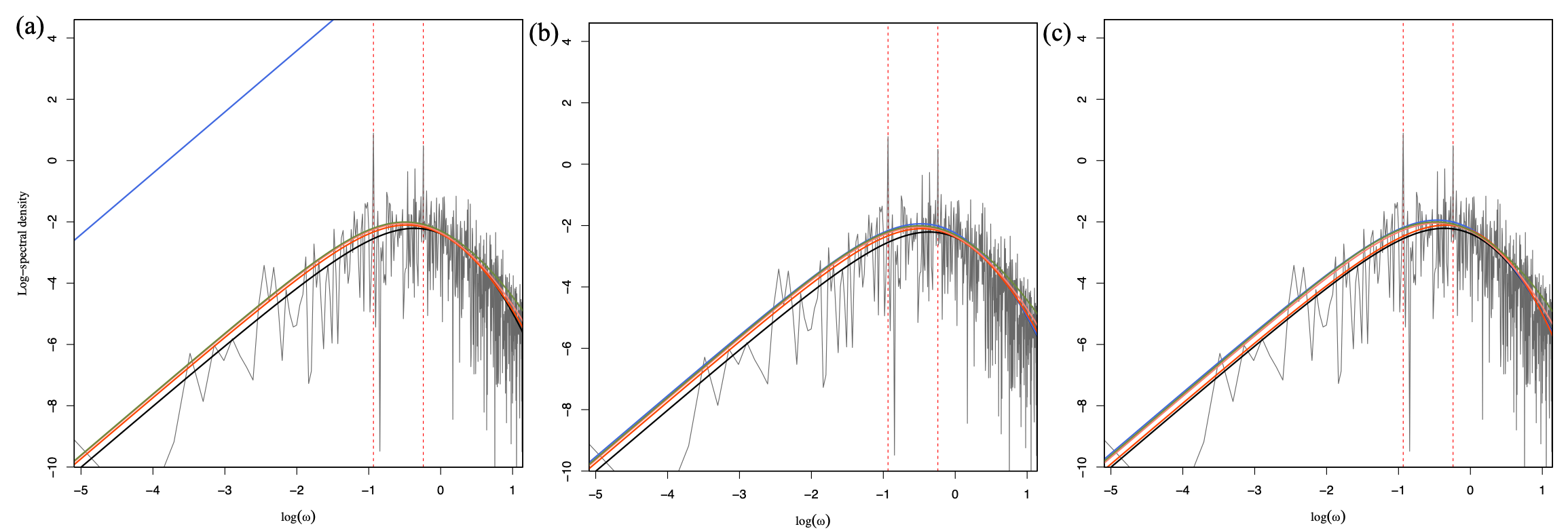
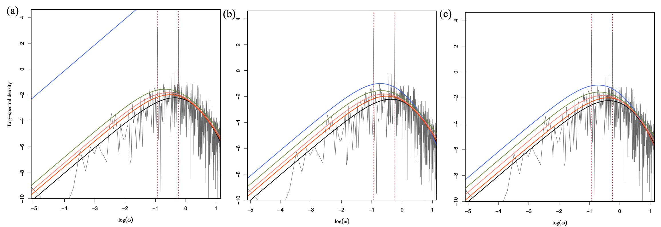
Figures 1 and 2 display the estimated spectral densities. In each figure, the following representations are used:

  • The solid gray curve represents the periodogram $I_{n}$;

  • the solid black curve denotes the true spectral density $S^{\mathrm{BA}}_{\theta^{*}}$;

  • the solid blue curve illustrates the spectral density with the minimum Itakura–Saito divergence estimate plugged-in;

  • the solid red, salmon pink, and green curves display the spectral densities with the minimum spectral Rényi divergence ($\alpha=0.9,0.75,0.5$) estimates plugged-in, respectively.

For any initial value and regardless of the existence of the trend, the spectral density based on the spectral $\alpha=0.5$-Rényi divergence aligns well with the true spectral density. The minimum spectral Rényi divergence estimate with any $\alpha\in\{0.5,0.75,0.9\}$ remains stable with respect to the choice of the initial value. Conversely, the minimum Itakura–Saito divergence estimate shows sensitivity to this choice.

Tables 1 and 2 summaries the estimation results. Comparing the results based on different initial values, we find that the minimum Itakura–Saito divergence estimates are sensitive to the initial value of the optimization regardless of the existence of the smoother, while the spectral Rényi divergence yields estimation results stable to the choice of the initial value. The minimum Itakura–Saito divergence estimate with the smoothed periodogram performs quite worser than that with the periodogram. In the presence of outliers in the frequency domain, the minimum Rényi divergence estimate with $\alpha=0.5$ performs the best regardless of the choice of the initial value in this example.

5 Discussions

The value of $\alpha$ controls the trade-off between the the efficiency without the presence of outliers and the robustness even for larger trends. For an objective selection of $\alpha$, constructing an information criterion is one possible direction, but requires sufficient discussions and experiments. In practice, monitoring the behaviours of the minimum spectral Rényi divergence estimates for several values of $\alpha$ (say, $\alpha=0.5,0.75,0.9$) would be a workaround.

Numerical experiments presented in Section 4 suggest that the minimum spectral Rényi divergence estimates are robust to the choice of an initial value, while the minimum Itakura–Saito divergence estimate is sensitive to it. These robustness and sensitivity are confirmed in the other examples such as autoregressive models. The structure of the gradient $\mathcal{G}_{\alpha}(\theta\,;\,\widetilde{I}_{n})$ in the comparison with that of $\mathcal{G}_{1}(\theta\,;\,\widetilde{I}_{n})$ can give a clue to this, and so detailed analysis of these gradient landscapes would be one of interesting research directions.

6 Acknowledgement

The authors would like to thank Akifumi Okuno, Mirai Tanaka, Kei Kobayashi, Yuta Koike, and Tomoyuki Higuchi for their comments. This work is supported by JSPS KAKENHI (19K20222, 21H05205, 21K12067, 23K11024), MEXT (JPJ010217), and “Strategic Research Projects” grant (2022-SRP-13) from ROIS (Research Organization of Information and Systems).

References

  • [1] P. Brockwell and R. Davis. Time Series: Theory and Methods. Springer, 2nd edition, 1991.
  • [2] J. Brune. Tectonic stress and spectra of seismic shear waves from earthquakes. Journal of Geophysical Research, 75:4997–5009, 1970.
  • [3] G. Calderoni and R. Abercrombie. Investigating spectral estimates of stress drop for small to moderate earthquakes with heterogeneous slip distribution: Examples from the 2016–2017 amatrice earthquake sequence. Journal of Geophysical Research: Solid Earth, 128, 2023.
  • [4] M. Gil, F. Alajaji, and T. Linder. Rényi divergence measures for commonly used univariate continuous distributions. Information Sciences, 249:124–131, 2013.
  • [5] E. Grivel, R. Diversi, and F. Merchan. Kullback–Leibler and Rényi divergence rate for Gaussian stationary ARMA processes comparison. Digital Signal Processing, 116:103089, 2021.
  • [6] C. Heyde and W. Dai. On the robustness to small trends of estimation based on the smoothed periodogram. Journal of Time Series Analysis, 17:141–150, 1996.
  • [7] F. Iacone. Local whittle estimation of the memory parameter in presence of deterministic components. Journal of Time Series Analysis, 31:37–49, 2010.
  • [8] F. Itakura and S. Saito. Analysis synthesis telephony based on the maximum likelihood method. Proceedings of the 6th of the International Congress on Acoustics, pages C17–C20, 1968.
  • [9] K. Aki K and P. Richards. Quantitative seismology: theory and methods. W H Freeman and Company, 1980.
  • [10] R. Martin. Statistical Methods for the Enhancement of Noisy Speech, chapter 2, pages 43–65. Springer Berlin/Heidelberg, 2005.
  • [11] B. Matérn. Spatial Variation: Stochastic Models and Their Application to Some Problems in Forest Surveys and Other Sampling Investigations. Stockholm: Statens Skogsforskningsinstitut, 1960.
  • [12] A. McCloskey and P. Perron. Memory parameter estimation in the presence of level shifts and deterministic trends. Econometric Theory, 29:1196–1237, 2013.
  • [13] E. Parzen. Stationary time series analysis using information and spectral analysis. In S. Rao and, editor, Developments in Time Series Analysis. In Honour of M. B. Priestley, pages 139––148. Chapman & Hall, 1993.
  • [14] M. Pinsker. Information and information stability of random variables and processes. Holden-Day, 1964. Translated and edited by A. Feinstein.
  • [15] P. Shayevitz. A note on a characterization of Rényi measures and its relation to composite hypothesis testing, 2010.
  • [16] M. Taniguchi. Minimum contrast estimation for spectral densities of stationary processes. Journal of the Royal Statistical Society. Series B, 49:315–325, 1987.
  • [17] I. Vajda. Theory of Statistical Inference and Information. Springer Dordrecht, 1989.
  • [18] T. van Erven and P. Harremos. Rényi divergence and Kullback–Leibler divergence. IEEE Transactions on Information Theory, 60:3797–3820, 2014.
  • [19] P. Whittle. The analysis of multiple stationary time series. Journal of the Royal Statistical Society. Series B (Methodological), 15:125–139, 1953.
  • [20] N. Yoshimitsu, T. Maeda, and T. Sei. Estimation of source parameters using a non-Gaussian probability density function in a bayesian framework. Earth, Planets and Space, 75, 2023.

Appendix A Proof of Proposition 2

Proof.

The difference between $\widehat{\theta}^{(1)}_{1}[\widetilde{I}^{z,\omega^{*}}_{n}]$ and $\widehat{\theta}^{(1)}_{1}[\widetilde{I}_{n}]$ is explicitly written as

$\displaystyle\|\widehat{\theta}^{(1)}_{1}[\widetilde{I}^{z,\omega^{*}}_{n}]-\widehat{\theta}^{(1)}_{1}[\widetilde{I}_{n}]\|$ $\displaystyle=\|\{\widehat{\theta}^{(1)}_{1}[\widetilde{I}^{z,\omega^{*}}_{n}]-\theta^{(0)}\}-\{\widehat{\theta}^{(1)}_{1}[\widetilde{I}_{n}]-\theta^{(0)}\}\|$
$\displaystyle=\frac{\gamma_{1}z}{n}\left\|\frac{\nabla_{\theta^{(0)}}\log S_{\theta}(\omega^{*})}{S_{\theta^{(0)}}(\omega^{*})}\right\|,$

which proves the first assertion. For the second assertion, observe

$\displaystyle\sum_{\omega\in\Omega_{n}}\left[1-\frac{\widetilde{I}^{z,\omega^{*}}_{n}(\omega)}{S_{\theta}(\omega)}\right]\nabla_{\theta}\log S_{\theta}(\omega)\Bigg{|}_{\theta=\widehat{\theta}^{(\infty)}_{1}[\widetilde{I}^{z,\omega^{*}}_{n}]}$
$\displaystyle=\sum_{\omega\in\Omega_{n}}\left[1-\frac{\widetilde{I}_{n}(\omega)}{S_{\theta}(\omega)}\right]\nabla_{\theta}\log S_{\theta}(\omega)\Bigg{|}_{\theta=\widehat{\theta}^{(\infty)}_{1}[\widetilde{I}^{z,\omega^{*}}_{n}]}-z\frac{\nabla_{\widehat{\theta}^{(\infty)}_{1}[\widetilde{I}^{z,\omega^{*}}_{n}]}\log S_{\theta}(\omega^{*})}{S_{\widehat{\theta}^{(\infty)}_{1}[\widetilde{I}^{z,\omega^{*}}_{n}]}(\omega^{*})}.$

This gives the second assertion, which completes the proof. ∎

Appendix B Proof of Theorem 3

Proof.

We prove Theorem 3 by the mathematical induction.

Step 1: Consider $m=1$. Observe

$\displaystyle\widehat{\theta}^{(1)}_{\alpha}[\widetilde{I}^{z,\omega^{*}}_{n}]-\widehat{\theta}^{(1)}_{\alpha}[\widetilde{I}_{n}]$
$\displaystyle=\left\{\widehat{\theta}^{(1)}_{\alpha}[\widetilde{I}^{z,\omega^{*}}_{n}]-\theta^{(0)}\right\}-\left\{\widehat{\theta}^{(1)}_{\alpha}[\widetilde{I}_{n}]-\theta^{(0)}\right\}$
$\displaystyle=\frac{\gamma_{1}\alpha}{(1-\alpha)n}\left(\frac{S_{\theta^{(0)}}(\omega^{*})}{\alpha S_{\theta^{(0)}}(\omega^{*})+(1-\alpha)\widetilde{I}_{n}(\omega^{*})}-\frac{S_{\theta^{(0)}}(\omega^{*})}{\alpha S_{\theta^{(0)}}(\omega^{*})+(1-\alpha)(\widetilde{I}_{n}(\omega^{*})+z)}\right)\nabla_{\theta^{(0)}}\log S_{\theta}(\omega^{*})$
$\displaystyle=\frac{\gamma_{1}}{(1-\alpha)n}\frac{\alpha S_{\theta^{(0)}}(\omega^{*})}{\alpha S_{\theta^{(0)}}(\omega^{*})+(1-\alpha)\widetilde{I}_{n}(\omega^{*})}\frac{(1-\alpha)z\nabla_{\theta^{(0)}}S_{\theta}(\omega^{*})}{(1-\alpha)z+(1-\alpha)\widetilde{I}_{n}(\omega^{*})+\alpha S_{\theta^{(0)}}(\omega^{*})}.$

This yields

$\displaystyle\left\|\widehat{\theta}^{(1)}_{\alpha}[\widetilde{I}^{z,\omega^{*}}_{n}]-\widehat{\theta}^{(1)}_{\alpha}[\widetilde{I}_{n}]\right\|\leq\frac{1}{n}\frac{\gamma_{1}}{1-\alpha}\|\nabla_{\theta^{(0)}}S_{\theta}(\omega^{*})\|,$

which proves the assertion for $m=1$.

Step 2: Let $m\in\mathbb{N}>1$. Assume that for any $\varepsilon>0$, there exists $N\in\mathbb{N}$ such that for $n\geq N$, we have

$\displaystyle\|\widehat{\theta}^{(m)}_{\alpha}[\widetilde{I}_{n}^{z,\omega^{*}}]-\widehat{\theta}^{(m)}_{\alpha}[\widetilde{I}_{n}]\|\leq\varepsilon.$

By the cancelling technique and by the triangle inequality, we get

$\displaystyle\left\|\widehat{\theta}^{(m+1)}_{\alpha}[\widetilde{I}_{n}^{z,\omega^{*}}]-\widehat{\theta}^{(m+1)}_{\alpha}[\widetilde{I}_{n}]\right\|$
$\displaystyle=\left\|\left\{\widehat{\theta}^{(m+1)}_{\alpha}[\widetilde{I}_{n}^{z,\omega^{*}}]-\widehat{\theta}^{(m)}_{\alpha}[\widetilde{I}_{n}^{z,\omega^{*}}]\right\}-\left\{\widehat{\theta}^{(m+1)}_{\alpha}[\widetilde{I}_{n}]-\widehat{\theta}^{(m)}_{\alpha}[\widetilde{I}_{n}]\right\}-\left\{\widehat{\theta}^{(m)}_{\alpha}[\widetilde{I}_{n}^{z,\omega^{*}}]-\widehat{\theta}^{(m)}_{\alpha}[\widetilde{I}_{n}]\right\}\right\|$
$\displaystyle\leq\left\|\mathcal{G}_{\alpha}\left(\widehat{\theta}^{(m)}_{\alpha}[\widetilde{I}^{z,\omega^{*}}_{n}]\,;\,\widetilde{I}^{z,\omega^{*}}_{n}\right)-\mathcal{G}_{\alpha}\left(\widehat{\theta}^{(m)}_{\alpha}[\widetilde{I}_{n}]\,;\,\widetilde{I}_{n}\right)\right\|+\varepsilon.$

Observe that by applying the Taylor theorem to $\nabla_{\theta}\log S_{\theta}(\omega)$ and letting $t$ be some point on some line connecting $\widehat{\theta}^{(m)}_{\alpha}[\widetilde{I}^{z,\omega^{*}}_{n}]$ to $\widehat{\theta}^{(m)}_{\alpha}[\widetilde{I}_{n}]$, we get

$\displaystyle\mathcal{G}_{\alpha}\left(\widehat{\theta}^{(m)}_{\alpha}[\widetilde{I}^{z,\omega^{*}}_{n}]\,;\,\widetilde{I}^{z,\omega^{*}}_{n}\right)$
$\displaystyle=\frac{\gamma_{m}\alpha}{(1-\alpha)n}\sum_{\omega\in\Omega_{n}}\left\{1-\frac{S_{\widehat{\theta}^{(m)}_{\alpha}[\widetilde{I}^{z,\omega^{*}}_{n}]}(\omega)}{\alpha S_{\widehat{\theta}^{(m)}_{\alpha}[\widetilde{I}^{z,\omega^{*}}_{n}]}(\omega)+(1-\alpha)\widetilde{I}^{z,\omega^{*}}_{n}(\omega)}\right\}\nabla_{\widehat{\theta}^{(m)}_{\alpha}[\widetilde{I}^{z,\omega^{*}}_{n}]}\log S_{\theta}(\omega)$
$\displaystyle=\frac{\gamma_{m}\alpha}{(1-\alpha)n}\sum_{\omega\in\Omega_{n}}\left\{1-\frac{S_{\widehat{\theta}^{(m)}_{\alpha}[\widetilde{I}^{z,\omega^{*}}_{n}]}(\omega)}{\alpha S_{\widehat{\theta}^{(m)}_{\alpha}[\widetilde{I}^{z,\omega^{*}}_{n}]}(\omega)+(1-\alpha)\widetilde{I}^{z,\omega^{*}}_{n}(\omega)}\right\}\nabla_{\widehat{\theta}^{(m)}_{\alpha}[\widetilde{I}_{n}]}\log S_{\theta}(\omega)$
$\displaystyle\quad+\frac{\gamma_{m}\alpha}{(1-\alpha)n}\sum_{\omega\in\Omega_{n}}\left\{1-\frac{S_{\widehat{\theta}^{(m)}_{\alpha}[\widetilde{I}^{z,\omega^{*}}_{n}]}(\omega)}{\alpha S_{\widehat{\theta}^{(m)}_{\alpha}[\widetilde{I}^{z,\omega^{*}}_{n}]}(\omega)+(1-\alpha)\widetilde{I}^{z,\omega^{*}}_{n}(\omega)}\right\}\nabla_{t}^{2}\log S_{\theta}(\omega)(\widehat{\theta}^{(m)}_{\alpha}[\widetilde{I}^{z,\omega^{*}}_{n}]-\widehat{\theta}^{(m)}_{\alpha}[\widetilde{I}])$
$\displaystyle=\frac{\gamma_{m}\alpha}{(1-\alpha)n}\sum_{\omega\in\Omega_{n}}\left\{1-\frac{S_{\widehat{\theta}^{(m)}_{\alpha}[\widetilde{I}^{z,\omega^{*}}_{n}]}(\omega)}{\alpha S_{\widehat{\theta}^{(m)}_{\alpha}[\widetilde{I}^{z,\omega^{*}}_{n}]}(\omega)+(1-\alpha)\widetilde{I}^{z,\omega^{*}}_{n}(\omega)}\right\}\nabla_{\widehat{\theta}^{(m)}_{\alpha}[\widetilde{I}_{n}]}\log S_{\theta}(\omega)$
$\displaystyle\quad+O\left(\frac{2\gamma_{m}\varepsilon}{(1-\alpha)n}\sup_{\theta\in\Theta}\sum_{\omega\in\Omega_{n}}\|\nabla^{2}_{\theta}\log S_{\theta}(\omega)\|_{\mathrm{op}}\right),$

where $O(1)$ in the rightmost side implies a vector whose norm is $O(1)$. This yields

$\displaystyle\mathcal{G}_{\alpha}\left(\widehat{\theta}^{(m)}_{\alpha}[\widetilde{I}^{z,\omega^{*}}_{n}]\,;\,\widetilde{I}^{z,\omega^{*}}_{n}\right)-\mathcal{G}_{\alpha}\left(\widehat{\theta}^{(m)}_{\alpha}[\widetilde{I}_{n}]\,;\,\widetilde{I}_{n}\right)$
$\displaystyle=\frac{\gamma_{m}\alpha}{(1-\alpha)n}\sum_{\omega\in\Omega_{n}}\left\{\frac{S_{\widehat{\theta}^{(m)}_{\alpha}[\widetilde{I}_{n}]}(\omega)}{\alpha S_{\widehat{\theta}^{(m)}_{\alpha}[\widetilde{I}_{n}]}(\omega)+(1-\alpha)\widetilde{I}_{n}(\omega)}-\frac{S_{\widehat{\theta}^{(m)}_{\alpha}[\widetilde{I}^{z,\omega^{*}}_{n}]}(\omega)}{\alpha S_{\widehat{\theta}^{(m)}_{\alpha}[\widetilde{I}^{z,\omega^{*}}_{n}]}(\omega)+(1-\alpha)\widetilde{I}^{z,\omega^{*}}_{n}(\omega)}\right\}$
$\displaystyle\qquad\qquad\quad\qquad\qquad\nabla_{\widehat{\theta}^{(m)}_{\alpha}[\widetilde{I}_{n}]}\log S_{\theta}(\omega)$
$\displaystyle\quad+O\left(\frac{2\gamma_{m}\varepsilon}{(1-\alpha)n}\sup_{\theta\in\Theta}\sum_{\omega\in\Omega_{n}}\|\nabla^{2}_{\theta}\log S_{\theta}(\omega)\|_{\mathrm{op}}\right)$
$\displaystyle=\frac{\gamma_{m}\alpha}{(1-\alpha)n}\sum_{\omega\in\Omega_{n}}\left\{\frac{S_{\widehat{\theta}^{(m)}_{\alpha}[\widetilde{I}_{n}]}(\omega)}{\alpha S_{\widehat{\theta}^{(m)}_{\alpha}[\widetilde{I}_{n}]}(\omega)+(1-\alpha)\widetilde{I}_{n}(\omega)}-\frac{S_{\widehat{\theta}^{(m)}_{\alpha}[\widetilde{I}_{n}]}(\omega)}{\alpha S_{\widehat{\theta}^{(m)}_{\alpha}[\widetilde{I}_{n}]}(\omega)+(1-\alpha)\widetilde{I}^{z,\omega^{*}}_{n}(\omega)}\right.$
$\displaystyle\left.\qquad\qquad\quad\qquad\qquad+\frac{S_{\widehat{\theta}^{(m)}_{\alpha}[\widetilde{I}_{n}]}(\omega)}{\alpha S_{\widehat{\theta}^{(m)}_{\alpha}[\widetilde{I}_{n}]}(\omega)+(1-\alpha)\widetilde{I}^{z,\omega^{*}}_{n}(\omega)}-\frac{S_{\widehat{\theta}^{(m)}_{\alpha}[\widetilde{I}^{z,\omega^{*}}_{n}]}(\omega)}{\alpha S_{\widehat{\theta}^{(m)}_{\alpha}[\widetilde{I}^{z,\omega^{*}}_{n}]}(\omega)+(1-\alpha)\widetilde{I}^{z,\omega^{*}}_{n}(\omega)}\right\}$
$\displaystyle\qquad\qquad\quad\qquad\qquad\nabla_{\widehat{\theta}^{(m)}_{\alpha}[\widetilde{I}_{n}]}\log S_{\theta}(\omega)$
$\displaystyle\quad+O\left(\frac{2\gamma_{m}\varepsilon}{(1-\alpha)n}\sup_{\theta\in\Theta}\sum_{\omega\in\Omega_{n}}\|\nabla^{2}_{\theta}\log S_{\theta}(\omega)\|_{\mathrm{op}}\right)$
$\displaystyle=\frac{\gamma_{m}\alpha}{(1-\alpha)n}(T_{1}+T_{2})+O\left(\frac{2\gamma_{m}\varepsilon}{(1-\alpha)n}\sup_{\theta\in\Theta}\sum_{\omega\in\Omega_{n}}\|\nabla^{2}_{\theta}\log S_{\theta}(\omega)\|_{\mathrm{op}}\right),$

where

$\displaystyle T_{1}$ $\displaystyle:=\sum_{\omega\in\Omega_{n}}\left\{\frac{S_{\widehat{\theta}^{(m)}_{\alpha}[\widetilde{I}_{n}]}(\omega)}{\alpha S_{\widehat{\theta}^{(m)}_{\alpha}[\widetilde{I}_{n}]}(\omega)+(1-\alpha)\widetilde{I}_{n}(\omega)}-\frac{S_{\widehat{\theta}^{(m)}_{\alpha}[\widetilde{I}_{n}]}(\omega)}{\alpha S_{\widehat{\theta}^{(m)}_{\alpha}[\widetilde{I}_{n}]}(\omega)+(1-\alpha)\widetilde{I}^{z,\omega^{*}}_{n}(\omega)}\right\}\nabla_{\widehat{\theta}^{(m)}_{\alpha}[\widetilde{I}_{n}]}\log S_{\theta}(\omega),$
$\displaystyle T_{2}$ $\displaystyle:=\sum_{\omega\in\Omega_{n}}\left\{\frac{S_{\widehat{\theta}^{(m)}_{\alpha}[\widetilde{I}_{n}]}(\omega)}{\alpha S_{\widehat{\theta}^{(m)}_{\alpha}[\widetilde{I}_{n}]}(\omega)+(1-\alpha)\widetilde{I}^{z,\omega^{*}}_{n}(\omega)}-\frac{S_{\widehat{\theta}^{(m)}_{\alpha}[\widetilde{I}^{z,\omega^{*}}_{n}]}(\omega)}{\alpha S_{\widehat{\theta}^{(m)}_{\alpha}[\widetilde{I}^{z,\omega^{*}}_{n}]}(\omega)+(1-\alpha)\widetilde{I}^{z,\omega^{*}}_{n}(\omega)}\right\}$
$\displaystyle\qquad\qquad\quad\nabla_{\widehat{\theta}^{(m)}_{\alpha}[\widetilde{I}_{n}]}\log S_{\theta}(\omega).$

Here we have

$\displaystyle T_{1}$ $\displaystyle=\frac{\alpha S_{\widehat{\theta}^{(m)}_{\alpha}[\widetilde{I}_{n}]}(\omega^{*})}{\alpha S_{\widehat{\theta}^{(m)}_{\alpha}[\widetilde{I}_{n}]}(\omega^{*})+(1-\alpha)\widetilde{I}_{n}(\omega^{*})}\frac{(1-\alpha)z}{(1-\alpha)z+\alpha S_{\widehat{\theta}^{(m)}_{\alpha}[\widetilde{I}_{n}]}(\omega^{*})+(1-\alpha)\widetilde{I}_{n}(\omega^{*})}\frac{\nabla_{\widehat{\theta}^{(m)}_{\alpha}[\widetilde{I}_{n}]}\log S_{\theta}(\omega^{*})}{\alpha}$
$\displaystyle=O\left(\frac{1}{\alpha}\sup_{\theta,\,\omega}\|\nabla_{\theta}\log S_{\theta}(\omega)\|\right)$

and

$\displaystyle T_{2}$ $\displaystyle=\sum_{\omega\in\Omega_{n}}\frac{(1-\alpha)\widetilde{I}^{z,\omega^{*}}_{n}(\omega)}{\alpha S_{\widehat{\theta}^{(m)}_{\alpha}[\widetilde{I}^{z,\omega^{*}}_{n}]}(\omega)+(1-\alpha)\widetilde{I}^{z,\omega^{*}}_{n}(\omega)}\frac{S_{\widehat{\theta}^{(m)}_{\alpha}[\widetilde{I}_{n}]}(\omega)-S_{\widehat{\theta}^{(m)}_{\alpha}[\widetilde{I}^{z,\omega^{*}}_{n}]}(\omega)}{\alpha S_{\widehat{\theta}^{(m)}_{\alpha}[\widetilde{I}_{n}]}(\omega)+(1-\alpha)\widetilde{I}^{z,\omega^{*}}_{n}(\omega)}\nabla_{\widehat{\theta}^{(m)}_{\alpha}[\widetilde{I}_{n}]}\log S_{\theta}(\omega)$
$\displaystyle=O\left(\frac{n\varepsilon}{\alpha}\sup_{\theta,\theta^{\prime},\omega}\|\nabla_{\theta^{\prime}}S_{\theta}(\omega)\|\|(1/S_{\theta}(\omega))\nabla_{\theta}\log S_{\theta}(\omega)\|\right).$

Then we obtain

$\displaystyle\left\|\mathcal{G}_{\alpha}\left(\widehat{\theta}^{(m)}_{\alpha}[\widetilde{I}^{z,\omega^{*}}_{n}]\,;\,\widetilde{I}^{z,\omega^{*}}_{n}\right)-\mathcal{G}_{\alpha}\left(\widehat{\theta}^{(m)}_{\alpha}[\widetilde{I}_{n}]\,;\,\widetilde{I}_{n}\right)\right\|$
$\displaystyle\leq\frac{\gamma_{m}}{(1-\alpha)n}\sup_{\theta,\omega}\|\nabla_{\theta}\log S_{\theta}(\omega)\|$
$\displaystyle\quad+\varepsilon\left\{\frac{\gamma_{m}}{(1-\alpha)}\left(\sup_{\theta,\omega}\|\nabla_{\theta,\omega}S_{\theta}(\omega)\|\right)^{2}+\frac{2\gamma_{m}}{(1-\alpha)}\sup_{\theta\in\Theta}\frac{1}{n}\sum_{\omega\in\Omega_{n}}\|\nabla^{2}_{\theta}\log S_{\theta}(\omega)\|_{\mathrm{op}}\right\}$

and thus

$\displaystyle\left\|\widehat{\theta}^{(m+1)}_{\alpha}[\widetilde{I}_{n}^{z,\omega^{*}}]-\widehat{\theta}^{(m+1)}_{\alpha}[\widetilde{I}_{n}]\right\|$
$\displaystyle\leq\frac{\gamma_{m}}{(1-\alpha)n}\sup_{\theta,\omega}\|\nabla_{\theta}\log S_{\theta}(\omega)\|$
$\displaystyle\quad+\varepsilon\left\{1+\frac{\gamma_{m}}{(1-\alpha)}\left(\sup_{\theta,\omega}\|\nabla_{\theta,\omega}S_{\theta}(\omega)\|\right)^{2}+\frac{2\gamma_{m}}{(1-\alpha)}\sup_{\theta\in\Theta}\frac{1}{n}\sum_{\omega\in\Omega_{n}}\|\nabla^{2}_{\theta}\log S_{\theta}(\omega)\|_{\mathrm{op}}\right\}.$

This implies that the assertion holds for $m+1$ and by the mathematical induction, we get the conclusion. ∎

Appendix C Additional simulation studies

This appendix presents additional numerical experiments.

Tables 3 and 4 show the estimation results for the Brune spectral model with attenuation in Section 4.1 on the basis of the different initial values $\theta^{(0),4}=(0.1,0.1,0.1)$ and $\theta^{(0),5}=(2,2,2)$. For almost all the settings of initial values, the spectral density based on the spectral $\alpha=0.5$-Rényi divergence performs the best.

Table 3: The mean values of biases with standard deviations without any trend. For each initial value, the values closest to zero are underlined.
Initial value $\widehat{\sigma}-\sigma^{*}$ $\widehat{\omega_{c}}-\omega_{c}^{*}$ $\widehat{Q}-Q^{*}$
Rényi ($\alpha=0.50$) $\theta^{(0),4}$ -0.03 ($\pm$0.05) -0.11 ($\pm$0.07) 0.26 ($\pm$0.15)
Rényi ($\alpha=0.75$) $\theta^{(0),4}$ 0.04 ($\pm$0.06) -0.30 ($\pm$0.03) 1.33 ($\pm$0.17)
Rényi ($\alpha=0.90$) $\theta^{(0),4}$ 0.09 ($\pm$0.08) -0.39 ($\pm$0.03) 6.13 ($\pm$0.04)
Itakura–Saito with $I_{n}$ $\theta^{(0),4}$ $5\cdot 10^{15}$ ($\pm 8\cdot 10^{14}$) $1\cdot 10^{16}$ ($\pm 1\cdot 10^{15}$) $8\cdot 10^{16}$ ($\pm 1\cdot 10^{16}$)
Itakura–Saito with $I_{n}^{S}$ $\theta^{(0),4}$ $5\cdot 10^{18}$ ($\pm 9\cdot 10^{18}$) $1\cdot 10^{19}$ ($\pm 1\cdot 10^{19}$) $9\cdot 10^{19}$ ($\pm 1\cdot 10^{20}$)
Rényi ($\alpha=0.50$) $\theta^{(0),5}$ -0.01($\pm$0.06) -0.18 ($\pm$0.05) 0.47 ($\pm$0.16)
Rényi ($\alpha=0.75$) $\theta^{(0),5}$ 0.01 ($\pm$ 0.06) -0.21 ($\pm$0.05) 0.68 ($\pm$0.22)
Rényi ($\alpha=0.90$) $\theta^{(0),5}$ 0.02 ($\pm$0.06) -0.24 ($\pm$0.04) 1.18 ($\pm$0.34)
Itakura–Saito with $I_{n}$ $\theta^{(0),5}$ 0.07 ($\pm$0.11) -0.08 ($\pm$0.12) 0.12 ($\pm$0.18)
Itakura–Saito with $I_{n}^{S}$ $\theta^{(0),5}$ -0.28 ($\pm$0.16) 1.84 ($\pm$1.66) 1.90 ($\pm$0.63)
Table 4: The mean values of biases with standard deviations with the trigonometric trends. For each initial value, the values closest to zero are underlined.
Initial value $\widehat{\sigma}-\sigma^{*}$ $\widehat{\omega_{c}}-\omega_{c}^{*}$ $\widehat{Q}-Q^{*}$
Rényi ($\alpha=0.50$) $\theta^{(0),4}$ 0.21 ($\pm$0.07) -0.21 ($\pm$0.06) 0.24 ($\pm$0.14)
Rényi ($\alpha=0.75$) $\theta^{(0),4}$ 0.61 ($\pm$0.09) -0.43 ($\pm$0.02) 1.14 ($\pm$0.20)
Rényi ($\alpha=0.90$) $\theta^{(0),4}$ 1.65 ($\pm$0.12) -0.60 ($\pm$0.02) 6.05 ($\pm$0.05)
Itakura–Saito with $I_{n}$ $\theta^{(0),4}$ $5\cdot 10^{15}$ ($\pm 8\cdot 10^{14}$) $1\cdot 10^{16}$ ($\pm 1\cdot 10^{15}$) $8\cdot 10^{16}$ ($\pm 1\cdot 10^{16}$)
Itakura–Saito with $I_{n}^{S}$ $\theta^{(0),4}$ $5\cdot 10^{18}$ ($\pm 9\cdot 10^{18}$) $1\cdot 10^{19}$ ($\pm 1\cdot 10^{19}$) $9\cdot 10^{19}$ ($\pm 1\cdot 10^{20}$)
Rényi ($\alpha=0.50$) $\theta^{(0),5}$ 0.23 ($\pm$0.07) -0.26 ($\pm$0.04) 0.41 ($\pm$0.16)
Rényi ($\alpha=0.75$) $\theta^{(0),5}$ 0.55 ($\pm$0.08) -0.35 ($\pm$0.04) 0.55 ($\pm$0.20)
Rényi ($\alpha=0.90$) $\theta^{(0),5}$ 1.50 ($\pm$0.10) -0.50 ($\pm$0.03) 0.85 ($\pm$0.35)
Itakura–Saito with $I_{n}$ $\theta^{(0),5}$ 3.91 ($\pm$0.07) -0.34 ($\pm$0.02) -0.40 ($\pm$0.02)
Itakura–Saito with $I_{n}^{S}$ $\theta^{(0),5}$ 2.85 ($\pm$0.95) -0.17 ($\pm$0.51) 2.26 ($\pm$0.93)

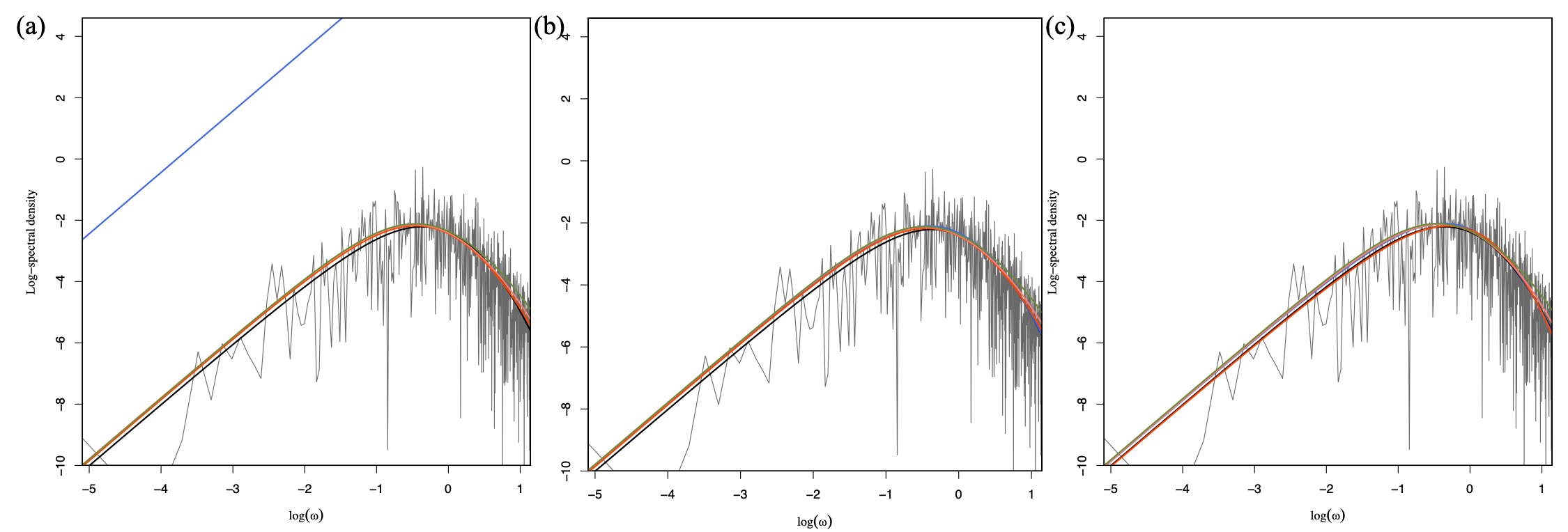
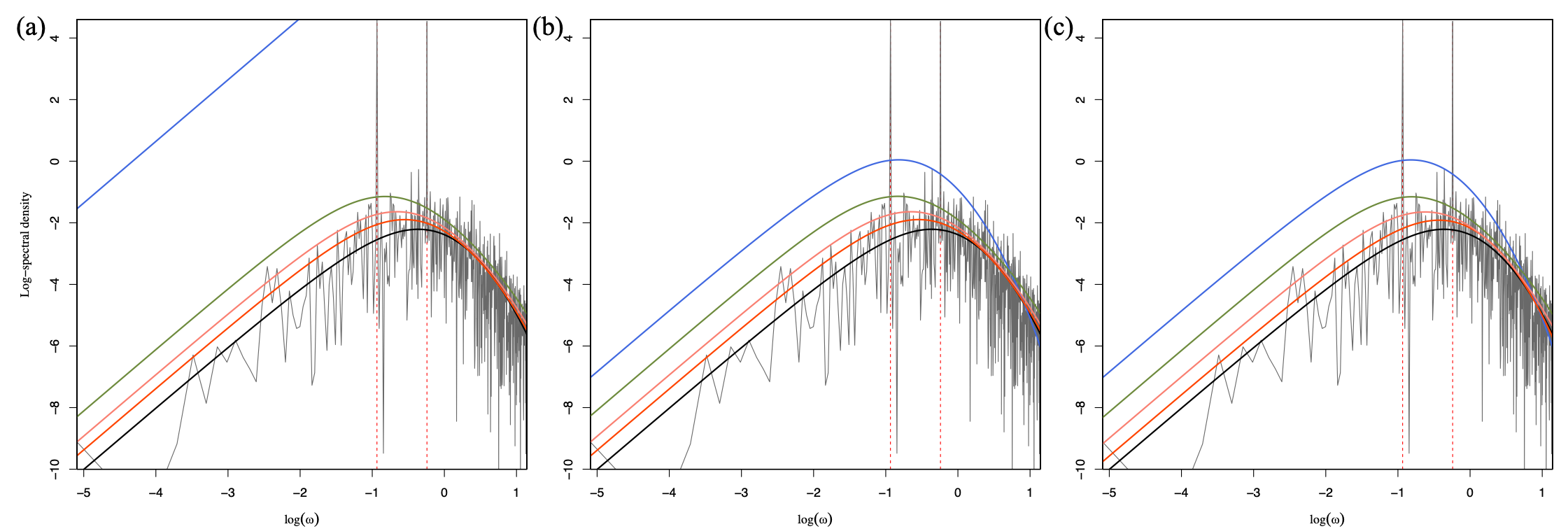
Figures 3 and 4 display an instance of a set of the estimated spectral densities. In each figure, the following representations are used:

  • The solid gray curve represents the periodogram $I_{n}$;

  • the solid black curve denotes the true spectral density $S^{\mathrm{BA}}_{\theta^{*}}$;

  • the solid blue curve illustrates the spectral density with the minimum Itakura–Saito divergence estimate plugged-in;

  • the solid red, salmon pink, and green curves display the spectral density with the minimum spectral Rényi divergence ($\alpha=0.9,0.75,0.5$) estimates plugged-in, respectively.

For any initial value and for any strength of trends, the spectral density based on the spectral $\alpha=0.5$-Rényi divergence performs the best.

Refer to caption
Figure 3: Spectral densities with the estimates plugged-in for the Brune spectral model with attenuation and with the trigonometric trends of $z_{1}=z_{2}=2.5$. The gray curve is the periodogram. The true spectral density is colored in black. Spectral densities based on the spectral Rényi divergence ($\alpha=0.5,0.75,0.9$) are colored in red, salmon pink, and green,respectively. The spectral density based on the Itakura–Saito divergence is colored in blue. The red dashed lines denote the frequencies at which the outliers are injected. (a) the result based on the initial value $\theta^{(0),1}$, (b) the result based on the initial value $\theta^{(0),2}$, (c) the result based on the initial value $\theta^{(0),3}$.
Refer to caption
Figure 4: Spectral densities with the estimates plugged-in for the Brune spectral model with attenuation and with the trigonometric trends of $z_{1}=z_{2}=25$. The gray curve is the periodogram. The true spectral density is colored in black. Spectral densities based on the spectral Rényi divergence ($\alpha=0.5,0.75,0.9$) are colored in red, salmon pink, and green,respectively. The spectral density based on the Itakura–Saito divergence is colored in blue. The red dashed lines denote the frequencies at which the outliers are injected. (a) the result based on the initial value $\theta^{(0),1}$, (b) the result based on the initial value $\theta^{(0),2}$, (c) the result based on the initial value $\theta^{(0),3}$.