Non-stationary elastic wave scattering and energy transport in a one-dimensional harmonic chain with an isotopic defect

Abstract

The fundamental solution describing non-stationary elastic wave scattering on an isotopic defect in a one-dimensional harmonic chain is obtained in an asymptotic form. The chain is subjected to unit impulse point loading applied to a particle far enough from the defect. The solution is a large time asymptotics at a moving point of observation, and it is in excellent agreement with the corresponding numerical calculations. At the next step, we assume that the applied point impulse excitation has random amplitude. This allows one to model the heat transport in the chain and across the defect as the transport of the mathematical expectation for the kinetic energy and to use the conception of the kinetic temperature. To provide a simplified continuum description for this process, we separate the slow in time component of the kinetic temperature. This quantity can be calculated using the asymptotics of the fundamental solution for the deterministic problem. We demonstrate that there is a thermal shadow behind the defect: the order of vanishing for the slow temperature is larger for the particles behind the defect than for the particles between the loading and the defect. The presence of the thermal shadow is related to a non-stationary wave phenomenon, which we call the anti-localization of non-stationary waves. Due to the presence of the shadow, the continuum slow kinetic temperature has a jump discontinuity at the defect. Thus, the system under consideration can be a simple model for the non-stationary phenomenon, analogous to one characterized by the Kapitza thermal resistance. Finally, we analytically calculate the non-stationary transmission function, which describes the distortion (caused by the defect) of the slow kinetic temperature profile at a far zone behind the defect.

1 Introduction

We consider the non-stationary dynamics of a one-dimensional harmonic crystal (a linear chain) with an isotopic defect subjected to a point impulse loading applied outside (more precisely, far enough) of the defect. The present paper is a natural continuation of our previous paper Shishkina and Gavrilov (2023), where we considered the same system but with the loading applied at the defect. Now, the alternated mathematical formulation corresponds to the essentially different physical nature of the dynamical processes in the chain. Namely, we deal with the problem of non-stationary scattering (or non-stationary diffraction) of an elastic quasi-wave on a point defect. We speak about a quasi-wave since the perturbations in discrete systems propagate at infinite speed. In what follows, we often refer to quasi-waves as waves. On the other hand, the problem concerning non-stationary scattering is essentially more difficult from a mathematical point of view compared with the one considered in Shishkina and Gavrilov (2023). The practical motivation for our study is experimental observations (see, e.g., Chen et al. (2012)), which indicate that the presence of isotopic defects essentially affects the thermal conductivity of pure nanomaterials.

An extensive bibliography on the studies, which deal with a chain with an isotopic defect, can be found in our previous paper Shishkina and Gavrilov (2023). Many of them consider the case when the loading (deterministic or stochastic) is applied at the defect Teramoto and Takeno (1960); Kashiwamura (1962); Hemmer (1959); Magalinskii (1959); Müller (1962); Müller and Weiss (2012); Turner (1960); Rubin (1960, 1961, 1963); Lee et al. (1989); Yu (2019). In Takizawa and Kobayasi (1968a, b), the general solution is obtained, which involves both cases when the loading is applied on or outside the defect, but it has a complicated form and is difficult for analysis. In Kannan (2013); Paul and Gendelman (2020); Gendelman and Paul (2021); Plyukhin (2020), the steady-state problem concerning the thermal conductivity of a chain of a finite length with an isotopic defect subjected to thermal (stochastic) sources at the ends is considered. The scattering problem was considered mostly in the stationary statement Koster (1954); Lifšic (1956); Fellay et al. (1997); Kosevich (2008, 1997); Kossevich (1999); Lifshitz and Kosevich (1966). In particular, the stationary three-dimensional problems concerning the scattering on a point or a two-dimensional (plane) defect are discussed in Kossevich (1999); Lifshitz and Kosevich (1966). In Fellay et al. (1997); Kosevich (2008, 1997), one-dimensional problems concerning scattering in a chain with a defect of a complex structure, where multichannel propagation is possible, are considered in the stationary statement. The similar, from a mathematical point of view, problem concerning a chain with an interface is discussed in the stationary formulation in Jex (1986); Kakodkar and Feser (2015); Kuzkin (2023); Lumpkin et al. (1978); Polanco et al. (2013); Saltonstall et al. (2013); Steinbrüchel (1976). Note that in physics, the phenomenon discussed in the framework of stationary problems is often referred to as phonon scattering Kakodkar and Feser (2015); Kosevich (2008); Steinbrüchel (1976); Saito et al. (2018). The incident wave is generally taken as an infinite harmonic plane wave, i.e., a phonon, not a harmonic wave corresponding to a point harmonic load. The stationary solution for a semi-infinite chain harmonically excited at the free end with an isotopic defect at an arbitrary position is obtained in Mokole et al. (1990).

In the current paper, as well as in Shishkina and Gavrilov (2023), we consider two problems: a deterministic and a stochastic one. We initially formulate the scattering problem as a deterministic problem (Sect. 3.1). Since a unit impulse point load is under consideration, the obtained solution can be treated as the fundamental one. Since the main point of interest in the paper is related to the stochastic kinetic energy (heat) transport problem, we are interested in the derivation of the fundamental solution for the particle velocities. In the framework of the stochastic problem (Sect. 3.2), we assume that the applied point impulse excitation has a random amplitude. This allows one to model the heat transport in the chain and across the defect as the transport of the mathematical expectation of the kinetic energy and to use the conception of the kinetic temperature. The propagation of the kinetic temperature is referred to in the paper as the thermal motions. The non-stationary fundamental solution, which describes this process, is the thermal fundamental solution.

Due to the linearity of the problem, the solution of the scattering problem can be represented as a superposition of an incident wave, which corresponds to the same loading in the uniform chain, and a scattered wave. The corresponding decomposition for the Green functions in the frequency domain is obtained in Sect. 4. In Sect. 5, we obtain the asymptotic solutions, which describe the non-stationary scattered wave and the total wave-field. The obtained solutions provide a continuum description of the wave-field and are in excellent agreement with the corresponding numerical calculations. The non-stationary solution for the scattered wave-field is found as a large time asymptotics at a moving point of observation, using a technique analogous to one used in our previous studies Shishkina et al. (2023); Shishkina and Gavrilov (2023); Gavrilov (2022).

In Sect. 6, we start to deal with the energy (heat) transport problem. Following the procedure suggested in Gavrilov (2022), we use the asymptotics of the fundamental solution for the deterministic problem and get slow and fast decoupling of the thermal fundamental solution. The slow motion (the slow component of the kinetic temperature) is introduced as the time average of the kinetic temperature over fast phases (time-like variables). Note that initially, the slow motion was introduced Krivtsov (2015); Kuzkin and Krivtsov (2017) as a formal solution of equations for covariances with dropped high-order time derivatives. The slow motion provides a simplified continuum description for the heat transport process. The fast motion is the energy oscillation related to the transformation of kinetic energy into potential energy and back Gavrilov and Krivtsov (2019); Krivtsov (2014); Kuzkin and Krivtsov (2017). In discrete harmonic systems, where a stochastic loading is distributed in space Krivtsov (2015, 2019); Sokolov et al. (2021); Kuzkin and Krivtsov (2017); Kuzkin (2019) or in time Gavrilov et al. (2019); Gavrilov and Krivtsov (2022, 2020), according to numerical calculations, the fast motion vanishes. Thus, we expect that to describe heat transport for such a loading, it is enough to calculate the convolution of the loading with the fundamental solution for the slow motion obtained in the paper (without any spatial or temporal averaging).

In Sect. 7, we demonstrate that there is a thermal shadow behind the defect: the order of vanishing for the slow temperature is larger for the particles behind the defect than for the particles between the loading and the defect. The presence of the thermal shadow is related to a non-stationary wave phenomenon, which we call the anti-localization of non-stationary waves Shishkina and Gavrilov (2023); Shishkina et al. (2023); Gavrilov et al. (2023). Due to the presence of the shadow, the continuum slow kinetic temperature has a jump discontinuity at the defect. Thus, we have shown that the system under consideration can be a simple model for the non-stationary phenomenon analogous to one characterized by the Kapitza (interfacial) thermal resistance Gendelman and Paul (2021); Kapitza (1941); Lumpkin et al. (1978); Paul and Gendelman (2020). Finally, we analytically calculate the non-stationary transmission function, which describes the distortion (caused by the defect) of the slow kinetic temperature profile at a far zone behind the defect.

Summarizing, the novelty of our paper is related to the non-stationary formulation of the problems under consideration and to the solutions obtained in asymptotic form, which describe the non-stationary effects, namely, the thermal shadow behind the defect and the phenomenon of the temperature jump analogous to one characterized by the Kapitza thermal resistance.

2 Nomenclature

In the paper, we use the following general notation:

$\mathbb{Z}$

is the set of all integers;

$\mathbb{R}$

is the set of all real numbers;

$H(\cdot)$

is the Heaviside step-function;

$\langle\cdot\rangle$

is the mathematical expectation for a random quantity;

$\delta_{n}$

is the Kronecker delta ($1$ if and only if $n=0$, $0$ otherwise, $n\in\mathbb{Z}$);

$\delta(t)$

is the Dirac delta-function;

$k_{B}$

is the dimensionless Boltzmann constant (without loss of generality one can take $k_{B}=1$);

$J_{n}(\cdot)$

is the Bessel function of the first kind of order $n$;

$\Gamma(\cdot)$

is the Gamma function;

$\mathrm{c.c.}$

are the complex conjugate terms;

$m$

is the dimensionless mass of an isotopic defect;

$n$

is a particle number;

$N$

is the number of the particle, where the loading is applied.

3 The problem formulation

3.1 Non-stationary elastic wave scattering

Consider a chain of point particles of an equal mass with one alternated mass. All masses are connected by linear springs with the same stiffness. The equations of motion in the dimensionless form can be expressed as the following infinite system of differential-difference equations:

$$m_{n}\ddot{u}_{n}-(u_{n+1}-2u_{n}+u_{n-1})=\delta_{n-N}\,p(t).$$ (3.1)

Here $n\in\mathbb{Z}$, $u_{n}(t)$ is the dimensionless displacement of the particle with a number $n$, $m_{n}$ is the dimensionless mass of a particle with a number $n$:

$$m_{n}=1+\delta_{n}(m-1),$$ (3.2)

overdot denotes the derivative with respect to the dimensionless time $t$. We assume that the dimensionless mass of the defect particle $m=m_{0}$ is such that

$$m>0,\qquad m\neq 1.$$ (3.3)

The external force $p(t)$ is applied to the mass point with the number $N=\operatorname{const}$, $N\neq 0$. Without loss of generality, in what follows, we assume that $N>0$.

Taking into account Eq. (3.2), Eq. (3.1) can be rewritten in the following form:

$$\ddot{u}_{n}-(u_{n+1}-2u_{n}+u_{n-1})=\delta_{n-N}\,p(t)-\delta_{n}\,(m-1)\ddot{u}_{0}.$$ (3.4)

The differential-difference operator in the left-hand side of Eq. (3.4) corresponds to a uniform chain of mass points of unit mass connected by springs of unit stiffness.

Remark 3.1.

In the paper, we use the dimensionless problem formulation from the very beginning. Non-dimensionalization is discussed, e.g., in Shishkina and Gavrilov (2023).

Since we are interested mostly in thermal processes, which are related to the propagation of the kinetic energy (or kinetic temperature), in what follows, we deal with the expression for the particle velocity $\dot{u}_{n}$. In the paper, we use the fundamental solution

$$u_{n}={\mathcal{U}}_{n}^{N},\qquad\dot{u}_{n}={\mathcal{V}}_{n}^{N}\stackrel{{\scriptstyle\mbox{\scriptsize def}}}{{=}}\dot{\mathcal{U}}_{n}^{N}$$ (3.5)

of the deterministic problem, which corresponds to the choice of the external force as the pulse force

$$p(t)=\delta(t).$$ (3.6)

In this case, the initial conditions for Eq. (3.1) can be formulated in the following form, which is conventional for distributions (or generalized functions) Vladimirov (1971):

$$u_{n}\big{|}_{t<0}\equiv 0.$$ (3.7)

The generalized initial value problem (3.1) with the right-hand side defined by Eq. (3.6) and initial conditions (3.7) can be equivalently formulated in the form of a classical initial value problem for the system of equations

$$m_{n}\ddot{u}_{n}-(u_{n+1}-2u_{n}+u_{n-1})=0$$ (3.8)

with initial conditions in the classical form Vladimirov (1971)

$$u_{n}(0)=0,\qquad\dot{u}_{n}(0)=\delta_{n-N}.$$ (3.9)

In the particular case $m=1$ of a uniform chain, the exact expression for the fundamental solution ${\mathcal{V}}_{n}^{N}\big{|}_{m=1}$ is $V_{n-N}$ Schrödinger (1914), where

$$V_{n}=J_{2n}(2t)=J_{2|n|}(2t),\quad n\in\mathbb{Z}.$$ (3.10)

The fundamental solution $\mathcal{V}_{n}\stackrel{{\scriptstyle\mbox{\scriptsize def}}}{{=}}\mathcal{V}_{n}^{0}$ of problem (3.1), (3.7) wherein $N=0$, and the external force is defined by (3.6) was asymptotically investigated in our previous work Shishkina and Gavrilov (2023).

3.2 Kinetic energy (heat) transport

Consider the case of a point random initial excitation. Let the initial conditions for Eq. (3.8) be as follows:

$$u_{n}(0)=0,\qquad\dot{u}_{n}(0)=\rho{\delta_{n-N}}.$$ (3.11)

Here $n\in\mathbb{Z}$, $\rho$ is a random quantity such that

$$\langle\rho\rangle=0,\qquad\langle\rho^{2}\rangle=\sigma.$$ (3.12)

The (dimensionless) kinetic temperature $\varTheta_{n}$ is conventionally introduced by the following formula:

$$\varTheta_{n}\stackrel{{\scriptstyle\mbox{\scriptsize def}}}{{=}}2k_{B}^{-1}\langle K_{n}\rangle,$$ (3.13)

where

$$K_{n}(t)=\frac{m_{n}\dot{u}_{n}^{2}(t)}{2}$$ (3.14)

is the kinetic energy,

$$\langle K_{n}(t)\rangle=\frac{m_{n}}{2}\,\langle\dot{u}^{2}_{n}\rangle=\frac{\sigma m_{n}}{2}\,\big{(}{\mathcal{V}}_{n}^{N}(t)\big{)}^{2}$$ (3.15)

is the mathematical expectation for the kinetic energy,

$$\mathcal{E}\stackrel{{\scriptstyle\mbox{\scriptsize def}}}{{=}}\sum_{n}\langle K_{n}(0)\rangle=\frac{\sigma}{2}\,\big{(}{\mathcal{V}}_{0}^{N}(0)\big{)}^{2}=\frac{\sigma}{2}\,$$ (3.16)

is the mathematical expectation for the initial kinetic (as well as total) energy for the whole harmonic crystal. Thus,

$$\langle K_{n}(t)\rangle=\mathcal{E}m_{n}\big{(}{\mathcal{V}}_{n}^{N}(t)\big{)}^{2},$$ (3.17)

and, therefore,

$$\varTheta_{n}(t)=k_{B}^{-1}\mathcal{E}\,\mathcal{T}_{n}^{N}(t),$$ (3.18)

where we call the quantity

$$\mathcal{T}_{n}^{N}(t)=2m_{n}\big{(}{\mathcal{V}}_{n}^{N}(t)\big{)}^{2}$$ (3.19)

the thermal fundamental solution. One has

$$\mathcal{T}_{n}^{N}(0)=2\delta_{n-N}.$$ (3.20)

We choose the fundamental solution $\mathcal{T}_{n}^{N}$, which satisfies the initial normalization condition (3.20), to be in agreement with the previous studies Krivtsov (2015, 2019); Gavrilov et al. (2019); Sokolov et al. (2021); Gavrilov (2022), where a uniform chain is under consideration. In that particular case $m=1$, the exact expression for the thermal fundamental solution $\mathcal{T}_{n}^{N}\big{|}_{m=1}=T_{n-N}$ Hemmer (1959); Sokolov et al. (2021); Gavrilov (2022), where

$$T_{n}\stackrel{{\scriptstyle\mbox{\scriptsize def}}}{{=}}2J^{2}_{2n}(2t)=2J^{2}_{2|n|}(2t),\quad n\in\mathbb{Z}.$$ (3.21)

The thermal fundamental solution $\mathcal{T}_{n}\stackrel{{\scriptstyle\mbox{\scriptsize def}}}{{=}}\mathcal{T}_{n}^{0}$ for problem (3.1), (3.7) wherein $N=0$, and the external force is defined by (3.6), was asymptotically investigated in our previous work Shishkina and Gavrilov (2023).

4 The Green function in the frequency domain

Consider now Eq. (3.4), wherein

$$u_{n}(t)=U_{n}(\Omega)\,\mathrm{e}^{-\mathrm{i}\Omega t},$$ (4.1)

$$p(t)=\mathrm{e}^{-\mathrm{i}\Omega t}.$$ (4.2)

We substitute expressions (4.1), (4.2) into Eq. (3.4). This yields

$$(-\Omega^{2}+2)U_{n}-U_{n+1}-U_{n-1}=\delta_{n}\Omega^{2}(m-1)U_{0}+\delta_{n-N}.$$ (4.3)

The boundary conditions are assumed to be in the form of the Sommerfeld radiation conditions at infinity for $\Omega\in\mathbb{P}$ and the vanishing boundary conditions for $\Omega\in\mathbb{S}$. Here $\mathbb{P}\stackrel{{\scriptstyle\mbox{\scriptsize def}}}{{=}}[-\Omega_{\ast},\Omega_{\ast}]$ is the pass-band, $\mathbb{S}\stackrel{{\scriptstyle\mbox{\scriptsize def}}}{{=}}(-\infty,-\Omega_{\ast})\cup(\Omega_{\ast},\infty)$ is the stop-band, $\Omega_{\ast}\stackrel{{\scriptstyle\mbox{\scriptsize def}}}{{=}}2$ is the cut-off (or boundary) frequency. The corresponding steady-state solution $U_{n}=\mathcal{G}_{n}^{N}$ of the obtained equation is the Green function in the frequency domain for a chain with an isotopic defect at $n=0$ and load at $n=N$.

Since Eq. (4.3) is a linear difference equation, the solution $U_{n}=\mathcal{G}_{n}^{N}$ can be represented as the superposition of the incident harmonic quasi-wave $G_{n-N}$ and the scattered one $\breve{\mathcal{G}}_{n}^{N}$:

$$\mathcal{G}_{n}^{N}=G_{n-N}+\breve{\mathcal{G}}_{n}^{N}.$$ (4.4)

The components in the right-hand side of Eq. (4.4) are individual reactions of the system described by Eq. (4.3) on the two components of loading in the right-hand side of Eq. (4.3). The first component $G_{n-N}$, which corresponds to $\delta_{n-N}$, is defined by Shishkina and Gavrilov (2023)

$$G_{n}(\Omega)\stackrel{{\scriptstyle\mbox{\scriptsize def}}}{{=}}\mathcal{G}_{n}^{0}(\Omega)\big{|}_{m=1},$$ (4.5)

where

$$\mathcal{G}_{n}^{0}(\Omega)=\frac{\mathrm{e}^{\mathrm{i}a(\Omega)|n|\operatorname{sign}\Omega}}{-m\Omega^{2}-2\mathrm{e}^{\mathrm{i}a(\Omega)\operatorname{sign}\Omega}+2}, \Omega\in\mathbb{P};$$ (4.6)

$$\mathcal{G}_{n}^{0}(\Omega)=\frac{(-1)^{|n|}\mathrm{e}^{-b(\Omega)|n|}}{-m\Omega^{2}+2\mathrm{e}^{-b(\Omega)}+2}, \Omega\in\mathbb{S}$$ (4.7)

is the corresponding solution of Eq. (4.3) in the case $N=0$. Here

$$a(\Omega)=\arccos\frac{2-\Omega^{2}}{2},$$ (4.8)

is the absolute value of the wave-number $q=\pm a(\Omega)$ in the pass-band,

$$b(\Omega)=\operatorname{arccosh}\frac{\Omega^{2}-2}{2}$$ (4.9)

is the absolute value for the imaginary part of the wave-number $q(\Omega)=\pi\pm\mathrm{i}b(\Omega)$ in the stop-band. The frequency $\Omega$ and the wave-number $q$ satisfy the dispersion relation for a uniform chain Shishkina and Gavrilov (2023); Montroll and Potts (1955)

$$\Omega^{2}=4\sin^{2}\frac{q}{2}\equiv 2(1-\cos q).$$ (4.10)

Thus, the incident quasi-wave $G_{n-N}$ is the Fourier transform with respect to time of the fundamental solution $V_{n-N}$ defined by Eq. (3.10), whereas $\mathcal{G}_{n}^{N}$ is the Fourier transform of $\mathcal{V}_{n}^{N}$.

The scattered quasi-wave $U_{n}=\breve{\mathcal{G}}_{n}^{N}$, which corresponds to the term $\delta_{n}\Omega^{2}(m-1)U_{0}$ in the right-hand side of Eq. (4.3) now can be expressed as

$$\breve{\mathcal{G}}_{n}^{N}=\Omega^{2}(m-1)G_{N}\mathcal{G}_{n}^{0}.$$ (4.11)

Substituting Eq. (4.8) and Eq. (4.9) into Eq. (4.6) and Eq. (4.7), respectively, one can equivalently rewrite $\mathcal{G}_{n}$ in the following form Shishkina and Gavrilov (2023):

$$\mathcal{G}_{n}^{0}(\Omega)=-\frac{\mathrm{e}^{\mathrm{i}|n|\operatorname{sign}\Omega\,\arccos\frac{2-\Omega^{2}}{2}}}{(m-1)\Omega^{2}+\mathrm{i}\Omega\sqrt{4-\Omega^{2}}}, \Omega\in\mathbb{P};$$ (4.12)

$$\mathcal{G}_{n}^{0}(\Omega)=\frac{(-1)^{|n|}2^{|n|}}{\Phi^{|n|-1}(\Omega)\big{(}(-m\Omega^{2}+2)\Phi(\Omega)+4\big{)}}, \Omega\in\mathbb{S};$$ (4.13)

where

$$\Phi(\Omega)\stackrel{{\scriptstyle\mbox{\scriptsize def}}}{{=}}\Omega^{2}-2+|\Omega|\sqrt{\Omega^{2}-4}.$$ (4.14)

5 Non-stationary scattering

The fundamental solution for the particle velocity ${\mathcal{V}}_{n}^{N}$ can be represented as the inverse Fourier transform:

$${\mathcal{V}}_{n}^{N}=({\mathcal{V}}_{n}^{N})^{\mathrm{pass}}+({\mathcal{V}}_{n}^{N})^{\mathrm{stop}}\stackrel{{\scriptstyle\mbox{\scriptsize def}}}{{=}}-\frac{\mathrm{i}}{2\pi}\left(\int_{\mathbb{P}}+\int_{\mathbb{S}}\right)\Omega{\mathcal{G}}_{n}^{N}\mathrm{e}^{-\mathrm{i}\Omega t}\mathrm{d}\Omega\\ =-\frac{\mathrm{i}}{2\pi}\left(\int_{\mathbb{P}_{+}}+\int_{\mathbb{S}_{+}}\right)\Omega{\mathcal{G}}_{n}^{N}\mathrm{e}^{-\mathrm{i}\Omega t}\,\mathrm{d}\Omega+\mathrm{c.c.}$$ (5.1)

where $\mathcal{G}_{n}^{N}$ is defined by Eqs. (4.4)–(4.11),

$$\mathbb{P}_{+}\stackrel{{\scriptstyle\mbox{\scriptsize def}}}{{=}}[0,\Omega_{\ast}],\qquad\mathbb{S}_{+}\stackrel{{\scriptstyle\mbox{\scriptsize def}}}{{=}}(\Omega_{\ast},\infty).$$ (5.2)

Since, by construction, $-\mathrm{i}\Omega G_{n-N}$ is the Fourier transform for $V_{n-N}$ defined by (3.10), one has

$$V_{n-N}=(V_{n-N})^{\mathrm{pass}}+(V_{n-N})^{\mathrm{stop}}\stackrel{{\scriptstyle\mbox{\scriptsize def}}}{{=}}-\frac{\mathrm{i}}{2\pi}\left(\int_{\mathbb{P}}+\int_{\mathbb{S}}\right)\Omega G_{n-N}\,\mathrm{e}^{-\mathrm{i}\Omega t}\,\mathrm{d}\Omega\\ =-\frac{\mathrm{i}}{2\pi}\left(\int_{\mathbb{P}_{+}}+\int_{\mathbb{S}_{+}}\right)\Omega G_{n-N}\,\mathrm{e}^{-\mathrm{i}\Omega t}\,\mathrm{d}\Omega+\mathrm{c.c.}=(I_{n-N})^{\mathrm{pass}}+(I_{n-N})^{\mathrm{stop}}+\mathrm{c.c.}$$ (5.3)

Thus,

$${\mathcal{V}}_{n}^{N}=V_{n-N}+\breve{\mathcal{V}}_{n}^{N}$$ (5.4)

where

$$\breve{\mathcal{V}}_{n}^{N}=(\breve{\mathcal{V}}_{n}^{N})^{\mathrm{pass}}+(\breve{\mathcal{V}}_{n}^{N})^{\mathrm{stop}}\stackrel{{\scriptstyle\mbox{\scriptsize def}}}{{=}}-\frac{\mathrm{i}}{2\pi}\left(\int_{\mathbb{P}}+\int_{\mathbb{S}}\right)\Omega\breve{\mathcal{G}}_{n}^{N}\mathrm{e}^{-\mathrm{i}\Omega t}\mathrm{d}\Omega\\ =-\frac{\mathrm{i}}{2\pi}\left(\int_{\mathbb{P}_{+}}+\int_{\mathbb{S}_{+}}\right)\Omega\breve{\mathcal{G}}_{n}^{N}\mathrm{e}^{-\mathrm{i}\Omega t}\,\mathrm{d}\Omega+\mathrm{c.c.}=(\mathcal{I}_{n}^{N})^{\mathrm{pass}}+(\mathcal{I}_{n}^{N})^{\mathrm{stop}}+\mathrm{c.c.},$$ (5.5)

where $\breve{\mathcal{G}}_{n}^{N}$ is defined by (4.11).

To estimate the integrals $(\mathcal{I}_{n}^{N})^{\mathrm{pass}}$ and $(\mathcal{I}_{n}^{N})^{\mathrm{stop}}$, we use, in what follows, the procedure of asymptotic evaluation for large times based on the method of stationary phase Erdélyi (1956); Fedoryuk (1977); Temme (2014).

5.1 The contribution from the pass-band

The incident wave-field $V_{n-N}$ defined by Eq. (3.10) is an even function of the discrete variable $n-N$ Gavrilov (2022). To have the possibility to estimate analytically the total wave-field (5.4) superposed of the incident and scattered wave-fields, we use, in what follows, the asymptotic representation of $V_{n-N}$ on the moving at a speed $0\leq w<1$ observation point

$$|n-N|=wt.$$ (5.6)

It has the following form Gavrilov (2022); Shishkina and Gavrilov (2023):

$$V_{n-N}=\frac{H(1-w)}{\sqrt{\pi t}\sqrt[4]{1-w^{2}}}\cos\Big{(}\omega t+\frac{\pi}{4}\Big{)}+O(t^{-1}),$$ (5.7)

where

$$\omega\stackrel{{\scriptstyle\mbox{\scriptsize def}}}{{=}}2(w\arccos w-\sqrt{1-w^{2}}).$$ (5.8)

After the backward substitution $w=|n-N|/t$ Gavrilov (2022); Shishkina and Gavrilov (2023), Eq. (5.7) can be rewritten as

$$V_{n-N}\\ =\frac{H_{-}\cos\left(\omega_{-}t+\frac{\pi}{4}\right)}{\sqrt{\pi}\sqrt[4]{t^{2}-(n-N)^{2}}}+O(t^{-1}),$$ (5.9)

where

$$\omega_{\pm}\stackrel{{\scriptstyle\mbox{\scriptsize def}}}{{=}}\omega\Big{|}_{w={\frac{|n\pm N|}{t}}}={2\bigg{(}\frac{|n\pm N|}{t}\arccos\frac{|n\pm N|}{t}-\frac{\sqrt{t^{2}-(n\pm N)^{2}}}{t}\bigg{)}},$$ (5.10)

$$H_{\pm}\stackrel{{\scriptstyle\mbox{\scriptsize def}}}{{=}}H\big{(}t-|n\pm N|\big{)}.$$ (5.11)

At the same time, the scattered component $\breve{\mathcal{V}}_{n}^{N}$ is an even function of the variable $n$.

Now we plan to investigate the behaviour of $(\breve{{\mathcal{V}}}_{n}^{N})^{\mathrm{pass}}$ and

$$({\mathcal{V}}_{n}^{N})^{\mathrm{pass}}=V_{n-N}+(\breve{{\mathcal{V}}}_{n}^{N})^{\mathrm{pass}}$$ (5.12)

inside two intervals. The first one is $n\leq 0$, where the scattered wave $(\breve{{\mathcal{V}}}_{n}^{N})^{\mathrm{pass}}$ is a left-running wave, the second one is $n>0$, where $(\breve{{\mathcal{V}}}_{n}^{N})^{\mathrm{pass}}$ is a right-running wave.

5.1.1 $n\leq 0$

First, we should treat $n\leq 0$. One has:

$$(\mathcal{I}_{n}^{N})^{\mathrm{pass}}=-\frac{\mathrm{i}}{2\pi}\int_{0}^{2}\frac{(m-1)\Omega\,{\mathrm{e}}^{\mathrm{i}(|n|+N)\arccos\frac{2-\Omega^{2}}{2}-\mathrm{i}\Omega t}}{-(4-\Omega^{2})+\mathrm{i}(m-1)\Omega\sqrt{4-\Omega^{2}}}\,\mathrm{d}\Omega,$$ (5.13)

In this case, we plan to estimate the integral in the right-hand side of (5.13) at the same moving fronts (5.6) as we have done for $V_{n-N}$ in Eq. (5.7):

$$|n-N|=|n|+N=wt.$$ (5.14)

Remark 5.1.

The choice of the moving observation fronts is generally ambiguous. One can try to construct asymptotics on moving observation points different from Eq. (5.14) (see Appendix A). However, those asymptotics seem practically inapplicable as the approximate solution in terms of variables $n$ and $t$.

We represent integral (5.13) as follows:

$$(\mathcal{I}_{n}^{N})^{\mathrm{pass}}=-\frac{\mathrm{i}}{2\pi}\int_{0}^{2}A^{\mathrm{pass}}(\Omega)\mathrm{e}^{\phi(\Omega)t}\,\mathrm{d}\Omega,$$ (5.15)

where

$$A^{\mathrm{pass}}(\Omega)=\frac{(m-1)\Omega}{-(4-\Omega^{2})+\mathrm{i}(m-1)\Omega\sqrt{4-\Omega^{2}}},$$ (5.16)

$$\phi(\Omega)=w\arccos\frac{2-\Omega^{2}}{2}-\Omega,$$ (5.17)

are the amplitude and the phase, respectively. Applying the stationary phase method analogously to Gavrilov (2022); Shishkina and Gavrilov (2023), one can derive the following asymptotics:

$$(\mathcal{I}_{n}^{N})^{\mathrm{pass}}=-\frac{\mathrm{i}A_{\mathrm{s}}\mathrm{e}^{\mathrm{i}(\omega t+\frac{\pi}{4})}}{\sqrt{2\pi|\phi^{\prime\prime}(\Omega_{\mathrm{s}})|t}}+O(t^{-1}),$$ (5.18)

where

$$\Omega_{\mathrm{s}}=2\sqrt{1-w^{2}}$$ (5.19)

is the unique non-degenerate stationary point, which exists for $0<w<1$;

$$\phi^{\prime\prime}(\Omega_{\mathrm{s}})=\frac{\sqrt{1-w^{2}}}{2w^{2}};$$ (5.20)

$\omega=\phi(\Omega_{s})$ is defined by Eq. (5.8);

$$A_{\mathrm{s}}\stackrel{{\scriptstyle\mbox{\scriptsize def}}}{{=}}A^{\mathrm{pass}}(\Omega_{\mathrm{s}})=\frac{(m-1)\sqrt{1-w^{2}}}{2w(-w+\mathrm{i}(m-1)\sqrt{1-w^{2}})}.$$ (5.21)

Now, one has

$$(\breve{\mathcal{V}}_{n}^{N})^{\mathrm{pass}}=(\mathcal{I}_{n}^{N})^{\mathrm{pass}}+\mathrm{c.c.}=-\frac{\mathrm{i}H(1-w)}{\sqrt{2\pi|\phi^{\prime\prime}(\Omega_{\mathrm{s}})|t}}\left(A_{\mathrm{s}}\mathrm{e}^{\mathrm{i}(\omega t+\frac{\pi}{4})}-\bar{A}_{\mathrm{s}}\mathrm{e}^{-\mathrm{i}(\omega t+\frac{\pi}{4})}\right)+O(t^{-1})\\ =\frac{2H(1-w)}{\sqrt{2\pi|\phi^{\prime\prime}(\Omega_{\mathrm{s}})|t}}\left(\operatorname{Im}A_{\mathrm{s}}\cos\Big{(}\omega t+\frac{\pi}{4}\Big{)}+\operatorname{Re}A_{\mathrm{s}}\sin\Big{(}\omega t+\frac{\pi}{4}\Big{)}\right)+O(t^{-1}).$$ (5.22)

The Heaviside step-function in the last equation indicates that there are no stationary points for $w>1$. Calculating $\operatorname{Re}A_{\mathrm{s}}$, $\operatorname{Im}A_{\mathrm{s}}$, one gets:

$$\operatorname{Re}A_{s}=\frac{-(m-1)w\sqrt{1-w^{2}}}{2w(w^{2}+(m-1)^{2}(1-w^{2}))},$$ (5.23)

$$\operatorname{Im}A_{s}=\frac{-(m-1)^{2}(1-w^{2})}{2w(w^{2}+(m-1)^{2}(1-w^{2}))}.$$ (5.24)

Now, one obtains:

$$(\breve{{\mathcal{V}}}_{n}^{N})^{\mathrm{pass}}=-\frac{H(1-w)(m-1)\sqrt[4]{1-w^{2}}}{\sqrt{\pi t}(w^{2}+(m-1)^{2}(1-w^{2}))}\Big{(}(m-1)\sqrt{1-w^{2}}\cos\Big{(}\omega t+\frac{\pi}{4}\Big{)}\\ +w\sin\Big{(}\omega t+\frac{\pi}{4}\Big{)}\Big{)}+O(t^{-1}).$$ (5.25)

The last expression can be transformed into the following form:

$$(\breve{{\mathcal{V}}}_{n}^{N})^{\mathrm{pass}}=-\frac{H(1-w)(m-1)\sqrt[4]{1-w^{2}}}{\sqrt{\pi t}\sqrt{w^{2}+(m-1)^{2}(1-w^{2})}}\sin\Big{(}\omega t+\psi+\frac{\pi}{4}\Big{)}+O(t^{-1}),$$ (5.26)

where

$$\psi=\arctan\frac{(m-1)\sqrt{1-w^{2}}}{w}.$$ (5.27)

Now, following Gavrilov (2022); Shishkina and Gavrilov (2023), we obtain the approximate solution by the backward substitution $w=|n|/t$:

$$(\breve{{\mathcal{V}}}_{n}^{N})^{\mathrm{pass}}=-\frac{H_{-}(m-1)\sqrt[4]{t^{2}-(n-N)^{2}}}{\sqrt{\pi}\sqrt{(n-N)^{2}+(m-1)^{2}(t^{2}-(n-N)^{2})}}\sin\Big{(}\omega_{-}t+\psi_{-}+\frac{\pi}{4}\Big{)}+O(t^{-1}),$$ (5.28)

where

$$\psi_{\pm}\stackrel{{\scriptstyle\mbox{\scriptsize def}}}{{=}}\psi\Big{|}_{w=\frac{|n\pm N|}{t}}=\arctan\frac{(m-1)\sqrt{t^{2}-(n\pm N)^{2}}}{|n\pm N|}.$$ (5.29)

To obtain the expression for the total transmissive wave-field $({\mathcal{V}}_{n}^{N})^{\mathrm{pass}}$, now we substitute (5.7) and (5.25) into the right-hand side of Eq. (5.4). This yields:

$$({\mathcal{V}}_{n}^{N})^{\mathrm{pass}}=\frac{H(1-w)w}{\sqrt{\pi t}\sqrt[4]{1-w^{2}}\sqrt{w^{2}+(m-1)^{2}(1-w^{2})}}\cos\Big{(}\omega t+\psi+\frac{\pi}{4}\Big{)}+O(t^{-1})\\ =\frac{H_{-}|n-N|\cos\big{(}\omega_{-}t+\psi_{-}+\frac{\pi}{4}\big{)}}{\sqrt{\pi}\sqrt[4]{t^{2}-(n-N)^{2}}\sqrt{(n-N)^{2}+(m-1)^{2}(t^{2}-(n-N)^{2})}}+O(t^{-1}).$$ (5.30)

5.1.2 $n>0$

Consider now the case $n>0$. The scattered wave-field $(\breve{{\mathcal{V}}}_{n}^{N})^{\mathrm{pass}}$ must be an even function of $n$. Thus, to obtain the expression for $(\breve{{\mathcal{V}}}_{n}^{N})^{\mathrm{pass}}$ we now need to substitute $-n$ instead of $n$ into Eq. (5.28). This yields

$$\breve{\mathcal{V}}_{n}^{N}=-\frac{H_{+}(m-1)\sqrt[4]{t^{2}-(n+N)^{2}}}{\sqrt{\pi}\sqrt{(n+N)^{2}+(m-1)^{2}(t^{2}-(n+N)^{2})}}\sin\Big{(}\omega_{+}t+\psi_{+}+\frac{\pi}{4}\Big{)}+O(t^{-1}).$$ (5.31)

where $\omega_{+},\ H_{+},\ \psi_{+}$ are defined by Eqs. (5.10), (5.11), (5.29), respectively.

The expression for total wave-field $({\mathcal{V}}_{n}^{N})^{\mathrm{pass}}$ now can be calculated by Eq. (5.12), wherein $(\breve{{\mathcal{V}}}_{n}^{N})^{\mathrm{pass}}$ and $V_{n-N}$ are given by Eqs. (5.31) and (3.10), respectively. Using approximate solution (5.9) instead of exact one (3.10) results in

$$({\mathcal{V}}_{n}^{N})^{\mathrm{pass}}\simeq\frac{H_{-}}{\sqrt{\pi}\sqrt[4]{t^{2}-(n-N)^{2}}}\cos\Big{(}\omega_{-}t+\frac{\pi}{4}\Big{)}-\\ \frac{H_{+}(m-1)\sqrt[4]{t^{2}-(n+N)^{2}}}{\sqrt{\pi}\sqrt{(n+N)^{2}+(m-1)^{2}(t^{2}-(n+N)^{2})}}\sin\Big{(}\omega_{+}t+\psi_{+}+\frac{\pi}{4}\Big{)}.$$ (5.32)

Remark 5.2.

Two terms in the right-hand side of Eq. (5.32), i.e., the incident and the scattered wave-fields, are estimated at different moving points of observation, e.g., at

$$|n+N|=wt,\quad n>0$$ (5.33)

and (5.14), respectively. In this sense, formula (5.32) for $n>0$ is not an asymptotically exact one and should be considered as an approximate solution, whereas the analogous formula (5.30) for $n\leq 0$ (written in terms of $w$) has an exact asymptotic meaning.

Remark 5.3.

The expressions for the scattered wave-field (5.28) and the total wave-field (Eqs. (5.30) or (5.32)) provide the continuum description of the corresponding physical processes, i.e., we can assume that $n\in\mathbb{R}$; see Shishkina and Gavrilov (2023); Gavrilov (2022).

Remark 5.4.

The first term in the right-hand side of Eq. (5.32) (the scattered wave-field) can be considered as the contribution of the imaginary mirrored source at $n=-N$; see Liazhkov (2023) where the problem concerning a semi-infinite chain is considered. In the framework of the random (thermal) problem formulated in Sect. 3.2, this mirrored source is not uncorrelated with the real source at $n=N$, as assumed in Liazhkov (2023). This leads to the distortion of the analytical solution near the inhomogeneity, i.e., near the free end of the chain, which is observed, e.g., in Fig. 4 of Liazhkov (2023).

Remark 5.5.

Due to the coalescence of singular points Shishkina and Gavrilov (2023), asymptotic formulae (5.7), (5.25) are not valid near the leading wave-fronts: for $w\simeq 1$ or, equivalently, for

$$|n-N|\simeq t.$$ (5.34)

Analogously, formula (5.31) is not valid near the leading scattered wave-front

$$|n+N|\simeq t.$$ (5.35)

On the other hand, at the corresponding wave-fronts Eq. (5.7) is singular, whereas the transmissive (5.26) and the reflected (5.31) waves are zero. Therefore, the practical importance of this fact is greater for Eq. (5.7) describing the leading wave-fronts (5.34) than for Eq. (5.31) describing the leading front of the reflected wave (5.35). The leading front of the transmissive wave described by (5.26) coincides with the leading left-running wave-front (5.34).

5.2 The contribution from the stop-band

Following Shishkina and Gavrilov (2023), we estimate the contribution from the stop-band at a fixed position $n$. Due to Eqs. (4.5), (4.7), (4.11), one has

$$(\mathcal{I}_{n}^{N})^{\mathrm{stop}}=-\frac{\mathrm{i}}{2\pi}\int_{2}^{+\infty}\frac{\Omega^{3}(m-1)(-1)^{N+|n|}\mathrm{e}^{-b(\Omega)(N+|n|)}\mathrm{e}^{-\mathrm{i}\Omega t}}{(-\Omega^{2}+2\mathrm{e}^{-b(\Omega)}+2)(-m\Omega^{2}+2\mathrm{e}^{-b(\Omega)}+2)}\,\mathrm{d}\Omega.$$ (5.36)

The asymptotic order of the contribution from the stop-band depends on the existence of a mode of oscillation localized near the inclusion at $n=0$. Such a mode exists if and only if $m<1$ Montroll and Potts (1955); Shishkina and Gavrilov (2023). In this case, there exists a simple root

$$\Omega_{0}=\frac{2}{\sqrt{m(2-m)}}$$ (5.37)

of the second multiplier of the denominator for the integrand in Eq. (5.36):

$$-m\Omega_{0}^{2}+2\mathrm{e}^{-b(\Omega_{0})}+2=0.$$ (5.38)

The details of how we should understand the integral in the right-hand side of Eq. (5.36) in this case are discussed in Shishkina and Gavrilov (2023). One can get:

$$(\mathcal{I}_{n}^{N})^{\mathrm{stop}}=-\frac{(m-1)\Omega_{0}^{3}(-1)^{N+|n|}\mathrm{e}^{-b(\Omega_{0})(N+|n|)}\mathrm{e}^{-\mathrm{i}\Omega_{0}t}}{-\Omega_{0}^{2}+2\mathrm{e}^{-b(\Omega_{0})}+2}\mathrm{Res}\Big{(}\frac{1}{-m\Omega^{2}+2\mathrm{e}^{-b(\Omega)}+2},\,\Omega_{0}\Big{)}\\ +O(t^{-1}).$$ (5.39)

Here, the symbol $\operatorname{Res}(f,\Omega_{0})$ means the residue of a function $f(\Omega)$ at a pole $\Omega=\Omega_{0}$. Calculating the residue yields

$$\mathrm{Res}\Big{(}\frac{1}{-m\Omega^{2}+2\mathrm{e}^{-b(\Omega)}+2},\,\Omega_{0}\Big{)}=-\frac{(m-1)\Omega_{0}}{2(m(m-2)\Omega_{0}^{2}+2)}.$$ (5.40)

Due to Eqs. (5.37), (5.38), one gets:

$$\mathrm{e}^{-b(\Omega_{0})}=\frac{m}{2-m}.$$ (5.41)

Taking into account the last expression together with Eq. (5.37), we derive the following formula:

$$(\breve{{\mathcal{V}}}_{n}^{N})^{\mathrm{stop}}=\frac{2(m-1)(-1)^{N+|n|+1}m^{N+|n|-1}}{(2-m)^{N+|n|+1}}\cos(\Omega_{0}t)+O(t^{-1}).$$ (5.42)

In the case $m>1$, there is no pole in the denominator for the integrand in the right-hand side of Eq. (5.36), and instead of (5.42), one gets

$$(\breve{{\mathcal{V}}}_{n}^{N})^{\mathrm{stop}}=O(t^{-1}).$$ (5.43)

Formula (5.42) describes non-vanishing localized near $n=0$ oscillation. One can see that the amplitude of this oscillation exponentially vanishes with $N$. In this paper, we assume that the source at $n=N$ is located far enough from the inclusion at $n=0$. Thus, we assume, in what follows, that non-vanishing oscillation $(\breve{{\mathcal{V}}}_{n}^{N})^{\mathrm{stop}}$ has an exponentially small amplitude and can be neglected.

5.3 Comparison with numerics

In Fig. 1, we present the spatial plot of the fundamental solution ${\mathcal{V}}_{n}^{N}(t)\ (n\in\mathbb{Z})$ for the particle velocity obtained by three different approaches. In the first case, ${\mathcal{V}}_{n}^{N}(t)$ are found by numerical solution for system of ordinary differential equations (3.1) with periodic boundary conditions Gavrilov et al. (2019). In the second case, we use Eqs. (5.4), (5.9) for the incident wave $V_{n-N}$, and Eq. (5.28) ($n\leq 0$) or Eq. (5.31) ($n>0$) for the scattered wave $\breve{\mathcal{V}}_{n}^{N}$. In the third case, we use the exact expression for $V_{n-N}$, where $V_{n}$ is given by Eq. (3.10) for the incident wave, and the same formulas for the scattered wave as in the second case. Two sub-plots are presented, which correspond to a heavy ($m>1$) and a light ($m<1$) defect. One can see that all three approaches give very similar results. The differences can be observed only on the leading incident wave-fronts, and on the leading scattered wave-front, where the coalescence of the critical points should be taken into account, see Remark 5.35. Furthermore, one can see that the sub-plots are qualitatively similar, and, as expected, due to the results of Sect. 5.2 for a large enough $N$, the existence of the localized mode in the second case (see Sect. 5.2) does not change the wave-field.

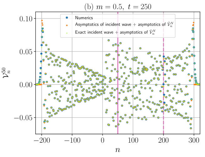
Figure 1: The particle velocity ${\mathcal{V}}_{n}^{N}$ versus the spatial variable $n$. The source position is indicated by the vertical magenta solid line. The right leading scattered wave-front is indicated by the vertical magenta dashed line. (a) The case of a heavy defect, (b) the case of a light defect

Remark 5.6.

Of course, from a pure formal point of view, the localized mode contribution defined by Eq. (5.42) is the principal part of the solution near the defect. For very large times, when the propagating component of the wave-field totally vanishes, the solution near the defect equals the right-hand side of Eq. (5.42). However, in this paper, we are mostly interested in the previous stages of the wave process, when the propagating component still dominates over the localized one.

6 Heat transport: the slow and fast thermal motions

In what follows, we consider the kinetic energy (heat) transport problem formulated in Sect. 3.2.

6.1 $n\leq 0$

Now we calculate the thermal fundamental solution (3.19) taking ${\mathcal{V}}_{n}^{N}=({\mathcal{V}}_{n}^{N})^{\mathrm{pass}}$ and separate the slow and the fast motions following Shishkina and Gavrilov (2023); Gavrilov (2022). Consider the case $n<0$. Due to Eqs. (3.19), (5.30)

$$\mathcal{T}_{n}^{N}=\frac{2m_{n}H(1-w)w^{2}\cos^{2}\big{(}\omega t+\psi+\frac{\pi}{4}\big{)}}{\pi t\sqrt{1-w^{2}}(w^{2}+(m-1)^{2}(1-w^{2}))}+o(t^{-1})=\bar{\mathcal{T}}_{n}^{N}+\hat{\mathcal{T}}_{n}^{N}+o(t^{-1}),\quad w\not\simeq 1;$$ (6.1)

where

$$\bar{\mathcal{T}}_{n}^{N}=\frac{m_{n}H(1-w)w^{2}}{\pi t\sqrt{1-w^{2}}\left((m-1)^{2}\left(1-w^{2}\right)+w^{2}\right)}\\ =\frac{m_{n}H_{-}(n-N)^{2}}{\pi\sqrt{t^{2}-(n-N)^{2}}\big{(}(n-N)^{2}+(m-1)^{2}(t^{2}-(n-N)^{2})\big{)}}$$ (6.2)

is the slow motion, and

$$\hat{\mathcal{T}}_{n}^{N}=-\bar{\mathcal{T}}_{n}^{N}\sin 2(\omega_{-}t+\psi_{-})$$ (6.3)

is the fast motion.

6.2 $n>0$

To calculate the thermal fundamental solution $\mathcal{T}_{n}^{N}$ for $n>0$, we use approximate solution (5.32):

$$\mathcal{T}_{n}^{N}\simeq\frac{2m_{n}H_{+}(m-1)^{2}\sqrt{t^{2}-(n+N)^{2}}\sin^{2}\big{(}\omega_{+}t+\psi_{+}+\frac{\pi}{4}\big{)}}{\pi((n+N)^{2}+(m-1)^{2}(t^{2}-(n+N)^{2}))}+\frac{2m_{n}H_{-}\cos^{2}\big{(}\omega_{-}t+\frac{\pi}{4}\big{)}}{\pi\sqrt{t^{2}-(n-N)^{2}}}\\ -\frac{4m_{n}H_{+}(m-1)\sqrt[4]{t^{2}-(n+N)^{2}}\sin\big{(}\omega_{+}t+\psi_{+}+\frac{\pi}{4}\big{)}\cos\big{(}\omega_{-}t+\frac{\pi}{4}\big{)}}{\pi\sqrt[4]{t^{2}-(n-N)^{2}}\sqrt{(n+N)^{2}+(m-1)^{2}(t^{2}-(n+N)^{2})}}.$$ (6.4)

The last equation can be transformed into the following form:

$$\mathcal{T}_{n}^{N}\simeq\bar{\mathcal{T}}_{n}^{N}+\hat{\mathcal{T}}_{n}^{N},$$ (6.5)

where

$$\bar{\mathcal{T}}_{n}^{N}=m_{n}\bar{T}_{n-N}+\breve{\mathcal{T}}_{n}^{N}$$ (6.6)

is the slow motion,

$$\breve{\mathcal{T}}_{n}^{N}\stackrel{{\scriptstyle\mbox{\scriptsize def}}}{{=}}\frac{H_{+}m_{n}(m-1)^{2}\sqrt{t^{2}-(n+N)^{2}}}{\pi\big{(}(n+N)^{2}+(m-1)^{2}(t^{2}-(n+N)^{2})\big{)}}$$ (6.7)

is the scattered component of the slow motion;

$$\hat{\mathcal{T}}_{n}^{N}=m_{n}\hat{T}_{n-N}+\breve{\mathcal{T}}_{n}^{N}\sin 2(\omega_{+}t+\psi_{+})\\ -\frac{2m_{n}H_{+}(m-1)\sqrt[4]{t^{2}-(n+N)^{2}}{\Big{(}\cos\big{(}(\omega_{+}+\omega_{-})t+\psi_{+}\big{)}+\sin\big{(}(\omega_{+}-\omega_{-})t+\psi_{+}\big{)}\Big{)}}}{\pi\sqrt[4]{t^{2}-(n-N)^{2}}\sqrt{(n+N)^{2}+(m-1)^{2}(t^{2}-(n+N)^{2})}}$$ (6.8)

is the fast motion; $\bar{T}_{n-N}$ and $\hat{T}_{n-N}$ are the slow and fast motions in a uniform chain, defined by Eqs. (6.10) and (6.11), respectively.

Remark 6.1.

The thermal fundamental solution $T_{n-N}$ in a uniform chain, which is defined by (3.21), can be decoupled in the same way into the following superposition Shishkina and Gavrilov (2023); Gavrilov (2022):

$$T_{n-N}=\bar{T}_{n-N}+\hat{T}_{n-N},$$ (6.9)

where

$$\bar{T}_{n-N}\stackrel{{\scriptstyle\mbox{\scriptsize def}}}{{=}}\frac{H_{-}}{\pi\sqrt{1-w^{2}}}=\frac{H_{-}}{\pi\sqrt{t^{2}-(n-N)^{2}}},$$ (6.10)

$$\hat{T}_{n-N}\stackrel{{\scriptstyle\mbox{\scriptsize def}}}{{=}}-\bar{T}_{n-N}\sin 2\omega_{-}t$$ (6.11)

are the slow and fast motions in the uniform chain, respectively.

Remark 6.2.

Since ${\mathcal{V}}_{n}^{N}$ is a continuum quantity (see Remark 5.3), the slow $\bar{\mathcal{T}}_{n}^{N}$ and the fast $\hat{\mathcal{T}}_{n}^{N}$ motions can be naturally continualized in the range $|n|\geq 1$, where $m_{n}=1$, see Remark 12 in Shishkina and Gavrilov (2023).

Thus, the slow motion is the thermal fundamental solution averaged over the fast phases, namely, over

$$\varphi_{0}\stackrel{{\scriptstyle\mbox{\scriptsize def}}}{{=}}2(\omega_{-}t+\psi_{-})$$ (6.12)

for $n\leq 0$;

$$\varphi_{1}\stackrel{{\scriptstyle\mbox{\scriptsize def}}}{{=}}2(\omega_{+}t+\psi_{+}),\quad\varphi_{2}\stackrel{{\scriptstyle\mbox{\scriptsize def}}}{{=}}2\omega_{-}t,\quad\varphi_{3}\stackrel{{\scriptstyle\mbox{\scriptsize def}}}{{=}}(\omega_{+}+\omega_{-})t+\psi_{+},\quad\varphi_{4}\stackrel{{\scriptstyle\mbox{\scriptsize def}}}{{=}}(\omega_{+}-\omega_{-})t+\psi_{+}$$ (6.13)

for $n>0$.

Figure 2: Frequencies $\omega_{-}$ and $\omega_{+}$ versus $n$. The source position is indicated by the vertical magenta solid line. The right leading reflected wave front is indicated by the vertical magenta dashed line

Remark 6.3.

In Fig. 2 one can see the plots of frequencies $\omega_{-}$ and $\omega_{+}$ versus $n$. One can observe that at the leading wave-fronts (5.34) one of the fast phases $\varphi_{0}$ or $\varphi_{2}$ transforms to a slow quantity (for $n<0$ and $n>0$, respectively). In principle, this breaks the slow-and-fast decoupling, but it is not a big problem for us since asymptotics (5.7) is in any case wrong at these wave-fronts (see Remark 5.35). For $n>0$, at the leading reflected wave-front (5.35), the phase $\varphi_{1}$ transforms to a slow quantity. This also corresponds to a domain where approximation (5.31) is not valid (see Remark 5.35). Additionally, the phase $\varphi_{4}$ transforms to a slow quantity for $n\to+0,\ n\in\mathbb{R}$. This breaks at $n\to+0$ the slow-and-fast decoupling for $\mathcal{T}_{n}^{N}$, which is proportional to $({\mathcal{V}}_{n}^{N})^{2}$: the fast motions caused by the incident and reflected waves originate a slow motion. The last observation will be illustrated in what follows; see Sect. 6.3.

6.3 Comparison with numerics

In Fig. 3, we present a spatial plot of the fundamental solution for the kinetic temperature $\mathcal{T}_{n}^{N}$ expressed by Eq. (3.19) and obtained by two approaches. In the framework of the first approach, particle velocities ${\mathcal{V}}_{n}^{N}(t)$ in Eq. (3.19) are found numerically solving system of ordinary differential equations (3.1) with periodic boundary conditions Gavrilov et al. (2019). In the second case, we use the obtained above analytic approximations for the fundamental solution ${\mathcal{V}}_{n}^{N}(t)$, which lead to Eqs. (6.1)–(6.3) (for $n\leq 0$) or Eqs. (6.5)–(6.11) (for $n>0$). Here, $n\in\mathbb{Z}$ or $n\in\mathbb{R}$ for the discrete approximation or for the continuum one, respectively. One can see that discrete approximation is in excellent agreement with numerics everywhere except near leading wave-fronts (5.34), where asymptotics (5.7) is not valid (see Remark 5.35). The agreement is a bit worse near the reflected wave leading front (5.35) (see Remark 5.35 again).

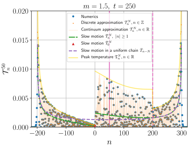
Figure 3: Kinetic temperature $\mathcal{T}_{n}^{N}$ versus spatial variable $n$. The source position is indicated by the vertical magenta solid line. The right leading reflected wave-front is indicated by the vertical magenta dashed line

The slow motion $\bar{\mathcal{T}}_{n}^{N}$, which is also plotted in Fig. 3, has essentially different limiting values at the boundaries for domains of continuity $n=\pm 1$, $n\in\mathbb{R}$. It is minimal (and close to zero) for small non-positive $n$, where a thermal shadow behind the defect is forming. For small positive values of $n$, the slow motion is essentially larger. Thus, at the defect, one can observe a pronounced jump discontinuity of the slow kinetic temperature.

One can see that the slow motion looks like a spatial average for $\mathcal{T}_{n}^{N}$. In the ranges where the fast motion contains a unique harmonic, we can introduce “a peak temperature”

$$\mathfrak{T}_{n}^{N}\stackrel{{\scriptstyle\mbox{\scriptsize def}}}{{=}}2\bar{\mathcal{T}}_{n}^{N},\quad n\in\mathbb{R};\quad n\leq 0\quad\text{or}\quad n>t-N.$$ (6.14)

One can see that the plot for $\mathfrak{T}_{n}^{N}$ looks like the envelope for $\bar{\mathcal{T}}_{n}^{N},\ n\in\mathbb{R}$ in these intervals. In the range $0<n<t-N$, where the fast motion consists of multiple harmonics, see Eq. (6.8), a beat is observed since one of a number of the fast phases becomes a slow quantity for $n\to+0,\ n\in\mathbb{R}$; see Remark 6.3. Introducing the peak temperature as

$$\mathfrak{T}_{n}^{N}\stackrel{{\scriptstyle\mbox{\scriptsize def}}}{{=}}4\bar{\mathcal{T}}_{n}^{N},\quad n\in\mathbb{R};\quad 0<n<t-N,$$ (6.15)

one can see that for small enough positive $n$, the plot for $\mathfrak{T}_{n}^{N}$ again looks like the envelope for $\bar{\mathcal{T}}_{n}^{N}$, $n\in\mathbb{R}$. Thus, the value of the slow temperature for small $n>0$ is close to a quarter of the “nearest global maximum value” for $\mathcal{T}_{n}^{N}$, $n\in\mathbb{R}$, which is observed in Fig. 3 at $n\approx 15.6$.

In Fig. 4, we present temporal plots of the fundamental solution for the kinetic temperature $\mathcal{T}_{n}^{N}$ obtained for several values of $n>0$ by the same two approaches (numeric and analytic ones) as we used for Fig. 3. Again, in the range $N-n<t<N+n$, where the fast motion contains a unique harmonic, the plot for $\mathfrak{T}_{n}^{N}$ is the envelope for $\mathcal{T}_{n}^{N}$. For larger times $t>N+n$ the peak temperature $\mathfrak{T}_{n}^{N}$ again becomes the envelope for $\mathcal{T}_{n}^{N}$ after some transient process. The beat period becomes infinity for $n\to+0$; therefore, the approximate description of the energy transport by the slow motion becomes a bit doubtful for small positive $n$ (see Fig. 4(a)). For larger $n$, this quantity again acquires a clear physical meaning (see Fig. 4(b)–(c)), though the beat period grows and approaches infinity as $t\to\infty$.

In Fig. 5, we present the temporal plot of the fundamental solution $\mathcal{T}_{n}^{N}$ obtained for $n=0$. One can see that the fast motion contains a unique harmonic, and the plot for $\mathfrak{T}_{n}^{N}$ is the envelope for $\mathcal{T}_{n}^{N}$ as expected. The plots for various $n<0$ have the same qualitative character as for $n=0$, and, thus, we do not demonstrate more ones.

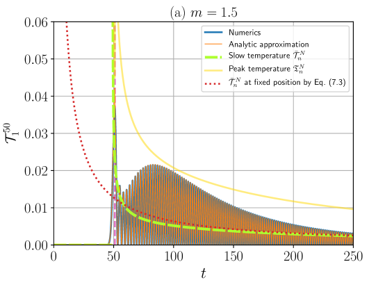
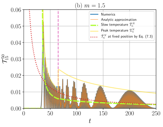
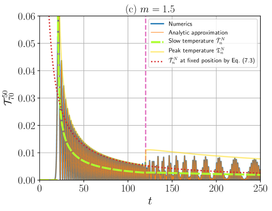
Figure 4: Kinetic temperature $\mathcal{T}_{n}^{N}$ versus time $t$ for various positive $n$. The instant of coming of the leading reflected wave-front is indicated by the vertical magenta dashed line

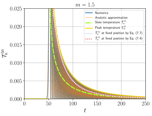
Figure 5: Kinetic temperature $\mathcal{T}_{n}^{N}$ versus time $t$ ($n=0$)

7 Anti-localization for $n\leq 0$: a thermal shadow behind the defect, the Kapitza thermal resistance

In Sect. 6.3, we have shown numerically that the slow temperature $\bar{\mathcal{T}}_{n}^{N}$ quickly changes near the defect. Thus, we observe the non-stationary analogue of the effect characterized by the Kapitza thermal resistance Kapitza (1941). Note that in Paul and Gendelman (2020); Gendelman and Paul (2021) a similar model is used to describe the Kapitza thermal resistance in the case where two stationary thermal sources are located at the ends of a finite chain with an isotopic defect.

Let us formally calculate for a fixed $n>0$ and $n\leq 0$ the large time asymptotics of the components $m_{n}\bar{T}_{n-N}$ and $\breve{\mathcal{T}}^{N}_{n}$ in the right-hand side of Eq. (6.6) of the slow temperature $\bar{\mathcal{T}}^{N}_{n}$.

For $n>0,\ n\in\mathbb{Z}$ (or $n\geq 1,\ n\in\mathbb{R}$ if we discuss continuum quantities), according to (3.21), (6.7), we have: $m_{n}=1$,

$$m_{n}\bar{T}_{n-N}=\frac{1}{\pi t}+O(t^{-3}),$$ (7.1)

$$\breve{\mathcal{T}}_{n}^{N}=\frac{1}{\pi t}+O(t^{-3}),$$ (7.2)

and, thus,

$$\bar{\mathcal{T}}_{n}^{N}=\frac{2}{\pi t}+O(t^{-3}).$$ (7.3)

Formulae (7.1)–(7.3) are clearly derived in a not entirely correct way, i.e., by calculating the asymptotics at a fixed position of the solution obtained at a moving point of observation. They demonstrate that reflection from the defect results in the doubling of the slow temperature $\bar{\mathcal{T}}_{n}^{N}$ for all $n>0$. In Fig. 4, one can see that numerical calculations confirm such a conclusion for very large times: the red dotted curves asymptotically approach the corresponding green dashed ones in all plots. According to Eqs. (7.1)–(7.3), the slow temperature at this final stage does not depend on $n$ for $n>0$.

For $n\leq 0$, according to Eq. (6.2), one obtains:

$$\bar{\mathcal{T}}_{n}^{N}=\frac{m_{n}(n-N)^{2}}{\pi(m-1)^{2}t^{3}}+O(t^{-4}).$$ (7.4)

Remark 7.1.

The result for $n\leq 0$, generally speaking, is obtained incorrectly since we have dropped the terms of order $o(t^{-1/2})$ when calculating the asymptotics (5.30) of the particle velocity $({\mathcal{V}}_{n}^{N})^{\mathrm{pass}}$ at a moving point of observation. These terms correspond to the terms of order $o(t^{-1})$ in expansions for $\mathcal{T}_{n}^{N}$, whereas the principal term in (7.4) is of order $t^{-3}$. However, one can see in Fig. 5 that formula (7.4) describes the final stage of evolution for $\mathcal{T}_{n}^{N}$ quite well. To verify Eq. (7.4), in Sect. 7.1, we construct the large time asymptotics for the particle velocity ${\mathcal{V}}_{n}^{N}$ and the slow temperature $\bar{\mathcal{T}}_{n}^{N}$ at a fixed position $n\leq 0$.

7.1 Asymptotics for the particle velocity and the slow temperature at a fixed position $n\leq 0$

To calculate the fixed position asymptotics, we deal with integral representation (5.1) and apply the method of stationary phase. The only critical point is the cut-off frequency; thus, we need to calculate the corresponding contribution for integrals over the pass-band and the stop-band. Take $n\leq 0$. We base on the expansions for the amplitude

$$C_{n}^{N}\stackrel{{\scriptstyle\mbox{\scriptsize def}}}{{=}}\Omega\mathcal{G}_{n}^{N}$$ (7.5)

in the pass-band and the stop-band, see Eqs. (B.9), (C.8) which are obtained in Appendices B and C, respectively. Now, the total contribution from the cut-off frequency can be calculated in the same way as in Sect. 7.3 of Shishkina and Gavrilov (2023), where the corresponding expansions of the amplitude are given by Eqs. (7.13) and (7.49), respectively. The first (zero order) terms in the right-hand sides of Eqs. (B.9), (C.8) are equal to each other, and the corresponding total contribution from the pass-band and the stop-band is zero. The second (square root) terms equal the corresponding terms in the right-hand side of Eqs. (7.13), (7.49) in Shishkina and Gavrilov (2023) with accuracy to the multiplier $(-1)^{N-n}\big{(}1+2(N-n)(m-1)\big{)}$. Thus, one gets (see Eqs. (7.54) and (10.6) in Shishkina and Gavrilov (2023), respectively):

$${\mathcal{V}}_{n}^{N}=\frac{(-1)^{N-n}\big{(}1+2({N-n})(m-1)\big{)}\sin\big{(}2t-\frac{\pi}{4}\big{)}}{2\sqrt{\pi}(m-1)^{2}t^{3/2}}+o(t^{-3/2}),$$ (7.6)

$$\bar{\mathcal{T}}_{n}^{N}=\frac{m_{n}\big{(}1+2({N-n})(m-1)\big{)}^{2}}{4\pi(m-1)^{4}t^{3}}+o(t^{-3}).$$ (7.7)

Provided that

$$2(N-n)|m-1|\gg 1,$$ (7.8)

i.e., number $N$ is large enough, the right-hand sides of Eqs. (7.4) and (7.7) almost coincide (see Fig. 5). Thus, Eq. (7.4) really provides “an almost correct result”.

7.2 The non-stationary transmission function for the kinetic temperature

The obtained Eqs. (7.6), (7.7) show that for all $n\leq 0$, we observe the phenomenon of anti-localization of non-stationary quasi-waves. This is the zeroing of the non-localized propagating component of the wave-field in a neighbourhood of an inclusion Shishkina and Gavrilov (2023); Shishkina et al. (2023). This neighbourhood expands with time, capturing more and more material points of the chain. However, this process never leads to a total blocking Glushkov et al. (2006b, a) of energy propagation toward $n\to-\infty$ but only to some distortion of the incident wave-field. Indeed, in the interval $n\leq 0$, consider the ratio

$$\mathcal{R}(w)=\frac{\bar{\mathcal{T}}_{n}^{N}}{\bar{T}_{n-N}}=\frac{w^{2}}{(m-1)^{2}\left(1-w^{2}\right)+w^{2}}$$ (7.9)

as the function of the speed $w$ defined by Eq. (5.14), which we call the non-stationary transmission function for the kinetic temperature. Here ${\bar{\mathcal{T}}_{n}^{N}}$ and $\bar{T}_{n-N}$ are calculated by Eqs. (6.2) and (6.10), respectively. The plot of ratio $\mathcal{R}$ versus $w$ is presented in Fig. 6.

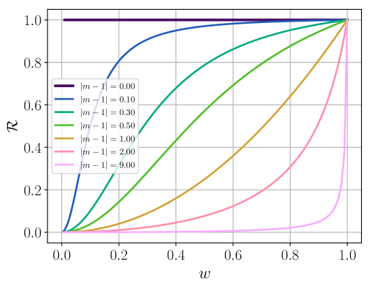
Figure 6: The non-stationary transmission function for the kinetic temperature $\mathcal{R}$ versus $w$

One can see that the greater the quantity $|m-1|$, the wider the anti-localization zone (i.e., the thermal shadow) behind the defect, and more wave energy concentrates closer to the leading wave-front $w=1$. For $m\neq 1$, any material particle of the chain with $n\leq 0$ after some time from the instant of passing the leading wave-front moving at $w=1$ enters the thermal shadow, where the kinetic temperature decreases according to Eq. (7.7) as $O(t^{-3})$.

Remark 7.2.

The cold point at the defect (see Fig. 8(a) in Gendelman and Paul (2021)), apparently, is the only anti-localization point observed in the system with two thermal sources at both sides of an isotopic defect.

Remark 7.3.

The anti-localization of non-stationary waves was introduced previously in the framework of the problems Gavrilov et al. (2023); Shishkina and Gavrilov (2023); Shishkina et al. (2023), where a loading is applied to a defect. In this paper, we show for the first time how the anti-localization influences a wave process when a loading and a defect are located at different positions.

8 Conclusion

In the paper, we have considered two problems. The first one is the deterministic problem concerning elastic wave scattering on an isotopic defect in a one-dimensional harmonic crystal (a linear chain). The chain is subjected to a unit impulse point loading applied to a particle far enough from the defect. In the framework of the second problem, we assume that applied point impulse excitation has random amplitude. This allows one to model the heat transport in the chain and across the defect as the transport of the mathematical expectation for the kinetic energy and to use the conception of the kinetic temperature.

The most important result related to the first (scattering) problem is Eqs. (5.28), (5.31), which provide for $t\to\infty$ a continuum approximation for the fundamental solution describing the scattered wave-field in the time domain. This approximation is obtained as a large time asymptotics at a moving point of observation, and it is in excellent agreement with corresponding numerical calculations (see Fig. 1). We have shown that in the case of loading applied far enough from the defect, which is assumed in the paper, the scattered wave-fields caused by heavy ($m>1$) and light ($m<1$) defects are qualitatively similar. The localized non-vanishing in time oscillation, which exists in the system in the case $m<1$ Montroll and Potts (1955); Shishkina and Gavrilov (2023), has exponentially vanishing with the distance (between the defect and the point of the loading) amplitude; see Eq. (5.42). Thus, the localized oscillation can be neglected. This is an essential difference from the case when the loading is applied at the defect considered in our previous paper Shishkina and Gavrilov (2023). In the latter case, the wave-field caused by a light defect contains a pronounced non-vanishing localized component.

It is interesting that the choice of the moving point of observation, which we use to get the corresponding asymptotics is generally ambiguous. In previous studies Shishkina and Gavrilov (2023); Shishkina et al. (2023); Gavrilov et al. (2023), we considered the case when the loading was applied to the defect. We followed the natural choice, which was to consider the fronts emerging at the instance of the impulse loading and then moving at a constant speed away from the loaded particle, i.e., from the defect. Now, we consider the problem, where the loading and the defect are in the different positions, and it is not clear what is “a natural choice”. We have tried to use various choices (see Appendix A) and obtained different formally correct asymptotics. We have shown that the only one among the proposed asymptotics is applicable as an approximate solution, which characterizes the wave-field in terms of the particle number $n$ co-ordinate and time $t$.

The most important result related to the second (heat transport) problem is Eqs. (6.2), (6.7), which provide for $t\to\infty$ the expressions for the slow (in time) component of the kinetic temperature in the chain, i.e., the slow motion. To intuitively understand what the slow motion is, the reader can look through Figs. 3–5. In discrete harmonic systems, where a stochastic loading is distributed in space Krivtsov (2015, 2019); Sokolov et al. (2021); Kuzkin and Krivtsov (2017); Kuzkin (2019) or in time Gavrilov et al. (2019); Gavrilov and Krivtsov (2022, 2020), according to numerical calculations, the fast component vanishes. Thus, we expect that to describe the heat transport for such a loading, it is enough to calculate a convolution of the distributed loading with the fundamental solution for the slow motion without any spatial or temporal averaging. However, in the range $n>0$, especially for small $n$, such a description is perhaps too oversimplified; see Remark 6.3 and Sect. 6.3.

The obtained solution allows us to show that there is a thermal shadow behind the defect: the order of vanishing for the slow temperature is larger for the particles behind the defect than for the particles between the loading and the defect (see Eqs. (7.3), (7.4) and Fig. 3). From a pure mathematical point of view, such a result cannot be obtained correctly based on the asymptotic solution at a moving point of observation (see Remark 7.1). Therefore, we have verified and confirmed it by considering asymptotics at a fixed position (see Sect. 7.1). The asymptotics at a fixed position describes only the last stage of the evolution of corresponding quantities, i.e., the particle velocity or the kinetic temperature, whereas the asymptotics at a moving point of observation, suggested in Sect. 5.1.1, describes earlier stages (see Figs. 4, 5). Due to the presence of the shadow, the continuum slow kinetic temperature has a jump discontinuity at the defect. Thus, the system under consideration can be a simple model for the non-stationary phenomenon analogous to one characterized by the Kapitza thermal resistance Gendelman and Paul (2021); Kapitza (1941); Lumpkin et al. (1978); Paul and Gendelman (2020).

The presence of the thermal shadow is related to a non-stationary wave phenomenon, which we call the anti-localization of non-stationary waves. This is the zeroing of the non-localized propagating component of the wave-field in a neighbourhood of an inclusion Shishkina and Gavrilov (2023); Shishkina et al. (2023). In previous studies Shishkina and Gavrilov (2023); Shishkina et al. (2023), where the anti-localization was introduced, the case when the loading and the defect were at the same position was considered (see Remark 7.3). In the latter case, the zeroing is observed in a two-sided neighbourhood of the defect. In this paper, the anti-localization is observed only for the defect and particles behind the defect with respect to the point of loading ($n\leq 0$). This one-sided neighbourhood expands with time, capturing more and more material points of the chain. However, this process never leads to a total blocking of energy propagation toward $n\to-\infty$ (as it is observed, e.g., in Glushkov et al. (2006b, a)), but only to a distortion of the incident wave-field due to the defect. We propose as a measure for this distortion the non-stationary transmission function for the kinetic temperature, which can be calculated by Eq. (7.9). One can see in Fig. 6 that the greater the quantity $|m-1|$ (the absolute value of the difference between the defect mass and the mass of the regular particle), the more distortion of the wave-field is observed at a far zone behind the defect.

We suppose that, without essential modifications, the methodology proposed in this paper can be applied to other similar problems concerning more complicated one-dimensional harmonic crystals and other types of defects (or interfaces).

Funding

This work is supported by the Russian Science Foundation (project 22-11-00338).

Appendix A Asymptotics at alternative moving points of observation

The choice of the moving observation fronts is generally ambiguous. One can try to construct asymptotics on moving observation points different from Eq. (5.14). Consider the case $n\leq 0$ (the scattered wave for $n>0$ as in Sect 5.1.2 can be calculated using the evenness of $(\breve{{\mathcal{V}}}_{n}^{N})^{\mathrm{pass}}$ with respect to $n$). Let us estimate the integral $(\mathcal{I}_{n}^{N})^{\mathrm{pass}}$ on a moving point of observation different from the one given by Eq. (5.14). We can try to use the following moving point of observation instead of Eq. (5.14):

$$|n|=wt.$$ (A.1)

The integral $(\mathcal{I}_{n}^{N})^{\mathrm{pass}}$ (5.13) can be represented in the form of Eq. (5.15), where

$$A^{\mathrm{pass}}(\Omega)=\frac{(m-1)\Omega\mathrm{e}^{\mathrm{i}N\arccos\frac{2-\Omega^{2}}{2}}}{-(4-\Omega^{2})+\mathrm{i}(m-1)\Omega\sqrt{4-\Omega^{2}}},$$ (A.2)

$\phi(\Omega)$ is given by Eq. (5.17). Applying the procedure of the method of stationary phase in the same way as it is done in Sect. 5.1.1, instead of Eq. (5.25) one gets:

$$(\breve{\mathcal{V}}_{n}^{N})^{\mathrm{pass}}=-\frac{H(1-w)(m-1)\sqrt[4]{1-w^{2}}}{\sqrt{\pi t}\big{(}w^{2}+(m-1)^{2}(1-w^{2})\big{)}}\Big{(}\Big{(}(m-1)\sqrt{1-w^{2}}\cos F+w\sin F\Big{)}\cos\Big{(}\omega t+\frac{\pi}{4}\Big{)}\\ +\Big{(}w\cos F-(m-1)\sqrt{1-w^{2}}\sin F\Big{)}\sin\Big{(}\omega t+\frac{\pi}{4}\Big{)}\Big{)}+O(t^{-1}).$$ (A.3)

Here

$$F=F_{0}\arccos(2w^{2}-1),$$ (A.4)

$$F_{0}=N.$$ (A.5)

Formula (A.3) can be transformed into the form of Eq. (5.26), wherein we should substitute

$$\psi_{\ast}=\arctan\frac{w\sin F+(m-1)\sqrt{1-w^{2}}\cos F}{w\cos F-(m-1)\sqrt{1-w^{2}}\sin F}=F+\psi$$ (A.6)

instead of $\psi$ defined by (5.27).

Consider now the following moving point of observation:

$$|n|=w(t-N).$$ (A.7)

In the latter case

$$A^{\mathrm{pass}}(\Omega)=\frac{(m-1)\Omega\mathrm{e}^{\mathrm{i}N(1-w)\arccos\frac{2-\Omega^{2}}{2}}}{-(4-\Omega^{2})+\mathrm{i}(m-1)\Omega\sqrt{4-\Omega^{2}}},$$ (A.8)

and asymptotics for $(\breve{\mathcal{V}}_{n}^{N})^{\mathrm{pass}}$ has the form (A.3), wherein

$$F_{0}=N(1-w).$$ (A.9)

Remark A.1.

Asymptotics (5.25) can be formally obtained by substituting

$$F_{0}=0$$ (A.10)

into Eqs. (A.3), (A.4).

All asymptotics in the form of Eq. (A.3) with various $F_{0}$ defined by (A.5), (A.9), (A.10) are formally correct. According to Eqs. (A.4), (A.6), for various $F_{0}$ the right-hand side of Eq. (A.3) has the same amplitude but different phases. Moreover, formulae (A.1), (A.7), or (5.14) that we use to return to the variables $n$ and $t$ from $w$ and $t$ are also different. Therefore, the applicability of the corresponding asymptotics as an approximate solution in terms of $n$ and $t$ can also be different. To check which approach is better, we calculate the absolute error

$$e_{n}^{N}\stackrel{{\scriptstyle\mbox{\scriptsize def}}}{{=}}({\mathcal{V}}_{n}^{N})_{\mathrm{num}}-V_{n-N}-(\breve{\mathcal{V}}_{n}^{N})^{\mathrm{pass}}_{\mathrm{approx}}$$ (A.11)

using various asymptotics (A.3), (A.4) with $F_{0}$ defined by (A.5), (A.9) or (A.10). Here $({\mathcal{V}}_{n}^{N})_{\mathrm{num}}$ are values for the particle velocities found numerically, $V_{n-N}$ is given by exact formula (3.10), $({\mathcal{V}}_{n}^{N})^{\mathrm{pass}}_{\mathrm{approx}}$ are found by Eq. (A.3) wherein $w$ is found in accordance with the corresponding formula from set (A.1), (A.7), (5.14). The plot for the error $e_{n}^{N}$ is presented in Fig. 7. One can see that the choice of $F_{0}$ in the form of Eq. (A.10) gives the best result, whereas asymptotics with $F_{0}$ in the form of (A.5), (A.9) are practically inapplicable as an approximate solution in terms of variables $n$ and $t$.

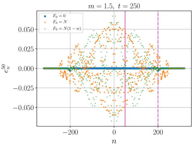
Figure 7: Error $e_{n}^{N}$ versus $n$. The source position is indicated by the vertical magenta solid line. The right leading reflected wave-front is indicated by the vertical magenta dashed line

Appendix B Fixed position asymptotics for $n\leq 0$: the amplitude expansion near the cut-off frequency in the pass-band

Take $n\leq 0$. For $C_{n}^{N}$ defined by Eq. (7.5), one has

$$C_{n}^{N}(\Omega)=\big{(}A(\Omega)+B(\Omega)\big{)}E_{n}^{N}(\Omega),$$ (B.1)

$$A(\Omega)E_{n}^{N}(\Omega)=\Omega\breve{\mathcal{G}}_{n}^{N},\qquad B(\Omega)E_{n}^{N}(\Omega)=\Omega G_{n-N}.$$ (B.2)

In the pass-band, $A(\Omega)$ is defined by Eq. (5.16),

$$B(\Omega)=-\frac{1}{\mathrm{i}\sqrt{4-\Omega^{2}}},$$ (B.3)

$$E_{n}^{N}(\Omega)={\mathrm{e}}^{\mathrm{i}({N-n})\arccos\frac{2-\Omega^{2}}{2}},$$ (B.4)

see Eqs. (4.5), (4.6), (4.8), (5.1)–(5.5), (5.13). For $\Omega\to 2-0$, one can obtain the following asymptotic expansions:

$$A(\Omega)=\frac{-\mathrm{i}}{2\sqrt{2-\Omega}}-\frac{1}{2(m-1)}+\frac{\mathrm{i}(-m^{2}+2m+7)\sqrt{2-\Omega}}{16(m-1)^{2}}+O(2-\Omega),$$ (B.5)

$$B(\Omega)=\frac{\mathrm{i}}{2\sqrt{2-\Omega}}+\frac{\mathrm{i}\sqrt{2-\Omega}}{16}+O\big{(}(2-\Omega)^{3/2}\big{)},$$ (B.6)

$$E_{n}^{N}(\Omega)=(-1)^{N-n}-2\mathrm{i}({N-n})(-1)^{N-n}\sqrt{2-\Omega}+O(2-\Omega).$$ (B.7)

Now, one gets

$$A(\Omega)+B(\Omega)=-\frac{1}{2(m-1)}+\frac{\mathrm{i}\sqrt{2-\Omega}}{2(m-1)^{2}}+O(2-\Omega),$$ (B.8)

$$C_{n}^{N}(\Omega)=-\frac{(-1)^{N-n}}{2(m-1)}+\frac{\mathrm{i}(-1)^{N-n}\big{(}1+2({N-n})(m-1)\big{)}\sqrt{2-\Omega}}{2(m-1)^{2}}+O(2-\Omega).$$ (B.9)

Appendix C Fixed position asymptotics for $n\leq 0$: the amplitude expansion near the cut-off frequency in the stop-band

In the stop-band, we again have Eqs. (B.1), (B.2), wherein

$$A(\Omega)=\frac{\Omega^{3}(m-1)}{\Big{(}-\Omega^{2}+2\mathrm{e}^{-\operatorname{arccosh}\frac{\Omega^{2}-2}{2}}+2\Big{)}\Big{(}-m\Omega^{2}+2\mathrm{e}^{-\operatorname{arccosh}\frac{\Omega^{2}-2}{2}}+2\Big{)}},$$ (C.1)

$$B(\Omega)=\frac{\Omega}{-\Omega^{2}+2\mathrm{e}^{-\operatorname{arccosh}\frac{\Omega^{2}-2}{2}}+2},$$ (C.2)

$$E_{n}^{N}(\Omega)=(-1)^{{N-n}}\mathrm{e}^{-({N-n})\operatorname{arccosh}\frac{\Omega^{2}-2}{2}},$$ (C.3)

see Eqs. (4.5), (4.7), (4.9), (5.1)–(5.5), (5.36). For $\Omega\to 2+0$, one can obtain the following asymptotic expansions:

$$A(\Omega)=\frac{1}{2\sqrt{\Omega-2}}-\frac{1}{2(m-1)}-\frac{\left(m^{2}-2m-7\right)\sqrt{\Omega-2}}{16(m-1)^{2}}+O(\Omega-2),$$ (C.4)

$$B(\Omega)=-\frac{1}{2\sqrt{\Omega-2}}+\frac{\sqrt{\Omega-2}}{16}+O\big{(}(\Omega-2)^{3/2}\big{)},$$ (C.5)

$$E_{n}^{N}(\Omega)=(-1)^{N-n}\big{(}1-2({N-n})\sqrt{\Omega-2}+O(\Omega-2)\big{)}.$$ (C.6)

Now, one gets

$$A(\Omega)+B(\Omega)=-\frac{1}{2(m-1)}+\frac{\sqrt{\Omega-2}}{2(m-1)^{2}}+O(\Omega-2),$$ (C.7)

$$C_{n}^{N}(\Omega)=-\frac{(-1)^{N-n}}{2(m-1)}+\frac{(-1)^{N-n}\big{(}1+2({N-n})(m-1)\big{)}\sqrt{\Omega-2}}{2(m-1)^{2}}+O(\Omega-2).$$ (C.8)

References

- Chen et al. [2012] S. Chen, Q. Wu, C. Mishra, J. Kang, H. Zhang, K. Cho, W. Cai, A. A. Balandin, and R. S. Ruoff. Thermal conductivity of isotopically modified graphene. Nature Materials, 11(3):203–207, 2012.
- Erdélyi [1956] A. Erdélyi. Asymptotic expansions. Dover Publications, New York, 1956.
- Fedoryuk [1977] M. V. Fedoryuk. Metod perevala [The Saddle-Point Method]. Nauka [Science], Moscow, 1977. In Russian.
- Fellay et al. [1997] A. Fellay, F. Gagel, K. Maschke, A. Virlouvet, and A. Khater. Scattering of vibrational waves in perturbed quasi-one-dimensional multichannel waveguides. Physical Review B, 55(3):1707–1717, 1997.
- Gavrilov [2022] S. N. Gavrilov. Discrete and continuum fundamental solutions describing heat conduction in a 1D harmonic crystal: Discrete-to-continuum limit and slow-and-fast motions decoupling. International Journal of Heat and Mass Transfer, 194:123019, 2022.
- Gavrilov and Krivtsov [2019] S. N. Gavrilov and A. M. Krivtsov. Thermal equilibration in a one-dimensional damped harmonic crystal. Physical Review E, 100(2):022117, 2019.
- Gavrilov and Krivtsov [2020] S. N. Gavrilov and A. M. Krivtsov. Steady-state kinetic temperature distribution in a two-dimensional square harmonic scalar lattice lying in a viscous environment and subjected to a point heat source. Continuum Mechanics and Thermodynamics, 32(1):41–61, 2020.
- Gavrilov and Krivtsov [2022] S. N. Gavrilov and A. M. Krivtsov. Steady-state ballistic thermal transport associated with transversal motions in a damped graphene lattice subjected to a point heat source. Continuum Mechanics and Thermodynamics, 34(1):297–319, 2022.
- Gavrilov et al. [2019] S. N. Gavrilov, A. M. Krivtsov, and D. V. Tsvetkov. Heat transfer in a one-dimensional harmonic crystal in a viscous environment subjected to an external heat supply. Continuum Mechanics and Thermodynamics, 31:255–272, 2019.
- Gavrilov et al. [2023] S. N. Gavrilov, E. V. Shishkina, and Yu. A. Mochalova. An example of the anti-localization of non-stationary quasi-waves in a 1D semi-infinite harmonic chain. In Proc. Int. Conf. Days on Diffraction (DD), 2023. IEEE, 2023. Accepted.
- Gendelman and Paul [2021] O. V. Gendelman and J. Paul. Kapitza thermal resistance in linear and nonlinear chain models: Isotopic defect. Physical Review E, 103(5):052113, 2021.
- Glushkov et al. [2006a] E. Glushkov, N. Glushkova, M. Golub, and A. Boström. Natural resonance frequencies, wave blocking, and energy localization in an elastic half-space and waveguide with a crack. The Journal of the Acoustical Society of America, 119(6):3589–3598, 2006a.
- Glushkov et al. [2006b] E. V. Glushkov, N. V. Glushkova, and M. V. Golub. Blocking of traveling waves and energy localization due to the elastodynamic diffraction by a crack. Acoustical Physics, 52(3):259–269, 2006b.
- Hemmer [1959] P. C. Hemmer. Dynamic and Stochastic Types of Motion in the Linear Chain. PhD thesis, Norges tekniske høgskole, Trondheim, 1959.
- Jex [1986] H. Jex. The transmission and reflection of acoustic and optic phonons from a solid-solid interface treated in a linear chain model. Zeitschrift für Physik B, 63(1):91–95, 1986.
- Kakodkar and Feser [2015] R. R. Kakodkar and J. P. Feser. A framework for solving atomistic phonon-structure scattering problems in the frequency domain using perfectly matched layer boundaries. Journal of Applied Physics, 118(9):094301, 2015.
- Kannan [2013] V. Kannan. Heat conduction in low dimensional lattice systems. PhD thesis, Rutgers the State University of New Jersey – New Brunswick, 2013.
- Kapitza [1941] P. L. Kapitza. Heat transfer and superfluidity of helium II. Physical Review, 60(4):354–355, 1941.
- Kashiwamura [1962] S. Kashiwamura. Statistical dynamical behaviors of a one-dimensional lattice with an isotopic impurity. Progress of Theoretical Physics, 27(3):571–588, 1962.
- Kosevich [1997] Yu. A. Kosevich. Capillary phenomena and macroscopic dynamics of complex two-dimensional defects in crystals. Progress in Surface Science, 55(1):1–57, 1997.
- Kosevich [2008] Yu. A. Kosevich. Multichannel propagation and scattering of phonons and photons in low-dimension nanostructures. Physics-Uspekhi, 51(8), 2008.
- Kossevich [1999] A. M. Kossevich. The crystal lattice: phonons, solitons, dislocations. Wiley-VCH, Berlin, 1999. ISBN 3-527-40220-9.
- Koster [1954] G. F. Koster. Theory of scattering in solids. Physical Review, 95(6):1436–1443, 1954.
- Krivtsov [2014] A. M. Krivtsov. Energy oscillations in a one-dimensional crystal. Doklady Physics, 59(9):427–430, 2014.
- Krivtsov [2015] A. M. Krivtsov. Heat transfer in infinite harmonic one-dimensional crystals. Doklady Physics, 60(9):407–411, 2015.
- Krivtsov [2019] A. M. Krivtsov. The ballistic heat equation for a one-dimensional harmonic crystal. In H. Altenbach et al., editors, Dynamical Processes in Generalized Continua and Structures, volume 103 of Advanced Structured Materials, pages 345–358. Springer, 2019.
- Kuzkin [2019] V. A. Kuzkin. Unsteady ballistic heat transport in harmonic crystals with polyatomic unit cell. Continuum Mechanics and Thermodynamics, 31(6):1573–1599, 2019.
- Kuzkin [2023] V. A. Kuzkin. Acoustic transparency of the chain-chain interface. Physical Review E, 107(6):065004, 2023.
- Kuzkin and Krivtsov [2017] V. A. Kuzkin and A. M. Krivtsov. Fast and slow thermal processes in harmonic scalar lattices. Journal of Physics: Condensed Matter, 29(50):505401, 2017.
- Lee et al. [1989] M. H. Lee, J. Florencio, and J. Hong. Dynamic equivalence of a two-dimensional quantum electron gas and a classical harmonic oscillator chain with an impurity mass. Journal of Physics A, 22(8):L331–L335, 1989.
- Liazhkov [2023] S. D. Liazhkov. Unsteady thermal transport in an instantly heated semi-infinite free end Hooke chain. Continuum Mechanics and Thermodynamics, 35(2):413–430, 2023.
- Lifshitz and Kosevich [1966] I. M. Lifshitz and A. M. Kosevich. The dynamics of a crystal lattice with defects. Reports on Progress in Physics, 29(1):217–254, 1966.
- Lifšic [1956] M. Lifšic. Some problems of the dynamic theory of non-ideal crystal lattices. Il Nuovo Cimento, 3(S4):716–734, 1956.
- Lumpkin et al. [1978] M. E. Lumpkin, W. M. Saslow, and W. M. Visscher. One-dimensional Kapitza conductance: Comparison of the phonon mismatch theory with computer experiments. Physical Review B, 17(11):4295–4302, 1978.
- Magalinskii [1959] V. B. Magalinskii. Dynamical model in the theory of the brownian motion. Soviet Physics JETP-USSR, 9(6):1381–1382, 1959.
- Mokole et al. [1990] E. L. Mokole, A. L. Mullikin, and M. B. Sledd. Exact and steady-state solutions to sinusoidally excited, half-infinite chains of harmonic oscillators with one isotopic defect. Journal of Mathematical Physics, 31(8):1902–1913, 1990.
- Montroll and Potts [1955] E. W. Montroll and R. B. Potts. Effect of defects on lattice vibrations. Physical Review, 100(2):525–543, 1955.
- Müller [1962] I. Müller. Durch eine äußere Kraft erzwungene Bewegung der mittleren Masse eineslinearen Systems von durch federn verbundenen Massen [The forced motion of the sentral mass in a linear mass-spring chain of masses under the action of an external force]. Diploma thesis, Technical University Aachen, 1962.
- Müller and Weiss [2012] I. Müller and W. Weiss. Thermodynamics of irreversible processes — past and present. The European Physical Journal H, 37(2):139–236, 2012.
- Paul and Gendelman [2020] J. Paul and O. V. Gendelman. Kapitza resistance in basic chain models with isolated defects. Physics Letters A, 384(10):126220, 2020.
- Plyukhin [2020] A. V. Plyukhin. Non-Clausius heat transfer: the example of harmonic chain with an impurity. Journal of Statistical Mechanics: Theory and Experiment, 2020(6):063212, 2020.
- Polanco et al. [2013] C. A. Polanco, C. B. Saltonstall, P. M. Norris, P. E. Hopkins, and A. W. Ghosh. Impedance matching of atomic thermal interfaces using primitive block decomposition. Nanoscale and Microscale Thermophysical Engineering, 17(3):263–279, 2013.
- Rubin [1960] R. J. Rubin. Statistical dynamics of simple cubic lattices. Model for the study of brownian motion. Journal of Mathematical Physics, 1(4):309–318, 1960.
- Rubin [1961] R. J. Rubin. Statistical dynamics of simple cubic lattices. Model for the study of brownian motion. II. Journal of Mathematical Physics, 2(3):373–386, 1961.
- Rubin [1963] R. J. Rubin. Momentum autocorrelation functions and energy transport in harmonic crystals containing isotopic defects. Physical Review, 131(3):964–989, 1963.
- Saito et al. [2018] R. Saito, M. Mizuno, and M. S. Dresselhaus. Ballistic and diffusive thermal conductivity of graphene. Physical Review Applied, 9(2):024017, 2018.
- Saltonstall et al. [2013] C. B. Saltonstall, C. A. Polanco, J. C. Duda, A. W. Ghosh, P. M. Norris, and P. E. Hopkins. Effect of interface adhesion and impurity mass on phonon transport at atomic junctions. Journal of Applied Physics, 113(1):013516, 2013.
- Schrödinger [1914] E. Schrödinger. Zur Dynamik elastisch gekoppelter Punktsysteme. Annalen der Physik, 349(14):916–934, 1914.
- Shishkina and Gavrilov [2023] E. V. Shishkina and S. N. Gavrilov. Unsteady ballistic heat transport in a 1D harmonic crystal due to a source on an isotopic defect. Continuum Mechanics and Thermodynamics, 35:431–456, 2023.
- Shishkina et al. [2023] E. V. Shishkina, S. N. Gavrilov, and Yu. A. Mochalova. The anti-localization of non-stationary linear waves and its relation to the localization. The simplest illustrative problem. Journal of Sound and Vibration, 553:117673, 2023.
- Sokolov et al. [2021] A. A. Sokolov, W. H. Müller, A. V. Porubov, and S. N. Gavrilov. Heat conduction in 1D harmonic crystal: Discrete and continuum approaches. International Journal of Heat and Mass Transfer, 176:121442, 2021.
- Steinbrüchel [1976] Ch. Steinbrüchel. The scattering of phonons of arbitrary wavelength at a solid-solid interface: Model calculation and applications. Zeitschrift für Physik B, 24(3):293–299, 1976.
- Takizawa and Kobayasi [1968a] E. I. Takizawa and K. Kobayasi. Localized vibrations in a system of coupled harmonic oscillators. Chinese Journal of Physics, 5(1):11–17, 1968a.
- Takizawa and Kobayasi [1968b] E. I. Takizawa and K. Kobayasi. On the stochastic types of motion in a system of linear harmonic oscillators. Chinese Journal of Physics, 6(1):39–66, 1968b.
- Temme [2014] N. M. Temme. Asymptotic Methods for Integrals. World Scientific, Singapore, 2014. ISBN 978-9814612159.
- Teramoto and Takeno [1960] E. Teramoto and S. Takeno. Time dependent problems of the localized lattice vibration. Progress of Theoretical Physics, 24(6):1349–1368, 1960.
- Turner [1960] R. E. Turner. Motion of a heavy particle in a one dimensional chain. Physica, 26(4):269–273, 1960.
- Vladimirov [1971] V. S. Vladimirov. Equations of Mathematical Physics. Marcel Dekker, New York, 1971.
- Yu [2019] M. B. Yu. A monatomic chain with an impurity in mass and Hooke constant. The European Physical Journal B, 92:272, 2019.