Information Content based Exploration

Abstract

Sparse reward environments are known to be challenging for reinforcement learning agents. In such environments, efficient and scalable exploration is crucial. Exploration is a means by which an agent gains information about the environment; we expand on this topic and propose a new intrinsic reward that systemically quantifies exploratory behaviour and promotes state coverage by maximizing the information content of a trajectory taken by an agent. We compare our method to alternative exploration-based intrinsic reward techniques, namely Curiosity Driven Learning (CDL) and Random Network Distillation (RND). We show that our information-theoretic reward induces efficient exploration and outperforms in various games, including Montezuma’s Revenge – a known difficult task for reinforcement learning. Finally, we propose an extension that maximizes information content in a discretely compressed latent space which boosts sample-efficiency and generalizes to continuous state spaces.

1 Introduction

Given an agent without knowledge of the environment dynamics, a fundamental question is: what should the agent learn first? When the task is also unknown, the question becomes increasingly complex (Moerland et al., 2020)(Riedmiller et al., 2018). In reward-dense environments, the agent receives a continuous gradient signal that guides learning through interaction (Mnih et al., 2013)(Achiam & Sastry, 2017)(Hong et al., 2018)(Haarnoja et al., 2018). However, for many problems of interest, the most faithful reward specification is sparse, degrading the sample efficiency with which online algorithms can learn desirable policies (Tim Salimans, 2018)(Vecerik et al., 2017)(Singh et al., 2019)(Sekar et al., 2020).

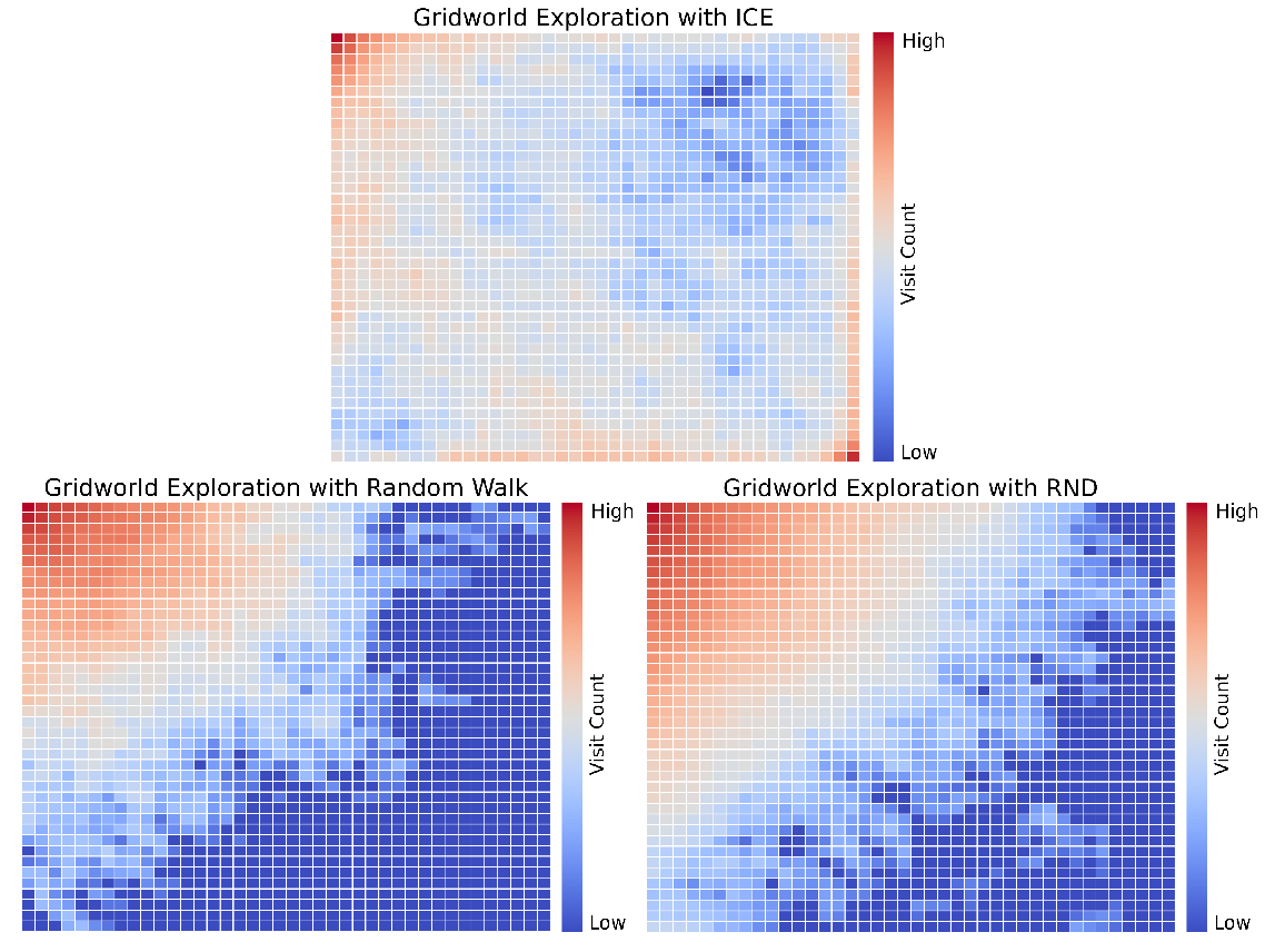
Figure 1: ICE (top) efficiently explores the no-reward grid environment. State visitation is more uniform as compared to Random Walk (bottom left) and RND (bottom right), which have low visitation density in the area opposite the agent start location (top left of grid). ICE incentives trajectories with distinct states, contrary to action space entropy which often revisiting the same states multiple times in a cyclic fashion.

To date, there have been a variety of ways in which this has been addressed. A common approach is to leverage domain knowledge to artificially shape the reward function into one amenable to credit assignment (Ng et al., 1999). However, engineered rewards require extensive domain knowledge, suffer from human cognitive bias, and often lead to unintended consequences (Clark & Amodei, 2016). Another popular method has been to induce random exploration through entropy maximization in the action space (Ahmed et al., 2019). This heuristic induces random walk behavior, as seen in Fig.1, and therefore suffers from scalability issues in high-dimensional state spaces: the probability of traveling far from the starting state is reduced exponentially (Fig.2).

At the same time, curiosity-driven learning enables humans to explore complex environments efficiently and integrate novel experiences in preparation for future tasks (Kidd & Hayden, 2015). Recent work has focused on emulating curiosity in reinforcement learning agents through intrinsic reward bonuses such as pseudo-counts (Bellemare et al., 2016) and variational information gain (Houthooft et al., 2016). CDL uses a form of state dynamics prediction error to entice the agent to visit unfamiliar states (Burda et al., 2018a). Similarly, RND uses random features as a learning target for a curiosity model, the error of which is used as an intrinsic reward; neural network prediction error is observed to be a good proxy for novelty and hence quantifies exploration progress (Burda et al., 2018b). We contribute to the family of curiosity-inspired exploration methods by proposing an information theory-driven intrinsic reward that induces effective exploration policies without introducing auxiliary models or relying on approximations of environment dynamics.

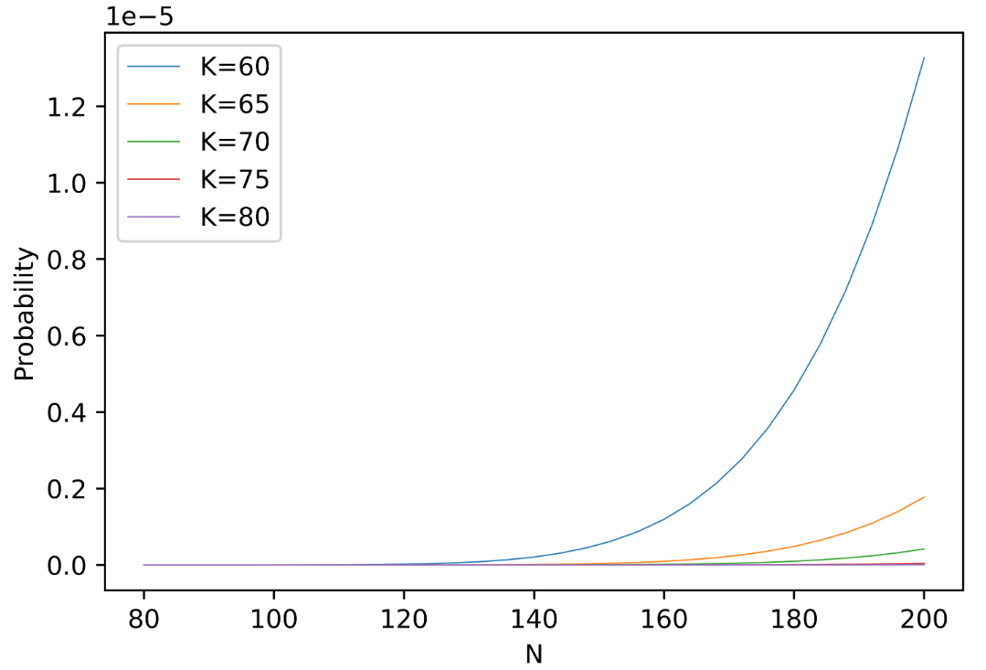
Figure 2: A random exploration strategy works with fairly high probability if the solution can be achieved in a small distance traveled from the origin. As can be seen above, as the distance from origin $K$ increases, the probability of success decreases exponentially for the same episode length $N$. See A.2 in the Appendix for derivation.

Information Content-based Exploration (ICE) introduces an intrinsic reward that maximizes information gain in the state space. In each episode of interaction with the environment, we aggregate trajectory statistics to approximate the entropy of the state visitation distribution and reward the agent for relative improvements to this measure. This approach formalizes the exploration process as seeking low-density states but can easily accommodate prior knowledge of the environment by replacing entropy with KL-divergence to a desired state density, similar to (Lee et al., 2020).

We run several experiments comparing ICE’s performance against RND and CDL using A3C (Mnih et al., 2016) as our base RL algorithm to show that ICE significantly outperforms RND and CDL in various environments. We also observe that ICE exploration exhibits trajectories akin to depth-first search. In most environments, this offers the best opportunity to find extrinsic rewards, where the agent must decisively commit to a path through the environment rather than dithering locally via action entropy. Finally, we discuss extensions to our approach that generalize to continuous state spaces by maximizing information content on a hashed latent space extracted from an auto-encoder architecture.

2 Background

We briefly cover A3C in section 2.1, and introduce the Source Coding Theorem which provides the theoretical justification for using entropy in the state space for exploration in ICE. In 2.3 and 2.4, we cover Curiosity Driven Learning and Exploration by Random Network Distillation algorithms.

2.1 Actor Critic Algorithm

We consider a parametric policy $\pi_{\theta}\in\Pi:=\{\pi_{\theta}:\theta\in\Theta\}$ interacting with a discounted Markov Decision Process $\mathcal{M}=$($\mathcal{S},\mathcal{A},\gamma,\mathcal{P},r$). At each time step $t$, the policy outputs an action $a_{t}\sim\pi_{\theta}(\cdot|s_{t})$ that leads to the next state $s_{t+1}$ according to the transition kernel $\mathcal{P}(s_{t+1}|s_{t},a_{t})$. The environment also provides an extrinsic reward $r_{t}\sim(s_{t},a_{t})$. The objective is to maximize the expected discounted cumulative reward $\mathcal{J}(\pi)=\mathbb{E}_{\pi}(\sum_{t=0}^{\mathcal{T}}\gamma^{t}r_{t})$. The critic is an auxiliary model with parameters $\phi\in\Phi$ that reduces the variance of the policy gradient by approximating the value function: $\hat{V}_{\phi}^{\pi}(s_{t})\approx\mathbb{E}_{\pi}[\sum_{k}\gamma^{k}r_{t+k+1}|s_{t}]$.

The Actor-Critic method maximizes the objective $\mathcal{J}$ by optimizing the model’s weights based on value loss, policy loss, and entropy loss, which have the form

$$\begin{split}L_{value,t}&=\alpha_{value}(r_{t}+\gamma V_{\phi}(s_{t+1})-V_{\phi}(s_{t}))^{2}\\ L_{policy,t}&=\alpha_{policy}(-A_{t}\log\pi_{\theta}(a_{t}|s_{t}))\\ L_{entropy,t}&=\alpha_{entropy}(-\mathbb{H}(\pi_{\theta}(\cdot|s_{t})))\end{split}$$ (1)

where $\alpha_{value},\alpha_{policy},\alpha_{entropy}$ are the weight coefficients of the three losses, $\pi_{\theta}(a_{t}|s_{t})$ is the probability of the selected action policy, $\mathbb{H}(\pi_{\theta}(\cdot|s_{t}))$ is the entropy of the policy.
In addition, $k$-step Advantage estimate $A_{t}$ is defined to be

$$A_{t}=\sum_{i=0}^{k-1}(\gamma^{i}r_{t+i})+\gamma^{k}V_{\phi}(s_{t+k})-V_{\phi}(s_{t})$$ (2)

In the case where the intrinsic reward is present, the reward $r_{t}$ is the weighted sum of intrinsic and extrinsic reward,

$$r_{t}=r^{extrinsic}_{t}+\beta r^{intrinsic}_{t}$$ (3)

where $\beta$ is the weight coefficient of the intrinsic reward.

The k-step state distribution induced by a policy $\pi$ is given by:

$$d_{k,\pi}(s) =\mathbb{E}_{\begin{subarray}{c}s_{1}\sim\rho_{0}(\cdot)\\ a_{t}\sim\pi(\cdot|s_{t})\\ s_{t+1}\sim\mathcal{P}(\cdot|s_{t},a_{t})\end{subarray}}[\frac{1}{k}\sum_{t=1}^{k}1(s_{t}=s)]$$ (4)

2.2 Source Coding Theorem

Given a list of discrete elements $L=\{l_{0},l_{1},...,l_{t}\}$, $l_{i}\in\mathbb{R}^{1}$, the Source Coding Theorem states that $L$ can be compressed into no less than $H^{L}_{t}\times(t+1)$ bits, where $H^{L}_{t}$ is the entropy of $L$ up to step $t$.

Theorem 2.1 (Source Coding Theorem (Shannon, 1948), $D=1$).

A single random variable (D=1) with entropy $H$ can be compressed into at least $H$ bits without risk of information loss.

We note that the joint entropy is sub-additive, with equality when the random variables are independent (Aczel et al., 1974):

$$H(X_{1},...,X_{n})\leq\sum_{i}H(X_{i})$$ (5)

We also note that up to a constant, the entropy of a discrete random variable $X:\mathcal{X}\to\{1,...,K\}$ distributed according to $p$ is given by $-D_{KL}(p,\mu)$ where $\mu$ is the uniform distribution on $\mathcal{X}$, and $D_{KL}$ is the KL divergence:

$$D_{KL}(p,\mu) =\sum_{k=1}^{K}p(X=k)log\frac{p(X=k)}{K^{-1}}$$ (6)

$$=logK+\sum_{k=1}^{K}p(X=k)logp(X=k)$$ (7)

$$=logK-\mathbb{H}(X)$$ (8)

Hence, maximizing the state distribution entropy is equivalent to minimizing the reverse KL to the uniform distribution over state.

2.3 Curiosity Driven Learning (CDL)

This branch of exploration provides an intrinsic reward based on the agent’s familiarity with the current state; curiosity-driven Exploration by Self-supervised Prediction (Pathak et al., 2017) is one of the popular approaches. It formulates the intrinsic reward by using three neural networks to estimate state encoding, forward dynamics, and inverse dynamics. The first neural network $f_{encode}(s)$ encodes $s_{t}\mapsto g_{t}$ and $s_{t+1}\mapsto g_{t+1}$. Then a second neural network $f_{forward}(g_{t},a_{t})$ estimates the next state encoding $\hat{g}_{t+1}$. Lastly, the third neural network $f_{inverse}(g_{t},g_{t+1})$ estimates the transition action distribution $\hat{a_{t}}$. The training loss and intrinsic reward have the form

$$\begin{split}L_{forward_{t}}&=\alpha_{forward}MSE(g_{t+1}-\hat{g_{t+1}})\\ L_{inverse_{t}}&=\alpha_{inverse}CrossEntropy(\hat{a_{t}},a_{t})\\ r_{intrinsic_{t}}&=\beta L_{inverse_{t}}\end{split}$$ (9)

The agent will naturally favor states that it cannot accurately predict the transition action from $s_{t}$ to $s_{t+1}$.

2.4 Exploration by Random Network Distillation (RND)

Exploration by Random Network Distillation (Burda et al., 2018b) follows the same design philosophy as Curiosity Driven Learning. It formulates the intrinsic reward by using two neural networks. The first neural network $f_{random}(s)$, encodes $s_{t}\mapsto g_{t}$. It is randomly initialized and will not get updated. The second neural network $f_{encode}(s)$, encodes $s_{t}\mapsto\hat{g}_{t}$. The training loss and intrinsic reward have the form

$$\begin{split}&L_{encode_{t}}=\alpha_{encode}MSE(g_{t+1},\hat{g_{t+1}})\\ &r_{intrinsic_{t}}=\beta L_{inverse_{t}}\end{split}$$ (10)

where $\alpha_{encode}$ and $\beta$ are coefficients. This method encourages the agent to explore in states where $f_{encode}$ cannot accurately predict the random encoding.

3 Information Content-based Exploration (ICE)

3.1 Motivation

While interacting with the environment, we view the t-step state sequence $s_{1},...,s_{t}$ as a 1-sample Monte-Carlo approximation to the t-step state distribution $\hat{d}_{t,\pi}(s)\approx d_{t,\pi}(s)$ induced by the agent $\pi$. Supposing that our state space $\mathcal{S}$ is isomorphic to $\textbf{K}^{D}:=\{1,2,..,K\}^{D}$, then we can compute the empirical entropy of the t-step state sequence $\hat{d}_{t,\pi}(s)$:

$$\mathbb{H}(\hat{d}_{t,\pi}(s))=-\sum_{x\in\textbf{K}^{D}}\hat{p}(x)log\hat{p}(x)$$ (11)

in $\mathcal{O}(t\cdot K^{D})$. For computational reasons, we view each state trajectory as composed of $D$ independent state elements (e.g., frames of a video made up of $D$ pixels) which reduces the complexity to $\mathcal{O}(t\cdot K\cdot D)$:

$$\sum_{x\in\textbf{K}^{D}}\hat{p}(x)log\hat{p}(x)\approx\sum_{d\in D}\sum_{k\in\textbf{K}}\hat{p}(x_{d}=k)log\hat{p}(x_{d}=k)$$ (12)

We provide an intrinsic reward to the agent based on the relative improvement of this measure across time steps. Thus, we optimize for the approximate derivative of state entropy. We view several benefits to using the relative improvement measure:

• Intrinsic stochasticity (e.g. persistent white noise) has high Shannon entropy but low fundamental information content (since the data is non-compressible). The relative improvement measure nullifies such entropy sources.

• Let $\delta_{t}\geq 0$ be the sub-additivity gap introduced by assuming our state-sequence $s_{1},...,s_{t}$ is independent. If $\delta_{t}$ is relatively constant across time then the relative improvement measure cancels out the overestimation of state entropy introduced by our independence assumption.

In 3.2 we give an efficient algorithm for computing the intrinsic ICE reward, then, in 3.4 we discuss a principled approach to state discretization, which enables us to compute ICE in continuous state spaces.

3.2 Algorithm

Let us define a trajectory, $X_{t}$, to be the list of states collected from the same episode up to step $t$, $X_{t}=[s_{0},s_{1},...,s_{t}]$, where each state $s_{t}$ is a collection of state elements, $s_{t}=[s_{t}^{0},s_{t}^{1},...,s_{t}^{D-1}]\in\mathbb{R}^{D}$. To collect the total information in a trajectory, we first calculate the information content received over each state element in a trajectory.

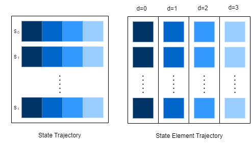
Figure 3: A trajectory is the collection of all states traversed by the agent in sequence. State element trajectory is the collection of elements from the same position in all states in a trajectory.

Consider an arbitrary state element $d$ in a trajectory up to step $t$, $X^{d}_{t}=[s_{0}^{d},s_{1}^{d},...,s_{t}^{d}]$. We can calculate the count for each unique value within $X^{d}_{t}$.

$$q^{d}_{t}=CountUnique(X^{d}_{t})$$ (13)

Next, we can calculate the probability of each unique value occurrence within $X^{d}_{t}$.

$$p^{d}_{t}=\frac{q^{d}_{t}}{t+1}$$ (14)

For example, if $X^{d}_{t=4}=[a,a,b,a,c]$, then $q^{d}_{t=4}=[3,1,1]$ and $p^{d}_{t=4}=[3/5,1/5,1/5]$.

We can then obtain the entropy for $X^{d}_{t}$ by applying Shannon’s entropy to $p^{d}_{t}$.

$$H^{d}_{t}=Entropy(p^{d}_{t})=-\sum_{k}p^{d}_{t}[k]\log_{2}p^{d}_{t}[k]$$ (15)

$H^{d}_{t}$ measures the information content of the $d^{th}$ state element trajectory. The information content of the full trajectory can be calculated by summing over all state elements.

$$H_{t}=\sum_{d}H^{d}_{t}$$ (16)

We then denote $r^{intrinsic}_{t}$ as

$$r^{intrinsic}_{t}=H_{t}-H_{t-1}$$ (17)

Intuitively, $r^{intrinsic}_{t}$ represents the amount of additional information $s_{t}$ brings to the trajectory $[s_{0},s_{1},...,s_{t-1}]$. Note that $\sum r^{intrinsic}_{t}=H_{T}$, which is the total information content of the entire trajectory. A numerical example of $r^{intrinsic}_{t}$ calculation can be found in Appendix A.3.

Algorithm 1 Information Content-based Intrinsic Reward

  Input: Model $M$

  repeat

     Input: state $s_{0}$, $H_{last}\leftarrow 0$, $t\leftarrow 0,\ done\leftarrow False$

     Input: unique count dictionary $q$

     $q\leftarrow Update(q,s_{0})$, from Eq.13

     $H_{last}\leftarrow CalculateICE(q)$, from Eq.16

     while not $done$ do

        $a_{t}\leftarrow M(s_{t})$

        $s_{t+1},r^{extrinsic}_{t},done\leftarrow env.step(a_{t})$

        $q\leftarrow Update(q,s_{t+1})$

        $H_{current}\leftarrow CalculateICE(q)$

        $r^{intrinsic}_{t}\leftarrow H_{current}-H_{last}$

        $r_{t}\leftarrow r^{extrinsic}_{t}+\beta r^{intrinsic}_{t}$

        $H_{last}\leftarrow H_{current}$

        $t\leftarrow t+1$

     end while

     Update model $M$

  until Model $M$ Converge

This formulation of the $r^{intrinsic}$ requires no estimation, as it can be calculated directly from the trajectory of states. By maintaining count arrays of size $D\times K$, we can efficiently implement Alg. 1 using vectorized CPU or GPU operations. See the supplementary Material for our implementation.

3.3 State Exploration vs Action Exploration

ICE is a state space exploration algorithm and assumes the environment to be an observable Markov Decision Process. This assumption is necessary because ICE measures the information content of the observable state trajectory.

ICE encourages the agent to efficiently explore the trajectory containing the most information content at the cost of disincentivizing the agent from pursuing trajectories with low information. Therefore, ICE offers no guarantee that every state in the decision process will be visited. On the other hand, action space exploration (Eq.1) encourages the agent to take actions based on uniform distribution. Albeit inefficient, it does guarantee that the agent will eventually visit all states in an environment.

State space exploration is fundamentally different than action space exploration. They are complements to each other. In the case where the agent is driven only by the action of space exploration, the agent can reach all reachable states, but the expected amount of time required can be very long. On the other hand, an agent driven only by state space exploration can reach more distinct states in significantly less amount of time, but it is no longer guaranteed to reach all reachable states. The probability of reaching a reward is proportional to the percent of all possible states reached. As shown in Fig.4, The agent with high state exploration and low action exploration can potentially reach rewards in a shorter amount of time but with a possibility that it may never reach all the rewards. Therefore, it is important to balance the weighting of these two types of explorations in order to explore optimally, illustrated in (Fig.4) and 4.3.

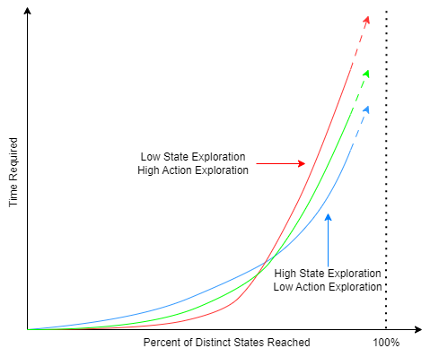
Figure 4: As we increase the action exploration and decrease the state exploration, it takes significantly longer to reach the same amount of distinct states (blue line). In the case where we decide to only apply state exploration, the agent will be able to efficiently follow the trajectory with very rich information content, at the cost of never visiting states in the low information content trajectories. As a result, such an agent will almost never reach all the states (red line).

3.4 ICE in a Learned Latent Space

A trajectory’s information content depends on how we choose to discretize the state space; naturally, different discretization methods will change the absolute information content. Selecting the appropriate discretization is only possible with prior knowledge of the environment. We propose to address this by using an auto-encoder to learn a compressed, low-dimensional discrete representation upon which information is maximized. Computing ICE on the latent manifold decouples the ICE formulation from the dimensionality of the observation space. The information bottleneck principle (Tishby et al., 1999) allows us to trade between sufficiency and minimality in our discrete representation.

Since the KL divergence is parameterization-invariant, we can be sure that insofar as our auto-encoder learns an invertible representation of the state space, computing ICE in latent space should lead to desirable exploration behaviour as in discrete settings. We validate this procedure in 4.4.

3.4.1 Motivation

We put $\mathcal{D}=\{d:\mathcal{S}\to\mathbb{R}_{\geq 0}\}$ to be the set of distributions over the state space, and we consider functionals $\mathcal{R}(\cdot)$ that describe how desirable a given state distribution is. If we take $\mathcal{R}(d)=\mathbb{H}(d)$ on a discrete space we recover the formulation of 3.2. More generally, if we have some target distribution $d^{*}$, we can consider the reverse KL:

$$\mathcal{R}_{d^{*}}(\cdot)=D_{KL}(\cdot,d^{*})$$ (18)

We consider the family of measurable surjective maps: $\mathcal{F}:\{\mathcal{S}\to\mathcal{Z}\}$, where $\mathcal{Z}$ is a discrete space of dimensions $k\leq dim(\mathcal{S})$. The inverse set map partitions $\mathcal{S}$, giving rise to the following relation:

$$d_{1}\sim^{f}d_{2}\iff f_{*}(d_{1})=f_{*}(d_{2})$$ (19)

where $f_{*}()$ is the push-forward measure on $\mathcal{Z}$. We let:

$$[\mu]_{f}=\{d\in\mathcal{D}:d\sim^{f}\mu\}=f^{-1}(Unif_{z})$$ (20)

denote the subset of state distributions whose projection onto $\mathcal{Z}$ by $f$ result in the uniform distribution.

Then we put:

$$\mathcal{R}_{f}(\cdot)=D_{KL}(\cdot,[\mu]_{f})=\mathbb{H}[f(\cdot)]$$ (21)

In words, we think about $f$ as a filter that represents various invariants on our state space $\mathcal{S}$. All state distribution that map uniformly on $\mathcal{Z}$ by $f$ are considered equally desirable, and we reward trajectories with high information content from the lens of $f$.

3.4.2 Learning the latent Representation

We let $\mathcal{Z}$ arise as a discrete bottleneck $\mathcal{S}\to^{e}\mathcal{Z}\to^{d}\mathcal{S}^{\prime}$ from aiming to reconstruct state as best as possible, thereby inducing a representation $\mathcal{Z}$ that maximizes mutual information with $\mathcal{S}$. A smoothly parameterizes encoder (e.g. neural network) will ensure that similar states get mapped to similar codes. Hence, maximizing information content on $\mathcal{Z}$ will further encourages diverse trajectories on $\mathcal{S}$.

To discretize the latent space, we use locality sensitive hashing (LSH) (Zhao et al., 2014). LSH is helpful because state dimensions that are highly coupled (from an information-theoretic view), will be hashed to the same latent code by our auto-encoder whose projections to a lower dimension filter out small perturbations. On the other hand, a novel experiences will project to different latent subspace and thus will be prescribed a unique hash code. This approach decouples the ICE procedure from the state-space dimensionality, and can be directly applied to continuous spaces.

We follow the discretization pipeline similar to (Tang et al., 2017), using a Simhash (Charikar, 2002) scheme with a auto-encoder. Namely, for an encoder $e:\mathcal{S}\to\mathbb{R}^{D}$, a decoder $d:\mathbb{R}^{D}\to\mathcal{S}$, fixed stochastic matrix $A\in\mathbb{R}^{k\times D}$ with $A_{ij}\sim\mathcal{N}(0,1)$, we retrieve the discrete latent code for state $s$ according to:

$$z(s)=sgn(A\sigma(\mathcal{U}_{(-a,a)}+e(s)))\in\{-1,1\}^{k}$$ (22)

where $\sigma(\cdot)$ denotes element-wise application of the sigmoid function, and $\mathcal{U}_{(-a,a)}$ is the injection of uniform noise to force the latent space to behave discretely (Hubara et al., 2016), (Maddison et al., 2016).

The encoder and decoder are parameterized by convolution neural networks, jointly trained with the reinforcement learning policy on a lagged updated schedule to ensure the latent codes are stable while retaining the ability to adjust based on exploratory progress of the agent. The auto-encoder optimizes a log likelihood term and an auxiliary loss that ensures unused latent bits take on an arbitrary binary value, preventing spurious latent code fluctuations (Tang et al., 2017):

$$\mathcal{L}(\{s_{i}\}_{i=1}^{N})=-\frac{1}{N}\sum_{i=1}^{N}[logp(s_{i})-\newline \frac{\lambda}{K}\sum_{i=1}^{D}g(s_{i})]$$ (23)

$$g(s_{i}):=min\{(1-e(s_{i}),e(s_{i})\}$$ (24)

The algorithm for running ICE on a learned latent space is given in Alg.2. We note that using learned hash codes involves minimal changes to the base ICE algorithm, requiring only that (1) states pass through the encoder and SimHash prior to computing ICE reward, and (2) a buffer of approximately reconstructed state trajectories is stored to periodically updating the auto-encoder based on Eq.23.

Algorithm 2 Information Content-based Intrinsic Reward in Learned Latent Space

  Input: Model $M$, Encoder $e:\mathcal{S}\to\mathbb{R}^{D}$, Decoder $d:\mathbb{R}^{D}\to\mathcal{S}$, Fixed Gaussian matrix $A\in\mathbb{R}^{k\times D}$. Buffer $\mathcal{B}$

  repeat

     Input: state $s_{0}$, $H_{last}\leftarrow 0$, $t\leftarrow 0,\ done\leftarrow False$

     Input: unique count dictionary $q$

     $z_{0}\leftarrow Encode(s_{0},e,A)$, from Eq.22

     $\hat{s_{0}}\leftarrow Decode(s_{0},z_{0},d)$

     $\mathcal{B}\leftarrow(s_{0},z_{0},\hat{s_{0}})$ add to buffer

     $q\leftarrow Update(q,z_{0})$, from Eq.13

     $H_{last}\leftarrow CalculateICE(q)$, from Eq.16

     while not $done$ do

        $a_{t}\leftarrow M(s_{t})$

        $s_{t+1},r^{extrinsic}_{t},done\leftarrow env.step(a_{t})$

        $z_{t+1}\leftarrow Encode(s_{t+1},e,A)$, from Eq.22

        $\hat{s_{t+1}}\leftarrow Decode(s_{t+1},z_{t+1},d)$

        $\mathcal{B}\leftarrow(s_{t+1},z_{t+1},\hat{s_{t+1}})$ add to buffer

        $q\leftarrow Update(q,z_{t+1})$

        $H_{current}\leftarrow CalculateICE(q)$

        $r^{intrinsic}_{t}\leftarrow H_{current}-H_{last}$

        $r_{t}\leftarrow r^{extrinsic}_{t}+\beta r^{intrinsic}_{t}$

        $H_{last}\leftarrow H_{current}$

        $t\leftarrow t+1$

     end while

     Update model $M$

     if iteration mod $ae_{update}=0$ then

        update encoder $e$ and decoder $d$ with data from buffer $\mathcal{B}$ according to Eq. 23

     end if

  until Model $M$ Converge

4 Experiment

We compare information content based intrinsic reward with several other methods from the literature described in Section $2$. The selected environments include Grid-World, along with a group of sparse reward Atari games. All of the environments in this experiment are reduced to $40\times 40$ dimensionality and discretized using 255 gray scale range. We use a single convolution neural network with LSTM layers and seperate value and policy heads to parameterize the actor and critic. Details are given in A.5.

The unique count matrix $Q$ (Eq.13) is preset to be $Zeros(40,40,C)$ at the beginning of each trajectory, where $C$ is the number of unique values for each pixel. The algorithm will dynamically update the matrix $P$ and then calculate the trajectory information content after each step.

4.1 Grid-World

The state space for grid world is a $40\times 40$ grid (Fig.8 left). The agent starts at the (0,0) position and it can take action from $\{up,down,left,right\}$. The grid visited by the agent is labeled as 1, otherwise 0, the extrinsic reward by the environment is always 0, and the environment terminates after 400 steps.
As shown in (Fig.5), the agent is able to explore up to 300 distinct states in every trajectory with ICE enabled, which is significantly more than the case when ICE is disabled. The trajectory information content also increases as the number of distinct states increases.

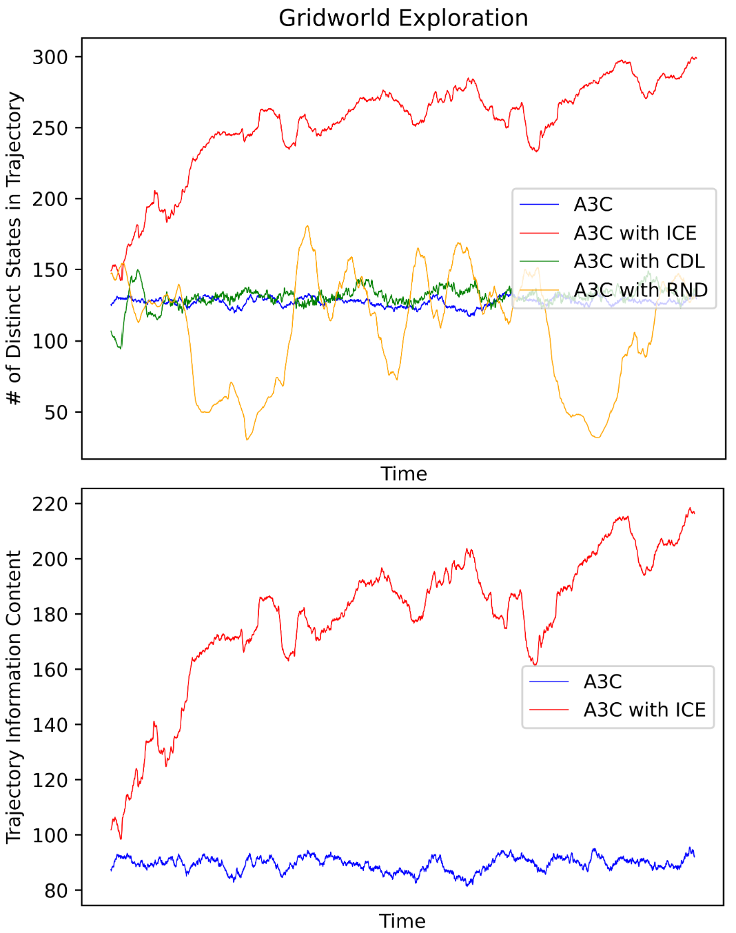
Figure 5: ICE motivates agent to reach a significantly higher number of distinct states which is correlated with an increase in information content. Measured in a no-reward grid-world environment.

4.2 Atari

We compare ICE with A3C, CDL, and RND on several environments from Atari.
Firstly we compare the methods of Pong and Breakout, Fig.6. The performance of ICE is slightly worse than A3C. This is because these two environments both have very rich reward systems. They do not necessarily require an exploration signal in order to solve. In these environments, the intrinsic rewards are noise rather than a signal to the model. Nonetheless, ICE will not degrade the performance by a lot as long as we keep it to a relatively small magnitude. As a result, ICE is able to solve both environments efficiently.

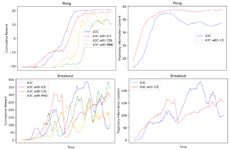
Figure 6: Performance on simple Atari Environments, cumulative reward (left), information content (right)

The second set of environments is Pong with Sparse Reward, Super Mario, and Montezuma, Fig.7. These are challenging for RL algorithms due to their extremely sparse reward system. In Pong with Sparse Reward, all of the rewards were accumulated and provided to the model at the last step. In Super Mario, the agent gets no reward during learning and gets properly rewarded during evaluation (see A.4 for more details). In Montezuma, the agent will only get a positive reward if the character reaches a key. These environments require the agent to precisely follow an action trajectory in order to solve the problem. In all cases, the ICE agent outperformed the base A3C agent. The learning for ICE is also very efficient as focuses on efficiently exploring the state space. ICE also displays interesting behaviors in the Montezuma Revenge environment. In the early stages, the agent focuses on exploring distinct states as it receives no rewards. As soon as it lands on a key, it quickly shifts its focus towards maximizing the extrinsic reward. Simultaneously, the intrinsic reward quickly degrades. Shortly after, the agent tries to regain the intrinsic reward while still being able to reach the key. As shown in the right column of Fig.6,7, ICE is very correlated with the environment’s reward system, because Atari games such as Pong and Breakout have deterministic and observable state spaces, which gives a clear measure of information content using ICE. In general, ICE is a very robust exploration method because it is not very sensitive to hyper-parameters and is not prediction-based.

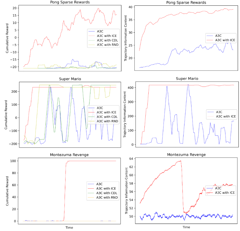
Figure 7: Performance on Sparse Reward Environments, cumulative reward (left), information content (right).

4.3 Grid-World with Wall

This is a special case of the Grid-World to illustrate the idea of 3.3. The basic setup is the same as described in 4.1, with differences shown in Fig.8. The block of the wall marked in black represents states the agent cannot visit. On top of this, the grids marked in blue are unobservable, as they will always be filled with 0, and the grids marked in yellow are standard (turns to 1 if visited, else 0). The agent will get a positive reward and terminate the game if it has reached the green grid. The agent with ICE is efficiently exploring yellow grids, but it is having trouble exploring blue grids and cannot land on the green grid. This is because the agent quickly converged to take the path in yellow grids, as it can generate higher information content compared to a path in blue grids. On the other hand, the agent without ICE is able to land at the green grid after a while of random search (Fig.9). This is a limitation of ICE that can be overcome by simply including action exploration.

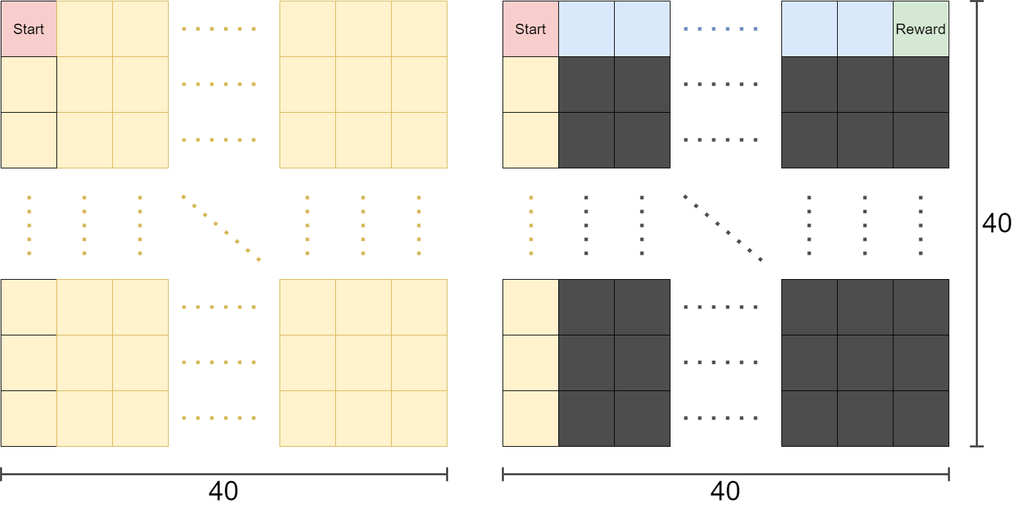
Figure 8: Setup of grid world (left) and grid world with wall (right). The agent will always start at the top-left corner. Yellow grids are observable, turn to 1 when visited. Blue grids are non-observable, always filled with 0. Black grids are walls that agents cannot step into. Green grid gives a positive reward to the agent.

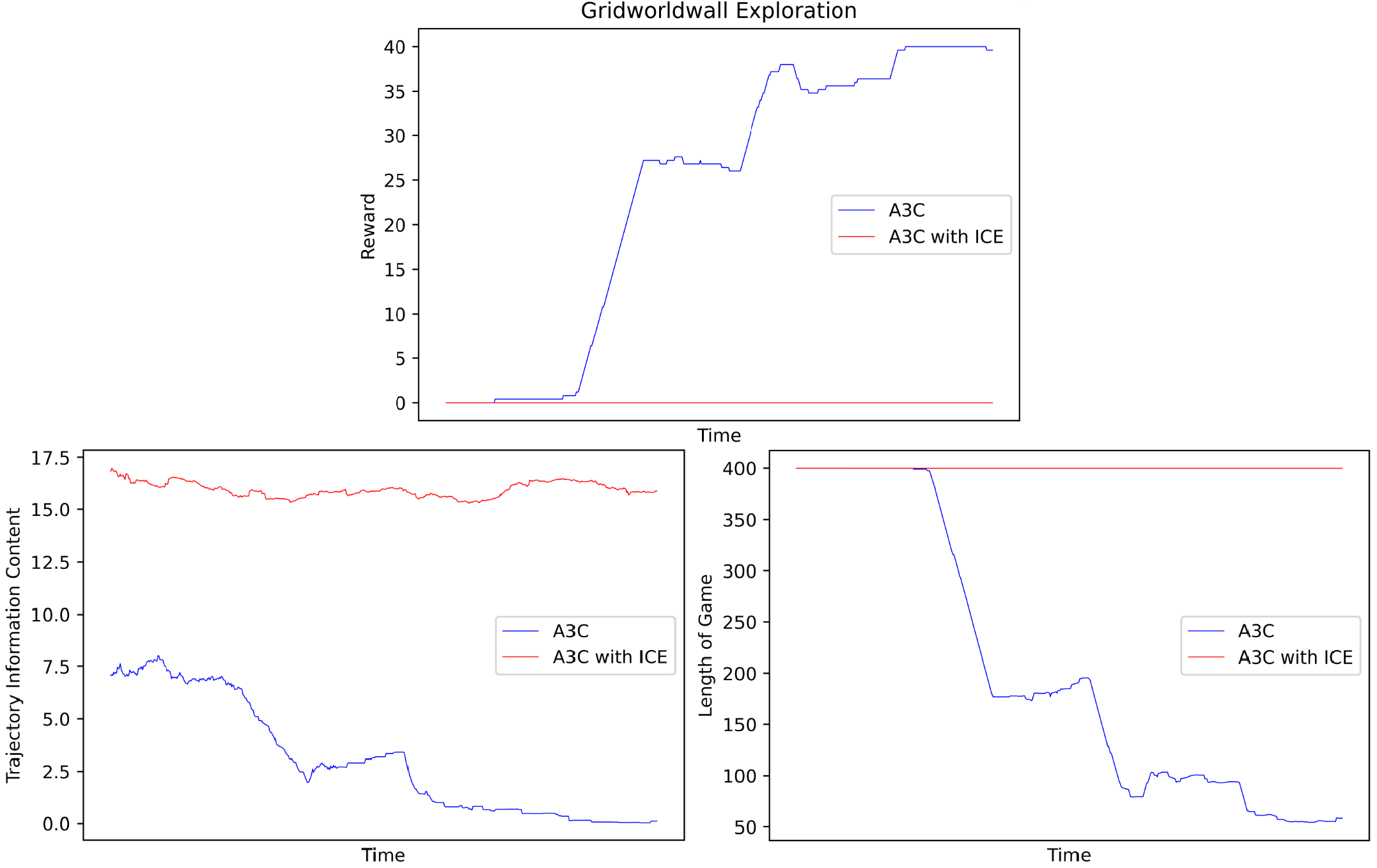
Figure 9: The agent with ICE is exploring efficiently in yellow grids but is not able to make it to the green grid. The agent without ICE finds the green grid after a few rounds of random search and quickly converges to this path.

4.4 ICE in a Learned Latent Space

We evaluate how well ICE performs when computed on a learned latent space, following the procedure of 3.4.2, on several environments including Pong, Breakout, Montezuma’s revenge and Starpilot. The encoder consists of 3 convolution blocks followed by a linearity outputting a $128$-dimensional dense representation which is hashed into $k=16$-dimensional latent codes. The decoder consists of 3 deconvolution blocks. We use $\lambda=0.5$ for the auxiliary auto-encoder loss, and update the auto-encoder every 3 updates of the base policy. This architecture is inspired by the representation learning stack from (Tang et al., 2017), which aim to achieve high reconstruction accuracy to help stabilize the learned latent space, and thereby make our ICE reward more consistent.

The extrinsic reward learning curves are shown in 3.4.2. We observe that working in a compressed representation can be beneficial, even for state spaces that are already discrete (e.g. images). In Pong and Starpilot, ICE in latent space improves the speed of learning, suggesting that the bottlecked representation helps regularize against sporadic noise in our state trajectories.

In Montezuma’s revenge, optimizing for ICE in latent space exhibits asymptotically better extrinsic rewards, suggesting that maximizing information content on the compressed representation is better able to capture semantically meaningful subspaces worth exploring.

We believe that these initial results are promising, and we are motivated to further experiment with ICE rewards on various representation spaces.

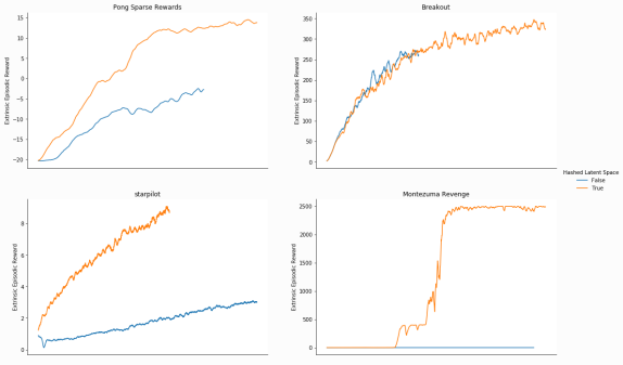
Figure 10: Comparing performance of ICE reward in learned latent space (orange) vs. ICE reward directly on uniformly discretized pixels (blue). Optimizing the ICE reward on the learned latent space improves sample-efficiency in Pong, Starpilot and Montezuma.

5 Conclusion

We have introduced a new intrinsic reward based on the information content of trajectories measured using Shannon’s Entropy. Our method is amenable to vectorized implementation and has shown robustness in various observable MDP’s. ICE motivates the agent to explore diversified trajectories, thereby increasing its sample-efficiency in sparse environments where the probability of receiving a reward is directly proportional to the number of distinct visited states. We discussed a discretization scheme 3.4 based on locality sensitive hashing that maximizing information content on a compressed latent space, generalizing ICE reward to continuous state spaces. We also examined the limitations of motivating agents to traverse trajectories with a large number of distinct states in 4.3.

6 Future Work

The idea of this work is loosely related to depth-first search (DFS). By analogy, action state exploration is a cyclic breadth-first search (BFS). We believe that there is opportunity to improve ICE by dynamically shifting between DFS and BFS behaviour as the agent interacts with the environment. We also posit that changing the formulation to incorporate information across multiple episodes can yields better results. For example, we can maximize information content of the current trajectory while minimizing the mutual information with previous experience; we leave this to future work. Finally, we’ve observed promising results using ICE on a learned latent representation. In future work, we wish to further validate this process by evaluating it using different representations such as the successor representation (Machado et al., 2023), and rigorously testing sensitivity to hash-dimension on continuous spaces.

Software and Data

We include an A3C and a PPO implementation of ICE in the Supplementary Material.

Appendix A Appendix

A.1 Hyperparameters

Table 1: Hyperparameters used in our experiments.

	gridworld	gridworldwall	Pong	Montezuma	Mario
lr	$10^{-4}$	$10^{-4}$	$10^{-4}$	$10^{-4}$	$10^{-4}$
gamma	0.99	0.99	0.99	0.99	0.99
$\alpha_{value}$	0.5	0.5	0.5	0.5	0.5
$\alpha_{policy}$	1.0	1.0	1.0	1.0	0.5
$\alpha_{entropy}$	0.01	0.01	0.01	0.01	0.01
$\beta$	0.5	0.5	0.5	1.0	0.1

A.2 1-D Random Walk Analysis

We want to show by calculation that it is very unlikely an agent can end at equal or larger than $K$ distances away from the origin after taking $N$ random steps in a 1-dimension grid. As shown in Fig.11, the agent starts at the 0 position and takes action from left, right randomly. Define the probability of an agent end at equal or larger than $K$ distances away from the start position after taking $N$ random steps to be $P_{k}^{N}$.

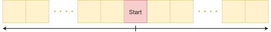
Figure 11: Setup of a 1-D random walk grid. The agent starts at the 0 position and takes action from left, right randomly.

In the case where $N\geq K$, it follows from the binomial distribution,

$$P_{k}^{N}=\sum_{i=\left\lceil\frac{K+N}{2}\right\rceil}^{N}\binom{N}{i}\left(\frac{1}{2}\right)^{N}$$ (25)

For large $N$ and $K\ll N$, we can apply Stirling’s Formula (Dutka, 1991) to simplify the calculation.

A.3 More examples

We will illustrate $r^{intrinsic}_{t}$ by an example. Consider a simple grid world environment with dimension $1\times 4$. Every grid begins with value $0$, and changes to 1 on visitation. The agent starts at the leftmost grid. The agent has $2$ possible actions (left, right). The environment itself provides no reward, $r^{extrinsic}_{t}=0,\forall\ t$. The game terminates after $3$ steps. Let’s consider an example trajectory, where the actions are $left,right,right$.

$$s_{0},s_{1},s_{2},s_{3}=[1,0,0,0],[1,0,0,0],[1,1,0,0],[1,1,1,0]$$ (26)

Then the trajectory for each state variable up to $t=4$ is

$$X^{d=0}_{t=3},X^{d=1}_{t=3},X^{d=2}_{t=3},X^{d=3}_{t=3}=[1,1,1,1],[0,0,1,1],[0,0,0,1],[0,0,0,0]$$ (27)

The count unique and probability occurrence vector for each state variable up to $t=3$ is

$$\begin{split}&q^{d=0}_{t=3},q^{d=1}_{t=3},q^{d=2}_{t=3},q^{d=3}_{t=3}=[0,4],[2,2],[3,1],[4,0]\\ &p^{d=0}_{t=3},q^{d=1}_{t=3},q^{d=2}_{t=3},q^{d=3}_{t=3}=[0/4,4/4],[2/4,2/4],[3/4,1/4],[4/4,0/4]\end{split}$$ (28)

The total information content of this trajectory can be calculated as

$$\begin{split}&H^{d=0}_{t=3},H^{d=1}_{t=3},H^{d=2}_{t=3},H^{d=3}_{t=3}=0,1,0.81,0\ bits\\ &H_{t=3}=\sum H^{d}_{t}=1.81\ bits\\ \end{split}$$

Other $H_{t}$ where $t\in[0,1,2]$ can be calculated through the same method, where $H_{t=0}=0,H_{t=1}=0,H_{t=2}=0.92$. Lastly, the intrinsic reward is

$$r^{intrinsic}_{t=3}=H_{t=3}-H_{t=2}=0.89\ bits$$ (29)

Note that the agent can increase its information content by visiting more distinct grids within the trajectory, and the maximum is achieved when all grids have been visited exactly once within $N$ steps. The grid world environment is a very representative environment for many sparse reward environments. They are similar in a way that their exploration objective can all be described as increasing the probability of reaching a non-zero reward state by exploring more distinct states.

A.4 Super Mario Reward System

The extrinsic reward for the Super Mario environment is always 0 during learning, and the extrinsic reward during evaluation is as follows (Kauten, 2018),

$$\begin{split}&velocity_{t}=position_{t}-position_{t-1}\\ &clock_{t}=time_{t-1}-time_{t}\\ &death_{t}=0\ if\ alive\ else\ -15\\ &r^{extrinsic}_{t}=velocity_{t}+clock_{t}+death_{t}\end{split}$$ (30)

A.5 Neural Network Architecture

The neural network is designed to be a combination of 4 convolution, 1 LSTM, and 2 linear layers (Fig.12). The LSTM layer is important here to give the model a sense of the states it has traveled so far in a trajectory.

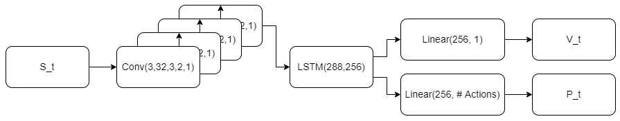
Figure 12: Neural Network Structure

A.6 Locality Sensitive Hashing

We consider locality sensitive hashing. A family of hash functions $\mathcal{H}=\{h:\mathcal{S}\to\mathbb{Z}\}$ is locality sensitive for a similarity function s: $\mathcal{S}\times\mathcal{S}\to\mathbb{R}$ if a hash function $h\sim\mathcal{H}$ randomly sampled from the family satisfies:

$$d(s_{1},s_{2}) \leq R\implies p(h(s_{1})=h(s_{2})\geq P_{1})$$ (31)

$$d(s_{1},s_{2}) \geq C\cdot R\implies p(h(s_{1})=h(s_{2}))\leq P_{2}$$ (32)

for some constants $C>1,R>0$ and for probabilities $P_{1},P_{2}\geq 0$. In other words, points close together are hashed to the same value with high probability, and dissimilar points are unlikely to collide in hash. Implicit in this assumption is that $(\mathcal{S},d)$ form a valid metric space.

Locality sensitive hashing enables us to map a continuous, high dimensional state space into a compressed latent space such that similar points in state space map to similar latent codes.

References

- Achiam & Sastry (2017) Achiam, J. and Sastry, S. Surprise-based intrinsic motivation for deep reinforcement learning. arXiv preprint arXiv:1703.01732, 2017.
- Aczel et al. (1974) Aczel, J., B.Forte, and NG, C. T. Why the shannon and hartley entropies are natural. Applied Probability Trust, 6:131–146, 1974.
- Ahmed et al. (2019) Ahmed, Z., Le Roux, N., Norouzi, M., and Schuurmans, D. Understanding the impact of entropy on policy optimization. In International conference on machine learning, pp. 151–160. PMLR, 2019.
- Bellemare et al. (2016) Bellemare, M., Srinivasan, S., Ostrovski, G., Schaul, T., Saxton, D., and Munos, R. Unifying count-based exploration and intrinsic motivation. Advances in neural information processing systems, 29, 2016.
- Burda et al. (2018a) Burda, Y., Edwards, H., Pathak, D., Storkey, A., Darrell, T., and Efros, A. A. Large-scale study of curiosity-driven learning. arXiv preprint arXiv:1808.04355, 2018a.
- Burda et al. (2018b) Burda, Y., Edwards, H., Storkey, A., and Klimov, O. Exploration by random network distillation. arXiv preprint arXiv:1810.12894, 2018b.
- Charikar (2002) Charikar, M. S. Similarity estimation techniques from rounding algorithms. ACM Symposium on Theory of Computing, 34:380–388, 2002.
- Clark & Amodei (2016) Clark, J. and Amodei, D. Faulty reward functions in the wild, 2016. URL https://openai.com/research/faulty-reward-functions.
- Dutka (1991) Dutka, J. The early history of the factorial function. Archive for history of exact sciences, pp. 225–249, 1991.
- Haarnoja et al. (2018) Haarnoja, T., Zhou, A., Hartikainen, K., Tucker, G., Ha, S., Tan, J., Kumar, V., Zhu, H., Gupta, A., Abbeel, P., et al. Soft actor-critic algorithms and applications. arXiv preprint arXiv:1812.05905, 2018.
- Hong et al. (2018) Hong, Z.-W., Shann, T.-Y., Su, S.-Y., Chang, Y.-H., Fu, T.-J., and Lee, C.-Y. Diversity-driven exploration strategy for deep reinforcement learning. Advances in neural information processing systems, 31, 2018.
- Houthooft et al. (2016) Houthooft, R., Chen, X., Duan, Y., Shulman, J., De Turck, F., and Abbeel, P. Variational information maximization exploration. Advances in neural information processing systems, 29, 2016.
- Hubara et al. (2016) Hubara, I., Matthieu, C., Soudry, D., El-Yaniv, R., and Bengio, Y. Binarized neural networks. Advances in neural information processing systems, 30, 2016.
- Kauten (2018) Kauten, C. Super Mario Bros for OpenAI Gym. GitHub, 2018. URL https://github.com/Kautenja/gym-super-mario-bros.
- Kidd & Hayden (2015) Kidd, C. and Hayden, B. The psychology and neuroscience of curiosity. Neuron, 88:449–460, 2015.
- Lee et al. (2020) Lee, L., Eysenbach, B., Parisotto, E., Xing, E., Levine, S., and Salakhutdinov, R. Efficient exploration via state marginal matching. arXiv preprint arXiv:1906.05274, 2020.
- Machado et al. (2023) Machado, M. C., Barreto, A., Precup, D., and Bowling, M. Temporal abstraction in reinforcement learning with the successor representation. Journal of Machine Learning Research, 24, 2023.
- Maddison et al. (2016) Maddison, C. J., Mnih, A., and Teh, Y. W. The concrete distribution: A continuous relaxation of discrete random variables. arXiv preprint arXiv:1611.00712, 2016.
- Mnih et al. (2013) Mnih, V., Kavukcuoglu, K., Silver, D., Graves, A., Antonoglou, I., Wierstra, D., and Riedmiller, M. Playing atari with deep reinforcement learning. arXiv preprint arXiv:1312.5602, 2013.
- Mnih et al. (2016) Mnih, V., Badia, A. P., Mirza, M., Graves, A., Lillicrap, T., Harley, T., Silver, D., and Kavukcuoglu, K. Asynchronous methods for deep reinforcement learning. In International conference on machine learning, pp. 1928–1937. PMLR, 2016.
- Moerland et al. (2020) Moerland, T. M., Broekens, J., and Jonker, C. M. Model-based reinforcement learning: A survey. arXiv preprint arXiv:2006.16712, 2020.
- Ng et al. (1999) Ng, A., Harada, D., and Russell, S. Policy invariance under reward transformations: Theory and application to reward shaping. International conference on machine learning, 16:278–287, 1999.
- Pathak et al. (2017) Pathak, D., Agrawal, P., Efros, A. A., and Darrell, T. Curiosity-driven exploration by self-supervised prediction. In International conference on machine learning, pp. 2778–2787. PMLR, 2017.
- Riedmiller et al. (2018) Riedmiller, M., Hafner, R., Lampe, T., Neunert, M., Degrave, J., Wiele, T., Mnih, V., Heess, N., and Springenberg, J. T. Learning by playing solving sparse reward tasks from scratch. In International conference on machine learning, pp. 4344–4353. PMLR, 2018.
- Sekar et al. (2020) Sekar, R., Rybkin, O., Daniilidis, K., Abbeel, P., Hafner, D., and Pathak, D. Planning to explore via self-supervised world models. In International Conference on Machine Learning, pp. 8583–8592. PMLR, 2020.
- Shannon (1948) Shannon, C. E. A mathematical theory of communication. The Bell system technical journal, 27(3):379–423, 1948.
- Singh et al. (2019) Singh, A., Yang, L., Hartikainen, K., Finn, C., and Levine, S. End-to-end robotic reinforcement learning without reward engineering. arXiv preprint arXiv:1904.07854, 2019.
- Tang et al. (2017) Tang, H., Houthooft, R., Foote, D., Stooke, A., Chen, X., Duan, Y., Schulman, J., DeTurck, F., and Abbeel, P. A study of count-based exploration for deep reinforcement learning. Advances in neural information processing systems, 31, 2017.
- Tim Salimans (2018) Tim Salimans, R. C. Learning montezuma’s revenge from a single demonstration. https://openai.com/blog/learning-montezumas-revenge-from-a-single-demonstration/, 2018.
- Tishby et al. (1999) Tishby, N., Pereira, F., , and Biale, W. The information bottleneck method. Communication, Control and Computing, 37:368–377, 1999.
- Vecerik et al. (2017) Vecerik, M., Hester, T., Scholz, J., Wang, F., Pietquin, O., Piot, B., Heess, N., Rothörl, T., Lampe, T., and Riedmiller, M. Leveraging demonstrations for deep reinforcement learning on robotics problems with sparse rewards. arXiv preprint arXiv:1707.08817, 2017.
- Zhao et al. (2014) Zhao, K., Lu, H., and Mei, J. Locality preserving hashing. AAAI Conference on Artificial Intelligence, 28:2874–2880, 2014.