Correlated Noise Provably Beats Independent Noise
for Differentially Private Learning

Abstract

Differentially private learning algorithms inject noise into the learning process. While the most common private learning algorithm, DP-SGD, adds independent Gaussian noise in each iteration, recent work on matrix factorization mechanisms has shown empirically that introducing correlations in the noise can greatly improve their utility. We characterize the asymptotic learning utility for any choice of the correlation function, giving precise analytical bounds for linear regression and as the solution to a convex program for general convex functions. We show, using these bounds, how correlated noise provably improves upon vanilla DP-SGD as a function of problem parameters such as the effective dimension and condition number. Moreover, our analytical expression for the near-optimal correlation function circumvents the cubic complexity of the semi-definite program used to optimize the noise correlation matrix in previous work. We validate our theory with experiments on private deep learning. Our work matches or outperforms prior work while being efficient both in terms of compute and memory.

1 Introduction

The broad adoption of deep learning using sensitive data has led to the increasing popularity of rigorous frameworks for privacy preservation, such as differential privacy Dwork et al. (2006). The workhorse of private learning, a differentially private variant of stochastic gradient descent called DP-SGD Song et al. (2013); Bassily et al. (2014); Abadi et al. (2016), clips per-example gradients to some $\ell_{2}$ norm and adds independent Gaussian noise. DP-SGD has been used in a range of applications from learning with medical images Adnan et al. (2022) to finetuning large language models with $O(100B)$ parameters He et al. (2023).

A recent line of work instead proposes to add correlated Gaussian noise to each clipped gradient Smith & Thakurta (2013); Kairouz et al. (2021a); Denisov et al. (2022); Choquette-Choo et al. (2023b). This class of algorithms called DP-FTRL, has been used for private federated learning at industrial scale Xu et al. (2023). By solving an expensive semi-definite program to find the noise correlations, Choquette-Choo et al. (2023a) demonstrated empirically that DP-FTRL is never worse and often much better than DP-SGD in its privacy-utility tradeoff across multiple modalities like images and text.

However, several questions remain open. Does DP-FTRL provably improve over DP-SGD in its expected utility? Further, can we design a more computationally efficient procedure to find the noise correlations for DP-FTRL without significantly worsening the privacy-utility tradeoff?

We answer both questions affirmatively by (1) providing a sharp theoretical characterization of the noisy training dynamics of DP-FTRL, and (2) leveraging these analytical tools to circumvent the semi-definite program required in past work.

1.1 Problem Setup and Background

Let $\mathcal{D}=\{{\bm{z}}_{0},\ldots,{\bm{z}}_{T-1}\}$ be a dataset of $T$ datapoints, where each datapoint is sampled i.i.d. from an underlying distribution $\mathbb{P}_{\sf{data}}$. Our learning objective is to minimize:

$$F\left({\bm{\theta}}\right)=\mathbb{E}_{{\bm{z}}\sim\mathbb{P}_{\sf{data}}}\left[{f\left({\bm{\theta};{\bm{z}}}\right)}\right]+r\left({\bm{\theta}}\right)\,,$$ (1)

where $f(\bm{\theta};{\bm{z}})$ is the loss incurred by model parameters $\bm{\theta}\in\mathbb{R}^{d}$ on a datapoint ${\bm{z}}$, and $r(\cdot)$ is data-independent regularization. We aim to minimize $F$ while satisfying differential privacy with respect to the dataset $\mathcal{D}$. We assume that $F$ has a unique minimizer denoted $\bm{\theta}_{\star}$.

We focus on variants of stochastic gradient descent with a batch size of $1$ for data arriving in a stream. The learning algorithms we study are presented in Algorithm 1; we assume throughout that the dataset $\mathcal{D}$ is randomly shuffled before running the algorithm so that each datapoint ${\bm{z}}_{t}$ is an i.i.d. sample from $\mathbb{P}_{\sf{data}}$. DP-FTRL with a noise correlation matrix ${\bm{B}}\in\mathbb{R}^{T\times T}$ (which is lower triangular) performs the updates

$$\textstyle\bm{\theta}_{t+1}=\bm{\theta}_{t}-\eta\left({\sf clip}\left(\nabla f(\bm{\theta}_{t};{\bm{z}}_{t}),G\right)+\nabla r(\bm{\theta}_{t})+\sum_{\tau=0}^{t}{\bm{B}}_{t,\tau}{\bm{w}}_{\tau}\right)$$ (2)

for Gaussian noise ${\bm{w}}_{t}\sim\mathcal{N}(\bm{0},\sigma_{\sf{dp}}^{2}G^{2}{\bm{I}}_{d})$, where ${\sf clip}\left(\cdot\,,G\right)$ denotes projection onto an $\ell_{2}$ ball of radius $G$. We define Noisy-FTRL to be DP-FTRL without clipping. Taking ${\bm{B}}={\bm{I}}$ as the identity matrix recovers DP-SGD (with clipping) and Noisy-SGD (without clipping), and other choices give rise to alternate algorithms.

We restate a result from prior work showing that DP-FTRL is differentially private for any choice of ${\bm{B}}$, provided the noise multiplier is scaled appropriately.

Theorem 1.1 (Denisov et al. (2022); Bun & Steinke (2016)).

DP-FTRL (Algorithm 1 with the clipping enabled) satisfies $\rho$-zero concentrated differential privacy (zCDP) if the noise multiplier is taken as $\sigma_{\sf{dp}}^{2}={\gamma_{T}^{2}({\bm{B}})}/{(2\rho)}$ where $\gamma_{T}\left({{\bm{B}}}\right)=\max_{t<T}{\|({\bm{B}}^{-1})_{:,t}\|_{2}}$ is the sensitivity of ${\bm{B}}^{-1}$.

Remark 1.2.

Although Noisy-FTRL is not differentially private, it lets us analyze the noise dynamics of DP-FTRL without technicalities associated with clipping. We sharply characterize the asymptotic utility of Noisy-FTRL for linear regression and show later that this analysis extends to DP-FTRL under appropriate assumptions. For mean estimation and learning with Lipschitz convex losses, we directly analyze DP-FTRL.

Algorithm 1 The DP-FTRL/Noisy-FTRL algorithms with a noise correlation matrix ${\bm{B}}\in\mathbb{R}^{T\times T}$

1:${\bm{B}}\in\mathbb{R}^{T\times T}$, initial iterate $\bm{\theta}_{0}\in\mathbb{R}^{d}$, $\ell_{2}$ clip norm $G$, noise multiplier $\sigma_{\sf{dp}}$, learning rate $\eta$, dataset $\mathcal{D}$

2:for $t=0,\ldots,T-1$ do

3:     Compute the gradient ${\bm{g}}_{t}=\begin{cases}\nabla f(\bm{\theta}_{t};{\bm{z}}_{t})+\nabla r(\bm{\theta})&\text{ for Noisy-FTRL},\\ {\sf clip}\left(\nabla f(\bm{\theta}_{t};{\bm{z}}_{t}),G\right)+\nabla r(\bm{\theta})&\text{ for DP-FTRL}\end{cases}$

4:     Sample ${\bm{w}}_{t}\sim\mathcal{N}(0,\sigma_{\sf{dp}}^{2}G^{2}{\bm{I}}_{d})$ and calculate the correlated noise $\widetilde{{\bm{w}}}_{t}=\sum_{\tau=0}^{t}{\bm{B}}_{t,\tau}{\bm{w}}_{\tau}$

5:     Update $\bm{\theta}_{t+1}=\bm{\theta}_{t}-\eta\widetilde{\bm{g}}_{t}$ for the noisy gradient $\widetilde{\bm{g}}_{t}={\bm{g}}_{t}+\widetilde{\bm{w}}_{t}$

6:$\bm{\theta}_{T}$

1.2 Motivation

This work is motivated by two open questions in particular.

Provable separation between DP-SGD and DP-FTRL: The best-known separation between DP-SGD and DP-FTRL in the literature is due to Kairouz et al. (2021a). For $G$-Lipschitz convex losses, DP-FTRL at a privacy level of $\rho$-zCDP achieves a suboptimality of $O(Gd^{1/4}/\sqrt{\rho T})$ compared to DP-SGD’s $O(Gd^{1/4}/\sqrt{\rho^{2}T})$. The only improvement here is in terms of the privacy parameter $\rho$. More recently, Koloskova et al. (2023) analyze Noisy-FTRL but without normalizing for the sensitivity $\gamma_{T}({\bm{B}})$ as in Theorem 1.1. Thus, the existing theory fails to reflect the large margin by which DP-FTRL empirically outperforms DP-SGD across the board Choquette-Choo et al. (2023a), and a precise characterization is missing.

Computationally efficient DP-FTRL: Prior work on DP-FTRL utilizes the noise correlation matrix ${\bm{B}}$ that minimizes the squared error in the gradient prefix sums (Kairouz et al., 2021a; Denisov et al., 2022):

$$\textstyle\varphi({\bm{B}})=\sum_{t=0}^{T-1}\mathbb{E}{\left\|{\sum_{\tau=0}^{t}\widetilde{{\bm{g}}}_{t}-\sum_{\tau=0}^{t}{\bm{g}}_{t}}\right\|}_{2}^{2}$$ (3)

where ${\bm{g}}_{t}$ is the clipped gradient applied in iteration $t$ and $\widetilde{\bm{g}}_{t}$ is its noisy counterpart (cf. Algorithm 1). This was, in turn, obtained as an upper bound on the regret in an adversarial online learning setting (Kairouz et al., 2021a, Thm. C.1). The most potent algorithm from the previous work gave ${\bm{B}}$ as the solution of a semidefinite program with matrix variables of size $O(T^{2})$, requiring $O(T^{3})$ time (Denisov et al., 2022, Eq. 4). This cost is prohibitive for large learning problems. Moreover, there is a mismatch between the objective (3) used to find the noise correlations and the final learning objective $F(\bm{\theta}_{T}).$ In particular, there exist matrices ${\bm{B}}_{1},{\bm{B}}_{2}$ with equal squared error $\varphi({\bm{B}}_{1})=\varphi({\bm{B}}_{2})$ and equal sensitivities $\gamma_{T}({\bm{B}}_{1})=\gamma_{T}({\bm{B}}_{2})$ such that DP-FTRL with ${\bm{B}}_{1}$ diverges while DP-FTRL with ${\bm{B}}_{2}$ converges Koloskova et al. (2023).

Our approach: We study the suboptimality in the final objective $\mathbb{E}[F(\bm{\theta}_{T})-F(\bm{\theta}_{\star})]$. We work in the asymptotic $T\to\infty$ regime to allow the use of analytic tools, but also to derive results that apply regardless of the dataset size. Second, we restrict the search over ${\bm{B}}$ to Toeplitz matrices ${\bm{B}}_{t,\tau}=\beta_{t-\tau}$ generated by a sequence ${\bm{\beta}}=(\beta_{0},\beta_{1},\ldots)$ of reals, but a stronger motivation is that they are anytime, i.e., they do not be recomputed for each value of $T$ and easily apply as $T\to\infty$. Toeplitz ${\bm{B}}$ were previously considered for their computational efficiency in learning Choquette-Choo et al. (2023b) and for optimal $\ell_{2}$ error (including constants) in linear counting queries Henzinger et al. (2023).

Thus, our goal is to characterize the asymptotic suboptimality

$$F_{\infty}({\bm{\beta}}):=\lim_{T\to\infty}\mathbb{E}\left[{F\left({\bm{\theta}_{T}}\right)-F(\bm{\theta}_{\star})}\right]$$ (4)

for $\bm{\theta}_{T}$ produced by Noisy-FTRL or DP-FTRL under noise correlation weights ${\bm{\beta}}$ where $\bm{\theta}_{\star}=\operatorname*{arg\,min}F$ is assumed unique. We analyze this in the frequency domain using the discrete-time Fourier transform $B(\omega)=\sum_{t=0}^{\infty}{\bm{\beta}}_{t}\exp(i\omega t)$, with $i$ the imaginary unit. Further, we define the limiting sensitivity associated with $B$ as the limiting value of $\gamma_{T}$, which, using standard Fourier analysis tools, can be expressed as

$${}\gamma_{\infty}\left({B}\right)^{2}:=\lim_{T\to\infty}\gamma_{T}\left({B}\right)^{2}=\frac{1}{2\pi}\int_{-\pi}^{\pi}|B\left({\omega}\right)|^{-2}\,\,{\mathrm{d}}\omega\,.$$ (5)

1.3 Our Contributions

The concrete contributions of this work are as follows.

$\nu$-DP-FTRL: Analytically optimal DP-FTRL for mean estimation: We give analytical expressions for the asymptotic suboptimality $F_{\infty}$ for mean estimation and the noise correlations ${\bm{\beta}}$ that minimize $F_{\infty}$ as a function of the learning rate $\eta$ (§2.1). This inspires a single-parameter family of choices for ${\bm{\beta}}$, which we call $\nu$-DP-FTRL. We show its favorable properties for a broader range of problems and is empirically effective.

Table 1: Asymptotic suboptimality of Noisy-SGD and Noisy-FTRL for linear regression with Gaussian inputs with covariance ${\bm{H}}$ and noise multiplier $\sigma_{\sf{dp}}^{2}=\gamma_{\infty}({\bm{\beta}})^{2}/(2\rho)$ based on the limiting sensitivity (5). We give the bounds in terms of the learning rate $\eta$, dimension $d$, the effective dimension $d_{\sf eff}={\sf Tr}\left[{\bm{H}}\right]/\lambda_{\max}{{\bm{H}}}$, the strong convexity $\mu=\lambda_{\min}\left({{\bm{H}}}\right)$ and the noise variance $\rho^{-1}$ representing the privacy level. We take $G=1$ and $\lambda_{\max}\left({{\bm{H}}}\right)=1$ w.l.o.g. and only show the term depending on $\rho$. Since $1\leq d_{\sf eff}\leq d$, Noisy-FTRL is better than Noisy-SGD at smaller learning rates $\eta$ or when the effective dimension $d_{\sf eff}$ is small (e.g., when ${\bm{H}}$ is close to low rank).

Algorithm Asymptotic Suboptimality $F_{\infty}$ Ratio w/ Lower Bound Remark Lower Bound $\Omega\left({\eta^{2}\rho^{-1}d_{\sf eff}}\right)$ $1$ for all ${\bm{\beta}}$ with finite ${\left\|{{\bm{\beta}}}\right\|}_{1}$ Noisy-SGD $\Theta\left({\eta\rho^{-1}d}\right)$ $\frac{d}{\eta d_{\sf eff}}$ $\Theta(\cdot)$ denotes matching upper & lower bounds $\nu$-Noisy-FTRL $O\left({\eta^{2}\rho^{-1}d_{\sf eff}\log^{2}\frac{1}{\eta\mu}}\right)$ $\log^{2}\frac{1}{\eta\mu}$ The bound is attained for ${\bm{\beta}}$ in (7)

Strict separation for linear regression: We establish sharp bounds on the asymptotics of Noisy-FTRL (i.e., DP-FTRL without gradient clipping) for linear regression. Summarized in Table 1 and stated formally in §2.2, these bounds demonstrate the following:

1. $\nu$-Noisy-FTRL, with analytical closed-form correlations, matches the lower bound up to log factors. Both of these bounds scale with the effective dimension $d_{\sf eff}$ of the problem, which is no greater than the dimension $d$ but can be much smaller when the data is approximately low rank.

2. $\nu$-Noisy-FTRL is provably better than Noisy-SGD by a factor that can be as large as $d/\log{d}$ (when $d_{\sf eff}$ is a constant). This shows an exponential separation between Noisy-FTRL and Noisy-SGD.

We leverage these asymptotics to give bounds on the utility of $\nu$-DP-FTRL and DP-SGD for finite $T$.

Numerical separation for general strongly convex functions: We bound the asymptotic suboptimality $F_{\infty}$ for any noise correlation weights ${\bm{\beta}}$ as the optimal value of a convex program. We use this to show that DP-FTRL achieves a tighter bound particularly when the condition number is large (Figure 3 in §3).

Experiments with private deep learning: We show the proposed $\nu$-DP-FTRL outperforms other efficient differentially private algorithms on image and text classification tasks. We also find that our approach is competitive even with inefficient approaches that require $O(T^{3})$ computation and $O(T^{2})$ memory.

2 Analysis for Quadratic Objectives

For quadratic objective functions, Algorithm 1 (with no clipping) corresponds to a linear dynamical system (Gray & Davisson, 2004), which allows the application of analytical tools. This enables an exact analysis of DP-FTRL for mean estimation and Noisy-FTRL for linear regression. The analysis of Noisy-FTRL also lets us derive guarantees for DP-FTRL for linear regression. We do not aim to achieve the best possible rates in these stylized models. Rather, our goal is to understand the noise dynamics of DP-FTRL and show a separation with DP-SGD.

2.1 Conceptual Overview: Private Mean Estimation in One Dimension

We begin with the simplest objective function, the squared error for a mean estimation problem on the real line. This setting captures the core intuition and ideas used to derive further results.

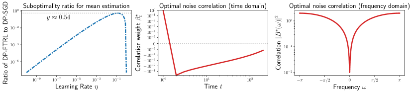
Figure 1: Left: The ratio of the asymptotic suboptimalities of DP-FTRL to DP-SGD for mean estimation vs. the learning rate $\eta$. DP-FTRL is never worse but is orders of magnitude better at $\eta\to 0$ or $\eta\to 1$. Middle & Right: Time- and frequency-domain descriptions of the optimal noise correlations for mean estimation (defined in Theorem 2.1).

Consider a distribution $\mathbb{P}_{\sf{data}}$ with $|z-\mathbb{E}[z]|\leq\sigma_{\sf{sgd}}$ and $|z|\leq 1$ a.s. for $z\sim\mathbb{P}_{\sf{data}}$. Our objective now is

$$\textstyle F\left({\theta}\right)=\frac{1}{2}\,\mathbb{E}_{z\sim\mathbb{P}_{\sf{data}}}{(\theta-z)^{2}}\quad\text{with}\quad f\left({\theta;z}\right)=\frac{z^{2}}{2}-z\theta,\quad\text{and}\quad r\left({\theta}\right)=\frac{\theta^{2}}{2}\,.$$ (6)

We show a strict separation between DP-FTRL and DP-SGD for this simple minimization problem.

Theorem 2.1.

Consider the setting above with learning rate $\eta\leq 1$ and clip norm $G=1$. Then, the asymptotic suboptimality of a $\rho$-zCDP sequence $(\theta_{t})_{t=0}^{\infty}$ obtained via DP-SGD is $F_{\infty}({\bm{\beta}}_{\sf{dpsgd}})=\Theta(\eta\rho^{-1}+\eta\sigma_{\sf{sgd}}^{2})$. Further, the asymptotic suboptimality of any $\rho$-zCDP sequence $(\theta_{t})_{t=0}^{\infty}$ from DP-FTRL is

$${}\inf_{\bm{\beta}}F_{\infty}({\bm{\beta}})=F_{\infty}({\bm{\beta}}^{\star})=\Theta\left(\eta^{2}\rho^{-1}\log^{2}(1/\eta)+\eta\sigma_{\sf{sgd}}^{2}\right)\,.$$

The infimum above is attained by $\beta^{\star}_{t}=(-1)^{t}{1/2\choose t}(1-\eta)^{t}$, where ${1/2\choose t}=\prod_{k=0}^{t-1}\frac{1/2-k}{t-k}$.

Proof Sketch.

Using tools from frequency domain analysis of linear time invariant systems Oppenheim et al. (1997), we can show that the asymptotic variance $\mathbb{E}(\theta_{t}-\mathbb{E}[z])^{2}$ is an integral of $|B(\omega)|^{2}$. The sensitivity is an integral of $|B(\omega)|^{-2}$ (cf. (5)) so that $F_{\infty}$ is a product of these integrals. Its minimizer $B^{\star}$ can be analytically computed in the Fourier domain (Figure 1, right). An inverse Fourier transform yields the claimed expression for ${\bm{\beta}}^{\star}$ (Figure 1, center). ∎

The optimal $\rho^{-1}$ coefficient is $\eta^{2}\log^{2}(1/\eta)$, which is an improvement over DP-SGD’s $\eta$ (Figure 1, left).

$\nu$-DP-FTRL/$\nu$-Noisy-FTRL: Theorem 2.1 gives an analytical expression for the optimal noise correlation weights for DP-FTRL for this simplified setting. We parameterize it with a parameter $0<\nu<1$ to define

$$\textstyle\hat{\beta}_{t}^{\nu}:=(-1)^{t}{1/2\choose t}(1-\nu)^{t}\,.$$ (7)

We analyze this choice theoretically for the setting of Noisy-FTRL and demonstrate near optimality. Later, for our experiments with DP-FTRL, we tune $\nu$ as a hyperparameter to tune. We call this approach (with clipping) $\nu$-DP-FTRL and (without clipping) $\nu$-Noisy-FTRL.

2.2 Asymptotic Suboptimality for Linear Regression

We now give a precise analysis of $F_{\infty}$ for linear regression with $\nu$-Noisy-FTRL.We will use this to derive non-asymptotic privacy-utility bounds for DP-FTRL at the end of this section.

We consider (unregularized) linear regression with loss function $f\left({\bm{\theta};\left({{\bm{x}},y}\right)}\right)=\frac{1}{2}\left({y-\left\langle{\bm{\theta}},{{\bm{x}}}\right\rangle}\right)^{2}$ so that

$$\textstyle F(\bm{\theta})=\frac{1}{2}\,\,\mathbb{E}_{({\bm{x}},y)\sim\mathbb{P}_{\sf{data}}}\left(y-\langle\bm{\theta},{\bm{x}}\rangle\right)^{2}\,.$$ (8)

We assume $d$-dimensional Gaussian covariates ${\bm{x}}\sim\mathcal{N}(\bm{0},{\bm{H}})$ and independent Gaussian residuals $y-\langle\bm{\theta}_{\star},{\bm{x}}\rangle\sim\mathcal{N}(0,\sigma_{\sf{sgd}}^{2})$ where $\bm{\theta}_{\star}=\operatorname*{arg\,min}F$. We make these assumptions for ease of presentation; we state and prove our results under weaker assumptions in the supplement. Further, we assume that $F$ is $L$-smooth and $\mu$-strongly convex (equivalently, $\mu{\bm{I}}\preceq{\bm{H}}\preceq L{\bm{I}}$ since the input covariance ${\bm{H}}$ is also the Hessian of $F$).

We express the bounds on $F_{\infty}$ in terms of the correlation weights ${\bm{\beta}}$ and the problem parameters $\rho,G$ which, for DP-FTRL, denote the target privacy level and the gradient clip norm respectively. See §C for proofs.

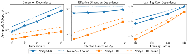
Figure 2: Linear regression simulations: We plot the empirically observed asymptotic suboptimality of $\nu$-Noisy-FTRL/Noisy-SGD and their theoretical bounds with $d=128$ (varied in the left plot) where the Hessian ${\bm{H}}$ has eigenvalues $\lambda_{k}=1/k$ (varied as $k^{-\alpha}$ for $\alpha\in[0.4,1]$ in the middle plot), and learning rate $\eta=0.02$ (varied in the right plot). The slope of the corresponding empirical and theoretical lines are nearly equal, showing the tightness of the theory. In particular, we observe that Noisy-SGD has a linear dependence on the dimension (slope $1.00$) and is nearly constant w.r.t. the effective dimension (slope $0.18$) while Noisy-FTRL has a near-linear dependence on the effective dimension (slope $0.94$). Noisy-FTRL (slope $2.03$) also has a better dependence on the learning rate than Noisy-SGD (slope $1.27$).

Theorem 2.2.

Let $c,C_{1},C_{2}$ denote universal constants. For $\eta\leq c/{\sf Tr}\left[{\bm{H}}\right]$, we have

(Noisy-SGD) $$F_{\infty}({\bm{\beta}}^{\sf{sgd}})=\Theta\left(\eta dG^{2}{\rho^{-1}}+\eta\sigma_{\sf{sgd}}^{2}{\sf Tr}\left[{\bm{H}}\right]\right) \quad\text{ with }{\bm{\beta}}^{\sf{sgd}}=(1,0,\ldots)\,,$$

($$\nu F_{\infty}(\hat{{\bm{\beta}}^{\nu}})\leq C_{1}\left(\eta^{2}G^{2}\rho^{-1}\log^{2}\tfrac{1}{\nu}+\eta\sigma_{\sf{sgd}}^{2}\right){\sf Tr}\left[{\bm{H}}\right] \quad\text{ with }\nu\leq\eta\mu,\text{ and}$$-Noisy-FTRL)

(Lower bound) $$F_{\infty}({\bm{\beta}})\geq C_{2}\left(\eta^{2}G^{2}{\rho^{-1}}+\eta\sigma_{\sf{sgd}}^{2}\right){\sf Tr}\left[{\bm{H}}\right] \quad\text{ for all }{\bm{\beta}}\text{ with }{\left\|{{\bm{\beta}}}\right\|}_{1}<\infty\,.$$

This shows the near-optimality of $\nu$-Noisy-FTRL and a provable gap between Noisy-FTRL and Noisy-SGD, as we discuss below. Observe that our bounds separate the contributions arising from correlated noise ($\rho^{-1}$ term) and those from the inherent noise in the linear model ($\sigma_{\sf{sgd}}^{2}$ term). We focus on the effect of correlation because the effect of latter noise is the same across all choices of ${\bm{\beta}}$. We plot the differences in Figure 2.

Exponential separation between Noisy-SGD and Noisy-FTRL: Noisy-SGD’s stationary error depends on the ambient dimension $d$, while the lower bound depends on the effective dimension $d_{\sf eff}={\sf Tr}\left[{\bm{H}}\right]/{\left\|{{\bm{H}}}\right\|}_{2}$ of the covariance ${\bm{H}}$. We have, $d_{\sf eff}\leq d$ with equality when all the eigenvalues of ${\bm{H}}$ are equal but $d_{\sf eff}\ll d$ when the eigenvalues of ${\bm{H}}$ decay rapidly or it is nearly low rank. This is true particularly for overparameterized models where the features may be highly correlated resulting in an approximately low-rank covariance.

For instance, if the eigenvalues of ${\bm{H}}$ are $(1,1/d,\ldots,1/d)$, then $d_{\sf eff}\leq 2$. Then, Noisy-FTRL’s error of $O(\eta^{2}\rho^{-1}\log^{2}(d/\eta))$ is exponentially better than Noisy-SGD’s $\Theta(\eta\rho^{-1}d)$. The learning rate dependence of Noisy-SGD is also suboptimal, similar to §2.1. This result is also confirmed empirically in Figure 2 (right).

Table 2: Comparison to prior work: We apply our theory to compute $F_{\infty}$ for linear regression given choices of ${\bm{B}}$ used in prior work. Though certain choices of the noise correlation ${\bm{\beta}}$ may be optimal for finite linear counting queries Fichtenberger et al. (2023), our results show that they have $F_{\infty}=\infty$ because the sensitivity diverges as $T\to\infty$. $\nu$-Noisy-FTRL effectively introduces an additional damping term $(1-\nu)^{t}$ in the correlations of Fichtenberger et al. (2023) to achieve near-optimality for linear regression. Damping similarly helps for anti-PGD Orvieto et al. (2022), where the resulting error is the geometric mean of the lower bound and the bound of Noisy-SGD from Theorem 2.2.

Algorithm Noise Correlation Weights ${\bm{\beta}}$ Sensitivity in $T$ steps $\gamma_{T}({\bm{\beta}})^{2}$ Asymptotic Suboptimality $F_{\infty}({\bm{\beta}})$ Fichtenberger et al. (2023) Eq. (7) with $\nu=0$ $\log T$ $\infty$ $\nu$-Noisy-FTRL (Ours) Eq. (7) with $0<\nu\leq\eta\mu$ $\log(1/\nu)$ $\eta^{2}G^{2}\rho^{-1}{\sf Tr}\left[{\bm{H}}\right]\log^{2}(1/\nu)$ Anti-PGD Orvieto et al. (2022) $(1,-1,0,\ldots)$ $T$ $\infty$ Anti-PGD + Damping $(1,-(1-\nu),0,\ldots)$ $1/\nu$ $\eta^{3/2}G^{2}\rho^{-1}\sqrt{d{\sf Tr}\left[{\bm{H}}\right]}$

2.3 Finite-time Privacy-Utility Bounds for Linear Regression

Noisy-FTRL, which we analyzed so far, is not differentially private. Differential privacy requires gradient clipping that significantly complicates the analysis. However, for a finite time horizon $T$, we can argue using concentration that $\nabla f\left({\bm{\theta};{\bm{z}}}\right)$ is bounded with high probability and clipping can be avoided. Formal statements and proofs for the finite-time analysis are given in Appendix D.

Consider DP-FTRL with noise correlation $\hat{}{\bm{\beta}}^{\nu}$ from (7) with $\nu=\eta\mu$ and gradients clipped to any $\ell_{2}$-norm $G$. As mentioned in §1.1, the outputs $(\bm{\theta}_{1},\ldots,\bm{\theta}_{T})$ of DP-FTRL are $\rho$-zCDP. For an appropriate choice of $\eta$, we give utility bounds in terms of the effective dimension $d_{\sf eff}$ and the condition number $\kappa=L/\mu$:

1. For $\eta$ small enough, we have with probability at least $1-p$ that

   $${}\max_{t<T}{\left\|{{\bm{g}}_{t}}\right\|}_{2}\leq c\max\left\{{\sf Tr}\left[{\bm{H}}\right]{\left\|{\bm{\theta}_{0}-\bm{\theta}_{\star}}\right\|}_{2},\sigma_{\sf{sgd}}\sqrt{{\sf Tr}\left[{\bm{H}}\right]}\right\}{\rm polylog}\left(T/p\right)=:G\,.$$ (9)

   Let $\mathcal{E}$ denote this event. If it holds, no gradients are clipped and DP-FTRL coincides with Noisy-FTRL.

2. For $T\geq\widetilde{\Omega}(\kappa^{2}d_{\sf eff}^{2}d/\rho)$, we have (omitting log factors and $o(1/T^{2})$ terms and taking ${\left\|{{\bm{H}}}\right\|}_{2}=1$):

   $${}\mathbb{E}\left[(F(\bm{\theta}_{t})-F(\bm{\theta}_{\star}))\cdot\mathbbm{1}\left(\mathcal{E}\right)\right]\lesssim\begin{cases}\kappa\,d_{\sf eff}\left(\frac{dd_{\sf eff}{\left\|{\bm{\theta}_{0}-\bm{\theta}_{\star}}\right\|}_{2}^{2}}{\rho T}+\frac{d\sigma_{\sf{sgd}}^{2}}{\rho T}+\frac{\sigma_{\sf{sgd}}^{2}}{T}\right)&\text{ for DP-SGD},\\ \kappa d_{\sf eff}\left(\frac{\kappa d_{\sf eff}^{2}{\left\|{\bm{\theta}_{0}-\bm{\theta}_{\star}}\right\|}_{2}^{2}}{\rho T^{2}}+\frac{\kappa d_{\sf eff}\sigma_{\sf{sgd}}^{2}}{\rho T^{2}}+\frac{\sigma_{\sf{sgd}}^{2}}{T}\right)&\text{ for $\nu$-DP-FTRL}.\end{cases}$$

Thus, the dimension $d$ in DP-SGD’s bound effectively becomes $\kappa d_{\sf eff}/T$ for DP-FTRL, leading to a better dimension dependence. While faster $1/(\rho T^{2})$ rates are known for DP-SGD-style algorithms for linear regression Varshney et al. (2022); Liu et al. (2023), such algorithms require sophisticated adaptive clipping strategies. Our algorithms use a fixed clipping norm $G$ and a fixed noise multiplier $\sigma_{\sf{dp}}$ independent of $T$; the bounds presented above are, to the best of our knowledge, the best known in the literature for DP-SGD in this setting. We leave the exploration of combining adaptive clipping with correlated noise for future work.

3 Asymptotic Suboptimality for General Strongly Convex Functions

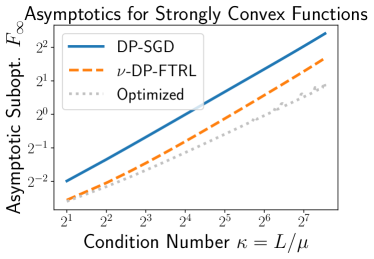
Figure 3: DP-FTRL attains a tighter bound on $F_{\infty}$ with the growing condition number. Here, “Optimized” approximately minimizes (10). The plots holds for smooth and strongly convex functions ($L=1=G,\sigma_{\sf{sgd}}=0$).

We now generalize §2.2 to general strongly convex problems. Here, we bound the asymptotic suboptimality of DP-FTRL and DP-SGD by the value of a convex program.

Theorem 3.1.

Suppose $f(\,\cdot\,;{\bm{z}})$ is $G$-Lipschitz, and the stochastic gradients are uniformly bounded as ${\left\|{\nabla_{\theta}f\left({\bm{\theta};{\bm{z}}}\right)-\mathbb{E}_{{\bm{z}}^{\prime}\sim\mathbb{P}_{\sf{data}}}\left[{\nabla_{\theta}f\left({\bm{\theta};{\bm{z}}^{\prime}}\right)}\right]}\right\|}_{2}\leq\sigma_{\sf{sgd}}$. Then, if $F$ is $\mu$-strongly convex and $L$-smooth, we can bound $F_{\infty}$ for any noise correlation $B\left({\omega}\right)$ in the frequency domain as:

$$\min_{\begin{subarray}{c}{\psi}:[-\pi,\pi]\to\mathbb{R}_{+}\\ {\psi}\in\mathcal{C}\left({\eta,L,\mu}\right)\end{subarray}}\frac{Ld}{2\pi}\int_{-\pi}^{\pi}\left({{G^{2}}{\rho^{-1}}|B\left({\omega}\right)|^{2}\gamma_{\infty}(B)^{2}+\sigma_{\sf{sgd}}^{2}}\right){\psi}(\omega)\,{\mathrm{d}}\omega\,,$$ (10)

where $\gamma_{\infty}(B)$ is the limiting sensitivity from Eq. (5), and $\mathcal{C}\left({\eta,\mu,L}\right)$ is a convex set (details in Appendix E).

While technically an infinite dimensional optimization problem over the function ${\psi}$, we can approximate the solution by discretizing ${\psi}$ into $k$ points uniformly over $[-\pi,\pi]$. Further, if we discretize $B$ similarly, we can obtain a second-order cone program with $k$ conic constraints and $O(k)$ decision variables. As $k\to\infty$, the solution approaches the solution to (10). Empirically, we observe that the values stabilize quickly as $k$ increases. We stop the computation when the change in bound as a function of $k$ drops below a threshold. We use $k=1000$ for Figure 3.

Further, given the optimal ${\psi}={\psi}^{\star}$, we can run an alternating minimization where we minimize the objective of (10) with respect to ${\psi}$ for fixed $B$ and with respect to $B$ for fixed ${\psi}$. This leads to an iteratively improving choice of $B$. We find empirically that this iterative procedure converges quickly and leads to a provable theoretical gap between the upper bounds on $F_{\infty}$ achievable by DP-SGD and DP-FTRL.

We numerically compare the bound (10) for DP-SGD and $\nu$-DP-FTRL with weights from (7). Figure 3 shows that the gap between DP-SGD and $\nu$-DP-FTRL is multiplicative, i.e., the absolute gap grows with the increasing condition number $\kappa=L/\mu$ (which reflects practical scenarios). The suboptimality of “Optimized” DP-FTRL (optimized as described above) grows even more slowly with $\kappa$.

Overall, $\nu$-DP-FTRL significantly improves upon DP-SGD and has only a single tunable parameter $\nu$ and no expensive computation to generate the noise correlations. We focus on $\nu$-DP-FTRL for experiments in this paper, but leave the possibility of improving results further based on Optimized DP-FTRL for future work.

4 Experiments

DP-FTRL Variant Citation Corr. matrix ${\bm{B}}$ Anytime? Computation Cost Generation Training (per step) DP-SGD Abadi et al. (2016) Identity ✓ $O\left({1}\right)$ $O\left({1}\right)$ Honaker/TreeAgg Kairouz et al. (2021a) Lower-Triangular (LT) ✓ $O\left({1}\right)$ $O\left({\log T}\right)$ Optimal CC Fichtenberger et al. (2023) Toeplitz & LT ✓ $O\left({1}\right)$ $O(T)$ $\nu$-DP-FTRL Ours Toeplitz & LT ✓ $O(1)$ $O(T)$ FFT Choquette-Choo et al. (2023b) Toeplitz - $O(1)$ $O\left({T\log^{2}T}\right)$ Full Honaker Honaker (2015) Arbitrary - $O(T^{2})$ $O(T^{2})$ Multi-Epoch (ME) Choquette-Choo et al. (2023b) Arbitrary - $O\left({T^{3}}\right)$ $O\left({T^{2}}\right)$

Table 3: Variants of DP-FTRL: the noise correlation matrix ${\bm{B}}$ and whether the correlation matrix ${\bm{B}}$ can be created/optimized agnostic to the time horizon $T$ (denoted as “Anytime”), and the computation cost.

We demonstrate the practical benefits of $\nu$-DP-FTRL for deep learning tasks. This approach has a single tunable parameter $\nu$ that can easily be tuned based on minimizing the squared error (3) as in prior work.

Comparing Computation (Table 3): While optimized matrices (e.g. “ME” in Table 3) have the state-of-the-art privacy-utility tradeoffs in private learning (without amplification), their computational cost scales as $O(T^{3})$. For example, generating the correlation matrix ${\bm{B}}$ for $T=10^{4}$ takes around $24$ hours Choquette-Choo et al. (2023b). Moreover, it has a $O(T^{2})$ cost per-step. We find in this section that $\nu$-DP-FTRL achieves near state-of-the-art privacy-utility tradeoffs at a much smaller computational cost of $O(T)$ per iteration.

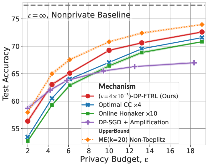
(a) Example-level DP on CIFAR-10 (image classification).

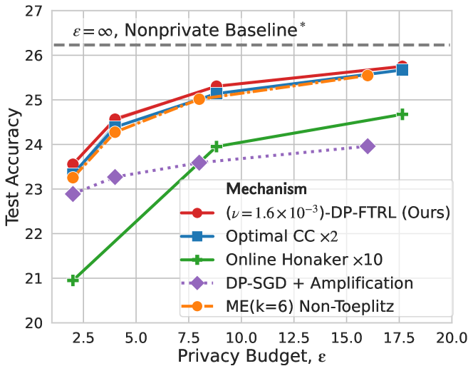
(b) User-level DP on StackOverflow (language modeling).

Figure 4: The proposed $\nu$-DP-FTRL outperforms all other efficient and anytime mechanisms. It also nearly equal or slightly outperform the state-of-the-art “ME” mechanism that requires significantly more compute (cf. Table 3). ^∗The nonprivate baseline for StackOverflow uses per-user clipping as we found this improves performance by $\approx 0.5\%$-points and improves training stability.

We compare with other anytime approaches for which the matrices ${\bm{B}}$ can extended to any time horizon $T$. The practitioner then need not specify $T$ in advance, but rather, can train for as long as necessary to achieve minimal model loss—it is common to, e.g., let algorithms run until certain conditions, like a maximum difference on the train-test loss, are met Morgan & Bourlard (1989). Moreover, general matrices ${\bm{B}}$ become prohibitive in terms of compute/memory as models scale up Kaplan et al. (2020); Anil et al. (2023).

Experiment Setup: We use two standard benchmarks: example-level DP for image classification on the CIFAR-10 dataset and user-level DP for language modeling on the StackOverflow dataset. We use the exact same setup as Kairouz et al. (2021a). We also stamp/restart all baselines as suggested in Choquette-Choo et al. (2023b). This gives the baselines an advantage of an additional tuning parameter (tuned to minimize the squared error (3)), but does not affect their per-step training cost. We denote this by the suffix “$\times S$” for $S>1$ in the plot. We tune all CIFAR-10 hyperparameters with a grid search, while we use hyperparameters reported from previous works for StackOverflow. Appendix G gives the full setup.

Main Results: Across both datasets, $\nu$-DP-FTRL outperforms all existing anytime mechanisms by a significant margin (Figure 4(a)). We find an average $3$pp improvement that grows as $\varepsilon$ becomes small. Indeed, the proposed $\nu$-DP-FTRL makes up 30-80% of the gap between previous efficient approaches and the state-of-the-art and computationally intense ME approach. For instance, at $\varepsilon=10$, we have $\nu$-DP-FTRL at $69.26\%$ nearly matches ME at $70.83\%$. For StackOverflow, we find that $\nu$-DP-FTRL outperforms the state-of-the-art ME across all $\varepsilon$ (Figure 4(b)) by $\approx 0.3\%$-points while requiring significantly less computation.

As $\varepsilon$ becomes small, DP-SGD can outperform DP-FTRL due to privacy amplification. We find that $\nu$-DP-FTRL outperforms DP-SGD for $\varepsilon\geq 4$ on CIFAR-10 ($63.02\%$ vs. $62.02\%$) and around $\varepsilon\approx 2$ for StackOverflow ($23.6\%$ versus $22.6\%$), showing its broad applicability. Finally, we observe that that our mechanism achieves near non-private baselines on StackOverflow. A model trained via $\nu$-DP-FTRL gets $25.3\%$ validation accuracy at $\varepsilon=8$, a mere $1\%$-point off from the nonprivate baseline.

5 Conclusion

This work shows a clear separation between the noisy training dynamics with uncorrelated (DP-SGD) and correlated noise (DP-FTRL) for linear regression. The matching upper/lower bounds reveal that DP-FTRL has a better dependence than DP-SGD on problem parameters such as the effective dimension and condition number. Inspired by the theory, we propose $\nu$-DP-FTRL and validated its empirical performance on two DP tasks spanning image and language modalities. We found it can compete the state-of-the-art while circumventing the need for any expensive computations like the semi-definite programs used in prior work. This work opens up several exciting directions including leveraging correlated-noise mechanisms for instance-optimal bounds and further improving the computational efficiency to enable large-scale private training.

Acknowledgements

The authors thank H. Brendan McMahan, Fabian Pedregosa, Ian R. Manchester, Keith Rush, and Rahul Kidambi for fruitful discussions and helpful comments.

Appendix

Appendix A Further Background on DP-FTRL

In this appendix, we give a more detailed background of DP-FTRL, and its exact notion of DP.

A.1 DP-FTRL: The Matrix Mechanism for Private Learning

The DP-FTRL algorithm Kairouz et al. (2021a); Denisov et al. (2022) is obtained by adapting the matrix mechanism, originally designed for linear counting queries Li et al. (2015), to optimization with a sequence $({\bm{g}}_{0},\ldots,{\bm{g}}_{T-1})$ of gradient vectors.

Algorithm 1 gives a detailed description of DP-FTRL. We given an alternate description of DP-FTRL with an invertible lower-triangular noise correlation matrix ${\bm{B}}\in\mathbb{R}^{T\times T}$. Denoting ${\bm{C}}={\bm{B}}^{-1}$, the iterates of DP-FTRL are generated by the update

$$\begin{pmatrix}\bm{\theta}_{1}\\ \vdots\\ \bm{\theta}_{T}\end{pmatrix}=\begin{pmatrix}\bm{\theta}_{0}\\ \vdots\\ \bm{\theta}_{T-1}\end{pmatrix}-\eta{\bm{B}}\left({{\bm{C}}\begin{pmatrix}{\bm{g}}_{0}\\ \vdots\\ {\bm{g}}_{T-1}\end{pmatrix}+\begin{pmatrix}{\bm{w}}_{0}\\ \vdots\\ {\bm{w}}_{T-1}\end{pmatrix}}\right)$$ (11)

where $\eta$ is a learning rate and ${\bm{w}}_{t}\sim\mathcal{N}(\bm{0},G^{2}\sigma_{\sf{dp}}^{2}{\bm{I}}_{d})$ is i.i.d. Gaussian noise with a noise multiplier $\sigma_{\sf{dp}}$ and $G$ is the $\ell_{2}$ clip norm. It is common to refer to ${\bm{C}}$ as the encoder, while ${\bm{B}}$ is referred to as the decoder.

This privacy of (11) can be seen a postprocessing of a single application of the Gaussian mechanism. Let ${\bm{G}},{\bm{W}}\in\mathbb{R}^{T\times d}$ denote the matrix where each row is the gradient ${\bm{g}}_{t}$ (and respectively the noise ${\bm{w}}_{t}$). Then, (11) is effectively the postprocessing of one run of the Gaussian mechanism ${\bm{C}}{\bm{G}}+{\bm{W}}$. Under a neighborhood model that can change one row of ${\bm{G}}$, it can be seen that the maximum sensitivity of this operation is $\max_{t}\|{\bm{C}}_{:,t}\|_{2}^{2}$ Denisov et al. (2022). This sensitivity logic also holds for adaptively chosen gradients; we postpone a formal description to Section A.2.

Connection to the exposition in prior work: Prior work introduced DP-FTRL differently. Letting ${\bm{A}}\in\mathbb{R}^{T\times T}$ denote the lower triangular matrix of all ones, update (11) can also be written as

$$\begin{pmatrix}\bm{\theta}_{1}-\bm{\theta}_{0}\\ \vdots\\ \bm{\theta}_{T}-\bm{\theta}_{0}\end{pmatrix}=-\eta\widetilde{\bm{B}}\left({{\bm{C}}\begin{pmatrix}{\bm{g}}_{0}\\ \vdots\\ {\bm{g}}_{T-1}\end{pmatrix}+\begin{pmatrix}{\bm{w}}_{0}\\ \vdots\\ {\bm{w}}_{T-1}\end{pmatrix}}\right)\,,$$ (12)

where $\widetilde{\bm{B}}={\bm{A}}{\bm{B}}$. The equivalence between (11) and (12) can be seen by multiplying (11) by ${\bm{A}}$, which is also equivalent to taking the cumulative sum of the rows of a matrix. In this notation, the objective from (3) used in previous work to find the matrix ${\bm{B}}$ can equivalently be written as

$$\varphi({\bm{B}})=\|\widetilde{\bm{B}}\|_{F}^{2}=\|{\bm{A}}{\bm{B}}\|_{F}^{2}\,.$$

DP-FTRL with Toeplitz matrices: We focus on the class of lower-triangular and Toeplitz matrices ${\bm{B}}$. That is, $[{\bm{B}}]_{t,t^{\prime}}=\beta_{t-t^{\prime}}$ for all $t\geq t^{\prime}$ where ${\bm{\beta}}=(\beta_{0},\ldots,\beta_{T-1})$ is the first column of ${\bm{B}}$. In this case, (11) reduces to this simple update:

$$\bm{\theta}_{t+1}=\bm{\theta}_{t}-\eta\left({\bm{g}}_{t}+\sum_{\tau=0}^{t}\beta_{\tau}{\bm{w}}_{t-\tau}\right)\,.$$ (13)

This lets us study DP-FTRL as a time-invariant stochastic process and characterize its stationary behavior.

A.2 Differential Privacy in Adaptive Streams

Neighboring streams: We consider learning algorithms as operating over streams of gradients ${\bm{g}}_{0},{\bm{g}}_{1},\ldots\in\mathbb{R}^{d}$. We consider differential privacy (DP) under the “zero-out” notion of neighborhood Kairouz et al. (2021a). Two streams ${\bm{G}}=({\bm{g}}_{0},\ldots,{\bm{g}}_{T-1})$ and ${\bm{G}}^{\prime}=({\bm{g}}_{0}^{\prime},\ldots,{\bm{g}}_{T-1}^{\prime})$ of length $T$ are said to be neighbors if ${\bm{g}}_{\tau}={\bm{g}}_{\tau}^{\prime}$ for all positions $\tau\leq T-1$ except possibly one position $t$ where one of ${\bm{g}}$ or ${\bm{g}}^{\prime}$ is the zero vector.

DP with adaptive continual release: It is customary to formalize DP with adaptive streams as a privacy game between a mechanism $\mathcal{M}$ and a privacy adversary $\mathcal{A}$. This is known as the adaptive continual release setting Jain et al. (2023). The game makes a binary choice $b\in\{0,1\}$ ahead of time — this remains fixed throughout and is not revealed to either $\mathcal{M}$ or $\mathcal{A}$. Each round $t$ consists of four steps:

• $\mathcal{M}$ sends the current model parameters $\bm{\theta}_{t}$ to the adversary $\mathcal{A}$;

• $\mathcal{A}$ generates two gradient vectors ${\bm{g}}_{t},{\bm{g}}_{t}^{\prime}$ (e.g. as $\nabla f(\bm{\theta}_{t};{\bm{z}}_{t})$ for ${\bm{z}}_{t}\sim\mathbb{P}_{\sf{data}}$ or simply the zero vector);

• the game accepts these inputs if the partial streams $({\bm{g}}_{0},\ldots,{\bm{g}}_{t})$ and $({\bm{g}}_{0}^{\prime},\ldots,{\bm{g}}_{t}^{\prime})$ are neighbors;

• $\mathcal{M}$ receives ${\bm{g}}_{t}$ if $b=0$ else ${\bm{g}}_{t}^{\prime}$.

DP in this setting requires that the adversary cannot infer the value of $b$, i.e., the distribution of $\bm{\theta}_{0:T}|b=0$ to be “close” to that of $\bm{\theta}_{0:T}|b=1$ (where the definition of “closeness” depends on the DP variant). For instance, $(\varepsilon,\delta)$-DP Dwork et al. (2006) requires for each $b\in\{0,1\}$ and any outcome set $S$ that

$$\mathbb{P}(\bm{\theta}_{0:T}\in S\,|\,b)\leq\exp(\varepsilon)\,\mathbb{P}(\bm{\theta}_{0:T}\in S\,|\,1-b)+\delta\,.$$

Similarly, $\rho$-zCDP Bun & Steinke (2016) in this setting requires that the Rényi $\alpha$-divergence between the distribution $P_{0}$ of $\bm{\theta}_{0:T}|b=0$ and the distribution $P_{1}$ of $\bm{\theta}_{0:T}|b=1$ are close:

$$D_{\alpha}(P_{0}\|P_{1})\leq\rho\alpha$$

for all $\alpha\in(0,\infty)$. Following standard arguments (e.g. Balle et al., 2020), $\rho$-zCDP in this setting implies $(\varepsilon_{\delta},\delta)$-DP with

$$\varepsilon_{\delta}\leq\inf_{\alpha>1}\left\{\rho\alpha+\frac{1}{\alpha-1}\log\left(\frac{1}{\alpha\delta}\right)+\log(1-\alpha^{-1})\,.\right\}$$

DP-FTRL satisfies a zCDP guarantee as described in Theorem 1.1 in §1. This guarantee is equivalent to the one obtained by interpreting (11) as the postprocessing of one run one run of the Gaussian mechanism ${\bm{C}}{\bm{G}}+{\bm{W}}$.

Appendix B Asymptotics of DP-FTRL for Mean Estimation

We now prove Theorem 2.1 on mean estimation.

Proof of Theorem 2.1.

Since $|\nabla f(\theta;z)|=|z|\leq 1$ and $G\geq 1$, there is no gradient clipping. Setting $\delta_{t}=\theta_{t}-\mathbb{E}[z]$ and $w_{\sf{sgd}}=(z-\mathbb{E}[z])/\sigma_{\sf{sgd}}$, the updates (2) can be written:

$$\delta_{t+1}=(1-\eta)\delta_{t}+\eta\sigma_{\sf{sgd}}w_{\sf{sgd}}-\eta\sigma_{\sf{dp}}G\sum_{\tau=0}^{t}\beta_{\tau}w_{t-\tau}\,.$$

We can then use the results from §F.1 (Theorem F.2 in particular) to obtain an expression for the steady state error:

$$F_{\infty}(B)=\frac{\eta^{2}}{2\pi}\int_{-\pi}^{\pi}\frac{|B\left({\omega}\right)|^{2}G^{2}\sigma_{\sf{dp}}^{2}\gamma_{\infty}\left({B}\right)^{2}+\sigma_{\sf{sgd}}^{2}}{|1-\eta-\exp\left({i\omega}\right)|^{2}}\,{\mathrm{d}}\omega\,.$$

Here, we used the fact that the SGD noise $z-\mathbb{E}\left[{z}\right]$ is i.i.d. in each step and independent of the DP noise ${\bm{w}}$, so that the power spectral density of the sum of these two noise sources is simply the sum of the power spectral densities of the individual sources, with the power spectral density of the SGD noise being constant and equal to $\sigma_{\sf{sgd}}$.

Thus $F_{\infty}$ is a product of a linear function of $|B|^{2}$ and $\frac{1}{|B|^{2}}$ (the latter through $\gamma_{\infty}\left({B}\right)$ via (5)). By the Cauchy-Schwarz inequality, the product is minimized when

$$\frac{|B\left({\omega}\right)|^{2}}{|1-\eta-\exp\left({i\omega}\right)|^{2}}=\frac{1}{|B\left({\omega}\right)|^{2}}\implies|B^{\star}\left({\omega}\right)|=|\sqrt{1-\eta-\exp\left({i\omega}\right)}|\,.$$ (14)

The proof of the error bound now follows by computing and bounding standard integrals (in particular, see §F.4 and F.15 for the elliptic integrals coming from the $\sigma_{\sf{dp}}^{2}$ term and C.5 for the $\sigma_{\sf{sgd}}^{2}$ term).

Next, we derive the time-domain description. For this, we take $B^{\star}(\omega)=\sqrt{1-(1-\eta)\exp(-i\omega)}$ (which amounts to fixing a phase in (14) above). We use the Maclaurin series expansion $\sqrt{1+z}={1/2\choose t}z^{t}$ of the square root function to get

$$B^{\star}(\omega)=\sum_{t=0}^{\infty}(-1)^{t}{1/2\choose t}(1-\eta)^{t}\exp(-i\omega t)\,.$$

Comparing this to the definition of the discrete-time Fourier transform $B^{\star}(\omega)=\sum_{t=0}^{\infty}\beta^{\star}_{t}\exp(-i\omega t)$ gives the claimed expression for ${\bm{\beta}}^{\star}$. ∎

Appendix C Asymptotics of DP-FTRL for Linear Regression

The goal of this section is to prove Theorem 2.2. The proof relies heavily on the following matching upper and lower bounds on the stationary error of Noisy-FTRL with any noise correlations ${\bm{\beta}}$ in the frequency domain using its discrete-time Fourier transform (DTFT) $B$ as:

$$F_{\infty}(B) =\Theta\left(\eta\sigma_{\sf{sgd}}^{2}{\sf Tr}\left[{\bm{H}}\right]+\eta^{2}G^{2}\rho^{-1}\gamma_{\infty}(B)^{2}\int_{-\pi}^{\pi}|B(\omega)|^{2}h(\omega)\,{\mathrm{d}}\omega\right)\,,$$ (15)

where the function $h:[-\pi,\pi]\to\mathbb{R}$ depends on the eigenvalues $\lambda_{1},\ldots,\lambda_{d}$ of the input covariance ${\bm{H}}$:

$$h(\omega)=\sum_{j=1}^{d}\frac{\lambda_{j}}{|1-\exp(i\omega)-\eta\lambda_{j}|^{2}}\,.$$ (16)

The outline of the section is

• Section C.1: Setup, including notation, and assumptions.

• Section C.2: Proofs of the upper bound of (15), specifically Theorem C.15 (see also Theorem C.14 for the time-domain description).

• Section C.3: Proofs of the lower bound of (15), specifically Theorem C.17.

• Section C.4: Asymptotics of $\nu$-Noisy-FTRL.

• Section C.5: Asymptotics of anti-PGD (see Table 2).

• Section C.6: Proofs of intermediate technical results.

The separation between Noisy-SGD and $\nu$-Noisy-FTRL is further illustrated in Table 4. Following common practice (e.g. Caponnetto & De Vito, 2007), we compare the rates for various regimes of eigenvalue decays for ${\bm{H}}$.

Table 4: Asymptotic suboptimality of Noisy-SGD and Noisy-FTRL for linear regression with Gaussian inputs based on the eigenvalues $\lambda_{k}$ of the Hessian ${\bm{H}}$. We give the bounds in terms of the learning rate $\eta$, dimension $d$, the effective dimension $d_{\sf eff}={\sf Tr}\left[{\bm{H}}\right]/{\left\|{{\bm{H}}}\right\|}_{2}$, and the noise variance $\rho^{-1}$ representing the privacy level. We take $G=1$ and ${\left\|{{\bm{H}}}\right\|}_{2}=1$ w.l.o.g. Noisy-FTRL is always better at large dimension $d$ or small learning rate $\eta$.

Eigenvalues of ${\bm{H}}$ Effective dim. $d_{\sf eff}$ Noisy-SGD Noisy-FTRL Ratio of $\frac{\text{Noisy-FTRL}}{\text{Noisy-SGD}}$ $\lambda_{k}=1$ $d$ $\eta d\rho^{-1}$ $\eta^{2}d\rho^{-1}\log^{2}(\frac{1}{\eta})$ $\eta\log^{2}(\frac{1}{\eta})$ $\lambda_{k}=1/\sqrt{k}$ $\sqrt{d}$ $\eta d\rho^{-1}$ $\eta^{2}\sqrt{d}\rho^{-1}\log^{2}(\frac{d}{\eta})$ $\frac{\eta}{\sqrt{d}}\log^{2}(\frac{d}{\eta})$ $\lambda_{k}=k^{-a}\,\,(a<1)$ $\frac{d^{1-a}}{1-a}$ $\eta d\rho^{-1}$ $(1-a)^{-1}\eta^{2}d^{1-a}\rho^{-1}\log^{2}(d/\eta)$ $\frac{\eta}{(1-a)d^{a}}\log^{2}\left(\frac{d}{\eta}\right)$ $\lambda_{k}=1/k$ $\log d$ $\eta d\rho^{-1}$ $\eta^{2}\rho^{-1}\log^{3}(\frac{d}{\eta})$ $\frac{\eta}{d}\log^{3}(\frac{d}{\eta})$ $\lambda_{k}=1/k^{2}$ constant $\eta d\rho^{-1}$ $\eta^{2}\rho^{-1}\log^{2}(\frac{d}{\eta})$ $\frac{\eta}{d}\log^{3}(\frac{d}{\eta})$ $\lambda_{k}=k^{-a}\,\,(a>1)$ $\frac{a}{a-1}$ $\eta d\rho^{-1}$ $\left(\frac{a^{2}}{a-1}\right)\eta^{2}\rho^{-1}\log^{2}\left(\frac{d}{\eta}\right)$ $\left(\frac{a^{2}}{a-1}\right)\frac{\eta}{d}\log^{2}\left(\frac{d}{\eta}\right)$

C.1 Setup, Assumptions, and Notation

C.1.1 Setup

Recall that we wish to minimize the objective

$$F(\bm{\theta})=\mathbb{E}_{({\bm{x}},y)\sim\mathbb{P}_{\sf{data}}}\left[(y-\langle\bm{\theta},{\bm{x}}\rangle)^{2}\right]\,.$$ (17)

Stochastic gradients: Given $({\bm{x}},y)\sim\mathbb{P}_{\sf{data}}$, the vector

$${\bm{g}}:=({\bm{x}}\otimes{\bm{x}})\,\bm{\theta}-y{\bm{x}}=({\bm{x}}\otimes{\bm{x}})(\bm{\theta}-\bm{\theta}_{\star})-\xi{\bm{x}}$$

is a stochastic gradient of $F$ at $\bm{\theta}$, i.e., $\mathbb{E}[{\bm{g}}]=\nabla F(\bm{\theta})$.

Noisy-FTRL Iterations: We specialize the Noisy-FTRL algorithm with Toeplitz noise correlations. Let $T$ denote the number of iterations and ${\bm{\beta}}_{:T}=(\beta_{0},\ldots,\beta_{T-1})$ denote the first column of the Toeplitz matrix ${\bm{B}}=\mathrm{Toeplitz}({\bm{\beta}}_{:T})\in\mathbb{R}^{T\times T}$. Starting from a given $\bm{\theta}_{0}\in\mathbb{R}^{d}$, Noisy-FTRL samples a fresh input-output pair $({\bm{x}}_{t},y_{t})\sim\mathbb{P}_{\sf{data}}$ and noise ${\bm{w}}_{t}$ to set

$$\bm{\theta}_{t+1}=\bm{\theta}_{t}-\eta\left(({\bm{x}}_{t}\otimes{\bm{x}}_{t})\bm{\theta}_{t}-y_{t}{\bm{x}}_{t})\right)-\eta\sum_{\tau=0}^{t}\beta_{\tau}{\bm{w}}_{t-\tau}\,.$$ (18)

Recall that the sensitivity $\gamma_{T}({\bm{\beta}})$ equals to the maximum columns norm of ${\bm{B}}^{-1}=(\mathrm{Toeplitz}({\bm{\beta}}))^{-1}$:

$$\gamma_{T}({\bm{\beta}})=\max_{\tau=0,\ldots,T-1}{\left\|{{\bm{B}}^{-1}{\bm{e}}_{\tau}}\right\|}_{2}\,,$$ (19)

where ${\bm{e}}_{\tau}=\big{(}\mathbb{I}(j=\tau)\big{)}_{\tau=0}^{T-1}\in\mathbb{R}^{T}$ is a standard basis vector. Note that the submatrix $[{\bm{B}}^{-1}]_{0:m,0:m}$ of the first $m$ rows and columns of ${\bm{B}}^{-1}$ equals $\left({\mathrm{Toeplitz}(\beta_{0},\ldots,\beta_{m-1})}\right)^{-1}$. Thus, the sensitivity $\gamma_{t}({\bm{\beta}})$ is an increasing function of $t$ always.

Infinite-time limit of Noisy-FTRL: We study the Noisy-FTRL error under the limit $T\to\infty$ with an infinite sequence ${\bm{\beta}}=(\beta_{0},\beta_{1},\ldots)$ of weights.

It is also convenient to re-index time to start from $t=-\infty$ and consider the sequence $(\bm{\theta})_{t=-\infty}^{\infty}$ produced by analogue of Equation 18, which reads

$$\bm{\theta}_{t+1}=\bm{\theta}_{t}-\eta\left(({\bm{x}}_{t}\otimes{\bm{x}}_{t})\bm{\theta}_{t}-y_{t}{\bm{x}}_{t})\right)-\eta\sum_{\tau=0}^{\infty}\beta_{\tau}{\bm{w}}_{t-\tau}\,.$$ (20)

Note that this includes a summation over all previous DP noise $({\bm{w}}_{\tau})_{\tau=-\infty}^{t}$. For this sum to have finite variance, we require $\sum_{\tau=0}^{\infty}\beta_{\tau}^{2}<\infty$ or that ${\bm{\beta}}\in\ell^{2}$, the space of all square-summable infinite sequences. We will assume this holds throughout.

Sensitivity in the infinite limit: We define the sensitivity $\gamma_{\infty}({\bm{\beta}})$ by considering the linear operator ${\bm{B}}=\mathrm{Toeplitz}({\bm{\beta}})$ as the convolution operator $[{\bm{B}}{\bm{w}}]_{t}=\sum_{\tau=0}^{\infty}\beta_{\tau}{\bm{w}}_{t-\tau}$ on input ${\bm{w}}=({\bm{w}}_{\tau})_{\tau=-\infty}^{\infty}$. Let ${\bm{B}}^{-1}$ be the inverse operator to ${\bm{B}}$, assuming it exists. Note that the column norms ${\left\|{{\bm{B}}^{-1}{\bm{e}}_{\tau}}\right\|}_{2}$ from (19) become equal for all $\tau$ as $T\to\infty$. Thus, we get that the limiting sensitivity in the infinite time limit equals

$$\gamma_{\infty}({\bm{\beta}})={\left\|{{\bm{B}}^{-1}{\bm{e}}_{0}}\right\|}_{2}$$ (21)

for ${\bm{B}}=\mathrm{Toeplitz}({\bm{\beta}})$ and ${\bm{e}}_{0}=(\mathbbm{1}\left(\tau=0\right))_{\tau=0}^{\infty}\in\ell^{2}$. If ${\bm{e}}_{0}\notin\text{Range}({\bm{B}})$, then we take $\gamma_{\infty}({\bm{\beta}})=\infty$.

Frequency-domain description: Our analysis relies on the frequency-domain representation $B:[-\pi,\pi]\to\mathbb{C}$ of ${\bm{\beta}}$ obtained via a discrete-time Fourier transform (DTFT) and defined as

$$B(\omega)=\sum_{t=0}^{\infty}\beta_{t}\,\exp(i\omega t)\,.$$ (22)

The sequence ${\bm{\beta}}$ can be recovered from $B(\omega)$ using the inverse Fourier transform. Note that $\beta\in\ell^{2}$ is equivalent to $B\in L^{2}$, the space of square integrable functions, by Parseval’s theorem. The sensitivity (21) can be defined in the Fourier domain as follows.

Property C.1.

Let $B(\omega)$ denote the DTFT of ${\bm{\beta}}\in\ell^{2}$. Then, we have

$$\gamma_{\infty}({\bm{\beta}})^{2}=\gamma_{\infty}(B)^{2}:=\frac{1}{2\pi}\int_{-\pi}^{\pi}\frac{{\mathrm{d}}\omega}{|B(\omega)|^{2}}\,.$$ (23)

Proof.

Let ${\bm{z}}={\bm{B}}^{-1}{\bm{e}}_{0}$ be the solution of the linear system ${\bm{B}}{\bm{z}}={\bm{e}}_{0}$. Let $Z(\omega)$ denote the DTFT of ${\bm{z}}$. Since the linear operator ${\bm{B}}$ is a convolution with the weights of ${\bm{\beta}}$, this system can be expressed in the Fourier domain as

$$B(\omega)Z(\omega)=\sum_{\tau=0}^{\infty}[{\bm{e}}_{0}]_{\tau}\exp(-i\omega\tau)=1\,.$$

Thus, $Z(\omega)=1/B(\omega)$. We complete the proof with Parseval’s theorem: $\|{\bm{z}}\|_{2}^{2}=\frac{1}{2\pi}\int_{-\pi}^{\pi}|Z(\omega)|^{2}\,{\mathrm{d}}\omega$. ∎

C.1.2 Assumptions

We prove the stationary error bounds under a relaxation of the assumptions in §2.2.

Assumption C.2.

The data distribution $\mathbb{P}_{\sf{data}}$ satisfies the following:

1. Input Mean and Covariance: The inputs have mean $\mathbb{E}[{\bm{x}}]=\bm{0}$ and covariance $\mathbb{E}[{\bm{x}}\otimes{\bm{x}}]=:{\bm{H}}$. Further, $L=\lambda_{1}\geq\cdots\geq\lambda_{d}=:\mu>0$ are the eigenvalues of ${\bm{H}}$.

2. Noise Mean and Variance: There exists a $\bm{\theta}_{\star}\in\mathbb{R}^{d}$ such that $y=\langle\bm{\theta}_{\star},{\bm{x}}\rangle+\xi$ where $\xi$ is independent of ${\bm{x}}$ with $\mathbb{E}[\xi]=0$ and $\mathbb{E}[\xi^{2}]\leq\sigma_{\sf{sgd}}^{2}$.

3. Input Kurtosis: There exists $R^{2}<\infty$ such that $\mathbb{E}\left[{\left\|{{\bm{x}}}\right\|}_{2}^{2}\,({\bm{x}}\otimes{\bm{x}})\right]\preceq R^{2}\,{\bm{H}}$. Moreover, for every PSD ${\bm{P}}\in\mathbb{S}^{d}_{+}$ that commutes with ${\bm{H}}$ (i.e., ${\bm{P}}{\bm{H}}={\bm{H}}{\bm{P}}$), we have

   $$\mathbb{E}\left[({\bm{x}}\otimes{\bm{x}}){\bm{H}}^{-1/2}{\bm{P}}{\bm{H}}^{-1/2}({\bm{x}}\otimes{\bm{x}})\right]\preceq C_{\sf kurt}\,{\sf Tr}\left[{\bm{P}}\right]\,{\bm{H}}$$

   for some $C_{\sf kurt}<\infty$.

These assumptions are fairly standard in the context of linear regression. Item (A1) implies that the Hessian matrix of objective $F(\bm{\theta})$ is ${\bm{H}}\succ 0$. Thus, $F$ is $L$-smooth and $\mu$-strongly convex. Item (A2) implies that $\bm{\theta}_{\star}$ is the unique global minimizer of $F$ and that the linear model is well-specified. The upper bounds we prove continue to hold in the case where the linear model is mis-specified (i.e. $\xi$ is not independent of ${\bm{x}}$) but we still have $\mathbb{E}[\xi^{2}\,({\bm{x}}\otimes{\bm{x}})]\preceq\sigma_{\sf{sgd}}^{2}{\bm{H}}$.

Item (A3) is a kurtosis (i.e. 4th moment) assumption on the input distribution; we will momentarily show that it follows with absolute constants when ${\bm{x}}\sim\mathcal{N}(\bm{0},{\bm{H}})$. More generally, by taking a trace, we get from Jensen’s inequality that ${\sf Tr}\left[{\bm{H}}\right]\leq R^{2}$. The case of ${\bm{P}}={\bm{I}}$ of the second part of Item (A3) has a special significance in the literature (e.g. Hsu et al., 2014; Jain et al., 2018) as $C_{\sf kurt}{\sf Tr}\left[{\bm{I}}\right]=C_{\sf kurt}d$ is the number of samples that allows the spectral concentration of the empirical covariance to the population covariance ${\bm{H}}$.

Property C.3.

if ${\bm{x}}\sim\mathcal{N}(\bm{0},{\bm{H}})$, we have that Item (A3) holds with $R^{2}\leq 3\,{\sf Tr}\left[{\bm{H}}\right]$ and $C_{\sf kurt}\leq 3$.

Proof.

Let ${\bm{z}}={\bm{H}}^{-1/2}{\bm{x}}$ is element-wise independent and distributed as a standard Gaussian. For the first part, denote ${\bm{M}}={\bm{H}}^{-1/2}\,\mathbb{E}[{\left\|{{\bm{x}}}\right\|}_{2}^{2}{\bm{x}}\otimes{\bm{x}}]\,{\bm{H}}^{-1/2}=\mathbb{E}[\langle{\bm{z}},{\bm{H}}{\bm{z}}\rangle{\bm{z}}\otimes{\bm{z}}]$. Elementary properties of the standard Gaussian distribution give

$$\mathbb{E}[z_{k}z_{l}z_{j}^{2}]=\begin{cases}3\,,&\text{ if }k=l=j\\ 1\,,&\text{ if }k=l\neq i\\ 0\,,&\text{ if }k\neq l\,,\end{cases}\quad\text{and}\quad\mathbb{E}[z_{k}z_{l}z_{j}z_{j^{\prime}}]=\begin{cases}1\,,&\text{ if }k=j\text{ and }l=j^{\prime}\\ 1\,,&\text{ if }k=j^{\prime}\text{ and }l=j\\ 0\,,&\text{else}\end{cases}$$

for $j\neq j^{\prime}$. Thus, we have ${\bm{M}}=2{\bm{H}}+{\sf Tr}\left[{\bm{H}}\right]{\bm{I}}$. This gives

$$\mathbb{E}[{\left\|{{\bm{x}}}\right\|}_{2}^{2}{\bm{x}}\otimes{\bm{x}}]={\bm{H}}^{1/2}{\bm{M}}{\bm{H}}^{1/2}=2{\bm{H}}^{2}+{\sf Tr}\left[{\bm{H}}\right]{\bm{H}}\preceq 3{\sf Tr}\left[{\bm{H}}\right]{\bm{H}}\,.$$

For the second part, let ${\bm{H}}={\bm{U}}\bm{\varLambda}{\bm{U}}^{\top}$ and ${\bm{P}}={\bm{U}}\bm{\varSigma}{\bm{U}}^{\top}$ be the eigenvalue decomposition of ${\bm{H}},{\bm{P}}$ respectively (since they commute, they are simultaneously diagonalized in the same basis given by the columns of ${\bm{U}}$). Since ${\bm{U}}^{\top}{\bm{z}}$ has the same distribution as ${\bm{z}}$ by the spherical invariance of Gaussians, we have,

$${\bm{H}}^{-1/2}\mathbb{E}\left[({\bm{x}}\otimes{\bm{x}}){\bm{H}}^{-1/2}{\bm{P}}{\bm{H}}^{-1/2}({\bm{x}}\otimes{\bm{x}})\right]{\bm{H}}^{-1/2} =\mathbb{E}\left[({\bm{z}}\otimes{\bm{z}}){\bm{P}}({\bm{z}}\otimes{\bm{z}})\right]={\bm{U}}\,\mathbb{E}\left[({\bm{z}}\otimes{\bm{z}})\bm{\varSigma}({\bm{z}}\otimes{\bm{z}})\right]\,{\bm{U}}^{\top}\,.$$ (24)

Each off-diagonal entry of $\mathbb{E}\left[({\bm{z}}\otimes{\bm{z}})\bm{\varSigma}({\bm{z}}\otimes{\bm{z}})\right]$ is zero since it involves expected odd powers of Gaussians. Its $j$^th diagonal entry equals (denoting $\sigma_{j}:=[\bm{\varSigma}]_{j,j}$)

$$\mathbb{E}\left[z_{j}^{2}\sum_{k=1}^{d}\sigma_{k}z_{k}^{2}\right]=\sigma_{j}\mathbb{E}[z_{j}^{4}]+\sum_{k\neq j}\sigma_{k}\,\mathbb{E}[z_{j}^{2}z_{k}^{2}]=2\sigma_{j}+{\sf Tr}\left[\bm{\varSigma}\right]\,.$$

This gives $\mathbb{E}\left[({\bm{z}}\otimes{\bm{z}})\bm{\varSigma}({\bm{z}}\otimes{\bm{z}})\right]=2\bm{\varSigma}+{\sf Tr}\left[\bm{\varSigma}\right]{\bm{I}}\preceq 3{\sf Tr}\left[\bm{\varSigma}\right]{\bm{I}}$ since $\bm{\varSigma}\succeq\bm{0}$. Plugging this back into (24) and rearranging completes the proof. ∎

C.1.3 Notation

We set up some notation, that we use throughout this section.

• It is convenient to rewrite the Noisy-FTRL recursion in terms of the difference $\bm{\theta}_{t}^{\prime}:=\bm{\theta}_{t}-\bm{\theta}_{\star}$. We can rewrite the Noisy-FTRL recursion (20) as

  $$\bm{\theta}_{t+1}^{\prime}=\big{(}{\bm{I}}-\eta({\bm{x}}_{t}\otimes{\bm{x}}_{t})\big{)}\bm{\theta}_{t}^{\prime}+\eta\,\xi_{t}{\bm{x}}_{t}-\eta\sum_{\tau=0}^{\infty}\beta_{\tau}{\bm{w}}_{t-\tau}\,.$$ (25)

  We will analyze this recursion.

• We describe the asymptotic suboptimality in terms of the self-adjoint linear operator ${\bm{T}}:\ell^{2}\to\ell^{2}$ defined by

  $$[{\bm{T}}{\bm{\beta}}]_{t}=\sum_{\tau=0}^{\infty}\beta_{\tau}\sum_{j=1}^{d}(1-\eta\lambda_{j})^{|t-\tau|}\,.$$ (26)

  This operator is positive semi-definite, as we show in C.6 below. In the finite time setting, we could represent ${\bm{T}}$ by the matrix

  $${\bm{T}}=\begin{bmatrix}d&\sum_{j=1}^{d}(1-\eta\lambda_{j})&\sum_{j=1}^{d}(1-\eta\lambda_{j})^{2}&\cdots\\ \sum_{j=1}^{d}(1-\eta\lambda_{j})&d&\sum_{j=1}^{d}(1-\eta\lambda_{j})&\cdots\\ \sum_{j=1}^{d}(1-\eta\lambda_{j})^{2}&\sum_{j=1}^{d}(1-\eta\lambda_{j})&d&\cdots\\ $\vdots$&&&$\vdots$\end{bmatrix}$$

  We only consider step-size $0<\eta<1/R^{2}$, which implies that $1-\eta\lambda_{j}\in(0,1)$ for all $j$.

• For $j=1,\ldots,d$, define ${\bm{T}}_{j}:\ell^{2}\to\ell^{2}$ as the linear operator

  $$[{\bm{T}}_{j}{\bm{\beta}}]_{t}=\sum_{\tau=0}^{\infty}\beta_{\tau}(1-\eta\lambda_{j})^{|t-\tau|}\,.$$ (27)

  Note that $[{\bm{T}}_{j}{\bm{\beta}}]_{t}<\infty$ always since

  $$\sum_{\tau=0}^{\infty}\beta_{\tau}(1-\eta\lambda_{j})^{|t-\tau|}\leq\frac{2{\left\|{{\bm{\beta}}}\right\|}_{\infty}}{\eta\lambda_{j}}<\infty\,,$$

  since $0<\eta\lambda<1$. Thus, we have that ${\bm{T}}=\sum_{j=1}^{d}{\bm{T}}_{j}$ by the bounded convergence theorem. Further, we show in the upcoming C.6 that each ${\bm{T}}_{j}$ are PSD.

• Define $\bm{\varSigma}_{\bm{\beta}},{\bm{P}}_{\bm{\beta}}\in\mathbb{S}^{d}$ as

  $$\bm{\varSigma}_{\bm{\beta}}:={\sf diag}\left((\langle{\bm{\beta}},{\bm{T}}_{j}{\bm{\beta}}\rangle)_{j=1}^{d}\right),\quad\text{and}\quad{\bm{P}}_{\bm{\beta}}={\bm{U}}\bm{\varSigma}_{\bm{\beta}}{\bm{U}}^{\top}\,,$$ (28)

  where ${\bm{U}}$ is the eigen-basis of ${\bm{H}}={\bm{U}}\bm{\varLambda}{\bm{U}}^{\top}$. By definition, ${\bm{P}}_{\bm{\beta}}$ commutes with ${\bm{H}}$ since ${\bm{P}}_{\bm{\beta}}{\bm{H}}={\bm{H}}{\bm{P}}_{\bm{\beta}}={\bm{U}}(\Lambda\bm{\varSigma}_{\bm{\beta}}){\bm{U}}^{\top}$. Further, since each ${\bm{T}}_{j}$ is PSD (C.6), we have that $\bm{\varSigma}_{\bm{\beta}}$ and ${\bm{P}}_{\bm{\beta}}$ are PSD as well. We also have

  $${\sf Tr}\left[{\bm{P}}_{\bm{\beta}}\right]={\sf Tr}\left[\bm{\varSigma}_{\bm{\beta}}\right]=\langle{\bm{\beta}},{\bm{T}}{\bm{\beta}}\rangle\,.$$ (29)

• Define the matrix ${\bm{M}}_{\omega}\in\mathbb{C}^{d\times d}$ as

  $${\bm{M}}_{\omega}=\big{(}(1-\exp(i\omega)){\bm{I}}-\eta{\bm{H}}\big{)}^{-1}\,.$$ (30)

Throughout, we assume that C.2 holds.

Preliminary lemmas: This lemma helps us move back and forth between the time-domain and frequency-domain representations. See Section C.6 for a proof.

Lemma C.4.

Consider ${\bm{\beta}}\in\ell^{2}$ and its DTFT $B(\omega)$. If $0<\eta<1/\lambda_{j}$, we have

$$\frac{1}{2}\langle{\bm{\beta}},{\bm{T}}_{j}{\bm{\beta}}\rangle\leq\frac{\eta\lambda_{j}}{2\pi}\int_{-\pi}^{\pi}\frac{|B(\omega)|^{2}\,{\mathrm{d}}\omega}{|1-\eta\lambda_{j}-\exp(i\omega)|^{2}}\leq\langle{\bm{\beta}},{\bm{T}}_{j}{\bm{\beta}}\rangle\,.$$

Setting $B(\omega)=1$ and ${\bm{\beta}}=(1,0,\ldots)$ gives the next corollary.

Corollary C.5.

If $0<\eta<1/\lambda_{j}$, we have,

$$\frac{1}{2}\leq\frac{\eta\lambda_{j}}{2\pi}\int_{-\pi}^{\pi}\frac{{\mathrm{d}}\omega}{|1-\eta\lambda_{j}-\exp(i\omega)|^{2}}\leq 1\,.$$

Lemma C.6.

The operators ${\bm{T}}_{j}$ defined in (27) and ${\bm{T}}$ defined in (26) are both positive semi-definite for $\eta<1/\max_{j\in[d]}\lambda_{j}$.

Proof.

Consider any ${\bm{\beta}}\in\ell^{2}$ and its DTFT $B(\omega)$. We have from C.4 that

$$0\leq\int_{-\pi}^{\pi}\frac{|B(\omega)|^{2}\,{\mathrm{d}}\omega}{|1-\eta\lambda_{j}-\exp(i\omega)|^{2}}\leq\frac{2\pi}{\eta\lambda_{j}}\langle{\bm{\beta}},{\bm{T}}_{j}{\bm{\beta}}\rangle\,,$$

or that $\langle{\bm{\beta}},{\bm{T}}_{j}{\bm{\beta}}\rangle\geq 0$. ∎

C.2 Proof of the Upper Bound on the Asymptotic Suboptimality

The key tool in the analysis is the use of linear time-invariant (LTI) input-output systems to relate the output covariance to the input covariance using its transfer function (see Section F.1 for a summary). The Noisy-FTRL recursion is not trivial to characterize in this manner because the update (20) is not LTI. Instead, we decompose it into an infinite sequence of LTI systems and carefully analyze the error propagation.

This consists of the following steps:

1. Decompose the Noisy-FTRL recursion into a sequence of LTI systems.

2. Compute the transfer function of each LTI system.

3. Compute the stationary covariance for each LTI system from the previous one.

4. Combine the stationary covariances to get the stationary error of the original iterate.

C.2.1 Part 1: Decomposition into a Sequence of LTI Systems

A challenge in analyzing the stationary error of Equation 25 in the frequency domain is that it is not an LTI system. Replacing ${\bm{x}}_{t}\otimes{\bm{x}}_{t}$ by ${\bm{H}}$ in Equation 25 results in a LTI update; this system is quite similar to fixed design linear regression. However, this leads to an error in the general case, which satisfies a recursion of the same form as (25). We can repeat the same technique of replacing ${\bm{x}}_{t}\otimes{\bm{x}}_{t}$ by ${\bm{H}}$ and repeat this process indefinitely. This proof technique has been used in Aguech et al. (2000) to analyze stochastic tracking algorithms and Bach & Moulines (2013) to analyze iterate-averaged SGD for linear regression. We adopt this technique to analyze the stationary covariance of DP mechanisms with correlated noise.

We define sequences $(\bm{\theta}_{t}^{(r)})_{t=-\infty}^{\infty}$ and $(\bm{\delta}_{t}^{(r)})_{t=-\infty}^{\infty}$ for $r\geq 0$ as follows:

$$\begin{aligned} \bm{\theta}_{t+1}^{(0)}&=({\bm{I}}-\eta{\bm{H}})\bm{\theta}_{t}^{(0)}+\eta\xi_{t}{\bm{x}}_{t}-\eta\sum_{\tau=0}^{\infty}\beta_{\tau}{\bm{w}}_{t-k}\,,\\ \bm{\theta}_{t+1}^{(r)}&=({\bm{I}}-\eta{\bm{H}})\bm{\theta}_{t}^{(r)}+\eta({\bm{H}}-{\bm{x}}_{t}\otimes{\bm{x}}_{t})\bm{\theta}_{t}^{(r-1)}\,\text{ for }r>0\,,\\ \bm{\delta}_{t+1}^{(r)}&=({\bm{I}}-\eta{\bm{x}}_{t}\otimes{\bm{x}}_{t})\bm{\delta}_{t}^{(r)}+\eta({\bm{H}}-{\bm{x}}_{t}\otimes{\bm{x}}_{t})\bm{\theta}_{t}^{(r)}\,.\end{aligned}$$ (31)

These recursions are assumed to start at $t=-\infty$ from $\bm{\theta}_{t}^{(0)}=\bm{\theta}^{\prime}_{t}$, $\bm{\delta}_{t}^{(r)}=\bm{0}$ for $r\geq 0$ and $\bm{\theta}_{t}^{(r)}=\bm{0}$ for $r>0$. These recursions are a decomposition of (25) as we define below.

Property C.7.

For each iteration $t$ and any integer $m\geq 0$, we have $\bm{\theta}_{t}^{\prime}=\sum_{r=0}^{m}\bm{\theta}_{t}^{(r)}+\bm{\delta}_{t}^{(m)}$.

Proof.

We prove this by induction. The base case at $t=-\infty$ holds by definition. Assume that this is true for some integer $t$. Then, we have

$$\sum_{r=0}^{m}\bm{\theta}_{t+1}^{(r)}+\bm{\delta}_{t+1}^{(m)} =({\bm{I}}-\eta{\bm{x}}_{t}\otimes{\bm{x}}_{t})\left(\sum_{r=0}^{m}\bm{\theta}_{t}^{(r)}+\bm{\delta}_{t}^{(m)}\right)+\eta\xi_{t}{\bm{x}}_{t}-\eta\sum_{\tau=0}^{\infty}\beta_{\tau}{\bm{w}}_{t-\tau}$$

$$=({\bm{I}}-\eta{\bm{x}}_{t}\otimes{\bm{x}}_{t})\bm{\theta}_{t}^{\prime}+\eta\xi_{t}{\bm{x}}_{t}-\eta\sum_{\tau=0}^{\infty}\beta_{\tau}{\bm{w}}_{t-\tau}=\bm{\theta}_{t+1}^{\prime}\,.$$

∎

The idea behind the proof is to show that $\mathbb{E}\left[\bm{\delta}_{0}^{(m)}\otimes\bm{\delta}_{0}^{(m)}\right]\to\bm{0}$ as $m\to\infty$. Then, we can use the triangle inequality to bound

$${\left\|{\bm{\theta}_{t}^{\prime}}\right\|}\leq\sum_{r=0}^{\infty}{\left\|{\bm{\theta}_{t}^{(r)}}\right\|}\,,$$

where the stationary error of the right side can be obtained from analyzing the LTI systems defined in (31).

C.2.2 Part 2: Characterize the Transfer Function of each LTI System

There are two LTI systems. First, $\bm{\theta}_{t}^{(r)}$ for $r>0$ is an LTI system

$${\bm{z}}_{t+1}=({\bm{I}}-\eta{\bm{H}}){\bm{z}}_{t}+\eta{\bm{u}}_{t}$$ (32)

with input ${\bm{u}}_{t}\in\mathbb{R}^{d}$ and output ${\bm{z}}_{t}\in\mathbb{R}^{d}$. Second, $\bm{\theta}_{t}^{(0)}$ satisfies satisfies an LTI system

$${\bm{z}}_{t+1}=({\bm{I}}-\eta{\bm{H}}){\bm{z}}_{t}+\eta{\bm{u}}_{t}-\eta\sum_{\tau=0}^{\infty}\beta_{t}{\bm{w}}_{t-\tau}$$ (33)

with inputs $({\bm{u}}_{t},{\bm{w}}_{t})\in\mathbb{R}^{d}\times\mathbb{R}^{d}$ and output ${\bm{z}}_{t}\in\mathbb{R}^{d}$ where the weights ${\bm{\beta}}\in\ell^{2}$ are assumed to be given.

We now characterize the transfer functions of these LTI systems; see Section F.1 for a review.

Property C.8.

The LTI system (32) is ${\bm{G}}(\omega)=-\eta{\bm{M}}_{\omega}\in\mathbb{C}^{d\times d}$, where ${\bm{M}}_{\omega}$ is defined in Equation 30. Moreover, this system is asymptotically stable as long as $\bm{0}\prec\eta{\bm{H}}\prec{\bm{I}}$.

Proof.

Let ${\bm{U}}(\omega)\in\mathbb{C}^{d}$ and ${\bm{Z}}(\omega)\in\mathbb{C}^{d}$ be the Fourier transforms of ${\bm{u}}_{t}$ and ${\bm{z}}_{t}$ respectively. The transfer function must hold for any input-output sequences, so we can choose some sequences and solve for the transfer functions. It is convenient to consider the delta spike on a standard basis (upto scaling), i.e., ${\bm{U}}=2\pi\delta_{\omega}{\bm{e}}_{j}$, where $\delta_{\omega}$ is the Dirac delta at $\omega$, and ${\bm{e}}_{j}$ is the $j$^th standard basis vector in $\mathbb{R}^{d}$. This gives ${\bm{Z}}=2\pi{\bm{g}}_{j}\delta_{\omega}$ where ${\bm{g}}_{j}(\cdot)$ is the $j$^th column of ${\bm{G}}(\cdot)$.

To move back to time domain, we take an inverse Fourier transform to get ${\bm{u}}_{t}=\exp(i\omega t){\bm{e}}_{j}$ and ${\bm{z}}_{t}={\bm{g}}_{j}(\omega)\exp(i\omega t)$. Plugging this into the update (32) gives and solving for ${\bm{g}}_{j}(\omega)$ gives ${\bm{g}}_{j}(\omega)=-\eta{\bm{M}}_{\omega}{\bm{e}}_{j}$. Stacking these into a matrix gives the expression.

If ${\bm{u}}_{t}\equiv\bm{0}$ for all $t$, then ${\left\|{{\bm{z}}_{t+1}}\right\|}_{2}\leq{\left\|{{\bm{I}}-\eta{\bm{H}}}\right\|}_{2}{\left\|{{\bm{z}}_{t}}\right\|}_{2}<{\left\|{{\bm{z}}_{t}}\right\|}_{2}$ since ${\left\|{{\bm{I}}-\eta{\bm{H}}}\right\|}_{2}<1$. Hence, ${\left\|{{\bm{z}}_{t}}\right\|}_{2}\to 0$ giving the asymptotic stability of the system. ∎

Property C.9.

The transfer function of the LTI system (33) is

$$\widetilde{\bm{G}}(\omega)=\begin{bmatrix}{\bm{G}}(\omega)&{\bm{G}}^{\prime}(\omega)\end{bmatrix}\in\mathbb{C}^{d\times 2d}$$

where ${\bm{G}}(\omega)=-\eta{\bm{M}}_{\omega}$ and ${\bm{G}}^{\prime}(\omega)=\eta B(\omega){\bm{M}}_{\omega}$ with $B(\omega)$ as the DTFT of ${\bm{\beta}}$. Moreover, this system is asymptotically stable as long as $\bm{0}\prec\eta{\bm{H}}\prec{\bm{I}}$.

Proof.

The expression for ${\bm{G}}(\omega)$ is the same as in C.8. To find ${\bm{G}}^{\prime}$, we set the Fourier transforms ${\bm{U}}\equiv\bm{0}$, ${\bm{W}}=2\pi\delta_{\omega}{\bm{e}}_{j}$ so that ${\bm{Z}}=2\pi\delta_{\omega}{\bm{g}}^{\prime}_{j}$, where ${\bm{g}}^{\prime}_{j}(\cdot)$ is the $j$^th column of ${\bm{G}}^{\prime}(\cdot)$.

An inverse Fourier transform gives the time domain versions ${\bm{w}}_{t}=\exp(i\omega t)$, ${\bm{u}}_{t}\equiv\bm{0}$, ${\bm{z}}_{t}=\exp(i\omega t){\bm{g}}_{j}^{\prime}(\omega)$. Plugging these into (33) and plugging in the definition of $B(\omega)$ gives the expression for the transfer function. Its asymptotic stability holds similar to C.8. ∎

C.2.3 Part 3: Compute the Stationary Covariance of each LTI System

The stationary covariance of an LTI system driven by white noise can be concisely described in the frequency domain. A sequence $({\bm{u}}_{t})$ is said to be a white noise process if it is mean zero and $\mathbb{E}[{\bm{u}}_{t}{\bm{u}}_{\tau}]=\bm{0}$ for $t\neq\tau$. This is true for both $\bm{\theta}_{t}^{(0)}$ as well $\bm{\theta}_{t}^{(r)}$ for $r>0$. Since we care about the stationary distribution and we start at $t=-\infty$, we have reached the steady state at $t=0$. So, we compute $\mathbb{E}[\bm{\theta}_{0}^{(r)}\otimes\bm{\theta}_{0}^{(r)}]$.

Stationary covariance of the base recursion: We first start with $\bm{\theta}_{t}^{(0)}$.

Proposition C.10.

We have that $\mathbb{E}\left[\bm{\theta}_{t}^{(0)}\otimes\bm{\theta}_{t}^{(0)}\right]$ is equal for all $t>-\infty$ and is bounded as

$$\mathbb{E}\left[\bm{\theta}_{t}^{(0)}\otimes\bm{\theta}_{t}^{(0)}\right]\preceq\eta\sigma_{\sf{sgd}}^{2}{\bm{I}}+\eta\sigma^{2}\,{\bm{H}}^{-1/2}{\bm{P}}_{\bm{\beta}}{\bm{H}}^{-1/2}\,,$$

where ${\bm{P}}_{\bm{\beta}}$ is defined in Equation 28 and we denote $\sigma^{2}=G^{2}\gamma_{\infty}({\bm{\beta}})^{2}/(2\rho)$.

Proof.

The input $(\xi_{t}{\bm{x}}_{t},{\bm{w}}_{t})$ forms a white noise sequence, since for $t\neq\tau$, we have $\mathbb{E}[\xi_{t}{\bm{x}}_{t}\xi_{\tau}{\bm{x}}_{\tau}]=\mathbb{E}[\xi_{t}{\bm{x}}_{t}]\,\mathbb{E}[\xi_{\tau}{\bm{x}}_{\tau}]=\bm{0}$ (since $\xi_{t}{\bm{x}}_{t}$ for each $t$ is i.i.d.) and $\mathbb{E}[{\bm{w}}_{t}{\bm{w}}_{\tau}]=\bm{0}$. The covariance of the input is

$$\mathbb{E}[(\xi_{t}{\bm{x}}_{t},{\bm{w}}_{t})\otimes(\xi_{t}{\bm{x}}_{t},{\bm{w}}_{t})]=\begin{bmatrix}\mathbb{E}[\xi_{t}^{2}{\bm{x}}_{t}{\bm{x}}_{t}]&\bm{0}\\ \bm{0}&\mathbb{E}[{\bm{w}}_{t}\otimes{\bm{w}}_{t}]\end{bmatrix}=\mathbb{E}[(\xi_{\tau}{\bm{x}}_{\tau},{\bm{w}}_{\tau})\otimes(\xi_{\tau}{\bm{x}}_{\tau},{\bm{w}}_{\tau})]$$

for all $t,\tau$. This is further bounded by Item (A1) as

$$\mathbb{E}[(\xi_{t}{\bm{x}}_{t},{\bm{w}}_{t})\otimes(\xi_{t}{\bm{x}}_{t},{\bm{w}}_{t})]\preceq\begin{bmatrix}\sigma_{\sf{sgd}}^{2}{\bm{H}}&\bm{0}\\ \bm{0}&\sigma^{2}{\bm{I}}\end{bmatrix}$$

The output covariance of the asymptotically stable LTI system (33) can be given in terms of the transfer function $\widetilde{\bm{G}}(\omega)=\begin{bmatrix}{\bm{G}}(\omega)&{\bm{G}}^{\prime}(\omega)\end{bmatrix}$ characterized in C.9 using Theorem F.2. This gives that $\mathbb{E}\left[\bm{\theta}_{t}^{(0)}\otimes\bm{\theta}_{t}^{(0)}\right]$ is equal for each $t>-\infty$ and is bounded as

$$\mathbb{E}\left[\bm{\theta}_{t}^{(0)}\otimes\bm{\theta}_{t}^{(0)}\right] \preceq\frac{1}{2\pi}\int_{-\pi}^{\pi}\left(\eta^{2}\sigma_{\sf{sgd}}^{2}{\bm{M}}_{\omega}{\bm{H}}{\bm{M}}_{\omega}^{*}+\eta^{2}\sigma^{2}|B(\omega)|^{2}\,{\bm{M}}_{\omega}{\bm{M}}_{\omega}^{*}\right)\,{\mathrm{d}}\omega\,.$$ (34)

With the eigenvalue decomposition ${\bm{H}}={\bm{U}}\bm{\varLambda}{\bm{U}}^{\top}$, we get ${\bm{M}}_{\omega}={\bm{U}}\big{(}(1-\exp(i\omega)){\bm{I}}-\eta\bm{\varLambda}\big{)}^{-1}{\bm{U}}^{\top}$. This gives

$${\bm{M}}_{\omega}{\bm{H}}{\bm{M}}_{\omega}^{*}={\bm{U}}\,{\sf diag}\left(\big{(}\lambda_{j}/|1-\exp(i\omega)-\eta\lambda_{j}|^{2}\big{)}_{j=1}^{d}\right){\bm{U}}^{\top}\,.$$

We invoke C.5 to say

$$\int_{-\pi}^{\pi}{\bm{M}}_{\omega}{\bm{H}}{\bm{M}}_{\omega}^{*}{\mathrm{d}}\omega ={\bm{U}}\,{\sf diag}\left(\left(\int_{-\pi}^{\pi}{\mathrm{d}}\omega\,\lambda_{j}/|1-\exp(i\omega)-\eta\lambda_{j}|^{2}\right)_{j=1}^{d}\right)\,{\bm{U}}^{\top}$$

$$\preceq{\bm{U}}\,{\sf diag}\left(\big{(}2\pi/\eta\big{)}_{j=1}^{d}\right)\,{\bm{U}}^{\top}=\frac{2\pi}{\eta}{\bm{I}}\,.$$ (35)

Similarly, we invoke C.4 to compute

$$\int_{-\pi}^{\pi}|B(\omega)|^{2}{\bm{M}}_{\omega}{\bm{M}}_{\omega}^{*}{\mathrm{d}}\omega ={\bm{U}}\,{\sf diag}\left(\left(\int_{-\pi}^{\pi}{\mathrm{d}}\omega\,|B(\omega)|^{2}/|1-\exp(i\omega)-\eta\lambda_{j}|^{2}\right)_{j=1}^{d}\right)\,{\bm{U}}^{\top}$$

$$\preceq{\bm{U}}\,{\sf diag}\left(\big{(}2\pi\langle{\bm{\beta}},{\bm{T}}_{j}{\bm{\beta}}\rangle/(\eta\lambda_{j})\big{)}_{j=1}^{d}\right)\,{\bm{U}}^{\top}$$

$$=\frac{2\pi}{\eta}{\bm{U}}\bm{\varLambda}^{-1/2}\bm{\varSigma}_{\bm{\beta}}\bm{\varLambda}^{-1/2}{\bm{U}}^{\top}=\frac{2\pi}{\eta}{\bm{H}}^{-1/2}{\bm{P}}_{\bm{\beta}}{\bm{H}}^{-1/2}\,,$$ (36)

where $\bm{\varSigma}_{\bm{\beta}}$ and ${\bm{P}}_{\bm{\beta}}$ are defined in (28). Plugging in (35) and (35) into (34) completes the proof of the upper bound. ∎

Stationary covariance of the higher-order recursion: Next, we turn to $\bm{\theta}_{t}^{(r)}$.

Proposition C.11.

For any $r\geq 1$, we have

$$\mathbb{E}\left[\bm{\theta}_{0}^{(r)}\otimes\bm{\theta}_{0}^{(r)}\right]\preceq\eta\left(\eta R^{2}\right)^{r}\left(\sigma_{\sf{sgd}}^{2}+\frac{C_{\sf kurt}\sigma^{2}}{R^{2}}\langle{\bm{\beta}},{\bm{T}}{\bm{\beta}}\rangle\right)\,.$$

Proof.

Follows from combining C.10 with the more general C.12 below. ∎

Lemma C.12.

For some $r\geq 1$, suppose that $\mathbb{E}\left[\bm{\theta}_{t}^{(r-1)}\otimes\bm{\theta}_{t}^{(r-1)}\right]$ is equal for each $t$ and is bounded as $\mathbb{E}\left[\bm{\theta}_{t}^{(r-1)}\otimes\bm{\theta}_{t}^{(r-1)}\right]\preceq a{\bm{I}}+b{\bm{H}}^{-1/2}{\bm{P}}_{\bm{\beta}}{\bm{H}}^{-1/2}$ for some scalars $a,b\geq 0$. Then, we have the following.

1. We have that $\bm{\zeta}_{t}^{(r)}:=({\bm{H}}-{\bm{x}}_{t}\otimes{\bm{x}}_{t})\,\bm{\theta}_{t}^{(r-1)}$ is a white-noise process with

   $$\mathbb{E}\left[\bm{\zeta}_{t}^{(r)}\otimes\bm{\zeta}_{t}^{(r)}\right]\preceq\left(aR^{2}+bC_{\sf kurt}\,\langle{\bm{\beta}},{\bm{T}}{\bm{\beta}}\rangle\right){\bm{H}}\,.$$

2. We have that $\mathbb{E}\left[\bm{\theta}_{t}^{(r)}\otimes\bm{\theta}_{t}^{(r)}\right]$ is equal for each $t$ and is bounded as

   $$\mathbb{E}\left[\bm{\theta}_{t}^{(r)}\otimes\bm{\theta}_{t}^{(r)}\right]\preceq\eta\left(aR^{2}+bC_{\sf kurt}\,\langle{\bm{\beta}},{\bm{T}}{\bm{\beta}}\rangle\right)\,{\bm{I}}\,.$$

Proof.

Note that $\mathbb{E}\left[\bm{\zeta}_{t}^{(r)}\otimes\bm{\zeta}_{\tau}^{(r)}\right]=\bm{0}$ for $t\neq\tau$ since ${\bm{x}}_{t}$ is independent of ${\bm{x}}_{\tau}$ and $\mathbb{E}[{\bm{x}}_{t}\otimes{\bm{x}}_{t}]={\bm{H}}$. Since ${\bm{x}}_{t}$ is independent of $\bm{\theta}_{t}^{(r-1)}$, we get from the tower rule of expectations that

$$\mathbb{E}\left[\bm{\zeta}_{t}^{(r)}\otimes\bm{\zeta}_{t}^{(r)}\right] =\mathbb{E}\left[({\bm{H}}-{\bm{x}}_{t}\otimes{\bm{x}}_{t})\,\left(\bm{\theta}_{t}^{(r-1)}\otimes\bm{\theta}_{t}^{(r-1)}\right)\,({\bm{H}}-{\bm{x}}_{t}\otimes{\bm{x}}_{t})\right]$$

$$=\mathbb{E}\left[({\bm{H}}-{\bm{x}}_{t}\otimes{\bm{x}}_{t})\,\mathbb{E}\left[\bm{\theta}_{t}^{(r-1)}\otimes\bm{\theta}_{t}^{(r-1)}\right]\,({\bm{H}}-{\bm{x}}_{t}\otimes{\bm{x}}_{t})\right]\,,$$

or that $(\bm{\zeta}_{t}^{(r)})$ is a white noise process. Its covariance can further be bounded as

$$\mathbb{E}\left[\bm{\zeta}_{t}^{(r)}\otimes\bm{\zeta}_{t}^{(r)}\right] \preceq\mathbb{E}\left[({\bm{H}}-{\bm{x}}_{t}\otimes{\bm{x}}_{t})\,\left(a{\bm{I}}+b{\bm{H}}^{-1/2}{\bm{P}}_{\bm{\beta}}{\bm{H}}^{-1/2}\right)\,({\bm{H}}-{\bm{x}}_{t}\otimes{\bm{x}}_{t})\right]$$

$$\preceq a\,\mathbb{E}\left[{\left\|{{\bm{x}}_{t}}\right\|}_{2}^{2}\,({\bm{x}}_{t}\otimes{\bm{x}}_{t})\right]+b\,\mathbb{E}\left[({\bm{x}}_{t}\otimes{\bm{x}}_{t}){\bm{H}}^{-1/2}{\bm{P}}_{\bm{\beta}}{\bm{H}}^{-1/2}({\bm{x}}_{t}\otimes{\bm{x}}_{t})\right)$$

$$\preceq aR^{2}{\bm{H}}+bC_{\sf kurt}\,{\sf Tr}\left[{\bm{P}}_{\bm{\beta}}\right]{\bm{H}}\,,$$

where the last inequality followed from Item (A3). Further, note that ${\sf Tr}\left[{\bm{P}}_{\bm{\beta}}\right]=\langle{\bm{\beta}},{\bm{T}}{\bm{\beta}}\rangle$ from (29).

The output covariance of the asymptotically stable LTI system (32) can be given in terms of the transfer function ${\bm{G}}(\omega)=-\eta{\bm{M}}_{\omega}$ using Theorem F.2 as

$$\mathbb{E}\left[\bm{\theta}_{t}^{(r)}\otimes\bm{\theta}_{t}^{(r)}\right]\preceq\frac{\eta^{2}\left(aR^{2}+bC_{\sf kurt}\langle{\bm{\beta}},{\bm{T}}{\bm{\beta}}\rangle\right)}{2\pi}\int_{-\pi}^{\pi}{\bm{M}}_{\omega}{\bm{H}}{\bm{M}}_{\omega}^{*}\,{\mathrm{d}}\omega\stackrel{{\scriptstyle\eqref{eq:pftheta0:2}}}{{\preceq}}\eta\left(aR^{2}+bC_{\sf kurt}\langle{\bm{\beta}},{\bm{T}}{\bm{\beta}}\rangle\right){\bm{I}}\,.$$

∎

Remainder Term: It remains to show that the remainder term $\bm{\delta}_{t}$ can be neglected by taking $m\to\infty$.

Proposition C.13.

We have $\lim_{m\to\infty}\mathbb{E}\left[\bm{\delta}_{t}^{(m)}\otimes\bm{\delta}_{t}^{(m)}\right]=\bm{0}$.

Proof.

Let $\bm{\zeta}_{t}^{(m+1)}:=({\bm{H}}-{\bm{x}}_{t}\otimes{\bm{x}}_{t})\,\bm{\theta}_{t}^{(m)}$. By C.12 and C.11, we have $\bm{\zeta}_{t}$ is a white-noise process with

$$\mathbb{E}\left[\bm{\zeta}_{t}^{(m+1)}\otimes\bm{\zeta}_{t}^{(m+1)}\right]\preceq(\eta R^{2})^{m+1}\left(\sigma_{\sf{sgd}}^{2}+\frac{C_{\sf kurt}\sigma^{2}}{R^{2}}\langle{\bm{\beta}},{\bm{T}}{\bm{\beta}}\rangle\right){\bm{H}}\to\bm{0}$$

as $m\to\infty$ since $\eta<1/R^{2}$. Note that the update for $\bm{\delta}_{t}^{(m)}$ exactly matches that of SGD (without added DP noise), and the noise covariance is $\bm{0}$. The statement of this result is equivalent to showing that the stationary covariance of SGD with zero residuals is zero. This observation is formalized in Lemma 4 of Jain et al. (2017a) (see also Theorem F.3 of Appendix F), which gives for any $t$ that

$$\bm{0}\preceq\mathbb{E}[\bm{\delta}_{t}^{(m)}\otimes\bm{\delta}_{t}^{(m)}]\preceq\frac{\eta}{1-\eta R^{2}}\left[(\eta R^{2})^{m+1}\left(\sigma_{\sf{sgd}}^{2}+\frac{C_{\sf kurt}\sigma^{2}}{R^{2}}\langle{\bm{\beta}},{\bm{T}}{\bm{\beta}}\rangle\right)\right]{\bm{I}}\to\bm{0}$$

as $m\to\infty$. ∎

C.2.4 Part 4: Combining the Errors

Time-domain description: We now state and prove a time-domain description of the upper bound of Equation 15.

Theorem C.14.

Suppose C.2 holds. Consider the sequence $(\bm{\theta}_{t})_{t=-\infty}^{\infty}$ produced by the Noisy-FTRL update in Equation 20 with some given weights ${\bm{\beta}}\in\ell^{2}$ and noise variance ${\bm{w}}_{t}\sim\mathcal{N}(\bm{0},G^{2}\gamma_{\infty}({\bm{\beta}})^{2}/(2\rho){\bm{I}})$. If the learning rate satisfies $\eta<1/R^{2}$, we have

$$F_{\infty}({\bm{\beta}})\leq\left(1+\left(1-\sqrt{\eta R^{2}}\right)^{-2}\right)\eta R^{2}\sigma_{\sf{sgd}}^{2}+\left(1+C_{\sf kurt}\left(1-\sqrt{\eta R^{2}}\right)^{-2}\right)\frac{\eta G^{2}\gamma_{\infty}({\bm{\beta}})^{2}}{2\rho}\langle{\bm{\beta}},{\bm{T}}{\bm{\beta}}\rangle\,.$$

Proof.

We use shorthand $\sigma^{2}=\frac{G^{2}\gamma_{\infty}({\bm{\beta}})^{2}}{2\rho}$. First, note that $\eta<1/R^{2}$ also implies that $\eta\lambda_{j}<1$ for each eigenvalue $\lambda_{j}$ of ${\bm{H}}$. The right side is well-defined since F.17 gives

$$|\langle{\bm{\beta}},{\bm{T}}{\bm{\beta}}\rangle|\leq\sum_{j=1}^{d}\left|\sum_{t=0}^{\infty}\sum_{\tau=0}^{\infty}\beta_{t}\beta_{\tau}(1-\eta\lambda_{j})^{|t-\tau|}\right|\leq{\left\|{{\bm{\beta}}}\right\|}_{2}^{2}\,\,\sum_{j=1}^{d}\frac{2}{\eta\lambda_{j}}<\infty$$ (37)

for $\beta\in\ell^{2}$. Next, using C.10, ${\sf Tr}\left[{\bm{H}}\right]\leq R^{2}$, and ${\sf Tr}\left[{\bm{P}}_{\bm{\beta}}\right]=\langle{\bm{\beta}},{\bm{T}}{\bm{\beta}}\rangle$, we get

$$\mathbb{E}{\left\|{\bm{\theta}_{0}^{(0)}}\right\|}_{\bm{H}}^{2}={\sf Tr}\left[{\bm{H}}\mathbb{E}\left[\bm{\theta}_{0}^{(0)}\otimes\bm{\theta}_{0}^{(0)}\right]\right]\leq\eta R^{2}\sigma_{\sf{sgd}}^{2}+\eta\sigma^{2}\langle{\bm{\beta}},{\bm{T}}{\bm{\beta}}\rangle\,.$$ (38)

Similarly, using C.11, we get for $r\geq 1$ that

$$\mathbb{E}{\left\|{\bm{\theta}_{0}^{(r)}}\right\|}_{\bm{H}}^{2}\leq(\eta R^{2})^{r+1}\left(\sigma_{\sf{sgd}}^{2}+\frac{C_{\sf kurt}\sigma^{2}}{R^{2}}\langle{\bm{\beta}},{\bm{T}}{\bm{\beta}}\rangle\right)\,.$$

We can ignore the remainder term since $\mathbb{E}{\left\|{\bm{\delta}_{t}^{(m)}}\right\|}_{\bm{H}}^{2}\to 0$ as $m\to\infty$, from C.13. Thus, we get using C.7 and the triangle inequality on the norm ${\bm{u}}\mapsto\sqrt{\mathbb{E}\langle{\bm{u}},{\bm{H}}{\bm{u}}\rangle}$ of a random vector ${\bm{u}}$ to get

$$\sqrt{\mathbb{E}{\left\|{\bm{\theta}_{0}^{\prime}}\right\|}_{\bm{H}}^{2}} \leq\sum_{r=0}^{\infty}\sqrt{\mathbb{E}{\left\|{\bm{\theta}_{0}^{(r)}}\right\|}_{\bm{H}}^{2}}\,.$$

To complete the proof, we plug in Equations 37 and 38 and sum up the infinite series. We simplify the result using ${\left\|{{\bm{x}}+{\bm{y}}}\right\|}_{\bm{H}}^{2}\leq 2{\left\|{{\bm{x}}}\right\|}_{\bm{H}}^{2}+2{\left\|{{\bm{y}}}\right\|}_{\bm{H}}^{2}$ and use $F(\bm{\theta})-F(\bm{\theta}_{\star})=(1/2){\left\|{\bm{\theta}-\bm{\theta}_{\star}}\right\|}_{\bm{H}}^{2}$. ∎

Frequency-domain description: We now state and prove the frequency domain description of the upper bound (15).

Theorem C.15.

Consider the setting of Theorem C.14. If $B\in L^{2}$, i.e., $\int_{-\pi}^{\pi}|B(\omega)|^{2}\,{\mathrm{d}}\omega<\infty$, we have

$$F_{\infty}(B)\leq \,\,\left(1+\left(1-\sqrt{\eta R^{2}}\right)^{-2}\right)\eta R^{2}\sigma_{\sf{sgd}}^{2}$$

$$+\left(1+C_{\sf kurt}\left(1-\sqrt{\eta R^{2}}\right)^{-2}\right)\frac{\eta^{2}G^{2}\gamma_{\infty}(B)^{2}}{2\pi\rho}\int_{-\pi}^{\pi}|B(\omega)|^{2}\,h(\omega)\,{\mathrm{d}}\omega\,.$$

Proof.

We again use the shorthand $\sigma^{2}=\frac{G^{2}\gamma_{\infty}({\bm{\beta}})^{2}}{2\rho}$. First note that

$$h(\omega)\leq\sum_{j=1}^{d}\frac{\lambda_{j}}{1+(1-\eta\lambda_{j})^{2}-2(1-\eta\lambda_{j})}=\sum_{j=1}^{d}\frac{1}{\eta^{2}\lambda_{j}}=\frac{{\sf Tr}\left[{\bm{H}}^{-1}\right]}{\eta^{2}}\,.$$

Thus, the right-side is well-defined since

$$\int_{-\pi}^{\pi}|B(\omega)|^{2}\,h(\omega){\mathrm{d}}\omega\leq\frac{{\sf Tr}\left[{\bm{H}}^{-1}\right]}{\eta^{2}}\int_{-\pi}^{\pi}|B(\omega)|^{2}\,{\mathrm{d}}\omega<\infty$$

by assumption. We use C.4 to get

$$\langle{\bm{\beta}},{\bm{T}}{\bm{\beta}}\rangle=\sum_{j=1}^{d}\langle{\bm{\beta}},{\bm{T}}_{j}{\bm{\beta}}\rangle\leq\sum_{j=1}^{d}\frac{\eta\lambda_{j}}{\pi}\int_{-\pi}^{\pi}\frac{|B(\omega)|^{2}{\mathrm{d}}\omega}{|1-\exp(i\omega)-\eta\lambda_{j}|^{2}}=\frac{\eta}{\pi}\int_{-\pi}^{\pi}|B(\omega)|^{2}\,h(\omega)\,{\mathrm{d}}\omega\,.$$

∎

C.3 Proofs of Lower Bounds on the Asymptotic Suboptimality

We now state and prove the lower bound part of (15) on the asymptotic suboptimality.

Assumption C.16.

In addition to C.2, the data distribution $\mathbb{P}_{\sf{data}}$ satisfies the following:

1. Worst-Case Residuals: For $({\bm{x}},y)\sim\mathbb{P}_{\sf{data}}$, the residual $\xi:=y-\langle\bm{\theta}_{\star},{\bm{x}}\rangle$ has variance $\mathbb{E}[\xi^{2}]=\sigma_{\sf{sgd}}^{2}$.

Note that the variance of $\xi^{2}$ holds with equality under C.16.

Theorem C.17.

Suppose C.16 holds. Consider the sequence $(\bm{\theta}_{t})_{t=-\infty}^{\infty}$ produced by the Noisy-FTRL update in Equation 20 with some given weights ${\bm{\beta}}\in\ell^{1}$. If the learning rate satisfies $\eta<1/R^{2}$, we have

$$F_{\infty}({\bm{\beta}})\geq\frac{\eta\sigma_{\sf{sgd}}^{2}}{2}{\sf Tr}\left[{\bm{H}}\right]+\frac{\eta^{2}G^{2}\gamma_{\infty}(B)^{2}}{4\pi\rho}\int_{-\pi}^{\pi}|B(\omega)|^{2}\,h(\omega)\,{\mathrm{d}}\omega\geq\frac{\eta\sigma_{\sf{sgd}}^{2}}{2}{\sf Tr}\left[{\bm{H}}\right]+\frac{\eta G^{2}\gamma_{\infty}({\bm{\beta}})^{2}}{4\rho}\langle{\bm{\beta}},{\bm{T}}{\bm{\beta}}\rangle\,,$$

where $h(\omega)$ is defined in (16) and ${\bm{T}}$ is defined in (26). Furthermore, the minimal stationary error over all choices of ${\bm{\beta}}$ is bounded as

$$\inf_{{\bm{\beta}}}\,\,F_{\infty}({\bm{\beta}})\geq\frac{1}{4}\left(2\eta\sigma_{\sf{sgd}}^{2}+\frac{\eta^{2}G^{2}}{2\rho}\right){\sf Tr}\left[{\bm{H}}\right]$$

where the infimum is attained by ${\bm{\beta}}_{\star}$ whose DTFT $B_{\star}$ verifies $|B_{\star}(\omega)|^{2}=1/\sqrt{h(\omega)}$.

Note that we assume ${\bm{\beta}}\in\ell^{1}$, i.e., ${\left\|{{\bm{\beta}}}\right\|}_{1}=\sum_{\tau=0}^{\infty}|\beta_{\tau}|<\infty$ for technical reasons. This implies that ${\bm{\beta}}\in\ell^{2}$, which we assumed for the upper bounds.

The key idea behind the proof is that the variance of $\bm{\theta}_{t}^{\prime}$ is no smaller than that of an LTI system with ${\bm{x}}_{t}\otimes{\bm{x}}_{t}$ replaced by its expectation ${\bm{H}}$. We can quantify this latter covariance with equality under C.16. We set up some notation and develop some preliminary results before proving this theorem.

Formally, consider the sequences $(\bm{\theta}_{t}^{(0)})_{t=-\infty}^{\infty}$ and $(\bm{\delta}_{t}^{(0)})_{t=-\infty}^{\infty}$ as defined in (31) (cf. Section C.2.1). They start at $t=-\infty$ from $\bm{\theta}_{t}^{(0)}=\bm{\theta}_{t}^{\prime}$ and $\bm{\delta}_{t}^{(0)}=\bm{0}$. By C.7, we these satisfy $\bm{\theta}_{t}^{\prime}=\bm{\theta}_{t}^{(0)}+\bm{\delta}_{t}^{(0)}$.

We use a technical result that $\bm{\theta}_{t}^{(0)}$ and $\bm{\delta}_{t}$ are uncorrelated. It is proved at the end of this section.

Proposition C.18.

Consider the setting of Theorem C.17. We have for all $t$ that

$$\mathbb{E}\left[\bm{\theta}_{t}^{(0)}\otimes\bm{\delta}_{t}^{(0)}\right]=\bm{0}\,.$$

We now give the proof of Theorem C.17.

Proof of Theorem C.17.

We use shorthand $\sigma^{2}=\frac{G^{2}\gamma_{\infty}({\bm{\beta}})^{2}}{2\rho}$. Since $\bm{\theta}_{t}^{\prime}=\bm{\theta}_{t}^{(0)}+\bm{\delta}_{t}^{(0)}$, we have

$$\mathbb{E}\left[\bm{\theta}_{t}^{\prime}\otimes\bm{\theta}_{t}^{\prime}\right]=\mathbb{E}\left[\bm{\theta}_{t}^{(0)}\otimes\bm{\theta}_{t}^{(0)}\right]+\mathbb{E}\left[\bm{\delta}_{t}^{(0)}\otimes\bm{\delta}_{t}^{(0)}\right]\succeq\mathbb{E}\left[\bm{\theta}_{t}^{(0)}\otimes\bm{\theta}_{t}^{(0)}\right]$$ (39)

where the cross terms disappear from C.18 for the first equality. We can get an expression for this term by following the proof of C.10: under C.16, we have that Equation 34 holds with equality. Thus, we get for all $t>-\infty$ that

$$F_{\infty}(B) ={\sf Tr}\left[{\bm{H}}\,\mathbb{E}\left[\bm{\theta}_{t}^{\prime}\otimes\bm{\theta}_{t}^{\prime}\right]\right]\succeq{\sf Tr}\left[{\bm{H}}\,\mathbb{E}\left[\bm{\theta}_{t}^{(0)}\otimes\bm{\theta}_{t}^{(0)}\right]\right]$$

$$=\frac{1}{2\pi}\int_{-\pi}^{\pi}\left(\eta^{2}\sigma_{\sf{sgd}}^{2}{\sf Tr}\left[{\bm{H}}^{1/2}{\bm{M}}_{\omega}{\bm{H}}{\bm{M}}_{\omega}^{*}{\bm{H}}^{1/2}\right]+\eta^{2}\sigma^{2}|B(\omega)|^{2}\,{\sf Tr}\left[{\bm{H}}^{1/2}{\bm{M}}_{\omega}{\bm{M}}_{\omega}^{*}{\bm{H}}^{1/2}\right]\right)\,{\mathrm{d}}\omega\,.$$ (40)

We invoke C.5 to obtain

$$\int_{-\pi}^{\pi}{\sf Tr}\left[{\bm{H}}^{1/2}{\bm{M}}_{\omega}{\bm{H}}{\bm{M}}_{\omega}^{*}{\bm{H}}^{1/2}\right]{\mathrm{d}}\omega =\sum_{j=1}^{d}\lambda_{j}^{2}\int_{-\pi}^{\pi}\frac{{\mathrm{d}}\omega}{|1-\exp(i\omega)-\eta\lambda_{j}|^{2}}$$

$$\geq\sum_{j=1}^{d}\frac{\pi\lambda_{j}}{\eta}=\frac{\pi}{\eta}{\sf Tr}\left[{\bm{H}}\right]\,.$$

Similarly, we invoke C.4 to compute

$$\int_{-\pi}^{\pi}|B(\omega)|^{2}\,{\sf Tr}\left[{\bm{H}}^{1/2}{\bm{M}}_{\omega}{\bm{M}}_{\omega}^{*}{\bm{H}}^{1/2}\right]{\mathrm{d}}\omega =\int_{-\pi}^{\pi}\left(\sum_{j=1}^{d}|B(\omega)|^{2}\frac{\lambda_{j}}{|1-\exp(i\omega)-\eta\lambda_{j}|^{2}}\right){\mathrm{d}}\omega$$

$$=\int_{-\pi}^{\pi}|B(\omega)|^{2}\,h(\omega)\,{\mathrm{d}}\omega\geq\frac{\pi}{\eta}\langle{\bm{\beta}},{\bm{T}}{\bm{\beta}}\rangle\,.$$

This establishes the lower bound for specific choices of ${\bm{\beta}}$.

Now, we turn to the universal lower bound. Using the expression for $\gamma_{\infty}(B)$ from C.1, we get that the lower bound from the theorem statement is

$$F_{\infty}(B)\geq\frac{\eta\sigma_{\sf{sgd}}^{2}}{2}{\sf Tr}\left[{\bm{H}}\right]+\frac{\eta^{2}G^{2}}{8\pi^{2}\rho}\left(\int_{-\pi}^{\pi}\frac{{\mathrm{d}}\omega}{|B(\omega)|^{2}}\right)\left(\int_{-\pi}^{\pi}|B(\omega)|^{2}h(\omega)\right)\,.$$ (41)

The Cauchy-Schwarz inequality gives us that

$$\left(\int_{-\pi}^{\pi}\frac{{\mathrm{d}}\omega}{|B(\omega)|^{2}}\right)\left(\int_{-\pi}^{\pi}|B(\omega)|^{2}h(\omega)\right)\geq\left(\int_{-\pi}^{\pi}\sqrt{h(\omega)}\,{\mathrm{d}}\omega\right)^{2}\,,$$

with equality attained for $|B(\omega)|^{2}=1/\sqrt{h(\omega)}$. This gives the universal lower bound on (41) over all possible choices of $B$ (or equivalently, all possible choices of ${\bm{\beta}}$). To further lower bound this, we use $\cos(\omega)\geq-1$ to get

$$h(\omega) =\sum_{j=1}^{d}\frac{\lambda_{j}}{1+(1-\eta\lambda_{j})^{2}-2(1-\eta\lambda_{j})\cos(\omega)}\geq\sum_{j=1}^{d}\frac{\lambda_{j}}{(2-\eta\lambda_{j})^{2}}\geq\frac{1}{4}\sum_{j=1}^{d}\lambda_{j}=\frac{{\sf Tr}\left[{\bm{H}}\right]}{4}\,.$$

Thus, we get that (41) can be further lower bounded as

$$F_{\infty}(B)\geq\frac{\eta\sigma_{\sf{sgd}}^{2}}{2}{\sf Tr}\left[{\bm{H}}\right]+\frac{\eta^{2}G^{2}}{8\pi^{2}\rho}\left(\int_{-\pi}^{\pi}\frac{\sqrt{{\sf Tr}\left[{\bm{H}}\right]}}{2}\,{\mathrm{d}}\omega\right)^{2}=\frac{\eta\sigma_{\sf{sgd}}^{2}}{2}{\sf Tr}\left[{\bm{H}}\right]+\frac{\eta^{2}G^{2}}{8\rho}{\sf Tr}\left[{\bm{H}}\right]\,.$$

∎

Missing technical proofs in the lower bound: We now give the proof of C.18, which first relies on the following intermediate result.

Proposition C.19.

Consider the setting of Theorem C.17. We have for all $t,\tau$ that

$$\mathbb{E}\left[{\bm{w}}_{\tau}\otimes\bm{\delta}_{t}^{(0)}\right]=\bm{0}\,.$$

Proof.

For this proof, we start the sequences at $t=0$ rather than $t=-\infty$. We drop the superscript to write $\bm{\delta}_{t}^{(0)}$ as $\bm{\delta}_{t}$. Define shorthand ${\bm{Q}}_{t}:={\bm{I}}-\eta{\bm{x}}_{t}\otimes{\bm{x}}_{t}$ and ${\bm{R}}_{t}:={\bm{H}}-{\bm{x}}_{t}\otimes{\bm{x}}_{t}$. We expand out the recursion to get

$$\bm{\delta}_{t} ={\bm{Q}}_{t-1}\bm{\delta}_{t-1}+\eta{\bm{R}}_{t-1}\bm{\theta}_{t-1}^{(0)}$$

$$={\bm{Q}}_{t-1}({\bm{Q}}_{t-2}\bm{\delta}_{t-2}+\eta{\bm{R}}_{t-2}\bm{\theta}_{t-2}^{(0)})+\eta{\bm{R}}_{t-1}\bm{\theta}_{t-1}^{(0)}$$

$$={\bm{Q}}_{t-1}{\bm{Q}}_{t-2}\cdots{\bm{Q}}_{0}\bm{\delta}_{0}+\eta\left({\bm{R}}_{t-1}\bm{\theta}_{t-1}^{(0)}+{\bm{Q}}_{t-1}{\bm{R}}_{t-2}\bm{\theta}_{t-2}^{(0)}+\cdots+{\bm{Q}}_{t-1}\cdots{\bm{Q}}_{1}{\bm{R}}_{0}\bm{\theta}_{0}^{(0)}\right)\,.$$

The first term is zero because $\bm{\delta}_{0}=\bm{0}$ at initialization. Since ${\bm{R}}_{\tau}$ is mean zero and independent of $\bm{\theta}_{\tau}^{(0)}$ and ${\bm{R}}_{t}$ for $t>\tau$, we have

$$\frac{1}{\eta}\mathbb{E}[\bm{\delta}_{t}\otimes{\bm{w}}_{\tau}]= \,\,\mathbb{E}[{\bm{R}}_{t-1}]\mathbb{E}\left[\bm{\theta}_{t-1}^{(0)}\otimes{\bm{w}}_{\tau}\right]$$

$$\quad+\mathbb{E}[{\bm{Q}}_{t-1}]\,\mathbb{E}[{\bm{R}}_{t-2}]\mathbb{E}\left[\bm{\theta}_{t-2}^{(0)}\otimes{\bm{w}}_{\tau}\right]+\cdots+\mathbb{E}[{\bm{Q}}_{t-1}\cdots{\bm{Q}}_{1}]\,\mathbb{E}[{\bm{R}}_{0}]\mathbb{E}\left[\bm{\theta}_{0}^{(0)}\otimes{\bm{w}}_{\tau}\right]$$

$$= \,\,\bm{0}\,,$$

giving us the desired result. ∎

Proof of C.18.

We drop the superscript to write $\bm{\delta}_{t}^{(0)}$ as $\bm{\delta}_{t}$. We prove the claim by induction. At initialization, we have $\bm{\delta}_{-\infty}=\bm{0}$ so the hypothesis holds. Now assume that it holds at time $t$, i.e., $\mathbb{E}\left[\bm{\theta}_{t}^{(0)}\otimes\bm{\delta}_{t}\right]=\bm{0}$.

Next, we expand out $\mathbb{E}\left[\bm{\theta}_{t+1}^{(0)}\otimes\bm{\delta}_{t+1}\right]$ using their respective recursions. Note that ${\bm{w}}_{t}$, ${\bm{H}}-{\bm{x}}_{t}\otimes{\bm{x}}_{t}$ and $\xi_{t}$ are each zero mean and independent of all quantities appearing up to iteration $t$ (formally, they are independent of the $\sigma$-algebra generated by $(\bm{\theta}_{t}^{(0)}$ and $\bm{\delta}_{t}$). This gives

$$\begin{aligned} \mathbb{E}\left[\bm{\theta}_{t+1}^{(0)}\otimes\bm{\delta}_{t+1}\right]=&({\bm{I}}-\eta{\bm{H}})\mathbb{E}\left[\bm{\theta}_{t}^{(0)}\otimes\bm{\delta}_{t}\right]({\bm{I}}-\eta{\bm{H}})-\eta\mathbb{E}\left[\sum_{\tau=0}^{\infty}\beta_{\tau}\left({\bm{w}}_{t-\tau}\otimes\delta_{t}^{(0)}\right)\right]({\bm{I}}-\eta{\bm{H}})\,.\end{aligned}$$ (42)

The first term is zero by the induction hypothesis. For the second term, we can interchange the expectation and the infinite sum by the Fubini-Tonelli theorem since

$$\sum_{\tau=0}^{\infty}|\beta_{\tau}|\,\,\mathbb{E}\left|\left\langle{\bm{w}}_{t-\tau},\bm{\delta}_{t}^{(0)}\right\rangle\right|\leq{\left\|{{\bm{\beta}}}\right\|}_{1}\,\max_{\tau=0,\ldots,\infty}\mathbb{E}\left|\left\langle{\bm{w}}_{t-\tau},\bm{\delta}_{t}^{(0)}\right\rangle\right|<\infty$$

since ${\bm{\beta}}_{1}\in\ell^{1}$ and $\mathbb{E}\left|\left\langle{\bm{w}}_{t-\tau},\bm{\delta}_{t}^{(0)}\right\rangle\right|<\infty$ because

$$\mathbb{E}\left\langle{\bm{w}}_{t-\tau},\bm{\delta}_{t}^{(0)}\right\rangle={\sf Tr}\left[\mathbb{E}\left[{{\bm{w}}_{t-\tau}}\otimes{\bm{\delta}_{t}^{(0)}}\right]\right]=0$$

by C.19. By C.19 again, we thus get

$$\mathbb{E}\left[\sum_{\tau=0}^{\infty}\beta_{\tau}\left({\bm{w}}_{t-\tau}\otimes\delta_{t}^{(0)}\right)\right]=\sum_{\tau=0}^{\infty}\beta_{\tau}\,\mathbb{E}\left[\left({\bm{w}}_{t-\tau}\otimes\delta_{t}^{(0)}\right)\right]=\bm{0}\,.$$

∎

C.4 Asymptotics of $\nu$-Noisy-FTRL

We now state and prove the upper bound for $\nu$-Noisy-FTRL. Note that $\nu$-Noisy-FTRL can be described in the frequency domain as $|\hat{B}^{\nu}(\omega)|^{2}=|1-\nu-\exp(i\omega)|$.

Proposition C.20.

Consider the setting of Theorem C.15 with $\sigma_{\sf{sgd}}^{2}=0$. Then, $\nu$-Noisy-FTRL with $\nu\leq\eta\mu$ satisfies

$$F_{\infty}(\hat{}{\bm{\beta}}^{\nu})\leq C\,\max\{1,C_{\sf kurt}\}\,\eta^{2}G^{2}\rho^{-1}\,{\sf Tr}\left[{\bm{H}}\right]\,\log^{2}\left(\frac{8}{\nu}\right)+\widetilde{O}(\eta^{3}R^{2}\mu G^{2}\rho^{-1})\,,$$

for a universal constant $C>0$, and $\widetilde{O}(\cdot)$ suppresses polylogarithmic terms in the problem parameters.

Proof.

We use $C$ to denote a universal constant that can change from line to line. Denote $\mathcal{I}(a,b)$ for $0<a,b<1$ as the integral

$$\mathcal{I}(a,b):=\int_{-\pi}^{\pi}\frac{|1-a-\exp(i\omega)|}{|1-b-\exp(i\omega)|^{2}}\,{\mathrm{d}}\omega\,.$$

We can express the bound of Theorem C.15 with our specific choice of $B(\omega)$ as

$$F_{\infty}(\hat{B}^{\nu})\leq C\,\max\{1,C_{\sf kurt}\}\,\mathcal{I}(\nu,\nu)\sum_{j=1}^{d}\lambda_{j}\mathcal{I}(\nu,\eta\lambda_{j})\,.$$ (43)

The strategy is to reduce each $\mathcal{I}$ term to standard elliptic integrals and leverage their well-studied properties to get the result. We start with the first term. We use F.15 to rewrite in terms of the elliptic integral of the first kind $K(k)=\int_{0}^{\pi/2}{\mathrm{d}}\omega/\sqrt{1-k^{2}\sin^{2}(\omega)}$ (denoted as (a)). Then, we use F.10 which says that $K(k)=O(-\log\sqrt{1-k^{2}})$ (denoted as (b)). This gives,

$$\mathcal{I}(\nu,\nu) \stackrel{{\scriptstyle\text{(a)}}}{{=}}\frac{4}{2-\nu}K\left(\frac{\sqrt{1-\nu}}{1-\nu/2}\right)\stackrel{{\scriptstyle\text{(b)}}}{{\leq}}\frac{5}{2-\nu}\log\left(\frac{4}{\nu}(2-\nu)\right)\leq 5\log\left(\frac{8}{\nu}\right)\,.$$ (44)

Similarly, we can express the second integral in terms of the elliptic integral of the third kind $\Pi(\alpha^{2},k)$, whose definition is given in (89). From F.16, we have for $a,b\in(0,1)$ that

$$\mathcal{I}(a,b)=\frac{2a^{2}}{b^{2}(1-a/2)}\Pi(\alpha^{2},k)\quad\text{where}\quad\alpha^{2}=\frac{b^{2}(1-a)-a^{2}(1-b)}{b^{2}(1-a/2)^{2}}$$

and $k=\sqrt{1-a}/(1-a/2)$. We invoke F.11 to bound the behavior of $\Pi(\alpha^{2},k)$ as $k\to 1^{-}$ (i.e. $a\to 0^{+}$) to get

$$\mathcal{I}(a,b) \leq\frac{2a^{2}}{b^{2}(1-a/2)}\,\frac{1}{\sqrt{1-\alpha^{2}}}\log\frac{4}{\sqrt{1-k^{2}}}\left(1+O(a)\right)$$

$$=\frac{2(1-a/2)}{(1-b/2)^{2}}\,\log\left(\frac{4}{a}(2-a)\right)\left(1+O(a)\right)\leq\frac{128}{49}\log(8/a)\left(1+O(a)\right)\,,$$

where the last inequality holds for $a\leq b\leq 1/4$. We plug in $a=\nu$ and $b=\eta\lambda_{j}$ so these conditions are satisfied to get

$$\mathcal{I}(\eta\mu,\eta\lambda_{j})\leq C\,\log\left(\frac{8}{\nu}\right)\left(1+O(\nu)\right)\,.$$ (45)

The last term is $O(\nu)\leq O(\eta\mu)$. Plugging in (44) and (45) into (43) and using ${\sf Tr}\left[{\bm{H}}\right]=\sum_{j=1}^{n}\lambda_{j}\leq R^{2}$ completes the proof. ∎

C.5 Asymptotics of Anti-PGD

As we discussed in Table 2, anti-PGD Orvieto et al. (2022) is a special case of Noisy-FTRL with ${\bm{\beta}}=(1,-1,0,\ldots)$. Then, we have that $(\mathrm{Toeplitz}({\bm{\beta}}))^{-1}$ is the lower triangular matrix of all ones, so we have $\gamma_{T}({\bm{\beta}})=T$, or that its limiting sensitivity is infinite.

We can circumvent the infinity by damping ${\bm{\beta}}=(1,-(1-\nu),0,\ldots)$ for some $0<\nu<1$ to be decided later. In this case, we have $B(\omega)=1-(1-\nu)\exp(-i\omega)$, so that $|B(\omega)|^{2}=|1-\nu-\exp(i\omega)|^{2}$, which is the analogue of $\nu$-Noisy-FTRL with a square.

Proposition C.21.

Consider the setting of Theorem C.15 with $\sigma_{\sf{sgd}}^{2}=0$ and ${\bm{\beta}}=(1,-(1-\eta\lambda),0,\ldots)$ for some $\lambda\in(0,1/\eta]$. Then, we have,

$$F_{\infty}({\bm{\beta}})=\Theta\left(\eta G^{2}\rho^{-1}\left(\nu d+\frac{\eta{\sf Tr}\left[{\bm{H}}\right]}{\nu}\right)\right)\,.$$

Further, if the learning rate satisfies $\eta=c/{\sf Tr}\left[{\bm{H}}\right]$ and we take ${\bm{\beta}}=(1,-(1-\sqrt{1/d}),\ldots)$, we get

$$F_{\infty}({\bm{\beta}})=\Theta\left((c^{1/2}+c^{-1/2})\eta^{3/2}\sigma^{2}\sqrt{d\,{\sf Tr}\left[{\bm{H}}\right]}\right)\,.$$

Proof.

Let $\sigma^{2}=G^{2}/(2\rho)$. From Theorems C.15 and C.17, we get that

$$F_{\infty}({\bm{\beta}})=\Theta\left(\eta^{2}\sigma^{2}\left(\int_{-\pi}^{\pi}\frac{{\mathrm{d}}\omega}{|1-\nu-\exp(i\omega)|^{2}}\right)\left(\sum_{j=1}^{d}\lambda_{j}\int_{-\pi}^{\pi}\frac{|1-\nu-\exp(i\omega)|^{2}}{|1-\eta\lambda_{j}-\exp(i\omega)|^{2}}\,{\mathrm{d}}\omega\right)\right)\,.$$ (46)

Using F.12, we have

$$\int_{-\pi}^{\pi}\frac{{\mathrm{d}}\omega}{|1-\nu-\exp(i\omega)|^{2}}=\frac{2\pi}{\nu(2-\nu)}=\Theta\left(\frac{1}{\nu}\right)\,.$$

For the second integral, we expand out the numerator and invoke F.12 again to get

$$\frac{1}{2\pi}\int_{-\pi}^{\pi}\frac{|1-\nu-\exp(i\omega)|^{2}}{|1-\eta\lambda_{j}-\exp(i\omega)|^{2}}\,{\mathrm{d}}\omega =\frac{1+(1-\nu)^{2}}{\eta\lambda_{j}(2-\eta\lambda_{j})}-2(1-\nu)\frac{1-\eta\lambda_{j}}{\eta\lambda_{j}(2-\eta\lambda_{j})}$$

$$=\Theta\left(\frac{\nu^{2}}{\eta\lambda_{j}}+1\right)\,,$$

where we use $1\leq 2-\nu\leq 2$ and the same for $\lambda_{j}$ instead of $\lambda$. Plugging the two integrals back into (46) completes the proof. ∎

C.6 Proofs of Technical Lemmas

We now prove C.4.

Proof of C.4.

Denote

$$I=\int_{-\pi}^{\pi}\frac{|B(\omega)|^{2}\,{\mathrm{d}}\omega}{|1-\eta\lambda_{j}-\exp(i\omega)|^{2}}\,.$$

The denominator is simply

$$\left|{1-\exp(i\omega)-\eta\lambda_{j}}\right|^{2}={1+(1-\eta\lambda_{j})^{2}-2(1-\eta\lambda_{j})\cos\omega}\,.$$ (47)

We expand the numerator as

$$|B(\omega)|^{2} =\sum_{t=0}^{\infty}\beta_{t}^{2}+\sum_{t=0}^{\infty}\sum_{\tau=0}^{t-1}\beta_{t}\beta_{\tau}\big{(}\exp(i\omega(t-\tau))+\exp(-i\omega(\tau-t))\big{)}$$

$$=\sum_{t=0}^{\infty}\beta_{t}^{2}+2\sum_{t=0}^{\infty}\sum_{\tau=0}^{t-1}\beta_{t}\beta_{\tau}\cos(\omega(t-\tau))$$

$$=\sum_{t=0}^{\infty}\sum_{\tau=0}^{\infty}\beta_{t}\beta_{\tau}\cos(\omega(t-\tau))\,.$$ (48)

This is bounded since the Cauchy-Schwarz inequality gives

$$|B(\omega)|^{2}\leq{\left\|{{\bm{\beta}}}\right\|}_{2}^{2}<\infty\,.$$

Thus, we can apply Fubini’s theorem to exchange the sum and integral to give

$$I =\sum_{t=0}^{\infty}\sum_{\tau=0}^{\infty}\beta_{t}\beta_{\tau}\int_{-\pi}^{\pi}\frac{\cos(\omega(t-\tau)){\mathrm{d}}\omega}{1+(1-\eta\lambda_{j})^{2}-2(1-\eta\lambda_{j})\cos(\omega)}$$

$$=\sum_{t=0}^{\infty}\sum_{\tau=0}^{\infty}\frac{2\pi}{1-(1-\eta\lambda_{j})^{2}}(1-\eta\lambda_{j})^{|t-\tau|}=\frac{2\pi\langle{\bm{\beta}},{\bm{T}}_{j}{\bm{\beta}}\rangle}{\eta\lambda_{j}(2-\eta\lambda_{j})}\,,$$

where we evaluated the integral using F.12. We use $1\leq 2-\eta\lambda_{j}\leq 2$ to complete the proof. ∎

Appendix D Finite-Time Privacy-Utility Tradeoffs for Linear Regression

The goal of this section is to establish the finite time convergence of DP-FTRL. The key idea of the proof is to establish high probability bounds on the $\ell_{2}$ norm of the iterates of Noisy-FTRL and use that to deduce a clip norm that does not clip any gradients with high probability.

The outline of this section is as follows:

• Section D.1: Preliminaries, including setup, notation and assumptions.

• Section D.2: High probability bounds the iterates of Noisy-FTRL.

• Section D.3: Expected bounds on the iterates of Noisy-FTRL.

• Section D.4: Connecting DP-FTRL to Noisy-FTRL for the final bound privacy-utility bounds (D.14 for DP-SGD and D.15 for DP-FTRL).

D.1 Setup, Assumptions and Notation

In this section, we make precise the assumptions, notation, and give some preliminary results.

D.1.1 Assumptions

We make the following assumptions throughout this section.

Assumption D.1.

The data distribution $\mathbb{P}_{\sf{data}}$ satisfies the following:

1. Input Distribution: The inputs have mean $\mathbb{E}[{\bm{x}}]=\bm{0}$ and covariance $\mathbb{E}[{\bm{x}}\otimes{\bm{x}}]=:{\bm{H}}$. We have $\mu{\bm{I}}\preceq{\bm{H}}\preceq L{\bm{I}}$ for $\mu,L>0$. Further, ${\bm{H}}^{-1/2}{\bm{x}}$ is element-wise independent and sub-Gaussian with variance proxy $1$, e.g. ${\bm{H}}^{-1/2}{\bm{x}}\sim\mathcal{N}(0,{\bm{I}})$.

2. Noise Distribution: There exists a $\bm{\theta}_{\star}\in\mathbb{R}^{d}$ such that $y=\langle\bm{\theta}_{\star},{\bm{x}}\rangle+\xi$, where $\xi$ is independent of ${\bm{x}}$ and is zero-mean sub-Gaussian with variance proxy $\sigma_{\sf{sgd}}^{2}$, e.g. $\xi\sim\mathcal{N}(0,\sigma_{\sf{sgd}}^{2})$.

These assumptions are a strengthening of C.2 which are necessitated by concentration arguments to follow below.

D.1.2 Notation

• As in C.2, we denote $R^{2}$ as the smallest number such that the fourth moment of ${\bm{x}}$ is bounded as

  $$\mathbb{E}\left[{\left\|{{\bm{x}}}\right\|}_{2}^{2}\,{\bm{x}}\otimes{\bm{x}}\right]\preceq R^{2}{\bm{H}}\,.$$ (49)

  Under Item (B1), we have $R^{2}=\Theta({\sf Tr}\left[{\bm{H}}\right])$ always. While ${\sf Tr}\left[{\bm{H}}\right]\leq R^{2}$ directly follows from (49) using Jensen’s inequality, we show that $R^{2}\leq 3{\sf Tr}\left[{\bm{H}}\right]$ in C.3 in Section C.1.

• It is convenient to rewrite the Noisy-FTRL recursion (18) in terms of the difference $\bm{\theta}_{t}^{\prime}:=\bm{\theta}_{t}-\bm{\theta}_{\star}$ as

  $$\bm{\theta}_{t+1}^{\prime}=\big{(}{\bm{I}}-\eta({\bm{x}}_{t}\otimes{\bm{x}}_{t})\big{)}\bm{\theta}_{t}^{\prime}+\eta\,\xi_{t}{\bm{x}}_{t}-\eta\sum_{\tau=0}^{t}\beta_{\tau}{\bm{w}}_{t-\tau}\,.$$ (50)

  We will show in the upcoming D.2 that $\bm{\theta}_{t}^{\prime}=\hat{}\bm{\theta}_{t}+\widetilde{}\bm{\theta}^{\,{\sf{sgd}}}+\widetilde{}\bm{\theta}^{\,{\sf{dp}}}$, where $\hat{}\bm{\theta}_{t}$ captures the effect of the initial iterate, $\widetilde{}\bm{\theta}^{\,{\sf{sgd}}}$ captures the effect of the SGD noise, and $\widetilde{}\bm{\theta}^{\,{\sf{dp}}}$ captures the effect of the additive DP noise. We will define these quantities now and state and prove D.2 later. Note that these recursions are defined for the same sequences of input realizations $({\bm{x}}_{0},{\bm{x}}_{1},\ldots)$ drawn from $\mathbb{P}_{\sf{data}}$, linear model noise realizations $(\xi_{0},\xi_{1},\ldots)$, and DP noise realizations $({\bm{w}}_{0},{\bm{w}}_{1},\ldots)$.

• We define the noise-free version of the DP-FTRL recursion as $\hat{}\bm{\theta}_{0}=\bm{\theta}^{\prime}_{0}$ and

  $$\hat{}\bm{\theta}_{t+1}=\big{(}{\bm{I}}-\eta({\bm{x}}_{t}\otimes{\bm{x}}_{t})\big{)}\hat{}\bm{\theta}_{t}\,.$$ (51)

• The effect of the SGD noise in the Noisy-FTRL process can be quantified by creating a process starting from $\widetilde{}\bm{\theta}^{\,{\sf{sgd}}}_{0}=\bm{0}$ with no DP noise (i.e. ${\bm{w}}_{\tau}\equiv\bm{0}$):

  $$\widetilde{}\bm{\theta}^{\,{\sf{sgd}}}_{t+1}=\big{(}{\bm{I}}-\eta({\bm{x}}_{t}\otimes{\bm{x}}_{t})\big{)}\widetilde{}\bm{\theta}^{\,{\sf{sgd}}}_{t}+\eta\,\xi_{t}{\bm{x}}_{t}\,.$$ (52)

• The effect of the DP noise in the Noisy-FTRL process can be quantified by creating a process starting from $\widetilde{}\bm{\theta}^{\,{\sf{dp}}}_{0}=\bm{0}$ with no SGD noise (i.e., $\xi_{t}\equiv 0$):

  $$\widetilde{}\bm{\theta}^{\,{\sf{dp}}}_{t+1}=\big{(}{\bm{I}}-\eta({\bm{x}}_{t}\otimes{\bm{x}}_{t})\big{)}\widetilde{}\bm{\theta}^{\,{\sf{dp}}}_{t}-\eta\sum_{\tau=0}^{t}\beta_{\tau}{\bm{w}}_{t-\tau}\,.$$ (53)

• For an input ${\bm{x}}_{t}$ drawn from $\mathbb{P}_{\sf{data}}$ We define the matrix

  $${\bm{Q}}_{t}:={\bm{I}}-\eta{\bm{x}}_{t}\otimes{\bm{x}}_{t}\,.$$ (54)

  Note that $\mathbb{E}[{\bm{Q}}_{t}]={\bm{I}}-\eta{\bm{H}}$.

• Define the linear operator $\mathcal{P}:\mathbb{S}^{d}_{+}\to\mathbb{S}^{d}_{+}$ that operates on the cone of PSD matrices given by

  $$\mathcal{P}{\bm{M}}=\mathbb{E}[({\bm{I}}-\eta{\bm{x}}\otimes{\bm{x}}){\bm{M}}({\bm{I}}-\eta{\bm{x}}\otimes{\bm{x}})]\,,$$ (55)

  where ${\bm{x}}$ is an input drawn from $\mathbb{P}_{\sf{data}}$. By definition, we have $\mathbb{E}[{\bm{Q}}_{t}{\bm{M}}{\bm{Q}}_{t}]=\mathcal{P}{\bm{M}}$ and by independence,

  $$\mathbb{E}[{\bm{Q}}_{t}{\bm{Q}}_{t-1}{\bm{M}}{\bm{Q}}_{t-1}{\bm{Q}}_{t}]=\mathcal{P}(\mathcal{P}{\bm{M}})=\mathcal{P}^{2}{\bm{M}}\,.$$ (56)

  This extends to higher powers of $\mathcal{P}$ as well. Finally, we will heavily use the fact that ${\sf Tr}\left[\mathcal{P}{\bm{M}}\right]\leq(1-\eta\mu){\sf Tr}\left[{\bm{M}}\right]$ for PSD matrices ${\bm{M}}$ (see F.18 for a proof).

• For each iteration $t$, we define the PSD matrix $\bm{\varSigma}_{t}^{\sf{sgd}}$ as

  $$\bm{\varSigma}_{t}^{\sf{sgd}} ={\bm{x}}_{t-1}\otimes{\bm{x}}_{t-1}+{\bm{Q}}_{t-1}({\bm{x}}_{t-2}\otimes{\bm{x}}_{t-2}){\bm{Q}}_{t-1}+\cdots+{\bm{Q}}_{t-1}\cdots{\bm{Q}}_{1}({\bm{x}}_{0}\otimes{\bm{x}}_{0}){\bm{Q}}_{1}\cdots{\bm{Q}}_{t-1}\,,$$ (57)

• For each iteration $t$, we define the PSD matrix $\bm{\varSigma}_{t}^{\sf{dp}}$ as

  $$\begin{aligned} \bm{\varSigma}_{t}^{\sf{dp}}&=\sum_{\tau=0}^{t-1}{\bm{V}}_{t,\tau}{\bm{V}}_{t,\tau}^{\top}\quad\text{where}\quad\\ {\bm{V}}_{t,\tau}&=\begin{cases}\beta_{\tau}{\bm{I}}+\beta_{\tau-1}{\bm{Q}}_{t-1}+\cdots+\beta_{0}{\bm{Q}}_{t-1}\cdots{\bm{Q}}_{t-\tau}\,,&\text{ if }1\leq\tau\leq t-1\,,\\ \beta_{0}{\bm{I}}\,,&\text{ if }\tau=0\,.\end{cases}\end{aligned}$$ (58)

D.1.3 Preliminary Results

The first result is a decomposition of the Noisy-FTRL process into three processes: (a) gradient descent without additive noise, (b) a noise process with only noise from the linear model, and (c) a noise process with only the DP noise.

Property D.2.

For the sequences $\bm{\theta}_{t}^{\prime},\hat{}\bm{\theta}_{t},\widetilde{}\bm{\theta}^{\,{\sf{sgd}}}_{t},\widetilde{}\bm{\theta}^{\,{\sf{dp}}}_{t}$ defined in Equations 50, 51, 52 and 53, we have the following:

$$\bm{\theta}_{t}^{\prime}=\hat{}\bm{\theta}_{t}+\widetilde{}\bm{\theta}^{\,{\sf{sgd}}}_{t}+\widetilde{}\bm{\theta}^{\,{\sf{dp}}}_{t}$$ (59)

$$\hat{}\bm{\theta}_{t}=\,\,{\bm{Q}}_{t}\cdots{\bm{Q}}_{0}\bm{\theta}_{0}^{\prime}$$ (60)

$$\widetilde{}\bm{\theta}^{\,{\sf{sgd}}}_{t}=\eta\left({\bm{x}}_{t}\xi_{t}+{\bm{Q}}_{t}{\bm{x}}_{t-1}\xi_{t-1}+\cdots+{\bm{Q}}_{t}\cdots{\bm{Q}}_{1}{\bm{x}}_{0}\xi_{0}\right)$$ (61)

$$\begin{aligned} \widetilde{}\bm{\theta}^{\,{\sf{dp}}}_{t}&=-\eta\left(\sum_{\tau=0}^{t}\beta_{\tau}{\bm{w}}_{t-\tau}+{\bm{Q}}_{t}\sum_{\tau=0}^{t-1}\beta_{\tau}{\bm{w}}_{t-1-\tau}+\cdots+{\bm{Q}}_{t}\cdots{\bm{Q}}_{1}(\beta_{0}{\bm{w}}_{0})\right)\\ &=-\eta\Big{(}\beta_{0}{\bm{w}}_{t-1}+(\beta_{1}{\bm{I}}+\beta_{0}{\bm{Q}}_{t-1}){\bm{w}}_{t-2}+\cdots+(\beta_{t-1}{\bm{I}}+\beta_{t-2}{\bm{Q}}_{t-1}+\cdots+\beta_{0}{\bm{Q}}_{t-1}\cdots{\bm{Q}}_{1}){\bm{w}}_{0}\Big{)}\,.\end{aligned}$$ (62)

Proof.

The expressions follow from unrolling their respective updates. By unrolling the DP-FTRL update (50), we get,

$$\bm{\theta}_{t+1}^{\prime} ={\bm{Q}}_{t}\bm{\theta}_{t}^{\prime}+\eta{\bm{x}}_{t}\xi_{t}-\eta\sum_{\tau=0}^{t}\beta_{\tau}{\bm{w}}_{t-\tau}$$

$$={\bm{Q}}_{t}{\bm{Q}}_{t-1}\bm{\theta}_{t-1}^{\prime}+\eta\left({\bm{x}}_{t}\xi_{t}+{\bm{Q}}_{t}{\bm{x}}_{t-1}\xi_{t-1}\right)-\eta\left(\sum_{\tau=0}^{t}\beta_{\tau}{\bm{w}}_{t-\tau}+{\bm{Q}}_{t}\sum_{\tau=0}^{t-1}\beta_{\tau}{\bm{w}}_{t-1-\tau}\right)$$

$$={\bm{Q}}_{t}\cdots{\bm{Q}}_{0}\bm{\theta}_{0}^{\prime}+\eta\left({\bm{x}}_{t}\xi_{t}+{\bm{Q}}_{t}{\bm{x}}_{t-1}\xi_{t-1}+\cdots+{\bm{Q}}_{t}\cdots{\bm{Q}}_{1}{\bm{x}}_{0}\xi_{0}\right)$$

$$\qquad-\eta\left(\sum_{\tau=0}^{t}\beta_{\tau}{\bm{w}}_{t-\tau}+{\bm{Q}}_{t}\sum_{\tau=0}^{t-1}\beta_{\tau}{\bm{w}}_{t-1-\tau}+\cdots+{\bm{Q}}_{t}\cdots{\bm{Q}}_{1}(\beta_{0}{\bm{w}}_{0})\right)\,.$$

Unrolling Equations 51, 52 and 53 respectively gives Equations 60, 61 and 62, and comparing them with the expression above gives Equation 59. ∎

D.2 High-Probability Bounds on Noisy-FTRL

The goal of this subsection is to prove a high probability bound on norms of the iterates of Noisy-FTRL. We require a technical convergence condition on the weights ${\bm{\beta}}$.

Definition D.3.

A sequence ${\bm{\beta}}=(\beta_{0},\beta_{1},\ldots)$ is said to satisfy Half-Expo Decay with parameter $\nu\in(0,1)$ if for all nonnegative integers $\tau$, we have

$$|\beta_{0}|(1-\nu)^{\tau/2}+|\beta_{1}|(1-\nu)^{(\tau-1)/2}+\cdots+|\beta_{\tau}|\leq C(1-\nu)^{\tau/2}$$ (63)

for a universal constant $C>0$.

Theorem D.4.

Fix a constant $0<p<1$ and suppose the D.1 holds. Consider the sequence $(\bm{\theta}_{t})_{t=0}^{T-1}$ of iterates and the sequence $({\bm{g}}_{t})_{t=0}^{T-1}$ of gradients when running Noisy-FTRL for $T$ iterations with noise coefficients ${\bm{\beta}}=(\beta_{0},\ldots,\beta_{T-1})$, DP noise ${\bm{w}}_{t}\sim\mathcal{N}(\bm{0},\sigma^{2}{\bm{I}})$ of a given variance $\sigma^{2}$, a learning rate $\eta\leq\big{(}cR^{2}\log(T/p)\big{)}$ for a universal constant $c\geq 1$. Further, suppose that ${\bm{\beta}}$ satisfies Half-Expo Decay with parameter $\nu$ for some $\nu\leq\eta\mu$. Then, with probability at least $1-p$, we have

$${\left\|{\bm{\theta}_{t}^{\prime}}\right\|}_{2}^{2} \leq C\left({\left\|{\bm{\theta}_{0}^{\prime}}\right\|}_{2}^{2}+\frac{\eta R^{2}\sigma_{\sf{sgd}}^{2}}{\mu}+\frac{\eta^{2}\sigma^{2}d\,{\left\|{{\bm{\beta}}}\right\|}_{1}^{2}}{\nu}\right)\log^{3}\left(\frac{T}{p}\right)\quad\text{and}\quad$$

$${\left\|{{\bm{g}}_{t}}\right\|}_{2}^{2} \leq CR^{4}\left({\left\|{\bm{\theta}_{0}^{\prime}}\right\|}_{2}^{2}+\frac{\eta R^{2}\sigma_{\sf{sgd}}^{2}}{\mu}+\frac{\sigma_{\sf{sgd}}^{2}}{R^{2}}+\frac{\eta^{2}\sigma^{2}d{\left\|{{\bm{\beta}}}\right\|}_{1}^{2}}{\nu}\right)\log^{5}\left(\frac{T}{p}\right)\,.$$

for a universal constant $C$.

We prove this theorem over a sequence of intermediate results.

D.2.1 Proof Setup: Definition of Events

The proof strategy relies on defining some events (that hold with high probability from concentration of measure) and prove the required boundedness under those events. Consider $0<p<1$ and a universal constant $C$ from statement of D.4. We define the following events.

• Define the event where the inputs are bounded in norm as:

  $$\mathcal{E}_{1}:=\bigcap_{t=0}^{T-1}\left\{{\left\|{{\bm{x}}_{t}}\right\|}_{2}^{2}\leq CR^{2}\log\left(\frac{T}{p}\right)\right\}\,.$$ (64)

• Define an event where the noise in the linear model is bounded as:

  $$\mathcal{E}_{2}:=\bigcap_{t=0}^{T-1}\left\{|\xi_{t}|^{2}\leq 2\sigma_{\sf{sgd}}^{2}\log\left(\frac{2T}{p}\right)\right\}\,.$$ (65)

• Define the event where the norm of $\widetilde{}\bm{\theta}^{\,{\sf{sgd}}}$ defined in (52) is bounded

  $$\mathcal{E}_{1}^{\sf{sgd}}:=\bigcap_{t=0}^{T-1}\left\{{\left\|{\widetilde{}\bm{\theta}^{\,{\sf{sgd}}}}\right\|}_{2}^{2}\leq C\eta^{2}\sigma_{\sf{sgd}}^{2}\,{\sf Tr}\left[\bm{\varSigma}_{t}^{\sf{sgd}}\right]\log\left(\frac{T}{p}\right)\right\}\,,$$ (66)

  where we define the random matrix $\bm{\varSigma}_{t}^{\sf{sgd}}={\bm{x}}_{t-1}\otimes{\bm{x}}_{t-1}+{\bm{Q}}_{t-1}({\bm{x}}_{t-2}\otimes{\bm{x}}_{t-2}){\bm{Q}}_{t-1}+\cdots+{\bm{Q}}_{t-1}\cdots{\bm{Q}}_{1}({\bm{x}}_{0}\otimes{\bm{x}}_{0}){\bm{Q}}_{1}\cdots{\bm{Q}}_{t-1}$ (see also (57)). When this event holds, we have that $\bm{0}\preceq{\bm{Q}}_{t}\preceq{\bm{I}}$ for $t=0,\ldots,T-1$ as long as $\eta\leq 1/\left(CR^{2}\log(T/p)\right)$. Indeed, in this case, we have

  $${\bm{I}}-\eta{\bm{x}}_{t}\otimes{\bm{x}}_{t}\succeq\left(1-\eta{\left\|{{\bm{x}}_{t}}\right\|}_{2}^{2}\right){\bm{I}}\succeq\bm{0}\,.$$ (67)

• The components of the sum defining $\bm{\varSigma}_{t}^{\sf{sgd}}$ are the PSD matrices ${\bm{W}}_{t,\tau}$, defined for $\tau\leq t-1$ as

  $${\bm{W}}_{t,\tau}=\begin{cases}{\bm{Q}}_{t-1}\cdots Q_{\tau+1}({\bm{x}}_{\tau}\otimes{\bm{x}}_{\tau}){\bm{Q}}_{\tau+1}\cdots{\bm{Q}}_{t-1}\,,&\text{ if }\tau<t-1,\\ {\bm{x}}_{t-1}\otimes{\bm{x}}_{t-1}\,,&\text{ if }\tau=t-1\,.\end{cases}$$ (68)

  Define the event where these are bounded in trace as

  $$\mathcal{E}_{2}^{\sf{sgd}}:=\bigcap_{t=0}^{T-1}\bigcap_{\tau=0}^{t-1}\left\{{\sf Tr}\left[{\bm{W}}_{t,\tau}\right]\leq\frac{T^{2}R^{2}}{p}(1-\eta\mu)^{t-1-\tau}\right\}\,.$$ (69)

• Define the event where the norm of $\widetilde{}\bm{\theta}^{\,{\sf{dp}}}$ defined in (53) is bounded as

  $$\mathcal{E}_{1}^{\sf{dp}}:=\bigcap_{t=0}^{T-1}\left\{{\left\|{\widetilde{}\bm{\theta}^{\,{\sf{dp}}}_{t}}\right\|}_{2}^{2}\leq C\eta^{2}\sigma^{2}\,{\sf Tr}\left[\bm{\varSigma}_{t}^{\sf{dp}}\right]\,\log\left(\frac{T}{p}\right)\right\}\,,$$ (70)

  where $\bm{\varSigma}_{t}^{\sf{dp}}$ is defined in (58).

• Define the event where the matrix ${\bm{V}}_{t,\tau}$ defined in (58) is bounded in trace:

  $$\mathcal{E}_{2}^{\sf{dp}}:=\bigcap_{t=0}^{T-1}\bigcap_{\tau=0}^{t-1}\left\{{\sf Tr}\left[{\bm{V}}_{t,\tau}{\bm{V}}_{t,\tau}^{\top}\right]\leq\frac{T^{2}d}{p}\left(\sum_{k=0}^{\tau}|\beta_{k}|(1-\eta\mu)^{(\tau-k)/2}\right)\right\}\,.$$ (71)

We show that all these events hold with high probability.

Proposition D.5.

Consider the setting of D.4. We have,

$$\mathbb{P}\left(\mathcal{E}_{1}\cap\mathcal{E}_{2}\cap\mathcal{E}_{1}^{\sf{sgd}}\cap\mathcal{E}_{2}^{\sf{sgd}}\cap\mathcal{E}_{1}^{\sf{dp}}\cap\mathcal{E}_{2}^{\sf{dp}}\right))\geq 1-6p\,.$$

Proof.

We will show that each of the events holds with probability at least $1-p$ and a union bound gives the desired result.

Event $\mathcal{E}_{1}$: Since ${\bm{z}}_{t}={\bm{H}}^{-1/2}{\bm{x}}_{t}$ is element-wise independent and 1-sub-Gaussian, we have from the Hanson-Wright inequality (F.6) that

$$\mathbb{P}({\left\|{{\bm{x}}_{t}}\right\|}_{2}^{2}>C{\sf Tr}\left[{\bm{H}}\right]\log(1/p))=\mathbb{P}(\langle{\bm{z}}_{t},{\bm{H}}{\bm{z}}_{t}\rangle>C{\sf Tr}\left[{\bm{H}}\right]\log(1/p))\leq p\,.$$

Taking a union bound over $t=0,1,\ldots,T-1$ gives that $\mathbb{P}(\mathcal{E}_{1})\geq 1-p$.

Event $\mathcal{E}_{2}$: Since $\xi_{t}$ is sub-Gaussian with mean zero and variance proxy $\sigma_{\sf{sgd}}^{2}$, we have,

$$\mathbb{P}(|\xi_{t}|>s)\leq 2\exp\left(-\frac{s^{2}}{2\sigma_{\sf{sgd}}^{2}}\right)\,.$$

Setting the right side equal to $p/T$ and taking a union bound over $t=0,1,\ldots,T-1$ gives $\mathbb{P}(\mathcal{E}_{2})\geq 1-p$.

Event $\mathcal{E}_{1}^{\sf{sgd}}$: From the expression for $\widetilde{}\bm{\theta}^{\,{\sf{sgd}}}_{t}$ from (61), we can say that $\widetilde{}\bm{\theta}^{\,{\sf{sgd}}}_{t}$ conditioned on ${\bm{x}}_{0},\ldots,{\bm{x}}_{t-1}$ is mean zero and satisfies

$$\widetilde{}\bm{\theta}^{\,{\sf{sgd}}}_{t}=\eta\underbrace{\begin{bmatrix}{\bm{x}}_{t-1}&{\bm{Q}}_{t-1}{\bm{x}}_{t-1}&\cdots&({\bm{Q}}_{t-1}\cdots{\bm{Q}}_{1}{\bm{x}}_{0})\end{bmatrix}}_{=:{\bm{M}}_{t}}\begin{bmatrix}\xi_{t-1}\\ \vdots\\ \xi_{0}\end{bmatrix}\,.$$

Using the assumption that each $\xi_{\tau}$ is independent and sub-Gaussian with variance proxy $\sigma_{\sf{sgd}}^{2}$, we get from the Hanson-Wright inequality (F.6) again that

$$\mathbb{P}\left({\left\|{\widetilde{}\bm{\theta}^{\,{\sf{sgd}}}_{t}}\right\|}_{2}^{2}>C\eta^{2}\sigma_{\sf{sgd}}^{2}\,{\sf Tr}\left[{\bm{M}}_{t}{\bm{M}}_{t}^{\top}\right]\log(1/p)\right)=\mathbb{P}\left(\left\langle\bm{\xi}_{:t},{\bm{M}}_{t}{\bm{M}}_{t}^{\top}\bm{\xi}_{:t}\right\rangle>C\eta^{2}\sigma_{\sf{sgd}}^{2}\,{\sf Tr}\left[{\bm{M}}_{t}{\bm{M}}_{t}^{\top}\right]\log(1/p)\right)\leq p\,.$$

Next, we confirm that

$${\sf Tr}\left[{\bm{M}}_{t}{\bm{M}}_{t}^{\top}\right]={\left\|{{\bm{x}}_{t-1}}\right\|}_{2}^{2}+{\left\|{{\bm{Q}}_{t-1}{\bm{x}}_{t-1}}\right\|}_{2}^{2}+\cdots+{\left\|{{\bm{Q}}_{t-1}\cdots{\bm{Q}}_{1}{\bm{x}}_{0}}\right\|}_{2}^{2}={\sf Tr}\left[\bm{\varSigma}_{t}^{\sf{sgd}}\right]\,.$$

Finally, a union bound over $t=0,1,\ldots,T-1$ gives that $\mathbb{P}(\mathcal{E}_{1}^{\sf{sgd}})\geq 1-p$.

Event $\mathcal{E}_{2}^{\sf{sgd}}$: Markov’s inequality gives

$$\mathbb{P}\left({\sf Tr}\left[{\bm{W}}_{t,\tau}\right]>s\right)\leq\frac{1}{s}\mathbb{E}\left[{\bm{W}}_{t,\tau}\right]\leq(1-\eta\mu)^{t-1-\tau}\frac{R^{2}}{s}$$

where the calculations for the expected bound are deferred to D.9. Taking a union bound over all $T(T+1)/2\leq T^{2}$ choices of $(t,\tau)$ gives $\mathbb{P}(\mathcal{E}_{2}^{\sf{sgd}})\geq 1-p$.

Event $\mathcal{E}_{1}^{\sf{dp}}$: From the expression for $\widetilde{}\bm{\theta}^{\,{\sf{dp}}}_{t}$ from (62), we deduce that

$$\widetilde{}\bm{\theta}^{\,{\sf{dp}}}_{t}\,|\,{\bm{x}}_{0},\ldots,{\bm{x}}_{t-1}\,\sim\,\mathcal{N}(\bm{0},\eta^{2}\sigma^{2}\bm{\varSigma}_{t}^{\sf{dp}})\,.$$

Invoking the Hanson-Wright inequality (F.6) and union bounding over $t=0,\ldots,T-1$ gives $\mathbb{P}(\mathcal{E}_{1}^{\sf{dp}})\geq 1-p$.

Event $\mathcal{E}_{2}^{\sf{dp}}$: Markov’s inequality gives

$$\mathbb{P}\left({\sf Tr}\left[{\bm{V}}_{t,\tau}{\bm{V}}_{t,\tau}^{\top}\right]>s\right)\leq\frac{1}{s}\mathbb{E}\left[{\bm{V}}_{t,\tau}{\bm{V}}_{t,\tau}^{\top}\right]\leq\left(\sum_{k=0}^{\tau}|\beta_{k}|(1-\eta\mu)^{(\tau-k)/2}\right)\frac{d}{s}$$

where we defer the technical calculations involved in bounding the expectation above to D.10. Taking a union bound over all $T(T+1)/2\leq T^{2}$ choices of $(t,\tau)$ gives $\mathbb{P}(\mathcal{E}_{2}^{\sf{dp}})\geq 1-p$. ∎

D.2.2 High Probability Bounds on Component Recursions

Bound on the noise-less iterates: We start with $\hat{}\bm{\theta}_{t}$ from (51).

Proposition D.6.

Under event $\mathcal{E}_{1}$ and if $\eta\leq(CR^{2}\log(T/p))^{-1}$, we have that ${\left\|{\hat{}\bm{\theta}_{t}}\right\|}_{2}\leq{\left\|{\bm{\theta}_{0}^{\prime}}\right\|}_{2}$.

Proof.

Using the fact that $\bm{0}\preceq{\bm{Q}}_{t}\preceq{\bm{I}}$ under $\mathcal{E}_{1}$ (cf. Equation 67), we get

$${\left\|{\hat{}\bm{\theta}_{t}}\right\|}_{2}={\left\|{{\bm{Q}}_{t-1}\cdots{\bm{Q}}_{0}\bm{\theta}_{0}^{\prime}}\right\|}_{2}\leq{\left\|{{\bm{Q}}_{t-1}}\right\|}_{2}\cdots{\left\|{{\bm{Q}}_{0}}\right\|}_{2}{\left\|{\bm{\theta}_{0}^{\prime}}\right\|}_{2}\leq{\left\|{\bm{\theta}_{0}^{\prime}}\right\|}_{2}\,.$$

∎

Bound on $\widetilde{}\bm{\theta}^{\,{\sf{sgd}}}_{t}$: We turn to $\widetilde{}\bm{\theta}^{\,{\sf{sgd}}}_{t}$ from (52).

Proposition D.7.

Under events $\mathcal{E}_{1},\mathcal{E}_{1}^{\sf{sgd}},\mathcal{E}_{2}^{\sf{sgd}}$, and $\eta\leq(CR^{2}\log(T/p))^{-1}$, we have

$${\left\|{\widetilde{}\bm{\theta}^{\,{\sf{sgd}}}_{t}}\right\|}_{2}^{2}\leq C\left(\frac{\eta R^{2}}{\mu}\right)\log^{3}\left(\frac{T}{p}\right)\,.$$

Proof.

Under $\mathcal{E}_{1}^{\sf{sgd}}$, we have

$${\left\|{\widetilde{}\bm{\theta}^{\,{\sf{sgd}}}}\right\|}_{2}^{2}\leq C\eta^{2}\sigma_{\sf{sgd}}^{2}\,{\sf Tr}\left[\bm{\varSigma}_{t}^{\sf{sgd}}\right]\log\left(\frac{T}{p}\right)\,.$$ (72)

We bound ${\sf Tr}\left[\bm{\varSigma}_{t}\right]=\sum_{\tau=0}^{t-1}{\sf Tr}\left[{\bm{W}}_{t,\tau}\right]$ for ${\bm{W}}_{t,\tau}$ defined in (68). We have two bounds for ${\sf Tr}\left[{\bm{W}}_{t,\tau}\right]$:

1. Using $\bm{0}\preceq{\bm{Q}}_{t}\preceq{\bm{I}}$ under $\mathcal{E}_{1}$ (cf. Equation 67), we bound

   $${\sf Tr}\left[{\bm{W}}_{t,\tau}\right]={\left\|{{\bm{Q}}_{t-1}\cdots{\bm{Q}}_{\tau+1}{\bm{x}}_{\tau}}\right\|}_{2}^{2}\leq{\left\|{{\bm{Q}}_{t-1}}\right\|}_{2}^{2}\cdots{\left\|{{\bm{Q}}_{\tau+1}}\right\|}_{2}^{2}{\left\|{{\bm{x}}_{\tau}}\right\|}_{2}^{2}\leq CR^{2}\log(T/p)\,.$$

2. Under event $\mathcal{E}_{2}^{\sf{sgd}}$, we have the bound

   $${\sf Tr}\left[{\bm{W}}_{t,\tau}\right]\leq\frac{T^{2}R^{2}}{p}(1-\eta\mu)^{t-1-\tau}\,.$$

Using the first bound for the last $\tau\leq t-1$ iterations and the second bound for the rest, we get

$${\sf Tr}\left[\bm{\varSigma}_{t}^{\sf{sgd}}\right] \leq\sum_{k=0}^{t-\tau-1}\frac{T^{2}R^{2}}{p}(1-\eta\mu)^{t-1-\tau}\mathbbm{1}\left(\tau<t-1\right)+\tau\left(CR^{2}\log(T/p)\right)$$

$$\leq\frac{T^{2}R^{2}}{p}(1-\eta\mu)^{\tau}\sum_{k=0}^{t-\tau-1}(1-\eta\mu)^{k}\mathbbm{1}\left(\tau<t-1\right)+\tau\left(CR^{2}\log(T/p)\right)$$

$$\leq\frac{T^{2}R^{2}}{p}\frac{\exp(-\eta\mu\tau)}{\eta\mu}\mathbbm{1}\left(\tau<t-1\right)+\tau\left(CR^{2}\log(T/p)\right)\,.$$

Choosing $\tau=\min\left\{t-1,\frac{1}{\eta\mu}\log\left(\frac{T^{2}}{Cp\log(T/p)}\right)\right\}$ as per F.20 gives

$${\sf Tr}\left[\bm{\varSigma}_{t}^{\sf{sgd}}\right]\leq\frac{CR^{2}\log(T/p)}{\eta\mu}\left(1+\log\left(\frac{T^{2}}{p\log(T/p)}\right)\right)\leq\frac{C^{\prime}R^{2}}{\eta\mu}\log^{2}(T/p)$$

for some absolute constants $C,C^{\prime}$. Plugging this back into (72) completes the proof. ∎

Bound on $\widetilde{}\bm{\theta}^{\,{\sf{dp}}}_{t}$: We turn to $\widetilde{}\bm{\theta}^{\,{\sf{dp}}}_{t}$ from (53).

Proposition D.8.

Consider the setting of D.4. Under events $\mathcal{E}_{1},\mathcal{E}_{1}^{\sf{dp}},\mathcal{E}_{2}^{\sf{dp}}$, and $\eta\leq(CR^{2}\log(T/p))^{-1}$, we have

$${\left\|{\widetilde{}\bm{\theta}^{\,{\sf{sgd}}}_{t}}\right\|}_{2}^{2}\leq C\left(\frac{\eta R^{2}}{\mu}\right)\log^{3}\left(\frac{T}{p}\right)\,.$$

Proof.

Based on the bound on ${\left\|{\widetilde{}\bm{\theta}^{\,{\sf{dp}}}_{t}}\right\|}_{2}$ from $\mathcal{E}_{1}^{\sf{dp}}$, we bound ${\sf Tr}\left[\bm{\varSigma}_{t}^{\sf{dp}}\right]=\sum_{\tau=0}^{t-1}{\sf Tr}\left[{\bm{V}}_{t,\tau}{\bm{V}}_{t,\tau}^{\top}\right]$. We bound each trace on the right side in two ways:

1. We have ${\sf Tr}\left[{\bm{V}}_{t,\tau}{\bm{V}}_{t,\tau}^{\top}\right]\leq{\left\|{{\bm{\beta}}}\right\|}_{1}^{2}d$ from D.10.

2. Under $\mathcal{E}_{2}^{\sf{dp}}$ and the assumption $(*)$ of Half-Expo Decay of $\beta$ with parameter $\nu\leq\eta\mu$, we also have

   $${\sf Tr}\left[{\bm{V}}_{t,\tau}{\bm{V}}_{t,\tau}^{\top}\right] \leq\frac{T^{2}d}{p}\left(\sum_{\tau=0}^{\tau}|\beta_{k}|(1-\eta\mu)^{(\tau-k)/2}\right)^{2}$$

   $$\leq\frac{T^{2}d}{p}\left(\sum_{\tau=0}^{\tau}|\beta_{k}|(1-\nu)^{(\tau-k)/2}\right)^{2}$$

   $$\stackrel{{\scriptstyle(*)}}{{\leq}}\frac{CT^{2}d}{p}(1-\nu)^{\tau}\,.$$

Using the first bound for the first $\tau$ iterations and the second bound for the rest, we get

$${\sf Tr}\left[\bm{\varSigma}_{t}^{\sf{dp}}\right] \leq\tau\left({\left\|{{\bm{\beta}}}\right\|}_{1}^{2}d\right)+\sum_{k=\tau}^{t-1}\frac{CT^{2}d}{p}(1-\nu)^{k}\mathbbm{1}\left(\tau>t-1\right)$$

$$\leq\tau\left({\left\|{{\bm{\beta}}}\right\|}_{1}^{2}d\right)+\frac{CT^{2}d}{p}(1-\nu)^{\tau}\sum_{k=0}^{\infty}(1-\nu)^{k}\mathbbm{1}\left(\tau>t-1\right)$$

$$\leq\tau\left({\left\|{{\bm{\beta}}}\right\|}_{1}^{2}d\right)+\frac{CT^{2}d\exp(-\nu\tau)}{p\nu}\mathbbm{1}\left(\tau>t-1\right)\,.$$

Choosing $\tau\leq\left\{t-1,\frac{1}{\nu}\log(CT^{2}/p{\left\|{{\bm{\beta}}}\right\|}_{1}^{2})\right\}$ as per F.20, we get,

$${\sf Tr}\left[\bm{\varSigma}_{t}^{\sf{dp}}\right]\leq\frac{{\left\|{{\bm{\beta}}}\right\|}_{1}^{2}d}{\nu}\left(1+\log\left(\frac{CT^{2}}{p{\left\|{{\bm{\beta}}}\right\|}_{1}^{2}}\right)\right)\leq C^{\prime}\frac{{\left\|{{\bm{\beta}}}\right\|}_{1}^{2}d}{\nu}\log\left(\frac{T}{p}\right)\,,$$

where we used ${\left\|{{\bm{\beta}}}\right\|}_{1}\geq|\beta_{0}|=1$ and $C,C^{\prime}$ are some universal constants. Combining this with the bound on ${\left\|{\widetilde{}\bm{\theta}^{\,{\sf{dp}}}_{t}}\right\|}_{2}$ asserted by $\mathcal{E}_{1}^{\sf{dp}}$ completes the proof. ∎

D.2.3 Completing the Proof of the High Probability Bounds

We are now ready to prove D.4.

Proof of D.4.

Under events $\mathcal{E}_{1},\mathcal{E}_{1}^{\sf{sgd}},\mathcal{E}_{2}^{\sf{sgd}},\mathcal{E}_{1}^{\sf{dp}},\mathcal{E}_{2}^{\sf{dp}}$, we have bounds on the norms of $\hat{}\bm{\theta}_{t},\widetilde{}\bm{\theta}^{\,{\sf{sgd}}}_{t},\widetilde{}\bm{\theta}^{\,{\sf{dp}}}_{t}$ respectively from Propositions D.6 to D.8. We combine them together with the triangle inequality and Equation 59 of D.2 to the claimed bound on ${\left\|{\bm{\theta}_{t}^{\prime}}\right\|}_{2}$.

Next, for the gradients, we use the triangle and Cauchy-Schwarz inequalities on the definition ${\bm{g}}_{t}={\bm{x}}_{t}\langle{\bm{x}}_{t},\bm{\theta}_{t}^{\prime}\rangle-{\bm{x}}_{t}\xi_{t}$ to get

$${\left\|{{\bm{g}}_{t}}\right\|}_{2}^{2}\leq 2\,{\left\|{{\bm{x}}_{t}}\right\|}_{2}^{4}{\left\|{\bm{\theta}_{t}^{\prime}}\right\|}_{2}^{2}+2{\left\|{{\bm{x}}_{t}}\right\|}_{2}^{2}|\xi_{t}|_{2}^{2}\,.$$

Plugging in the bounds on ${\left\|{{\bm{x}}_{t}}\right\|}_{2}$ and $|\xi|_{t}$ from $\mathcal{E}_{1}$ and $\mathcal{E}_{2}$ respectively gives the claimed bound on ${\left\|{{\bm{g}}_{t}}\right\|}_{2}^{2}$.

Finally, all the events above hold with probability at least $1-6p$ from D.5. Substituting $p/6$ for $p$ and adjusting the constants completes the proof. ∎

D.2.4 Helper Lemmas

Lemma D.9.

Consider the setting of D.4 and consider the PSD matrices ${\bm{W}}_{t,\tau}$, defined for $\tau\leq t-1$ as

$${\bm{W}}_{t,\tau}=\begin{cases}{\bm{Q}}_{t-1}\cdots Q_{\tau+1}({\bm{x}}_{\tau}\otimes{\bm{x}}_{\tau}){\bm{Q}}_{\tau+1}\cdots{\bm{Q}}_{t-1}\,,&\text{ if }\tau<t-1,\\ {\bm{x}}_{t-1}\otimes{\bm{x}}_{t-1}\,,&\text{ if }\tau=t-1\,.\end{cases}$$

We have that $\mathbb{E}[{\sf Tr}\left[{\bm{W}}_{t,\tau}\right]]\leq R^{2}(1-\eta\mu)^{t-1-\tau}$.

Proof.

For $\tau=t-1$, we have $\mathbb{E}[{\bm{W}}_{t,t-1}]={\sf Tr}\left[{\bm{H}}\right]\leq R^{2}$. For $\tau<t-1$, we have by independence of each ${\bm{x}}_{t}$ that

$${\sf Tr}\left[\mathbb{E}[{\bm{W}}_{t,\tau}]\right] ={\sf Tr}\left[\mathbb{E}[{\bm{Q}}_{t-1}\cdots{\bm{Q}}_{\tau+1}{\bm{H}}{\bm{Q}}_{\tau+1}\cdots{\bm{Q}}_{t-1}]\right]={\sf Tr}\left[\mathbb{E}[{\bm{Q}}_{t-1}\cdots{\bm{Q}}_{\tau}(\mathcal{P}{\bm{H}}){\bm{Q}}_{\tau}\cdots{\bm{Q}}_{t-1}]\right]=\cdots$$

$$={\sf Tr}\left[\mathcal{P}^{t-1-\tau}{\bm{H}}\right]\,.$$

Recursively bounding ${\sf Tr}\left[\mathcal{P}^{\tau}H\right]={\sf Tr}\left[\mathcal{P}(\mathcal{P}^{\tau-1}{\bm{H}})\right]\leq(1-\eta\mu){\sf Tr}\left[\mathcal{P}^{\tau-1}{\bm{H}}\right]$ from F.18 completes the proof. ∎

Lemma D.10.

Consider ${\bm{V}}_{t,\tau}$ as defined in (58). We have that

$$\mathbb{E}\left[{\sf Tr}\left[{\bm{V}}_{t,\tau}{\bm{V}}_{t,\tau}^{\top}\right]\right]\leq d\left(\sum_{k=0}^{\tau}|\beta_{k}|(1-\eta\mu)^{(\tau-k)/2}\right)\,.$$

Further, if the event $\mathcal{E}=\cap_{\tau=1}^{t}\{{\bm{Q}}_{t}\succeq\bm{0}\}$ holds, then we also have

$${\sf Tr}\left[{\bm{V}}_{t,\tau}{\bm{V}}_{t,\tau}^{\top}\right]\leq d\left(\sum_{k=0}^{\tau}|\beta_{k}|\right)^{2}\,.$$

Proof.

Since $t$ is fixed throughout, we simply write ${\bm{V}}_{t,\tau}$ as ${\bm{V}}_{\tau}$. We define a sequence of matrices ${\bm{A}}_{0},\ldots,{\bm{A}}_{\tau}$ as ${\bm{A}}_{0}=\beta_{0}{\bm{I}}$ and

$${\bm{A}}_{k+1}=\beta_{k+1}{\bm{I}}+{\bm{Q}}_{t-\tau+k}{\bm{A}}_{k}$$

for $k=0,\ldots,\tau-1$. We first prove the expected bound followed by the absolute bound.

Expected bound: Then, we successively deduce the following.

1. We have ${\bm{A}}_{k}=\beta_{k}{\bm{I}}+\beta_{k-1}{\bm{Q}}_{t-\tau+k-1}+\dots+\beta_{0}{\bm{Q}}_{t-\tau+k-1}\ldots{\bm{Q}}_{t-\tau}$ by simply unrolling the recursions.

2. We immediately recognize that ${\bm{V}}_{\tau}={\bm{A}}_{\tau}$.

3. By independence of each ${\bm{Q}}_{t}$, taking an expectation of the expression in (a) gives

   $$\mathbb{E}[{\bm{A}}_{k}]=\sum_{l=0}^{k}\beta_{l}({\bm{I}}-\eta{\bm{H}})^{k-l}\,.$$

4. We establish a recursion

   $$\mathbb{E}{\sf Tr}\left[{\bm{A}}_{k+1}{\bm{A}}_{k+1}^{\top}\right]\leq d\beta_{k+1}^{2}+2d|\beta_{k+1}|\sum_{l=0}^{k}|\beta_{l}|(1-\eta\mu)^{k-l+1}+(1-\eta\mu)\mathbb{E}{\sf Tr}\left[{\bm{A}}_{k}{\bm{A}}_{k}^{\top}\right]\,.$$

   Indeed, by expanding out the square of the recursion and using the independence of the ${\bm{x}}_{t}$’s, we get

   $$\mathbb{E}{\sf Tr}\left[{\bm{A}}_{k+1}{\bm{A}}_{k+1}^{\top}\right] =\beta_{k+1}^{2}{\sf Tr}\left[{\bm{I}}\right]+2\beta_{k+1}{\sf Tr}\left[({\bm{I}}-\eta{\bm{H}})\mathbb{E}[{\bm{A}}_{k}]\right]+{\sf Tr}\left[\mathcal{P}(\mathbb{E}[{\bm{A}}_{k}{\bm{A}}_{k}^{\top}])\right]$$

   $$\leq d\beta_{k+1}^{2}+2|\beta_{k+1}|\sum_{l=0}^{k}|\beta_{l}|\,\,{\sf Tr}\left[({\bm{I}}-\eta{\bm{H}})^{k-l+1}\right]+(1-\eta\mu)\mathbb{E}{\sf Tr}\left[{\bm{A}}_{k}{\bm{A}}_{k}^{\top}\right]\,,$$

   where we plugged in the expression for $\mathbb{E}[{\bm{A}}_{k}]$ from item (c) and used F.18 to bound the last term. Using $\bm{0}\preceq{\bm{I}}-\eta{\bm{H}}\preceq(1-\eta\mu){\bm{I}}$ gives the claimed expression.

5. Using induction and the recursion from part (d), we prove that

   $$\mathbb{E}{\sf Tr}\left[{\bm{A}}_{k}{\bm{A}}_{k}^{\top}\right]\leq d\left(\sum_{l=0}^{k}|\beta_{l}|(1-\eta\mu)^{(k-l)/2}\right)^{2}\,.$$

   Together with part (b), this gives the desired result.

   Indeed, the base case holds because $\mathbb{E}{\sf Tr}\left[{\bm{A}}_{0}{\bm{A}}_{0}^{\top}\right]=\beta_{0}^{2}d$. Supposing the induction hypothesis holds for some $k<\tau-1$, we use the recursion of item (d) to get

   $$\frac{1}{d}\,\,\mathbb{E}{\sf Tr}\left[{\bm{A}}_{k+1}{\bm{A}}_{k+1}^{\top}\right] \leq\beta_{k+1}^{2}+2|\beta_{k+1}|\sum_{l=0}^{k}|\beta_{l}|(1-\eta\mu)^{k-l+1}+\left(\sum_{l=0}^{k}|\beta_{l}|(1-\eta\mu)^{\frac{k-l+1}{2}}\right)^{2}$$

   $$\leq\beta_{k+1}^{2}+2|\beta_{k+1}|\sum_{l=0}^{k}|\beta_{l}|(1-\eta\mu)^{\frac{k-l+1}{2}}+\left(\sum_{l=0}^{k}|\beta_{l}|(1-\eta\mu)^{\frac{k-l+1}{2}}\right)^{2}$$

   $$=\left(\sum_{l=0}^{k+1}|\beta_{l}|(1-\eta\mu)^{\frac{k-l+1}{2}}\right)^{2}\,,$$

   where the second inequality used $1-\eta\mu\leq 1$.

Absolute bound: Next, we prove the absolute bound, assuming that $\mathcal{E}$ holds. Again, we successively deduce:

1. We starting with ${\bm{A}}_{k}=\beta_{k}{\bm{I}}+\beta_{k-1}{\bm{Q}}_{t-\tau+k-1}+\dots+\beta_{0}{\bm{Q}}_{t-\tau+k-1}\ldots{\bm{Q}}_{t-\tau}$.

2. Then, we get

   $$|{\sf Tr}\left[{\bm{A}}_{k}\right]|\leq|\beta_{k}|d+|\beta_{k-1}|\,\left|{\sf Tr}\left[{\bm{Q}}_{t-\tau+k-1}\right]\right|+\cdots+|\beta_{0}|\,\left|{\sf Tr}\left[{\bm{Q}}_{t-\tau+k-1}\cdots{\bm{Q}}_{t-\tau}\right]\right|\leq d\sum_{l=0}^{k}|\beta_{l}|\,,$$

   where we bound each of the traces by $d$ using F.19 (since we have ${\bm{Q}}_{k}\preceq{\bm{I}}$ under $\mathcal{E}$).

3. By a similar logic, we get

   $$\Big{|} {\sf Tr}\left[{\bm{Q}}_{t-\tau+k}{\bm{A}}_{k}+{\bm{A}}_{k}^{\top}{\bm{Q}}_{t-\tau+k}\right]\Big{|}$$

   $$\leq 2|\beta_{k}|{\sf Tr}\left[{\bm{Q}}_{t-\tau+k}\right]+2|\beta_{1}|\,|{\sf Tr}\left[{\bm{Q}}_{t-\tau+k}{\bm{Q}}_{t-\tau+k-1}\right]|+\cdots+2|\beta_{0}|\,|{\sf Tr}\left[{\bm{Q}}_{t-\tau+k}\cdots{\bm{Q}}_{t-\tau}\right]|$$

   $$\leq 2d\sum_{l=0}^{k}|\beta_{l}|\,.$$

4. We prove by induction that ${\sf Tr}\left[{\bm{A}}_{k}{\bm{A}}_{k}^{\top}\right]\leq d\left(\sum_{l=0}^{k}|\beta_{l}|\right)^{2}$.

   The base case holds since ${\sf Tr}\left[{\bm{A}}_{0}{\bm{A}}_{0}^{\top}\right]=d\beta_{0}^{2}$. Supposing the induction hypothesis holds for some integer $1\leq k<t-1$, we use the recursion of ${\bm{A}}_{k+1}$ to calculate

   $${\sf Tr}\left[{\bm{A}}_{k+1}{\bm{A}}_{k+1}^{\top}\right] =d\beta_{k+1}^{2}+\beta_{k+1}{\sf Tr}\left[{\bm{Q}}_{t-\tau+k}{\bm{A}}_{k}+{\bm{A}}_{k}^{\top}Q_{t-\tau+k}\right]+{\sf Tr}\left[{\bm{Q}}_{t-\tau+k}{\bm{A}}_{k}{\bm{A}}_{k}^{\top}{\bm{Q}}_{t-\tau+k}\right]$$

   $$\leq d\beta_{k+1}^{2}+2d|\beta_{k+1}|\sum_{l=0}^{k}|\beta_{l}|+{\sf Tr}\left[{\bm{A}}_{k}{\bm{A}}_{k}^{\top}\right]\leq d\left(\sum_{l=0}^{k+1}|\beta_{l}|\right)^{2}\,.$$

Finally, item (d) together with ${\bm{A}}_{\tau}={\bm{V}}_{t,\tau}$ completes the proof. ∎

D.3 Expected Bounds on Noisy-FTRL

Our goal of this section is to prove the following finite-time convergence guarantee of Noisy-FTRL in terms of the asymptotic suboptimality.

Theorem D.11.

Consider problem (17) and suppose C.2 holds. For a given a starting iterate $\bm{\theta}_{0}\in\mathbb{R}^{d}$, weights ${\bm{\beta}}\in\ell^{2}$, learning rate $\eta<1/R^{2}$, consider the sequence $(\bm{\theta}_{t})_{t=0}^{\infty}$ produced by the iteration (18) where ${\bm{w}}_{t}\sim\mathcal{N}(\bm{0},\sigma^{2}{\bm{I}})$ with $\sigma^{2}=G^{2}\gamma_{\infty}({\bm{\beta}})^{2}/(2\rho)$. Then, for any $t\geq 0$, we have,

$$\mathbb{E}\left[F(\bm{\theta}_{t})-F(\bm{\theta}_{\star})\right]\leq\left(\sqrt{\tfrac{L}{\mu}\exp(-\eta\mu t)\left(F(\bm{\theta}_{0})-F(\bm{\theta}_{\star})\right)}+\sqrt{F_{\infty}({\bm{\beta}})}\right)^{2}\,.$$

We start with some preliminary lemmas. The first lemma is about the covariance of the noise process and is a generalization of (Jain et al., 2017a, Lemma 3) to linearly correlated additive noise.

Lemma D.12.

Consider the sequence $(\widetilde{}\bm{\theta}_{t})_{t=0}^{\infty}$ generated by Noisy-FTRL starting from $\widetilde{}\bm{\theta}_{t}=\bm{\theta}_{\star}$ with noise correlations ${\bm{\beta}}\in\ell^{2}$ and learning rate $\eta\leq 1/R^{2}$. Under C.2, we have that its covariance

$${\bm{S}}_{t}:=\mathbb{E}\left[\left(\widetilde{}\bm{\theta}_{t}-\bm{\theta}_{\star}\right)\otimes\left(\widetilde{}\bm{\theta}_{t}-\bm{\theta}_{\star}\right)\right]$$

satisfies: (a) ${\bm{S}}_{t}\preceq{\bm{S}}_{t+1}$ for all $t\geq 0$, and (b) the sequence $({\bm{S}}_{t})_{t=0}^{\infty}$ converges element-wise as $t\to\infty$.

Proof.

Recall the notation ${\bm{Q}}_{t}={\bm{I}}-\eta{\bm{x}}\otimes{\bm{x}}_{t}$ and $\mathcal{P}{\bm{M}}=\mathbb{E}[{\bm{Q}}_{t}{\bm{M}}{\bm{Q}}_{t}]$. We use the shorthand $\widetilde{}\bm{\theta}_{t}^{\prime}:=\widetilde{}\bm{\theta}_{t}-\bm{\theta}_{\star}$. We first prove that the covariance is increasing in a PSD sense and argue that its limit exists.

Part 1: Non-decreasing noise: By unrolling the update equation and using $\widetilde{}\bm{\theta}_{t}^{\prime}=\bm{0}$, we get

$$\begin{aligned} \widetilde{}\bm{\theta}_{t}^{\prime}=&\,\,\eta\left({\bm{x}}_{t-1}\xi_{t-1}+{\bm{Q}}_{t-1}{\bm{x}}_{t-2}\xi_{t-2}+\cdots+{\bm{Q}}_{t-1}\cdots{\bm{Q}}_{1}{\bm{x}}_{0}\xi_{0}\right)\\ &\quad-\eta\Bigg{(}\beta_{0}{\bm{w}}_{t-1}+(\beta_{1}{\bm{I}}+\beta_{0}{\bm{Q}}_{t-1}){\bm{w}}_{t-2}+\cdots+(\beta_{t-1}{\bm{I}}+\beta_{t-2}{\bm{Q}}_{t-1}+\cdots+\beta_{0}{\bm{Q}}_{t-1}\cdots{\bm{Q}}_{1}){\bm{w}}_{0}\Bigg{)}\,.\end{aligned}$$ (73)

Next, we calculate $\mathbb{E}\left[\widetilde{}\bm{\theta}_{t}^{\prime}\otimes\widetilde{}\bm{\theta}_{t}^{\prime}\right]$. By independence, all the cross terms cancel out, so it suffices to write out the second moment of each of the terms above. For the SGD noise terms that contain ${\bm{x}}_{\tau}\xi_{\tau}$, we get for $\tau=0,\ldots,t-1$ that

$$\mathbb{E}\left[({\bm{Q}}_{t-1}\cdots{\bm{Q}}_{t-\tau+1}{\bm{x}}_{t-\tau}\xi_{t-\tau})\otimes({\bm{Q}}_{t-1}\cdots{\bm{Q}}_{t-\tau+1}{\bm{x}}_{t-\tau}\xi_{t-\tau})\right]=\mathcal{P}^{\tau}\left(\mathbb{E}[\xi^{2}{\bm{x}}\otimes{\bm{x}}]\right)=:\mathcal{T}_{\tau}\,.$$ (74)

Since it is a second moment term, we have $\mathcal{T}_{\tau}\succeq\bm{0}$. For the DP noise terms, denote ${\bm{x}}^{\otimes 2}={\bm{x}}\otimes{\bm{x}}={\bm{x}}{\bm{x}}^{\top}$. Then, we have for $\tau=0$ to $t-1$ that

$$\frac{1}{\sigma^{2}} \mathbb{E}\left((\beta_{\tau}{\bm{I}}+\beta_{\tau-1}{\bm{Q}}_{t-1}+\beta_{\tau-2}{\bm{Q}}_{t-1}{\bm{Q}}_{t-2}+\cdots+\beta_{0}{\bm{Q}}_{t-1}\cdots{\bm{Q}}_{t-\tau}){\bm{w}}_{t-\tau-1}\right)^{\otimes 2}$$

$$=\mathbb{E}\left(\beta_{\tau}{\bm{I}}+\beta_{\tau-1}{\bm{Q}}_{t-1}+\beta_{\tau-2}{\bm{Q}}_{t-1}{\bm{Q}}_{t-2}+\cdots+\beta_{0}{\bm{Q}}_{t-1}\cdots{\bm{Q}}_{t-\tau}\right)^{\otimes 2}$$

$$=\beta_{\tau}^{2}{\bm{I}}+2\beta_{\tau}\sum_{k=0}^{\tau-1}\beta_{k}({\bm{I}}-\eta{\bm{H}})^{\tau-k}+\sum_{k=0}^{\tau-1}\sum_{l=0}^{\tau-1}\beta_{k}\beta_{l}\,\,\mathbb{E}\left[{\bm{Q}}_{t-1}\cdots{\bm{Q}}_{t-\tau+k}{\bm{Q}}_{t-\tau+l}\cdots{\bm{Q}}_{t-1}\right]$$

$$=\beta_{\tau}^{2}{\bm{I}}+2\beta_{\tau}\sum_{k=0}^{\tau-1}\beta_{k}({\bm{I}}-\eta{\bm{H}})^{\tau-k}+2\sum_{k=0}^{\tau-1}\sum_{l=0}^{k}\beta_{k}\beta_{l}\,\,\mathbb{E}\left[{\bm{Q}}_{t-1}\cdots{\bm{Q}}_{t-\tau+l}({\bm{I}}-\eta{\bm{H}})^{k-l}{\bm{Q}}_{t-\tau+l}\cdots{\bm{Q}}_{t-1}\right]$$

$$=\beta_{\tau}^{2}{\bm{I}}+2\beta_{\tau}\sum_{k=0}^{\tau-1}\beta_{k}({\bm{I}}-\eta{\bm{H}})^{\tau-k}+2\sum_{k=0}^{\tau-1}\sum_{l=0}^{k}\beta_{k}\beta_{l}\,\,\mathcal{P}^{\tau-k}\left(({\bm{I}}-\eta{\bm{H}})^{k-l}\right)=:\mathcal{T}_{\tau}^{\prime}\,.$$ (75)

By virtue of this being a second moment, we have that $\mathcal{T}_{\tau}^{\prime}\succeq\bm{0}$. Plugging in (74) and (75) into the second moment of (73), we get,

$$\mathbb{E}\left[\widetilde{}\bm{\theta}_{t+1}^{\prime}\otimes\widetilde{}\bm{\theta}_{t+1}^{\prime}\right] =\eta^{2}\sum_{\tau=0}^{t}(\mathcal{T}_{\tau}+\sigma^{2}\mathcal{T}_{\tau}^{\prime})$$

$$=\mathbb{E}\left[\widetilde{}\bm{\theta}_{t}^{\prime}\otimes\widetilde{}\bm{\theta}_{t}^{\prime}\right]+\eta^{2}(\mathcal{T}_{t}+\sigma^{2}\mathcal{T}_{t}^{\prime})\succeq\mathbb{E}\left[\widetilde{}\bm{\theta}_{t}^{\prime}\otimes\widetilde{}\bm{\theta}_{t}^{\prime}\right]\,.$$

This shows that the noise is non-decreasing in a PSD sense.

Part 2: Convergence of the covariance: Next, we show that the noise sequence converges. From the update equation $\widetilde{}\bm{\theta}_{t+1}^{\prime}={\bm{Q}}_{t}\widetilde{}\bm{\theta}_{t}^{\prime}+\eta{\bm{x}}_{t}\xi_{t}-\eta\sum_{\tau=0}^{t}\beta_{\tau}{\bm{w}}_{t-\tau}$, we get

$${\bm{S}}_{t+1}= \,\,\mathcal{P}{\bm{S}}_{t}+\eta^{2}\mathbb{E}[\xi^{2}{\bm{x}}\otimes{\bm{x}}]+\eta^{2}\sigma^{2}\sum_{\tau=0}^{t}\beta_{\tau}^{2}{\bm{I}}$$

$$\quad-\eta({\bm{I}}-\eta{\bm{H}})\sum_{\tau=0}^{t}\beta_{\tau}\mathbb{E}\left[\widetilde{}\bm{\theta}_{t}^{\prime}\otimes{\bm{w}}_{t-\tau}\right]-\eta\sum_{\tau=0}^{t}\beta_{\tau}\mathbb{E}\left[{\bm{w}}_{t-\tau}\otimes\widetilde{}\bm{\theta}_{t}^{\prime}\right]({\bm{I}}-\eta{\bm{H}})\,.$$

For $\tau=0$, the term $\mathbb{E}[\widetilde{}\bm{\theta}_{t}^{\prime}\otimes{\bm{w}}_{t-\tau}]$ and its transpose are both $\bm{0}$. For $\tau>0$, we have from (73) that

$$-\mathbb{E}\left[\widetilde{}\bm{\theta}_{t}^{\prime}\otimes{\bm{w}}_{t-\tau}\right] =\eta\mathbb{E}\left[\beta_{\tau-1}{\bm{I}}+\beta_{\tau-2}{\bm{Q}}_{t-1}+\cdots+\beta_{0}{\bm{Q}}_{t-1}\cdots{\bm{Q}}_{t-\tau+1}\right]\,\,\mathbb{E}[{\bm{w}}_{t-\tau}\otimes{\bm{w}}_{t-\tau}]$$

$$=\eta\sigma^{2}\left(\beta_{\tau-1}{\bm{I}}+\beta_{\tau-2}({\bm{I}}-\eta{\bm{H}})+\cdots+\beta_{0}({\bm{I}}-\eta{\bm{H}})^{\tau-1}\right)\,.$$

Plugging this back in gives

$${\bm{S}}_{t+1} =\mathcal{P}{\bm{S}}_{t}+\eta^{2}\mathbb{E}[\xi^{2}{\bm{x}}\otimes{\bm{x}}]+\eta^{2}\sigma^{2}\sum_{\tau=0}^{t}\beta_{\tau}^{2}{\bm{I}}+2\eta^{2}\sigma^{2}\sum_{\tau=1}^{t}\sum_{k=0}^{\tau-1}\beta_{\tau}\beta_{k}({\bm{I}}-\eta{\bm{H}})^{\tau-k}$$

$$=\mathcal{P}{\bm{S}}_{t}+\eta^{2}\mathbb{E}[\xi^{2}{\bm{x}}\otimes{\bm{x}}]+\eta^{2}\sigma^{2}\sum_{\tau=0}^{t}\sum_{k=0}^{t}\beta_{\tau}\beta_{k}({\bm{I}}-\eta{\bm{H}})^{|\tau-k|}\,.$$ (76)

Next, we take a trace of (76). For the first term, we get

$${\sf Tr}\left[\mathcal{P}{\bm{S}}_{t}\right] ={\sf Tr}\left[{\bm{S}}_{t}\right]-2\eta{\sf Tr}\left[{\bm{H}}{\bm{S}}_{t}\right]+\eta^{2}{\sf Tr}\left[{\bm{S}}_{t}\mathbb{E}[{\left\|{{\bm{x}}_{t}}\right\|}_{2}^{2}{\bm{x}}_{t}\otimes{\bm{x}}_{t}]\right]$$

$$\leq{\sf Tr}\left[{\bm{S}}_{t}\right]-\eta{\sf Tr}\left[{\bm{H}}{\bm{S}}_{t}\right](2-\eta R^{2})$$

$$\leq(1-\eta\mu){\sf Tr}\left[{\bm{S}}_{t}\right]\,,$$

where we use (a) $\mathbb{E}[{\left\|{{\bm{x}}_{t}}\right\|}_{2}^{2}{\bm{x}}_{t}\otimes{\bm{x}}_{t}]\preceq R^{2}{\bm{H}}$, (b) $\eta\leq 1/R^{2}$, and (c) ${\bm{H}}\succeq\mu{\bm{I}}$. By assumption, we also get that ${\sf Tr}\left[\mathbb{E}[\xi^{2}{\bm{x}}\otimes{\bm{x}}]\right]\leq\sigma_{\sf{sgd}}^{2}{\sf Tr}\left[{\bm{H}}\right]\leq\sigma_{\sf{sgd}}^{2}R^{2}$. Finally, we have using F.17 that

$$\sum_{\tau=0}^{t}\sum_{k=0}^{t}\beta_{\tau}\beta_{k}\sum_{j=1}^{d}(1-\eta\lambda_{j})^{|\tau-k|}\leq{\left\|{{\bm{\beta}}}\right\|}_{2}^{2}\sum_{j=1}^{d}\left(\frac{2-\eta\lambda_{j}}{\eta\lambda_{j}}\right)\leq\frac{2{\left\|{{\bm{\beta}}}\right\|}_{2}^{2}{\sf Tr}\left[{\bm{H}}^{-1}\right]}{\eta}\,.$$

Thus, we get

$${\sf Tr}\left[{\bm{S}}_{t+1}\right]\leq(1-\eta\mu){\sf Tr}\left[{\bm{S}}_{t}\right]+2\eta\sigma^{2}{\left\|{{\bm{\beta}}}\right\|}_{2}^{2}\,{\sf Tr}\left[{\bm{H}}^{-1}\right]+\eta^{2}R^{2}\sigma_{\sf{sgd}}^{2}\,.$$

By unrolling this out, we get a uniform bound for all $t$:

$${\sf Tr}\left[{\bm{S}}_{t}\right]\leq\frac{1}{\mu}\left(2\sigma^{2}{\left\|{{\bm{\beta}}}\right\|}_{2}^{2}\,{\sf Tr}\left[{\bm{H}}^{-1}\right]+\eta R^{2}\sigma_{\sf{sgd}}^{2}\right)<\infty$$

since ${\bm{\beta}}\in\ell^{2}$. For any fixed vector ${\bm{v}}$, $\langle{\bm{v}},{\bm{S}}_{t}{\bm{v}}\rangle$ thus has a limit from the monotone convergence theorem. From this, it follows that every diagonal entry of ${\bm{S}}_{t}$ converges (take ${\bm{v}}$ as a standard basis vector) and then every off-diagonal entry of ${\bm{S}}_{t}$ also converges (take ${\bm{v}}$ as the sum of two standard basis vectors). This shows that ${\bm{S}}_{t}$ converges element-wise. ∎

We are now ready to prove D.11.

Proof of D.11.

Define $F_{\infty}^{\star}({\bm{\beta}})$ as the asymptotic suboptimality of a process that starts from $\bm{\theta}_{0}=\bm{\theta}_{\star}$. We will prove the desired result with $F_{\infty}^{\star}({\bm{\beta}})$ in the place of $F_{\infty}({\bm{\beta}})$. Finally, we will show that $F_{\infty}({\bm{\beta}})$ is independent of its starting iterate so $F_{\infty}({\bm{\beta}})=F_{\infty}^{\star}({\bm{\beta}})$.

We first separate out the effects of the noise and the initial iterate using D.2. We invoke D.12 for the former and directly bound the latter. Lastly, we combine them both with a triangle inequality. Recall that use the shorthand $\bm{\theta}_{t}^{\prime}:=\bm{\theta}_{t}-\bm{\theta}_{\star}$ and ${\bm{Q}}_{t}:={\bm{I}}-\eta{\bm{x}}_{t}\otimes{\bm{x}}_{t}$.

Effect of the initialization: We first calculate

$$\mathbb{E}[{\bm{Q}}_{t}^{2}]={\bm{I}}-2\eta{\bm{H}}+\eta^{2}\mathbb{E}\left[{\left\|{{\bm{x}}_{t}}\right\|}_{2}^{2}{\bm{x}}_{t}\otimes{\bm{x}}_{t}\right]\preceq{\bm{I}}-2\eta{\bm{H}}+\eta^{2}R^{2}{\bm{H}}\preceq{\bm{I}}-\eta{\bm{H}}\preceq(1-\eta\mu){\bm{I}}\,,$$

where the first inequality follows from (49), the second since $\eta\leq 1/R^{2}$, and the third since ${\bm{H}}\succeq\mu{\bm{I}}$. Letting $\mathcal{F}_{t}$ denote the sigma algebra generated by ${\bm{x}}_{0},\ldots,{\bm{x}}_{t-1}$, we get

$$\mathbb{E}\left[{\left\|{\hat{}\bm{\theta}_{t+1}}\right\|}_{2}^{2}\middle|\mathcal{F}_{t}\right] =\left\langle\hat{}\bm{\theta}_{t},\mathbb{E}[{\bm{Q}}_{t}^{2}]\hat{}\bm{\theta}_{t}\right\rangle\leq(1-\eta\mu){\left\|{\hat{}\bm{\theta}_{t}}\right\|}_{2}^{2}\leq\exp(-\eta\mu){\left\|{\hat{}\bm{\theta}_{t}}\right\|}_{2}^{2}\,.$$

Taking an unconditional expectation and unrolling this and using $\mu{\bm{I}}\preceq{\bm{H}}\preceq L{\bm{I}}$ (Item (B1)) gives

$$\mathbb{E}{\left\|{\hat{}\bm{\theta}_{t}}\right\|}_{\bm{H}}^{2}\leq L\,\mathbb{E}{\left\|{\hat{}\bm{\theta}_{t}}\right\|}_{2}^{2}\leq L\,\exp(-\eta\mu t)\,{\left\|{\bm{\theta}_{0}^{\prime}}\right\|}_{2}^{2}\leq\frac{L}{\mu}\,\exp(-\eta\mu t)\,{\left\|{\bm{\theta}_{0}^{\prime}}\right\|}_{\bm{H}}^{2}\,.$$ (77)

Effect of the noise: Define $\widetilde{}\bm{\theta}_{t}^{\prime}:=\widetilde{}\bm{\theta}^{\,{\sf{sgd}}}_{t}+\widetilde{}\bm{\theta}^{\,{\sf{dp}}}_{t}$. We get from D.12 that there exists a PSD matrix ${\bm{S}}_{\infty}$ such that

$$\bm{0}=\mathbb{E}\left[\widetilde{}\bm{\theta}_{0}^{\prime}\otimes\widetilde{}\bm{\theta}_{0}^{\prime}\right]\preceq\mathbb{E}\left[\widetilde{}\bm{\theta}_{1}^{\prime}\otimes\widetilde{}\bm{\theta}_{1}^{\prime}\right]\preceq\cdots\preceq\lim_{t\to\infty}\mathbb{E}\left[\widetilde{}\bm{\theta}_{t}^{\prime}\otimes\widetilde{}\bm{\theta}_{t}^{\prime}\right]=:{\bm{S}}_{\infty}\,.$$

Multiplying by ${\bm{H}}$ and taking a trace, we get,

$$0\leq\mathbb{E}{\left\|{\widetilde{}\bm{\theta}_{0}^{\prime}}\right\|}_{\bm{H}}^{2}\leq\mathbb{E}{\left\|{\widetilde{}\bm{\theta}_{1}^{\prime}}\right\|}_{\bm{H}}^{2}\leq\cdots\leq\lim_{t\to\infty}\mathbb{E}{\left\|{\widetilde{}\bm{\theta}_{t}^{\prime}}\right\|}_{\bm{H}}^{2}={\sf Tr}\left[{\bm{H}}{\bm{S}}_{\infty}\right]\,.$$ (78)

Thus, $\widetilde{}\bm{\theta}_{t}=\widetilde{}\bm{\theta}_{t}^{\prime}+\bm{\theta}_{\star}$ is a process that starts from $\widetilde{}\bm{\theta}_{0}=\bm{\theta}_{\star}$ and satisfies the conditions of D.12. This in turn gives

$$0\leq\mathbb{E}\left[F(\widetilde{}\bm{\theta}_{0})-F(\bm{\theta}_{\star})\right]\leq\mathbb{E}\left[F(\widetilde{}\bm{\theta}_{1})-F(\bm{\theta}_{\star})\right]\leq\cdots\leq\lim_{t\to\infty}\mathbb{E}\left[F(\widetilde{}\bm{\theta}_{t})-F(\bm{\theta}_{\star})\right]=\frac{1}{2}{\sf Tr}\left[{\bm{H}}{\bm{S}}_{\infty}\right]\,,$$ (79)

which equals $F_{\infty}^{\star}({\bm{\beta}})$ by definition.

Combining both processes: From the triangle inequality of the norm ${\bm{u}}\mapsto\sqrt{\mathbb{E}{\left\|{{\bm{u}}}\right\|}_{\bm{H}}^{2}}$, we get

$$\sqrt{\mathbb{E}{{\left\|{\bm{\theta}_{t}^{\prime}}\right\|}_{\bm{H}}^{2}}}\leq\sqrt{\mathbb{E}{{\left\|{\hat{}\bm{\theta}_{t}}\right\|}_{\bm{H}}^{2}}}+\sqrt{\mathbb{E}{{\left\|{\widetilde{}\bm{\theta}_{t}^{\prime}}\right\|}_{\bm{H}}^{2}}}\,.$$

Plugging in (77) and (78) gives

$$\sqrt{\mathbb{E}\left[F(\bm{\theta}_{t})-F(\bm{\theta}_{\star})\right]} \leq\sqrt{\frac{L}{2\mu}\exp(-\eta\mu t){\left\|{\hat{}\bm{\theta}_{0}^{\prime}}\right\|}_{\bm{H}}^{2}}+\sqrt{\frac{1}{2}{\sf Tr}\left[{\bm{H}}{\bm{S}}_{\infty}\right]}$$

$$=\sqrt{\frac{L}{\mu}\exp(-\eta\mu t)\left(F(\bm{\theta}_{0})-F(\bm{\theta}_{\star})\right)}+\sqrt{F_{\infty}^{\star}({\bm{\beta}})}\,,$$

where the last equality followed from (79). This establishes the required statement with $F_{\infty}^{\star}$ in place of $F^{\infty}$. Taking $t\to\infty$, we see that

$$\sqrt{F_{\infty}({\bm{\beta}})}=\lim_{t\to\infty}\sqrt{\mathbb{E}\left[F(\bm{\theta}_{t})-F(\bm{\theta}_{\star})\right]}=\sqrt{F_{\infty}^{\star}({\bm{\beta}})}\,,$$

for any fixed $\eta$ or that $F_{\infty}=F_{\infty}^{\star}$ irrespective of $\bm{\theta}_{0}$. ∎

D.4 Privacy-Utility Guarantees of DP-FTRL

We now state a general privacy-utility bound for DP-FTRL in terms of the asymptotics of Noisy-FTRL run with the same parameters.

Theorem D.13.

Fix a constant $0<p<1$ and suppose the D.1 holds. Fix some noise coefficients ${\bm{\beta}}=(\beta_{0},\ldots,\beta_{T-1})$ that satisfy Half-Expo Decay with parameter $\eta\widetilde{\nu}$ for some $\widetilde{\nu}\leq\mu$. Consider the sequence $(\bm{\theta}_{t})_{t=0}^{T-1}$ of iterates and the sequence $({\bm{g}}_{t})_{t=0}^{T-1}$ of gradients when running DP-FTRL for $T$ iterations with noise coefficients ${\bm{\beta}}$, gradient clip norm $G=cR^{2}\max\left\{{\left\|{\bm{\theta}_{0}-\bm{\theta}_{\star}}\right\|}_{2},\sqrt{\eta R^{2}\sigma_{\sf{sgd}}^{2}/\mu},\sigma_{\sf{sgd}}/R\right\}\log^{5/2}\left(\frac{T}{p}\right)$, and a learning rate

$$\eta\leq\min\left\{\frac{1}{CR^{2}\log(T/p)},\frac{\widetilde{\nu}\rho}{8C^{2}R^{4}d\gamma_{\infty}({\bm{\beta}})^{2}{\left\|{{\bm{\beta}}}\right\|}_{1}^{2}\log^{5}(T/p)}\right\}\,,$$

and DP noise ${\bm{w}}_{t}\sim\mathcal{N}(\bm{0},\sigma_{\sf{dp}}^{2}G^{2}{\bm{I}})$ with squared noise multiplier $\sigma_{\sf{dp}}^{2}=\gamma({\bm{\beta}})^{2}/(2\rho)$. Then, we have the following:

1. $(\bm{\theta}_{t})_{t=0}^{T}$ is $\rho$-zCDP.

2. Let $\mathcal{E}$ denote the event where no gradients are clipped, i.e, $\mathcal{E}=\cap_{t=0}^{T-1}\{{\left\|{{\bm{g}}_{t}}\right\|}_{2}\leq G\}$. We have, $\mathbb{P}(\mathcal{E})\geq 1-p$.

3. We have,

   $$\mathbb{E}\left[\left(F(\bm{\theta}_{t})-F(\bm{\theta}_{\star})\right)\cdot\mathbbm{1}\left(\mathcal{E}\right)\right]\leq\frac{2L}{\mu}\exp(-\eta\mu t)\left(F(\bm{\theta}_{0})-F(\bm{\theta}_{\star})\right)+2\,\hat{F}_{\infty}({\bm{\beta}})\,,$$

   where $\hat{F}_{\infty}({\bm{\beta}})$ is the asymptotic suboptimality of Noisy-FTRL run with the same parameters.

Proof.

Part (a) follows from Theorem 1.1. For part (b), we bound the gradient norms from D.4 as

$${\left\|{{\bm{g}}_{t}}\right\|}_{2} \leq CR^{2}\left({\left\|{\bm{\theta}_{0}^{\prime}}\right\|}_{2}+\sqrt{\frac{\eta R^{2}\sigma_{\sf{sgd}}^{2}}{\mu}}+\frac{\sigma_{\sf{sgd}}}{R}+G\sqrt{\frac{\eta\sigma^{2}d{\left\|{{\bm{\beta}}}\right\|}_{1}^{2}}{\widetilde{\nu}}}\right)\log^{5/2}\left(\frac{T}{p}\right)$$

$$\leq CR^{2}\left({\left\|{\bm{\theta}_{0}^{\prime}}\right\|}_{2}+\sqrt{\frac{\eta R^{2}\sigma_{\sf{sgd}}^{2}}{\mu}}+\frac{\sigma_{\sf{sgd}}}{R}\right)\log^{5/2}\left(\frac{T}{p}\right)+\frac{G}{4}$$

$$\leq 4\max\left\{CR^{2}\max\left\{{\left\|{\bm{\theta}_{0}^{\prime}}\right\|}_{2},\sqrt{\frac{\eta R^{2}\sigma_{\sf{sgd}}^{2}}{\mu}},\frac{\sigma_{\sf{sgd}}}{R}\right\}\log^{5/2}\left(\frac{T}{p}\right),\frac{G}{4}\right\}\leq G$$

where the second inequality followed from the condition on the learning rate and we take $c=4C$ in the definition of $G$ for the last inequality. Thus, $\mathcal{E}$ holds whenever the bound of D.4 holds, so we have $\mathbb{P}(\mathcal{E})\geq 1-p$.

For part (c), consider the sequence $(\bm{\phi}_{t})_{t=0}^{T}$ produced by running Noisy-FTRL with $\bm{\phi}_{0}=\bm{\theta}_{0}$ and the same realizations $({\bm{x}}_{t},\xi_{t},{\bm{w}}_{t})$ of random inputs, linear model noise, and DP noise. On $\mathcal{E}$, we have that $\bm{\phi}_{t}=\bm{\theta}_{t}$ for all $t$. Thus, we have,

$$\mathbb{E}\left[\left(F(\bm{\theta}_{t})-F(\bm{\theta}_{\star})\right)\cdot\mathbbm{1}\left(\mathcal{E}\right)\right]=\mathbb{E}\left[\left(F(\bm{\phi}_{t})-F(\bm{\theta}_{\star})\right)\cdot\mathbbm{1}\left(\mathcal{E}\right)\right]\leq\mathbb{E}\left[F(\bm{\phi}_{t})-F(\bm{\theta}_{\star})\right]\,,$$

since $\mathbbm{1}\left(\mathcal{E}\right)\leq 1$. This can now be bounded using D.11 to complete the proof. ∎

We can instantiate these rates for DP-SGD and DP-FTRL. Recall that we have $\kappa=L/\mu$, $d_{\sf eff}={\sf Tr}\left[{\bm{H}}\right]/L$, and $R^{2}=\Theta({\sf Tr}\left[{\bm{H}}\right])$.

Corollary D.14.

Consider the setting of D.13 with $T$ large enough that $T/\log^{5}(T/p)\geq c\kappa^{2}d_{\sf eff}^{2}d/\rho$. The the final suboptimality of DP-SGD at an appropriate choice of the learning rate is (ignoring absolute constants),

$$\begin{aligned} \mathbb{E}\left[\left(F(\bm{\theta}_{T})-F(\bm{\theta}_{\star})\right)\cdot\mathbbm{1}\left(\mathcal{E}\right)\right]\leq&\,\frac{L}{\mu}\exp\left(-\frac{\rho T}{c\kappa^{2}d_{\sf eff}^{2}d\log^{5}(T/p)}\right)\\ &+\kappa\,d_{\sf eff}\left(\frac{d{\sf Tr}\left[{\bm{H}}\right]{\left\|{\bm{\theta}_{0}-\bm{\theta}_{\star}}\right\|}_{2}^{2}}{\rho T}+\frac{d\sigma_{\sf{sgd}}^{2}}{\rho T}+\frac{\sigma_{\sf{sgd}}^{2}}{T}\right){\rm polylog}\left(T\right)\,.\end{aligned}$$

Proof.

We plug in the asymptotic suboptimality bound of Noisy-SGD into the bound of D.13. We get two terms depending on the learning rate $\eta$: the first $\exp(-\eta\mu T)$ term and the second $O(\eta)$ term coming from the asymptotic suboptimality. We balance both the terms subject to the maximum bound on $\eta$ using F.21 to get

$$\begin{aligned} \mathbb{E}\left[\left(F(\bm{\theta}_{T})-F(\bm{\theta}_{\star})\right)\cdot\mathbbm{1}\left(\mathcal{E}\right)\right]\leq&\,\frac{L}{\mu}\exp\left(-\frac{\rho\mu^{2}T}{cR^{4}d\log^{5}(T/p)}\right)\\ &+\frac{{\rm polylog}\left(T\right)}{\mu T}\left(\frac{dR^{4}{\left\|{\bm{\theta}_{0}-\bm{\theta}_{\star}}\right\|}_{2}^{2}}{\rho}+\frac{d\sigma_{\sf{sgd}}^{2}R^{2}}{\rho}+\sigma_{\sf{sgd}}^{2}R^{2}\right)\,.\end{aligned}$$

Rearranging the constants completes the proof. ∎

Corollary D.15.

Consider the setting of D.13 with $T$ large enough that $T/\log^{7}(T/p)\geq\frac{c\kappa^{2}d_{\sf eff}^{2}d}{\rho}\log\left(\frac{c\kappa^{2}d_{\sf eff}^{2}d}{\rho}\right)$. For $\nu$-DP-FTRL with an appropriate choice of the parameter $\nu$ and learning rate $\eta$, we have (ignoring absolute constants),

$$\begin{aligned} \mathbb{E}\left[\left(F(\bm{\theta}_{T})-F(\bm{\theta}_{\star})\right)\cdot\mathbbm{1}\left(\mathcal{E}\right)\right]\leq&\,\frac{L}{\mu}\exp\left(-\frac{\rho T}{c\kappa^{2}d_{\sf eff}^{2}\,d\log^{7}(T/p)\log(\kappa^{2}d_{\sf eff}^{2}\,d/{\rho})}\right)\\ &+\kappa d_{\sf eff}\left(\frac{\kappa d_{\sf eff}{\sf Tr}\left[{\bm{H}}\right]{\left\|{\bm{\theta}_{0}-\bm{\theta}_{\star}}\right\|}_{2}^{2}}{\rho T^{2}}+\frac{\kappa d_{\sf eff}\sigma_{\sf{sgd}}^{2}}{\rho T^{2}}+\frac{\sigma_{\sf{sgd}}^{2}}{T}\right){\rm polylog}\left(T\right)\,.\end{aligned}$$

Proof.

We plug in the asymptotic error for $\nu$-Noisy-FTRL from C.20 into D.13 to get that

$$\mathbb{E}\left[\left(F(\bm{\theta}_{T})-F(\bm{\theta}_{\star})\right)\cdot\mathbbm{1}\left(\mathcal{E}\right)\right]\leq\frac{L}{\mu}\exp(-\mu\eta T)+\eta\sigma_{\sf{sgd}}^{2}R^{2}+\eta^{2}\frac{R^{2}G^{2}}{\rho}\log^{2}\frac{1}{\eta\mu}\,,$$ (80)

where $G^{2}$ is as given in the statement of D.13. For our choice of ${\bm{\beta}}$, we have ${\left\|{{\bm{\beta}}}\right\|}_{1}^{2}\leq 4$ always and $\gamma({\bm{\beta}})^{2}\leq 5\log(1/\eta\mu)$ from Equation 44 (from the proof of C.20). Thus, the largest learning rate permitted must satisfy

$$\eta\log^{2}\frac{1}{\eta\mu}\leq\frac{\eta\rho}{cR^{2}d\log^{5}(T/p)}\,.$$

From F.22, we can ensure with a more stringent condition

$$\eta\leq\frac{\mu\rho}{cR^{4}d\log^{5}(T/p)\log^{2}(cR^{4}d\log^{(}T/p)/(\mu^{2}\rho))}\,.$$

Finally, this is implied by imposing the requirement

$$\eta\leq\frac{\mu\rho}{cR^{4}d\log^{7}(T/p)\log\left(\frac{R^{4}d}{\mu^{2}\rho}\right)}=:\eta_{\max}\,.$$

We now tune $\eta$ to minimize the bound (80) subject to $\eta\leq\eta_{\max}$ using F.21. Thus gives,

$$\begin{aligned} \mathbb{E}\left[\left(F(\bm{\theta}_{T})-F(\bm{\theta}_{\star})\right)\cdot\mathbbm{1}\left(\mathcal{E}\right)\right]\leq&\,\frac{L}{\mu}\exp\left(-\frac{\rho\mu^{2}T}{cR^{4}d\log^{7}(T/p)\log\frac{R^{4}d}{\rho\mu^{2}}}\right)\\ &+\frac{{\rm polylog}\left(T\right)}{\mu T}\left(\frac{R^{6}{\left\|{\bm{\theta}_{0}-\bm{\theta}_{\star}}\right\|}_{2}^{2}}{\rho\mu T}+\frac{R^{4}\sigma_{\sf{sgd}}^{2}}{\rho\mu^{2}T^{2}}+\sigma_{\sf{sgd}}^{2}R^{2}\right)\,.\end{aligned}$$

Rewriting the constants completes the proof. ∎

Appendix E Proofs for General Strongly Convex Functions

We prove the results from Theorem 3.1. Under the assumptions of the theorem, clipping does not occur in DP-FTRL so the updates can be written as

$$\bm{\theta}_{t+1}=\bm{\theta}_{t}-\eta\left({\left({{\bm{B}}{\bm{w}}}\right)_{t}+\left({{\bm{g}}_{t}+\hat{{\bm{w}}}_{t}}\right)}\right)$$ (81)

where

$${\bm{g}}_{t}=\nabla F\left({\bm{\theta}_{t}}\right),\quad\hat{{\bm{w}}}_{t}=\nabla f\left({\bm{\theta}_{t};{\bm{z}}_{t}}\right)-\mathbb{E}_{{\bm{z}}\sim\mathbb{P}_{\sf{data}}}\left[{\nabla f\left({\bm{\theta}_{t};{\bm{z}}}\right)}\right]$$

and $\hat{{\bm{w}}}_{t}$ is a random variable that, conditioned on $\bm{\theta}_{t}$, is bounded by $\sigma_{\sf{sgd}}$ with probability 1. Below, ${\bm{I}}_{d}$ denotes the $d\times d$ identity matrix.

Theorem E.1.

${\bm{\lambda}}=\{\lambda_{t}\}_{t=-\infty}^{\infty}$ be such that $\lambda_{t}\geq 0\quad\forall t\in\mathbb{Z}$,

$$\sum_{t=-\infty}^{\infty}\lambda_{t}\leq 2\lambda_{0}$$

and let $\Lambda$ denote the Discrete-time Fourier transform (DTFT) of ${\bm{\lambda}}$. Let

$$M_{\lambda}\left({\omega}\right)={{A\left({\omega}\right)}^{\ast}}^{\top}\widetilde{M}_{\lambda}\left({\omega}\right)A\left({\omega}\right)$$ (82a)

$$A\left({\omega}\right)=\begin{pmatrix}\eta{\bm{I}}_{d}&0\\ \left({1-\exp\left({i\omega}\right)}\right){\bm{I}}_{d}&-\eta{\bm{I}}_{d}\end{pmatrix}$$ (82b)

$$\widetilde{M}_{\lambda}\left({\omega}\right)=\begin{pmatrix}-\mu L\left({\Lambda\left({\omega}\right)+{\Lambda\left({\omega}\right)}^{\ast}}\right){\bm{I}}_{d}&\mu\Lambda\left({\omega}\right){\bm{I}}_{d}+L{\Lambda\left({\omega}\right)}^{\ast}{\bm{I}}_{d}\\ \mu{\Lambda}^{\ast}\left({\omega}\right){\bm{I}}_{d}+L\Lambda\left({\omega}\right){\bm{I}}_{d}&-\left({\Lambda\left({\omega}\right)+{\Lambda\left({\omega}\right)}^{\ast}}\right){\bm{I}}_{d}\end{pmatrix}$$ (82c)

Then, for any non-negative valued function ${\psi}:[-\pi,\pi]\mapsto\mathbb{R}_{+}$ such that

$$M_{\lambda}\left({\omega}\right)\preceq\begin{pmatrix}-\eta^{2}{\bm{I}}_{d}&0\\ 0&{\psi}\left({\omega}\right){\bm{I}}_{d}\end{pmatrix}\quad\forall\omega\in[-\pi,\pi]$$ (83)

We have that

$$\lim_{t\to\infty}\mathbb{E}\left[{\frac{\sum_{t=-T}^{T}{\left\|{\bm{\theta}_{t}-\bm{\theta}^{\star}}\right\|}_{2}^{2}}{2T+1}}\right]\leq\frac{2d}{2\pi\eta^{2}}\int_{-\pi}^{\pi}\left({|B\left({\omega}\right)|^{2}G^{2}\rho^{-1}\gamma_{\infty}\left({B}\right)^{2}+\sigma_{\sf{sgd}}^{2}}\right){\psi}\left({\omega}\right){\mathrm{d}}\omega$$

where $S_{\text{sgd}}$ is the power spectral density of $\widetilde{{\bm{w}}}$. In particular, if the density of $\bm{\theta}_{t}$ converges to a stationary distribution, the expected value of

$$\lim_{t\to\infty}\mathbb{E}\left[{{\left\|{\bm{\theta}_{t}-\bm{\theta}^{\star}}\right\|}_{2}^{2}}\right]$$

under the stationary distribution is bounded as above.

Proof.

We assume without loss of generality that $\nabla F\left({0}\right)=0$ so that the origin is the global optimum of $F$ (else we can translate the origin to achieve this). Since ${\bm{g}}=\nabla F\left({\bm{\theta}}\right)$ satisfies

$$\left\langle{{\bm{g}}-L\bm{\theta}},{\mu\bm{\theta}-{\bm{g}}}\right\rangle\geq 0\quad\forall\bm{\theta},{\bm{g}}\,.$$

Then, we can write down the following family of integral quadratic constraints relating ${\bm{g}}=\left({\ldots,{\bm{g}}_{0},{\bm{g}}_{1},{\bm{g}}_{2},\ldots}\right)$ and $\bm{\theta}=\left({\ldots,\bm{\theta}_{0},\bm{\theta}_{1},\bm{\theta}_{2},\ldots}\right)$ in terms of their Fourier transforms $\Theta\left({\omega}\right),G\left({\omega}\right)$ (Heath & Wills (2005) Eq. 27-29):

$$\int_{-\pi}^{\pi}{\begin{pmatrix}\Theta\left({\omega}\right)\\ G\left({\omega}\right)\end{pmatrix}}^{\ast}\begin{pmatrix}-\mu L\left({\Lambda\left({\omega}\right)+{\Lambda\left({\omega}\right)}^{\ast}}\right){\bm{I}}_{d}&\mu\left({\Lambda\left({\omega}\right)}\right){\bm{I}}_{d}+L\left({{\Lambda\left({\omega}\right)}^{\ast}}\right){\bm{I}}_{d}\\ \mu\left({{\Lambda}^{\ast}\left({\omega}\right)}\right){\bm{I}}_{d}+L\left({\Lambda\left({\omega}\right)}\right){\bm{I}}_{d}&-\left({\Lambda\left({\omega}\right)+{\Lambda\left({\omega}\right)}^{\ast}}\right){\bm{I}}_{d}\end{pmatrix}\begin{pmatrix}\Theta\left({\omega}\right)\\ G\left({\omega}\right)\end{pmatrix}{\mathrm{d}}\omega\geq 0\,.$$ (84)

Noting that from (81), we have that

$${\small\Theta\left({\omega}\right)\left({\exp\left({i\omega}\right)-1}\right)=-\eta\left({G\left({\omega}\right)+Z\left({\omega}\right)}\right)\implies G\left({\omega}\right)=\left({\frac{1-\exp\left({{\bm{i}}\omega}\right)}{\eta}}\right)\Theta\left({\omega}\right)-Z\left({\omega}\right)}$$

where $Z$ denotes the DTFT of $\bm{\zeta}={\bm{B}}{\bm{w}}+\hat{{\bm{w}}}$. Plugging this into the above quadratic constraint and multiplying by $\eta^{2}$, we obtain

$$\int_{-\pi}^{\pi}{\begin{pmatrix}\Theta\left({\omega}\right)\\ Z\left({\omega}\right)\end{pmatrix}}^{\ast}M_{\lambda}\left({\omega}\right)\begin{pmatrix}\Theta\left({\omega}\right)\\ Z\left({\omega}\right)\end{pmatrix}{\mathrm{d}}\omega\geq 0\,.$$ (85)

Since $M_{\lambda}\left({\omega}\right)\preceq\begin{pmatrix}-\eta^{2}{\bm{I}}_{d}&0\\ 0&{\psi}\left({\omega}\right){\bm{I}}_{d}\end{pmatrix}$ we obtain that

$$\int_{-\pi}^{\pi}{\begin{pmatrix}\Theta\left({\omega}\right)\\ Z\left({\omega}\right)\end{pmatrix}}^{\ast}\begin{pmatrix}-\eta^{2}{\bm{I}}_{d}&0\\ 0&{\psi}\left({\omega}\right)\end{pmatrix}\begin{pmatrix}\Theta\left({\omega}\right)\\ Z\left({\omega}\right)\end{pmatrix}{\mathrm{d}}\omega\geq 0\implies\frac{\mathbb{E}\left[{\int_{-\pi}^{\pi}{\left\|{\Theta\left({\omega}\right)}\right\|}^{2}}\right]}{\mathbb{E}\left[{\int_{-\pi}^{\pi}{\left\|{\sqrt{{\psi}\left({\omega}\right)}Z\left({\omega}\right)}\right\|}^{2}}\right]}\leq 1$$

$$\implies\qquad\frac{\lim_{T\to\infty}\mathbb{E}\left[{\frac{\sum_{t=-T}^{T}{\left\|{\bm{\theta}_{t}}\right\|}^{2}}{2T+1}}\right]}{\lim_{T\to\infty}\mathbb{E}\left[{\frac{\sum_{t=-T}^{T}{\left\|{\sqrt{{\psi}}[\bm{\zeta}]\left({t}\right)}\right\|}^{2}}{2T+1}}\right]}\leq\frac{1}{\eta^{2}}$$

where $\sqrt{\bm{\zeta}}[z]$ denotes the LTI operator with transfer function $\sqrt{\bm{\zeta}\left({\omega}\right)}$ applied to the signal $\bm{\zeta}$.

The denominator of the final line above is the power spectral density of $\sqrt{\kappa}[\bm{\zeta}]$ (since $\sqrt{\kappa}[\bm{\zeta}]$ is a wide-sense stationary stochastic process). By the Cauchy-Schwarz inequality for random variables, this is bounded above by

$$2d\left({|B\left({\omega}\right)|^{2}\rho^{-1}\gamma_{\infty}\left({B}\right)^{2}+\sigma_{\sf{sgd}}^{2}}\right){\psi}\left({\omega}\right)$$

where the first term in brackets is the power spectral density of the Gaussian random process ${\bm{B}}{\bm{w}}$ and the second term is an upper bound on the power spectral density of $\hat{{\bm{w}}}$. Hence, by Theorem F.2, we have the desired result. ∎

E.1 Proof of Theorem 3.1

Given the above theorem and smooth convexity parameter $L$, we know that the asymptotic suboptimality $F_{\infty}$ is bounded above by

$$\frac{2Ld}{2\pi\eta^{2}}\int_{-\pi}^{\pi}\left({|B\left({\omega}\right)|^{2}\rho^{-1}\gamma_{\infty}\left({B}\right)^{2}G^{2}+\sigma_{\sf{sgd}}^{2}}\right){\psi}\left({\omega}\right){\mathrm{d}}\omega\,.$$

Now, the constraint (83) can be rewritten as

$$\begin{pmatrix}-\eta^{2}&0\\ 0&{\psi}\left({\omega}\right)\end{pmatrix}-$$

$$\quad{{\begin{pmatrix}\eta&0\\ 1-\exp\left({i\omega}\right)&-\eta\end{pmatrix}}^{\ast}}^{\top}\begin{pmatrix}-\mu L\left({\Lambda\left({\omega}\right)+{\Lambda\left({\omega}\right)}^{\ast}}\right)&\mu\Lambda\left({\omega}\right)+L{\Lambda\left({\omega}\right)}^{\ast}\\ \mu{\Lambda}^{\ast}\left({\omega}\right)+L\Lambda\left({\omega}\right)&-\left({\Lambda\left({\omega}\right)+{\Lambda\left({\omega}\right)}^{\ast}}\right)\end{pmatrix}\begin{pmatrix}\eta&0\\ 1-\exp\left({i\omega}\right)&-\eta\end{pmatrix}\succeq 0$$ (86)

since all the matrices involved are Hadamard products of the $2\times 2$ matrices above and the identity matrix.

Thus, for each $\omega$, ${\psi}\left({\omega}\right)$ must satisfy a $2\times 2$ PSD constraint which can be rewritten as a Second Order Cone Program (SOCP) constraint. Furthermore, the constraint on $\lambda$ from theorem E.1 is a linear constraint. Since the projection of a convex set in ${\psi},\lambda$ to ${\psi}$ is convex, ${\psi}$ belongs to a convex set. Furthermore, if we take $\lambda$ such that $\lambda_{\tau}=0$ for $|\tau|>T_{\max}$ for some $T_{\max}>0$, the constraint on $\lambda$ can be written as

$$2\lambda_{0}\geq\sum_{\tau=-T_{\max}}^{T_{\max}}\lambda_{t}\,.$$

Further, if we discretize $\omega$ to a uniform grid on $[-\pi,\pi]$, the constraints (86) can be written as a finite collection of SOCP constraints linking ${\psi}\left({\omega}\right)$ and $\lambda$.

Appendix F Technical Definitions and Lemmas

We review a number of relevant technical definitions and lemmas here:

• Section F.1: Fourier Analysis of Linear Time-Invariant Systems.

• Section F.2: Stationary covariance of SGD.

• Section F.3: Concentration of Measure.

• Section F.4: Review of definitions and useful properties of elliptic integrals.

F.1 Linear Time-Invariant (LTI) Systems

We first review the definition and some useful properties of discrete-time Linear Time-Invariant (LTI) systems. We refer to the textbook Oppenheim et al. (1997) for a more detailed description.

Definition F.1.

An input-output system ${\bm{y}}_{t}=\mathcal{A}_{t}({\bm{x}})$ with an input sequence ${\bm{x}}=({\bm{x}}_{t})_{t=-\infty}^{\infty}$ in some input space $\mathcal{X}$ and an output sequence $({\bm{y}}_{t})_{t=-\infty}^{\infty}$ in an output space $\mathcal{Y}$ is said to be LTI if satisfies two properties:

• Linearity: For any $\mathcal{X}$-valued sequences ${\bm{x}}^{(1)},{\bm{x}}^{(2)},\ldots$ and scalars $\alpha_{1},\alpha_{2},\ldots$, we have

  $$\mathcal{A}_{t}\left(\sum_{j=1}^{\infty}\alpha_{j}{\bm{x}}^{(j)}\right)=\sum_{j=1}^{\infty}\alpha_{j}\mathcal{A}_{t}({\bm{x}}^{(j)})\,.$$

• Time-Invariance: For any $t_{0}\in\mathbb{Z}$, the sequence ${\bm{x}}^{\prime}$ defined as ${\bm{x}}^{\prime}_{t}:={\bm{x}}_{t-t_{0}}$ satisfies $\mathcal{A}_{t}({\bm{x}}^{\prime})=\mathcal{A}_{t-t_{0}}({\bm{x}})$.

LTI systems can be viewed as linear operators defined on the Hilbert space of signals in $\mathbb{R}^{d}$:

$$\ell_{2e}^{d}=\left\{\left({{\bm{x}}_{t}}\right)_{t=-\infty}^{\infty}\,:\,\quad{\bm{x}}_{t}\in\mathbb{R}^{d}\text{and}\quad\sum_{\tau=-t}^{t}{\left\|{{\bm{x}}_{\tau}}\right\|}_{2}^{2}<\infty\qquad\forall t\in\mathbb{Z}\right\}$$

with the inner product $\left\langle{{\bm{x}}},{{\bm{y}}}\right\rangle=\sum_{t=-\infty}^{\infty}{{\bm{x}}_{t}}^{\top}{{\bm{y}}_{t}}$. LTI systems can be described in linear algebraic notation by the action of an infinite Toeplitz matrix ${\bm{H}}$ on an element of $\ell_{2e}$:

$${\bm{y}}={\bm{H}}{\bm{x}}\implies{\bm{y}}_{t}=\sum_{\tau=-\infty}^{\infty}{\bm{H}}_{t,\tau}{\bm{x}}_{\tau}=\sum_{\tau=-\infty}^{\infty}{\bm{h}}_{t-\tau}{\bm{x}}_{\tau}=\left({{\bm{h}}\star{\bm{x}}}\right)_{t}\quad\forall t\in\mathbb{Z}$$

where $\star$ denotes the convolution operator and ${\bm{h}}$ is the first “column” of ${\bm{H}}=\mathrm{Toeplitz}({\bm{h}})$. This property is represented more elegantly in the Fourier domain. Consider the discrete-time Fourier transform (DTFT)

$${\bm{X}}(\omega)=\sum_{t=-\infty}^{\infty}{\bm{x}}_{t}\,\exp(-i\omega t)\,,$$

of ${\bm{x}}_{t}$ and the corresponding DTFTs ${\bm{Y}}(\omega),{\bm{G}}(\omega)$ of ${\bm{y}},{\bm{h}}$ respectively. Then, we have ${\bm{Y}}(\omega)={\bm{G}}(\omega){\bm{X}}(\omega)$. Here, ${\bm{h}}$ is known as the impulse response and ${\bm{G}}(\omega)$ is known as the transfer function.

An LTI system is said to be asymptotically stable if its output decays to zero for any input sequence that is bounded, ie, for which there exists $T>0$ such that $x_{t}=0\quad\forall t>T$.

Variance of LTI systems driven by white noise: The Fourier-domain analysis of an LTI system (particularly its transfer function) helps us characterize the covariance of the output ${\bm{y}}_{t}$ as a function of the covariance of the input ${\bm{x}}_{t}$. For simplicity, we assume that ${\bm{x}}_{t}\in\mathbb{R}^{d}$ and ${\bm{y}}_{t}\in\mathbb{R}^{p}$ so that ${\bm{H}}_{t}$ and ${\bm{G}}(\omega)$ can be identified with matrices in $\mathbb{R}^{p\times d}$.

Theorem F.2.

Consider an asymptotically-stable LTI system with $\mathbb{R}^{d}$-valued inputs $({\bm{x}}_{t})_{t=-\infty}^{\infty}$ and $\mathbb{R}^{p}$-valued outputs $({\bm{y}}_{t})_{-\infty}^{\infty}$ and a transfer function ${\bm{G}}(\omega)\in\mathbb{R}^{p\times d}$. Suppose that ${\bm{x}}_{t}$ is a stationary white noise sequence with covariance $\bm{\varSigma}$, i.e., $\mathbb{E}[{\bm{x}}_{t}]=\bm{0}$ and $\mathbb{E}[{\bm{x}}_{t}\otimes{\bm{x}}_{\tau}]=\bm{\varSigma}$ if $t=\tau$ and $\bm{0}$ otherwise for all $t,\tau$. Then, we have for all $t>-\infty$ that

$$\mathbb{E}[{\bm{y}}_{t}\otimes{\bm{y}}_{t}]=\frac{1}{2\pi}\int_{-\pi}^{\pi}{\bm{G}}(\omega)\,\bm{\varSigma}\,{\bm{G}}(\omega)^{*}\,{\mathrm{d}}\omega\,.$$

F.2 Stationary Covariance of Stochastic Gradient Descent for Linear Regression

We now give a result characterizing the stationary covariance of SGD for linear regression Bach & Moulines (2013); Défossez & Bach (2015); Jain et al. (2017b, a).

Theorem F.3 (Lemma 5 of Jain et al. (2017a)).

Consider the recursion $\bm{\delta}_{0}=\bm{0}$ and

$$\bm{\delta}_{t+1}=({\bm{I}}-\eta{\bm{x}}_{t}\otimes{\bm{x}}_{t})\,\bm{\delta}_{t}+\eta\bm{\zeta}_{t}\,,$$

for all $t\geq 0$ where

• ${\bm{x}}_{t}$ are i.i.d. with mean $\bm{0}$, covariance ${\bm{H}}$, and

• $\bm{\zeta}_{t}$ are i.i.d. with mean $\bm{0}$, covariance $\mathbb{E}[\bm{\zeta}_{t}\otimes\bm{\zeta}_{t}]\preceq\sigma^{2}{\bm{H}}$.

Further, if $\mathbb{E}\left[{\left\|{{\bm{x}}_{t}}\right\|}_{2}^{2}\,({\bm{x}}_{t}\otimes{\bm{x}}_{t})\right]\preceq R^{2}{\bm{H}}$ and $\eta<1/R^{2}$, then we have for all $t\geq 0$.

$$\mathbb{E}[\bm{\delta}_{t}\otimes\bm{\delta}_{t}]\preceq\frac{\eta\sigma^{2}}{1-\eta R^{2}}\,{\bm{I}}\,.$$

F.3 Concentration of Measure

We recall the definition of sub-Gaussian random variables and list some useful concentration inequalities.

Definition F.4.

A real-valued random variable $X$ is said to be sub-Gaussian with variance proxy $\sigma^{2}$ if for all $\lambda\in\mathbb{R}$, we have

$$\mathbb{E}[\exp(\lambda(X-\mu))]\leq\exp(\lambda^{2}\sigma^{2}/2)\,,$$

where $\mu=\mathbb{E}[X]$. If in addition, the variance of $X$ exactly equals $\sigma^{2}$, it is said to be strictly sub-Gaussian.

The cumulants of strict sub-Gaussian random variables are closely related to those of a Gaussian (Arbel et al., 2020, Prop. 3.2).

Property F.5.

If $X$ is strictly sub-Gaussian with mean zero and variance $\sigma^{2}$, we have $\mathbb{E}[X^{3}]=0$ and $\mathbb{E}[X^{4}]\leq 3\sigma^{4}=\mathbb{E}[Y^{4}]$ for $Y\sim\mathcal{N}(0,\sigma^{2})$.

Next, we state the Hanson-Wright inequality for the concentration of quadratic forms; see e.g. Rudelson & Vershynin (2013).

Lemma F.6.

Let $\bm{\xi}=(\xi_{1},\ldots,\xi_{d})$ be such that each $\xi_{j}$ is independent and sub-Gaussian with mean zero and variance proxy $\sigma^{2}$. Then, we have for any matrix ${\bm{A}}\in\mathbb{R}^{d\times d}$,

$$\mathbb{P}(\langle\bm{\xi},{\bm{A}}\bm{\xi}\rangle-\mathbb{E}[\langle\bm{\xi},{\bm{A}}\bm{\xi}\rangle]>t)\leq\exp\left(-c\min\left\{\frac{t^{2}}{\sigma^{4}{\left\|{{\bm{A}}}\right\|}_{F}^{2}},\frac{t}{\sigma^{2}{\left\|{{\bm{A}}}\right\|}_{2}}\right\}\right)\,,$$

for a universal constant $c$. Consequently, for any $\rho<1/3$ and symmetric PSD matrix ${\bm{A}}$, we have with probability $1-\rho$ that

$$\langle\bm{\xi},{\bm{A}}\bm{\xi}\rangle\leq C\sigma^{2}\left({\sf Tr}\left[{\bm{A}}\right]\sqrt{\log\frac{1}{\rho}}+{\left\|{{\bm{A}}}\right\|}_{2}\log\frac{1}{\rho}\right)\leq C^{\prime}\sigma^{2}{\sf Tr}\left[{\bm{A}}\right]\log\frac{1}{\rho}\,,$$

for universal constants $C,C^{\prime}$.

The second part follows from the first one under the simplifications ${\left\|{{\bm{A}}}\right\|}_{2}\leq{\left\|{{\bm{A}}}\right\|}_{F}\leq{\sf Tr}\left[{\bm{A}}\right]$ and $\mathbb{E}[\langle\bm{\xi},{\bm{A}}\bm{\xi}\rangle]\leq\sigma^{2}{\sf Tr}\left[{\bm{A}}\right]$ for ${\bm{A}}$ PSD.

Remark F.7.

Explicit values for the constant $c$ in F.6 (and thus for $C,C^{\prime}$) are known for the case when $\xi_{1},\ldots,\xi_{d}\sim\mathcal{N}(0,\sigma^{2})$: $c\approx 0.1457\geq 1/8$, $C\leq 8$, $C^{\prime}\leq 16$ Moshksar (2021).

F.4 Review of Elliptic Integrals

We recall some definitions and useful properties of elliptic integrals. We refer to (NIS, , §19) and Byrd & Friedman (2013) for details.

The three canonical elliptic integral forms are:

1. The complete elliptic integral of the first kind $K:(0,1)\to[0,\infty)$ is

   $$K(k):=\int_{0}^{\pi/2}\frac{{\mathrm{d}}\omega}{\sqrt{1-k^{2}\sin^{2}(\omega)}}\,.$$ (87)

2. The complete elliptic integral of the second kind $E:(0,1)\to[0,\infty)$ is

   $$E(k):=\int_{0}^{\pi/2}{\sqrt{1-k^{2}\sin^{2}(\omega)}}\,\,{{\mathrm{d}}\omega}\,.$$ (88)

3. The complete elliptic integral of the third kind $\Pi:(\mathbb{R}\setminus\{\pm 1\})\times(0,1)\to\mathbb{R}$ is denoted conventionally as $\Pi(\alpha^{2},k)$ where $\alpha^{2}$ is allowed to take negative values. It is defined as

   $$\Pi(\alpha^{2},k):=\int_{0}^{\pi/2}\frac{{\mathrm{d}}\omega}{(1-\alpha^{2}\sin^{2}(\omega))\sqrt{1-k^{2}\sin^{2}(\omega)}}\,.$$ (89)

The corresponding integrals where $1-k^{2}\sin^{2}(\omega)$ is replaced with $1+k^{2}\sin^{2}(\omega)$ can also be expressed using the elliptic integrals (NIS, , Eq. (19.7.2), (19.7.5)).

Property F.8.

For any $m\in(0,1)$, we have

$$\int_{0}^{\pi/2}\frac{{\mathrm{d}}\omega}{\sqrt{1+m\sin^{2}(\omega)}}=\frac{1}{\sqrt{1+m}}\,\,K\left(\sqrt{\frac{m}{1+m}}\right)\,.$$ (90)

Property F.9.

For any $m\in(0,1)$ and any $\alpha^{2}\in\mathbb{R}\setminus\{\pm 1\}$ such that $\alpha^{2}+m\neq 0$, we have

$$\begin{aligned} \int_{0}^{\pi/2}&\frac{{\mathrm{d}}\omega}{(1-\alpha^{2}\sin^{2}(\omega))\sqrt{1+m\sin^{2}(\omega)}}\\ &=\frac{m}{(m+\alpha^{2})\sqrt{1+m}}\,\,K\left(\sqrt{\frac{m}{1+m}}\right)+\frac{\alpha^{2}}{(m+\alpha^{2})\sqrt{1+m}}\Pi\left(\frac{m+\alpha^{2}}{1+m}\,,\sqrt{\frac{m}{1+m}}\right)\,.\end{aligned}$$ (91)

The next few properties are about the asymptotics of the elliptic integrals; see e.g. (NIS, , Eq. (19.9.1)) for $K(\cdot)$ and (NIS, , Eq. (19.12.4)) for $\Pi$.

Property F.10.

For all $k\in(0,1)$, we have

$$\log\left(\frac{4}{\sqrt{1-k^{2}}}\right)\leq K(k)\leq\left(1+\frac{1-k^{2}}{4}\right)\,\log\left(\frac{4}{\sqrt{1-k^{2}}}\right)\leq\frac{5}{4}\log\left(\frac{4}{\sqrt{1-k^{2}}}\right)\,.$$

Property F.11.

For all $k,\alpha^{2}\in(0,1)$, we have

$$\Pi(\alpha^{2},k)\leq\frac{1}{1-\alpha^{2}}\,\log\left(\frac{4}{\sqrt{1-k^{2}}}\right)\left(1+O\left(\sqrt{1-k^{2}}\right)\right)\,.$$

F.5 Useful Integrals

We list a number of useful definite integrals in this section.

Direct Evaluation: The first one is a cosine integral divided by a quadratic form.

Lemma F.12.

For reals $0<|b|<a$ and an integer $l$, we have

$$\int_{-\pi}^{\pi}\frac{\cos(l\omega){\mathrm{d}}\omega}{a^{2}+b^{2}-2ab\cos\omega}=\frac{2\pi}{a^{2}-b^{2}}\left(\frac{b}{a}\right)^{|l|}\,.$$

The next lemma is also about rational cosine functions.

Lemma F.13.

For scalar $a$, we have

$$\int_{-\pi}^{\pi}\frac{{\mathrm{d}}\omega}{1+a\cos(\omega)}=\begin{cases}\frac{2\pi}{1-a^{2}},&\text{ if }|a|<1,\\ +\infty,&\text{ if }|a|=1\,.\end{cases}$$

The next one is similar to the previous one.

Lemma F.14.

We have that

$$\int_{-\pi}^{\pi}\frac{{\mathrm{d}}\omega}{\sqrt{1-\cos(\omega)}}=+\infty\,.$$

Proof.

We successively deduce

$$\int_{-\pi}^{\pi}\frac{{\mathrm{d}}\omega}{\sqrt{1-\cos(\omega)}} =\frac{1}{\sqrt{2}}\int_{-\pi}^{\pi}\frac{{\mathrm{d}}\omega}{|\sin(\omega/2)|}=2\sqrt{2}\,\int_{0}^{\pi/2}\frac{{\mathrm{d}}\omega}{\sin(\omega)}=+\infty\,,$$

where we used that $\int{\mathrm{d}}\omega/\sin(\omega)=-\log|\csc(\omega)+\cot(\omega)|+C$. ∎

Reductions to Elliptic Integrals: We now list several cosine integrals that can be reduced to elliptic integrals (see Section F.4 for their definitions).

Lemma F.15.

For any $a\in(0,1)$, we have

$$\int_{-\pi}^{\pi}\frac{{\mathrm{d}}\omega}{|1-a-\exp(i\omega)|}=\frac{4}{2-a}\,K\left(\frac{\sqrt{1-a}}{1-a/2}\right)\,,$$ (92)

where $K(\cdot)$ is the complete elliptic integral of the first kind, cf. (87).

Proof.

Using $\cos(\omega)=1-2\sin^{2}(\omega/2)$ and the substitution $\omega^{\prime}=\omega/2$, we successively deduce

$$\int_{-\pi}^{\pi}\frac{{\mathrm{d}}\omega}{|1-a-\exp(i\omega)|} =2\,\int_{0}^{\pi}\frac{{\mathrm{d}}\omega}{\sqrt{1+(1-a)^{2}-2(1-a)\cos(\omega)}}$$

$$=2\,\int_{0}^{\pi}\frac{{\mathrm{d}}\omega}{\sqrt{a^{2}+4(1-a)\sin^{2}(\omega/2)}}$$

$$=\frac{4}{a}\int_{0}^{\pi/2}\frac{{\mathrm{d}}\omega^{\prime}}{\sqrt{1+4\left(\frac{1-a}{a^{2}}\right)\sin^{2}(\omega^{\prime})}}\,.$$

Applying F.8 to reduce this to the standard elliptic integral completes the proof. ∎

The next lemma handles a more general case. Note that it recovers F.15 when $a=b$ since $\Pi(0,k)=K(k)$ by definition.

Lemma F.16.

For any $a,b\in(0,1)$, we have

$$\int_{-\pi}^{\pi}\frac{|1-a-\exp(i\omega)|}{|1-b-\exp(i\omega)|^{2}}\,{\mathrm{d}}\omega=\frac{2a^{2}}{b^{2}(1-a/2)}\,\,\Pi\left(\frac{b^{2}(1-a)-a^{2}(1-b)}{b^{2}(1-a/2)^{2}}\,,\,\,\frac{\sqrt{1-a}}{1-a/2}\right)\,,$$ (93)

where $\Pi$ is the complete elliptic integral of the third kind, cf. (89).

Proof.

We assume that $a\neq b$ to begin and handle the case of $a=b$ by continuity. Denote $h(a,\omega)=\sqrt{1+(1-a)^{2}-2(1-a)\cos(\omega)}$

$$\int_{-\pi}^{\pi}\frac{|1-a-\exp(i\omega)|}{|1-b-\exp(i\omega)|^{2}}\,{\mathrm{d}}\omega =\int_{-\pi}^{\pi}\frac{|1-a-\exp(i\omega)|^{2}}{|1-a-\exp(i\omega)|\,|1-b-\exp(i\omega)|^{2}}\,{\mathrm{d}}\omega$$

$$=\frac{1+(1-a)^{2}}{h(a,\omega)\,h(b,\omega)^{2}}-2(1-a)\frac{\cos(\omega)}{h(a,\omega)\,h(b,\omega)^{2}}\,.$$

We next add and subtract terms to make the numerator of the second term read $h(b,\omega)^{2}$ to give

$$\int_{-\pi}^{\pi}\frac{|1-a-\exp(i\omega)|}{|1-b-\exp(i\omega)|^{2}}\,{\mathrm{d}}\omega =\int_{-\pi}^{\pi}\frac{1+(1-a)^{2}-\frac{1-a}{1-b}\left(1+(1-b)^{2}\right)}{h(a,\omega)\,h(b,\omega)^{2}}\,{\mathrm{d}}\omega+\frac{1-a}{1-b}\int_{-\pi}^{\pi}\frac{{\mathrm{d}}\omega}{h(a,\omega)}\,.$$ (94)

From F.15, the second term above can be written as

$$\frac{1-a}{1-b}\int_{-\pi}^{\pi}\frac{{\mathrm{d}}\omega}{h(a,\omega)}=\frac{4(1-a)}{(1-b)(2-a)}\,K\left(\frac{\sqrt{1-a}}{1-a/2}\right)\,.$$ (95)

The first term of (94) can similarly be reduced to the elliptic integral form with $\cos(\omega)=1-2\sin^{2}(\omega/2)$ and the substitution $\omega^{\prime}=\omega/2$ as

$$\int_{-\pi}^{\pi}\frac{{\mathrm{d}}\omega}{h(a,\omega)\,h(b,\omega)^{2}} =\frac{2}{ab^{2}}\int_{0}^{\pi}\frac{{\mathrm{d}}\omega}{\sqrt{1+\frac{4(1-a)}{a^{2}}\sin^{2}(\omega/2)}\left(1+\frac{4(1-b)}{b^{2}}\sin^{2}(\omega/2)\right)}$$

$$=\frac{4}{ab^{2}}\int_{0}^{\pi/2}\frac{{\mathrm{d}}\omega^{\prime}}{\sqrt{1+\frac{4(1-a)}{a^{2}}\sin^{2}(\omega^{\prime})}\left(1+\frac{4(1-b)}{b^{2}}\sin^{2}(\omega^{\prime})\right)}\,.$$

This can be written in terms of elliptic integrals using F.9 as

$$\begin{aligned} \int_{0}^{\pi/2}&\frac{{\mathrm{d}}\omega^{\prime}}{\sqrt{1+\frac{4(1-a)}{a^{2}}\sin^{2}(\omega^{\prime})}\left(1+\frac{4(1-b)}{b^{2}}\sin^{2}(\omega^{\prime})\right)}\\ &=\frac{a}{2-a}\left(\frac{b^{2}(1-a)}{b^{2}(1-a)-a^{2}(1-b)}\right)K(k)-\frac{a^{3}(1-b)}{(2-a)(b^{2}(1-a)-a^{2}(1-b))}\,\Pi(\alpha^{2},k)\,,\end{aligned}$$ (96)

with $k=\sqrt{1-a}/(1-a/2)$ and

$$\alpha^{2}=\frac{b^{2}(1-a)-a^{2}(1-b)}{b^{2}(1-a/2)^{2}}\,.$$

Plugging in (95) and (96) into (94), we find that the $K(\cdot)$ term cancels out, completing the proof. ∎

F.6 Other Helper Results

We list a number of other miscellaneous useful results.

Lemma F.17.

For a sequence ${\bm{\beta}}=(\beta_{0},\beta_{1},\ldots)\in\ell^{2}$ and a constant $0\leq c<1$, we have

$$\sum_{t=0}^{\infty}\sum_{\tau=0}^{\infty}\beta_{t}\beta_{\tau}c^{|t-\tau|}\leq\left(\frac{1+c}{1-c}\right){\left\|{{\bm{\beta}}}\right\|}_{2}^{2}\,.$$

Proof.

We break the sum into powers of $c$ and use the Cauchy-Schwarz inequality $(*)$ to get

$$\sum_{t=0}^{\infty}\sum_{\tau=0}^{\infty}\beta_{t}\beta_{\tau}c^{|t-\tau|} ={\left\|{{\bm{\beta}}}\right\|}_{2}^{2}+2\sum_{k=1}^{\infty}c^{k}\left(\sum_{t=0}^{\infty}\beta_{t}\beta_{t+k}\right)$$

$$\stackrel{{\scriptstyle(*)}}{{\leq}}{\left\|{{\bm{\beta}}}\right\|}_{2}^{2}+2\sum_{k=1}^{\infty}c^{k}{\left\|{{\bm{\beta}}}\right\|}_{2}^{2}\,.$$

Summing up the geometric series with a multiplier $0\leq c<1$ completes the proof. ∎

Lemma F.18.

Consider a random vector ${\bm{x}}$ that satisfies $\mathbb{E}[{\bm{x}}]=0$, $\mathbb{E}[{\bm{x}}\otimes{\bm{x}}]={\bm{H}}\succeq\mu I$ for some $\mu>0$ and $\mathbb{E}\left[{\left\|{{\bm{x}}}\right\|}_{2}^{2}{\bm{x}}\otimes{\bm{x}}\right]\preceq R^{2}{\bm{H}}$. Then, we have for all $\eta\leq 1/R^{2}$ and all PSD matrices ${\bm{M}}$ that

$${\sf Tr}\left[({\bm{I}}-\eta{\bm{x}}\otimes{\bm{x}}){\bm{M}}({\bm{I}}-\eta{\bm{x}}\otimes{\bm{x}})\right]\leq(1-\eta\mu){\sf Tr}\left[{\bm{M}}\right]\,.$$

Proof.

The left side above (call it “LHS”) is bounded by

LHS $$={\sf Tr}\left[{\bm{M}}\right]-2\eta{\sf Tr}\left[{\bm{M}}{\bm{M}}\right]+\eta^{2}{\sf Tr}\left[\mathbb{E}\left[{\left\|{{\bm{x}}}\right\|}_{2}^{2}{\bm{x}}\otimes{\bm{x}}\right]{\bm{M}}\right]$$

$$\leq{\sf Tr}\left[{\bm{M}}\right]-2\eta{\sf Tr}\left[{\bm{H}}{\bm{M}}\right]+\eta^{2}R^{2}{\sf Tr}\left[{\bm{H}}{\bm{M}}\right]$$

$$\leq{\sf Tr}\left[{\bm{M}}\right]-\eta{\sf Tr}\left[{\bm{H}}{\bm{M}}\right]$$

$$\leq(1-\eta\mu){\sf Tr}\left[{\bm{M}}\right]\,,$$

where we used (a) $\mathbb{E}\left[{\left\|{{\bm{x}}}\right\|}_{2}^{2}{\bm{x}}\otimes{\bm{x}}\right]\preceq R^{2}{\bm{H}}$, (b) $\eta\leq 1/R^{2}$, and (c) ${\bm{H}}\succeq\mu{\bm{I}}$. ∎

Lemma F.19.

For PSD matrices $\bm{0}\preceq{\bm{A}}_{1},\ldots,{\bm{A}}_{k}\preceq{\bm{I}}$ of shape $d\times d$, we have $|{\sf Tr}\left[{\bm{A}}_{1}\cdots{\bm{A}}_{k}\right]|\leq d$.

Proof.

Recall the inner product $\langle{\bm{A}},{\bm{B}}\rangle={\sf Tr}\left[{\bm{A}}{\bm{B}}^{\top}\right]$ on the space of real $d\times d$ matrices. Using Hölder’s inequality on the Schatten $p$-norms, we get

$$|{\sf Tr}\left[{\bm{A}}_{1}\ldots{\bm{A}}_{k}\right]|=|\langle{\bm{A}}_{1},{\bm{A}}_{k}\cdots{\bm{A}}_{2}\rangle|\leq{\left\|{{\bm{A}}_{1}}\right\|}_{S_{1}}\,{\left\|{{\bm{A}}_{k}\cdots,{\bm{A}}_{2}}\right\|}_{S_{\infty}}\,.$$

Here, the Schatten 1-norm ${\left\|{\cdot}\right\|}_{S_{1}}$ is the $\ell_{1}$ norm of the singular values (i.e. the nuclear norm); this is just the trace for a PSD matrix. Thus,

$${\left\|{{\bm{A}}_{1}}\right\|}_{S_{1}}={\sf Tr}\left[{\bm{A}}_{1}\right]\leq{\sf Tr}\left[{\bm{I}}\right]=1\,.$$

The ${\left\|{\cdot}\right\|}_{S_{\infty}}$ is the $\ell_{\infty}$ norm of the singular values, i.e. the operator norm ${\left\|{\cdot}\right\|}_{2}$. We get,

$${\left\|{{\bm{A}}_{k}\cdots{\bm{A}}_{2}}\right\|}_{2}\leq{\left\|{{\bm{A}}_{k}}\right\|}_{2}\cdots{\left\|{{\bm{A}}_{2}}\right\|}_{2}\leq 1\,.$$

∎

Lemma F.20.

For some fixed integer $t\geq 1$ and constants $a>0$, $\rho\in(0,1)$, define the function

$$f(\tau)=\tau+\frac{1}{\rho a}\exp(-a\tau)\,\mathbbm{1}\left(\tau<t-1\right)\,.$$

For $\hat{\tau}=\min\{t-1,a^{-1}\log(1/\rho)\}$, we have,

$$f(\hat{\tau})=\min\left\{t-1,\frac{1}{a}(1+\log(1/\rho))\right\}\leq\frac{1}{a}(1+\log(1/\rho))\,.$$

Proof.

The convex function $\tau\mapsto\tau+\frac{1}{\rho a}\exp(-a\tau)$ is minimized at $\tau_{\star}=a^{-1}\log(1/\rho)>0$ with a minimum value of $a^{-1}(1+\log(1/\rho))$. If $t-1\leq\hat{\tau}_{\star}$, we take $\hat{\tau}=t-1$ and $f(\hat{\tau})=t-1\leq\hat{\tau}\leq a^{-1}(1+\log(1/\rho))$. ∎

The next lemma is from (Pillutla et al., 2023, Lemma 13).

Lemma F.21.

Consider a function $\varphi:[0,\eta_{\max}]\to\mathbb{R}_{+}$ given by

$$\varphi(\eta)=A\exp(-\mu\eta T)+B\eta+C\eta^{2}\log^{2}\left(\frac{1}{\eta\mu}\right)\,,$$

given some constants $\eta_{\max},\mu,A,B,C>0$. If $T\geq(\mu\eta_{\max})^{-1}$, then we have

$$\varphi(\eta_{\star})\leq A\exp(-\mu\eta_{\max}T)+\frac{3B}{\mu T}\left(1\vee\log\frac{A\mu T}{B}\right)+\frac{3C}{\mu^{2}T^{2}}\left(1\vee\log\frac{A\mu^{2}T^{2}}{C}\right)^{2}\log^{2}(T)\,,$$

for some $\eta_{\star}\leq\eta_{\max}$ depending on $A,B,C,\mu,T$.

Lemma F.22.

For $0<c<1/4$, we have,

$$0<x\leq\frac{c}{9\log^{2}(9/c)}\quad\implies\quad x\log^{2}(1/x)\leq c\,.$$

Appendix G Empirical Details

We train image-classification models using the CIFAR10 dataset and language models using the Stack Overflow Next Word Prediction (SONWP) dataset available on tensorflow-datasets.

G.1 Image classification

Image classification has long been studied in DP ML. For example, the original DP-SGD work of Abadi et al. (2016) focused on this task. We use CIFAR10 which has 50,000 training and 10,000 test examples. We evaluate and compute test accuracies on the entire test set, following the open-sourced code of Kairouz et al. (2021a). We reuse the network architecture, dataset processing and initialization strategies presented in Kairouz et al. (2021a); in particular, the architecture we use can be found in their Table 2 (b).

Setup and Tuning: We train all mechanisms for 2000 steps using a batch size of 500 and a clip norm of 1. This leads to a ML training dynamics of 20 epochs and 100 steps per epoch. We performed some initial small grid searches which showed nearly ubiquitously that momentum of 0.95 (searched over the grid $0,0.85,0.9,0.95$) and a linear learning rate cooldown $0.05\times$ the initial learning rate over the last 500 steps of training improved model utility for all privacy levels. Thus, we fix these settings for all mechanisms except DP-SGD, for which no momentum performed best. For each mechanism, we then run a tuning grid search for the learning rate on coefficients in {1, 2, 5} on powers in [-2, 3], selecting the best mechanism for each privacy level from this interval. Final experiments are repeated 12 times in each setting and show 95% bootstrapped confidence intervals.

Some mechanisms include additional hyper parameters that specify the exact mechanism’s structure. For example, ME is specified by both the number of steps $n$ and the max number of participations $k$. We include such parameters in the mechanism name. For all mechanisms, $n=2000$.

G.2 Language modeling

Language modeling has been prominently studied in user-level DP contexts, usually in conjunction with federated learning (e.g. McMahan et al., 2018). DP training is important for real-world applications of language models trained on user data as these models can memorize their training data if appropriate mitigations are not applied Carlini et al. (2019, 2021, 2022); Ippolito et al. (2022); Anil et al. (2023); Kudugunta et al. (2023). Indeed, DP already plays an important role in this application, as evidenced by Google’s use of DP for training on-device language models (McMahan & Thakurta, 2022; Xu et al., 2023). StackOverflow Next Word Prediction contains over $10^{8}$ examples non-iid over 342,477 users. The goal of this task is to predict the next word given a sequence of words. We use the same setup as Choquette-Choo et al. (2023b).

Setup and Tuning: We consider a version of DP-FTRL that works with “generalized gradients”, i.e., the client update resulting from multiple local gradient steps on a client’s data; this is a common strategy to “lift” learning algorithms to the federated learning setting Kairouz et al. (2021b). We refer to Reddi et al. (2020) for details. All mechanisms use an $\ell_{2}$ clip norm of 1, a server momentum of 0.95, and a client learning rate of 1.0. They also use a server learning rate cool-down over the last 25% rounds. Initial tuning showed that these were favorable parameter settings. We train all mechanisms for 2052 steps and report the final evaluation accuracy of the model as reported on a held-out set of $10,000$ examples. We zero out large updates whose $\ell_{\infty}$ norm exceeds $100$. We use the tuned server learning rates from Choquette-Choo et al. (2023b) for all existing mechanisms. For the proposed $\nu$-DP-FTRL mechanisms, we do not perform extensive tuning due to computational costs and instead tune the parameter to minimize the $\ell_{2}$ error (3) of the total noise added due to ${\bm{B}}$ (cf. Choquette-Choo et al., 2023a, Figure 11).

References

- (1) NIST Digital Library of Mathematical Functions. https://dlmf.nist.gov/, Release 1.1.10 of 2023-06-15. URL https://dlmf.nist.gov/. F. W. J. Olver, A. B. Olde Daalhuis, D. W. Lozier, B. I. Schneider, R. F. Boisvert, C. W. Clark, B. R. Miller, B. V. Saunders, H. S. Cohl, and M. A. McClain, eds.
- Abadi et al. (2016) Martín Abadi, Andy Chu, Ian J. Goodfellow, H. Brendan McMahan, Ilya Mironov, Kunal Talwar, and Li Zhang. Deep learning with differential privacy. In Proc. of the 2016 ACM SIGSAC Conf. on Computer and Communications Security (CCS’16), pp. 308–318, 2016.
- Adnan et al. (2022) Mohammed Adnan, Shivam Kalra, Jesse C Cresswell, Graham W Taylor, and Hamid R Tizhoosh. Federated learning and differential privacy for medical image analysis. Scientific reports, 12(1):1953, 2022.
- Aguech et al. (2000) Rafik Aguech, Eric Moulines, and Pierre Priouret. On a Perturbation Approach for the Analysis of Stochastic Tracking Algorithms. SIAM J. Control. Optim., 39(3):872–899, 2000.
- Anil et al. (2023) Rohan Anil, Andrew M Dai, Orhan Firat, Melvin Johnson, Dmitry Lepikhin, Alexandre Passos, Siamak Shakeri, Emanuel Taropa, Paige Bailey, Zhifeng Chen, et al. Palm 2 technical report. arXiv preprint arXiv:2305.10403, 2023.
- Arbel et al. (2020) Julyan Arbel, Olivier Marchal, and Hien D Nguyen. On strict sub-Gaussianity, optimal proxy variance and symmetry for bounded random variables. ESAIM: Probability and Statistics, 24:39–55, 2020.
- Bach & Moulines (2013) Francis R. Bach and Eric Moulines. Non-Strongly-Convex Smooth Stochastic Approximation with Convergence Rate . In NeurIPS, pp. 773–781, 2013.
- Balle et al. (2020) Borja Balle, Gilles Barthe, Marco Gaboardi, Justin Hsu, and Tetsuya Sato. Hypothesis Testing Interpretations and Rényi Differential Privacy. In AISTATS, pp. 2496–2506, 2020.
- Bassily et al. (2014) Raef Bassily, Adam Smith, and Abhradeep Thakurta. Private empirical risk minimization: Efficient algorithms and tight error bounds. In Proc. of the 2014 IEEE 55th Annual Symp. on Foundations of Computer Science (FOCS), pp. 464–473, 2014.
- Bun & Steinke (2016) Mark Bun and Thomas Steinke. Concentrated differential privacy: Simplifications, extensions, and lower bounds. In Theory of Cryptography Conference, pp. 635–658. Springer, 2016.
- Byrd & Friedman (2013) Paul F Byrd and Morris D Friedman. Handbook of Elliptic Integrals for Engineers and Scientists, volume 67. Springer, 2013.
- Caponnetto & De Vito (2007) Andrea Caponnetto and Ernesto De Vito. Optimal Rates for the Regularized Least-Squares Algorithm . Foundations of Computational Mathematics, 7:331–368, 2007.
- Carlini et al. (2019) Nicholas Carlini, Chang Liu, Úlfar Erlingsson, Jernej Kos, and Dawn Song. The secret sharer: Evaluating and testing unintended memorization in neural networks. In 28th USENIX Security Symposium (USENIX Security 19), pp. 267–284, 2019.
- Carlini et al. (2021) Nicholas Carlini, Florian Tramer, Eric Wallace, Matthew Jagielski, Ariel Herbert-Voss, Katherine Lee, Adam Roberts, Tom Brown, Dawn Song, Ulfar Erlingsson, et al. Extracting training data from large language models. In 30th USENIX Security Symposium (USENIX Security 21), pp. 2633–2650, 2021.
- Carlini et al. (2022) Nicholas Carlini, Daphne Ippolito, Matthew Jagielski, Katherine Lee, Florian Tramer, and Chiyuan Zhang. Quantifying memorization across neural language models. arXiv preprint arXiv:2202.07646, 2022.
- Choquette-Choo et al. (2023a) Christopher A Choquette-Choo, Arun Ganesh, Ryan McKenna, H Brendan McMahan, Keith Rush, Abhradeep Guha Thakurta, and Zheng Xu. (amplified) banded matrix factorization: A unified approach to private training. arXiv preprint arXiv:2306.08153, 2023a. URL https://arxiv.org/abs/2306.08153.
- Choquette-Choo et al. (2023b) Christopher A. Choquette-Choo, Hugh Brendan McMahan, J Keith Rush, and Abhradeep Guha Thakurta. Multi-Epoch Matrix Factorization Mechanisms for Private Machine Learning. In ICML, volume 202, pp. 5924–5963, 23–29 Jul 2023b.
- Défossez & Bach (2015) Alexandre Défossez and Francis R. Bach. Averaged Least-Mean-Squares: Bias-Variance Trade-offs and Optimal Sampling Distributions. In AISTATS, volume 38, 2015.
- Denisov et al. (2022) Sergey Denisov, H Brendan McMahan, John Rush, Adam Smith, and Abhradeep Guha Thakurta. Improved Differential Privacy for SGD via Optimal Private Linear Operators on Adaptive Streams. NeurIPS, 35:5910–5924, 2022.
- Dwork et al. (2006) Cynthia Dwork, Frank McSherry, Kobbi Nissim, and Adam Smith. Calibrating Noise to Sensitivity in Private Data Analysis. In Proc. of the Third Conf. on Theory of Cryptography (TCC), pp. 265–284, 2006. URL http://dx.doi.org/10.1007/11681878_14.
- Fichtenberger et al. (2023) Hendrik Fichtenberger, Monika Henzinger, and Jalaj Upadhyay. Constant Matters: Fine-grained Error Bound on Differentially Private Continual Observation. In ICML, 2023.
- Gray & Davisson (2004) Robert M Gray and Lee D Davisson. An Introduction to Statistical Signal Processing. Cambridge University Press, 2004.
- He et al. (2023) Jiyan He, Xuechen Li, Da Yu, Huishuai Zhang, Janardhan Kulkarni, Yin Tat Lee, Arturs Backurs, Nenghai Yu, and Jiang Bian. Exploring the Limits of Differentially Private Deep Learning with Group-wise Clipping. In ICLR, 2023.
- Heath & Wills (2005) William Paul Heath and Adrian G Wills. Zames-Falb multipliers for quadratic programming. In Proceedings of the 44th IEEE Conference on Decision and Control, pp. 963–968. IEEE, 2005.
- Henzinger et al. (2023) Monika Henzinger, Jalaj Upadhyay, and Sarvagya Upadhyay. A unifying framework for differentially private sums under continual observation. arXiv preprint arXiv:2307.08970, 2023.
- Honaker (2015) James Honaker. Efficient use of differentially private binary trees. Theory and Practice of Differential Privacy (TPDP 2015), London, UK, 2015.
- Hsu et al. (2014) Daniel J. Hsu, Sham M. Kakade, and Tong Zhang. Random Design Analysis of Ridge Regression. Found. Comput. Math., 14(3):569–600, 2014.
- Ippolito et al. (2022) Daphne Ippolito, Florian Tramèr, Milad Nasr, Chiyuan Zhang, Matthew Jagielski, Katherine Lee, Christopher A Choquette-Choo, and Nicholas Carlini. Preventing verbatim memorization in language models gives a false sense of privacy. arXiv preprint arXiv:2210.17546, 2022.
- Jain et al. (2023) Palak Jain, Sofya Raskhodnikova, Satchit Sivakumar, and Adam Smith. The Price of Differential Privacy under Continual Observation. In ICML, pp. 14654–14678. PMLR, 2023.
- Jain et al. (2017a) Prateek Jain, Sham M. Kakade, Rahul Kidambi, Praneeth Netrapalli, Venkata Krishna Pillutla, and Aaron Sidford. A Markov Chain Theory Approach to Characterizing the Minimax Optimality of Stochastic Gradient Descent (for Least Squares). In FSTTCS, volume 93, pp. 2:1–2:10, 2017a.
- Jain et al. (2017b) Prateek Jain, Sham M. Kakade, Rahul Kidambi, Praneeth Netrapalli, and Aaron Sidford. Parallelizing Stochastic Gradient Descent for Least Squares Regression: Mini-batching, Averaging, and Model Misspecification. J. Mach. Learn. Res., 18:223:1–223:42, 2017b.
- Jain et al. (2018) Prateek Jain, Sham M. Kakade, Rahul Kidambi, Praneeth Netrapalli, and Aaron Sidford. Accelerating Stochastic Gradient Descent for Least Squares Regression. In COLT, volume 75, pp. 545–604, 2018.
- Kairouz et al. (2021a) Peter Kairouz, Brendan McMahan, Shuang Song, Om Thakkar, Abhradeep Thakurta, and Zheng Xu. Practical and private (deep) learning without sampling or shuffling. In ICML, 2021a.
- Kairouz et al. (2021b) Peter Kairouz, H. Brendan McMahan, Brendan Avent, Aurélien Bellet, Mehdi Bennis, Arjun Nitin Bhagoji, Keith Bonawitz, Zachary Charles, Graham Cormode, Rachel Cummings, Rafael G. L. D’Oliveira, Salim El Rouayheb, David Evans, Josh Gardner, Zachary Garrett, Adrià Gascón, Badih Ghazi, Phillip B. Gibbons, Marco Gruteser, Zaïd Harchaoui, Chaoyang He, Lie He, Zhouyuan Huo, Ben Hutchinson, Justin Hsu, Martin Jaggi, Tara Javidi, Gauri Joshi, Mikhail Khodak, Jakub Konecný, Aleksandra Korolova, Farinaz Koushanfar, Sanmi Koyejo, Tancrède Lepoint, Yang Liu, Prateek Mittal, Mehryar Mohri, Richard Nock, Ayfer Özgür, Rasmus Pagh, Mariana Raykova, Hang Qi, Daniel Ramage, Ramesh Raskar, Dawn Song, Weikang Song, Sebastian U. Stich, Ziteng Sun, Ananda Theertha Suresh, Florian Tramèr, Praneeth Vepakomma, Jianyu Wang, Li Xiong, Zheng Xu, Qiang Yang, Felix X. Yu, Han Yu, and Sen Zhao. Advances and Open Problems in Federated Learning. Foundations and Trends in Machine Learning, 14(1–2):1–210, 2021b.
- Kaplan et al. (2020) Jared Kaplan, Sam McCandlish, Tom Henighan, Tom B Brown, Benjamin Chess, Rewon Child, Scott Gray, Alec Radford, Jeffrey Wu, and Dario Amodei. Scaling laws for neural language models. arXiv preprint arXiv:2001.08361, 2020.
- Koloskova et al. (2023) Anastasia Koloskova, Ryan McKenna, Zachary Charles, Keith Rush, and Brendan McMahan. Convergence of Gradient Descent with Linearly Correlated Noise and Applications to Differentially Private Learning. arXiv Preprint, 2023.
- Kucerovsky et al. (2016) Dan Kucerovsky, Kaveh Mousavand, and Aydin Sarraf. On some properties of Toeplitz matrices. Cogent Mathematics, 3(1):1154705, 2016.
- Kudugunta et al. (2023) Sneha Kudugunta, Isaac Caswell, Biao Zhang, Xavier Garcia, Christopher A Choquette-Choo, Katherine Lee, Derrick Xin, Aditya Kusupati, Romi Stella, Ankur Bapna, et al. Madlad-400: A multilingual and document-level large audited dataset. arXiv preprint arXiv:2309.04662, 2023.
- Li et al. (2015) Chao Li, Gerome Miklau, Michael Hay, Andrew McGregor, and Vibhor Rastogi. The matrix mechanism: optimizing linear counting queries under differential privacy. The VLDB journal, 24:757–781, 2015.
- Liu et al. (2023) Xiyang Liu, Prateek Jain, Weihao Kong, Sewoong Oh, and Arun Sai Suggala. Near Optimal Private and Robust Linear Regression. arXiv preprint arXiv:2301.13273, 2023.
- McMahan & Thakurta (2022) Brendan McMahan and Abhradeep Thakurta. Federated learning with formal differential privacy guarantees. Google AI Blog, 2022.
- McMahan et al. (2018) H Brendan McMahan, Daniel Ramage, Kunal Talwar, and Li Zhang. Learning Differentially Private Recurrent Language Models. In ICLR, 2018.
- Morgan & Bourlard (1989) Nelson Morgan and Hervé Bourlard. Generalization and parameter estimation in feedforward nets: Some experiments. Advances in neural information processing systems, 2, 1989.
- Moshksar (2021) Kamyar Moshksar. On the Absolute Constant in Hanson-Wright Inequality. arXiv preprint, 2021.
- Oppenheim et al. (1997) Alan V Oppenheim, Alan S Willsky, and Nawab. Signals and Systems, volume 2. 1997.
- Orvieto et al. (2022) Antonio Orvieto, Hans Kersting, Frank Proske, Francis Bach, and Aurelien Lucchi. Anticorrelated Noise Injection for Improved Generalization. In ICML, pp. 17094–17116, 2022.
- Pillutla et al. (2023) Krishna Pillutla, Yassine Laguel, Jérôme Malick, and Zaid Harchaoui. Federated learning with superquantile aggregation for heterogeneous data. Machine Learning, pp. 1–68, 2023.
- Reddi et al. (2020) Sashank J. Reddi, Zachary Charles, Manzil Zaheer, Zachary Garrett, Keith Rush, Jakub Konečný, Sanjiv Kumar, and H. Brendan McMahan. Adaptive federated optimization. CoRR, abs/2003.00295, 2020. URL https://arxiv.org/abs/2003.00295.
- Rudelson & Vershynin (2013) Mark Rudelson and Roman Vershynin. Hanson-Wright Inequality and Sub-Gaussian Concentration, 2013.
- Smith & Thakurta (2013) Adam Smith and Abhradeep Thakurta. (nearly) optimal algorithms for private online learning in full-information and bandit settings. In Advances in Neural Information Processing Systems, pp. 2733–2741, 2013.
- Song et al. (2013) Shuang Song, Kamalika Chaudhuri, and Anand D Sarwate. Stochastic gradient descent with differentially private updates. In 2013 IEEE Global Conference on Signal and Information Processing, pp. 245–248. IEEE, 2013.
- Varshney et al. (2022) Prateek Varshney, Abhradeep Thakurta, and Prateek Jain. (Nearly) Optimal Private Linear Regression for Sub-Gaussian Data via Adaptive Clipping. In COLT, volume 178, pp. 1126–1166, 2022.
- Xu et al. (2023) Zheng Xu, Yanxiang Zhang, Galen Andrew, Christopher A Choquette-Choo, Peter Kairouz, H Brendan McMahan, Jesse Rosenstock, and Yuanbo Zhang. Federated Learning of Gboard Language Models with Differential Privacy. arXiv preprint arXiv:2305.18465, 2023.