Causal Rule Learning: Enhancing the Understanding of Heterogeneous Treatment Effect via Weighted Causal Rules

Abstract

Interpretability is a key concern in estimating heterogeneous treatment effects using machine learning methods, especially for healthcare applications where high-stake decisions are often made. Inspired by the Predictive, Descriptive, Relevant framework of interpretability, we propose causal rule learning which finds a refined set of causal rules characterizing potential subgroups to estimate and enhance our understanding of heterogeneous treatment effects. Causal rule learning involves three phases: rule discovery, rule selection, and rule analysis. In the rule discovery phase, we utilize a causal forest to generate a pool of causal rules with corresponding subgroup average treatment effects. The selection phase then employs a D-learning method to select a subset of these rules to deconstruct individual-level treatment effects as a linear combination of the subgroup-level effects. This helps to answer an ignored question by previous literature: what if an individual simultaneously belongs to multiple groups with different average treatment effects? The rule analysis phase outlines a detailed procedure to further analyze each rule in the subset from multiple perspectives, revealing the most promising rules for further validation. The rules themselves, their corresponding subgroup treatment effects, and their weights in the linear combination give us more insights into heterogeneous treatment effects. Simulation and real-world data analysis demonstrate the superior performance of causal rule learning on the interpretable estimation of heterogeneous treatment effect when the ground truth is complex and the sample size is sufficient.

[XJTU]organization=Center for Intelligent Decision-Making and Machine Learning, School of Management, Xi’an Jiaotong University,city=Xi’an, postcode=710049, state=Shaanxi, country=P.R. China

[Tsinghua]organization=Center for Statistical Science, Department of Industrial Engineering, Tsinghua University,postcode=100084, state=Beijing, country=P.R. China

[Xijing]organization=Department of Cardiovascular Surgery, Xijing Hospital, Air Force Military Medical University,city=Xi’an, postcode=710032, state=Shaanxi, country=P.R. China

1 Introduction

The estimation of heterogeneous treatment effect (HTE) is a frequently encountered problem in many industries such as precision medicine (Dwivedi et al., 2020; Gong and Liu, 2023), online marketing (Breitmar et al., 2023; Zhou et al., 2023) and social policy evaluation (Cintron et al., 2022; Wang and Yang, 2022). For example, in healthcare practice, cardiologists need to determine which type of surgery is more beneficial for a certain group of patients diagnosed with congenital heart disease and provide specific rationale for their final choice of treatment therapy (Brida and Gatzoulis, 2020; Krieger and Valente, 2014). The rationale of the best treatment requires accurate estimation and profound interpretation and understanding of HTE, which is critically crucial for justifying the choice of treatment and improving the patient-physician relationship during healing interaction (Herlitz, 2017; Rubin and Cleveland, 2015).

To our knowledge, extant literature has explored HTE from different perspectives and levels: the estimation of conditional average treatment effect (CATE) or individual treatment effect (ITE), subgroup identification, and optimal policy learning. Despite their different research focuses, a closer look unveils their close link: most of them base their methods, explicitly or implicitly, on the accurate estimation of CATE/ITE. During the past decades, machine learning (ML) techniques have facilitated accurate estimation of HTE from the above views (Athey and Imbens, 2016; Chen et al., 2015; Gong and Liu, 2023; He et al., 2022; Huang et al., 2017b; Seibold et al., 2016; Wager and Athey, 2018; Zhou et al., 2017). However, many existing methods used are black box models like neural network-based or Gaussian process-based methods (Johansson et al., 2016; Alaa and Schaar, 2018; Wan et al., 2023) that fail to gain understanding from healthcare practitioners, not to mention the implementation of these methods in real-world practice. There has been a recent call by Rudin (2019) to develop interpretable models in the first place rather than to use various methods to explain the outputs of a black box model in communities where high-stake decisions are often made. Increasing studies are responding to this appeal and demonstrating encouraging evidence that interpretable models can have comparable performance to their black box counterparts in certain prediction tasks (Cattaneo et al., 2022; Chen et al., 2023; Garcia et al., 2023; Kraus et al., 2023).

The above motivates us to estimate HTE in a practitioner-friendly way, with which physicians can easily understand what the model has learned and gain insights into HTE. To do so, we take advantage of the Predictive, Descriptive, Relevant (PDR) framework for interpretability proposed in Murdoch et al. (2019) which inspires us on how we define and enable interpretability in HTE estimation. We now briefly review this framework before we show our method and contributions.

Unlike previous ML studies on interpretability which only touch the problem from its subsets, the PDR framework provides comprehensive guidance and rich vocabulary toward interpretability in a data science life cycle (DSLC) in relevant research. As shown in the lower part (gray texts) of Figure 1, in a typical DSLC, we begin with a specific domain problem for a specific audience and certain data collected to study the problem. Then, in the modeling part, we explore the data and choose certain methods to fit it. After that, we analyze what the model has learned in the post-hoc stage.

Figure 1 also presents the critical concepts in the PDR framework and their relationships in different stages of DSLC where interpretation matters. The framework consists of three desiderata of interpretations, namely predictive accuracy, descriptive accuracy, and relevancy (italic, bold black texts in the upper part). Predictive accuracy evaluates how well the chosen model fits the data. Descriptive accuracy is the degree to which an interpretation objectively captures the relationships learned by the model. Relevancy measures how much insight an interpretation provides into the research question for a particular audience. Interpretation is also classified into model-based and post-hoc interpretability (framed bold black texts). The first interpretability involves using a simpler model to fit the data during the modeling phase to increase descriptive accuracy, in which predictive accuracy generally decreases or remains unchanged. The second one involves using various methods to extract information from a trained model to enhance descriptive accuracy. When choosing a model, there is often a trade-off between both accuracies (dashed line with a two-way arrow), i.e., whether to use a black box model with higher predictive accuracy or a simpler model with higher descriptive accuracy? The answer usually lies in relevancy determined by the problem’s specific context and its audience.

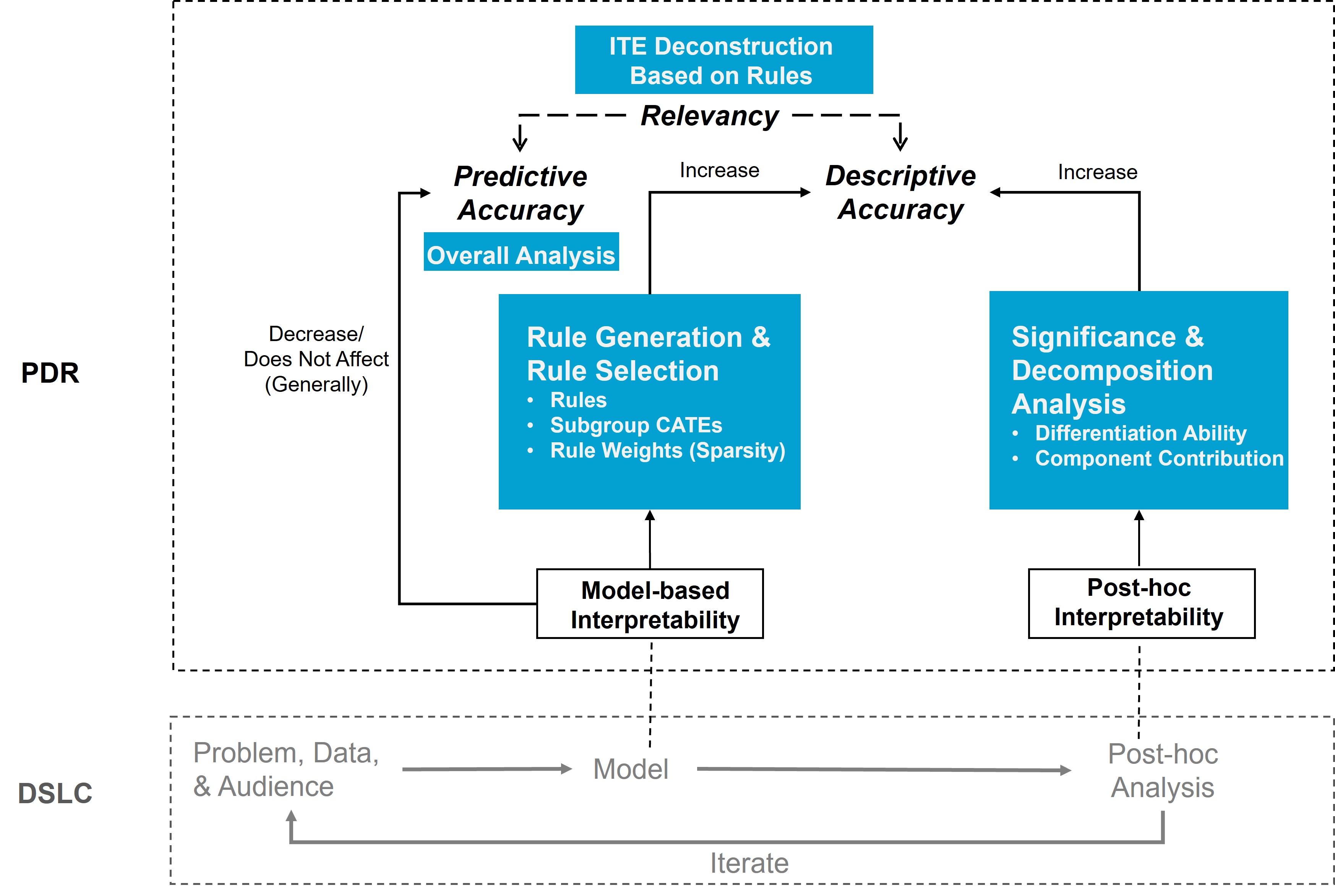
Figure 1: Overview of the PDR framework of interpretability in different stages where interpretation matters in the data-science life cycle (Murdoch et al., 2019). How CRL enables PDR interpretability is also shown and highlighted in blue texts.

Motivated by the PDR framework for interpretability, we propose causal rule learning (CRL for short), a rule-based workflow to enable interpretable estimation of HTE. To cater to the needs of physicians and achieve the relevancy desiderata with CRL, we adopt a novel but practical perspective of HTE by deconstructing ITE into a linear combination of subgroup CATEs. The subgroups are characterized by rules due to their easiness in human understanding, usefulness in healthcare practice, and inclusion of potential knowledge. This perspective is actually an assumption that delves deeper into a potential inner structure of ITE by connecting it with the subgroup level treatment effect. It attempts to answer a practical question that is highly relevant to healthcare practice yet has seemingly never been asked before: What if an individual belongs to multiple subgroups with different characterizing features and CATE estimates simultaneously?

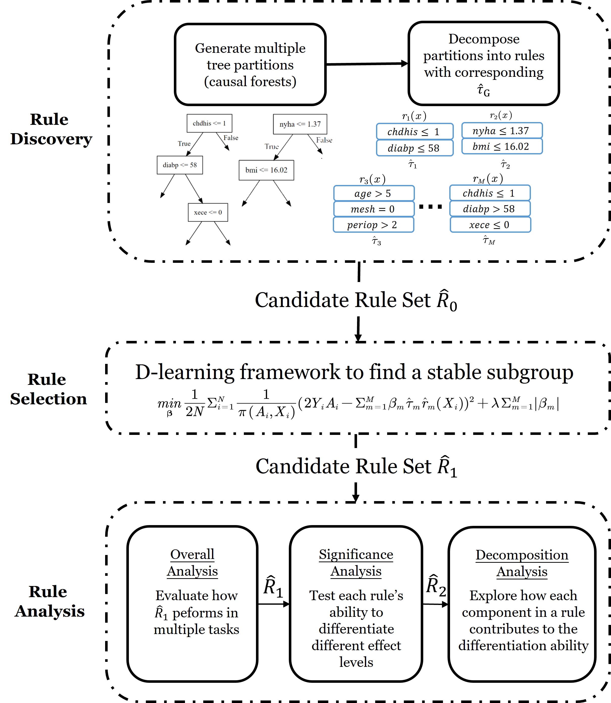
Figure 2: Workflow of causal rule learning.

CRL incorporates three steps, i.e., rule discovery, rule selection, and rule analysis, to enable the above perspective and to achieve both model-based and post-hoc interpretability. Specifically, the rule discovery step first generates a set of rules and their corresponding subgroup CATE estimates using causal forest (Wager and Athey, 2018). Then, the rule selection step leverages a D-learning method (Qi et al., 2018) to filter out non-informative rules and uses the informative ones to estimate ITE. The sparsity imposed on the rule set makes it more feasible for human interpretation and further analysis. The rules, related subgroup CATEs, and weights learned from the first two steps provide the desired model-based interpretability. Next, the rule analysis step focuses on evaluating the rules from three different views, including the overall analysis, significance analysis, and decomposition analysis. In detail, the overall analysis investigates how the D-learning rule set performs in different HTE-related tasks and shows our model’s predictive accuracy. The significance analysis then tests how significant each rule is to distinguish different levels of ITE, and the decomposition analysis explores each component’s contribution in a rule to its differentiation ability. The last two analyses provide post-hoc interpretability to increase descriptive accuracy further, showing more insights into each specific rule. For a more straightforward representation, how the proposed CRL workflow enables the PDR interpretability is reflected in Figure 1 with white texts in blue colored blocks. The whole workflow of CRL with details is also shown in Figure 2.

We demonstrate the superiority of CRL using both simulated and real-world data. Results show that CRL is able to provide both comparable accuracy and enhanced interpretability in the estimation of HTE and other related tasks when the underlying ground truth is complex and the sample size is sufficient.

Our work enriches the toolkits of HTE estimation with a high level of interpretability. To our knowledge, this is what lacks in existing relevant literature and deserves more attention from the community. Under the guidance of PDR, we enhance our understanding of HTE by i) adopting an enlightening perspective that links group level and individual level treatment effect and ii) designing a comprehensive workflow to implement this perspective, with in-depth analysis of the identified rules. The rules that survive in all the analyses may suggest potential knowledge and can be examined with more rigorous statistical methods and validation through experiments in specific domains.

The rest of this paper is organized as follows: In Section 2, we briefly summarize previous studies on HTE. Section 3 delineates the proposed CRL method in detail, including its basic data settings, assumptions, formulation, and workflow. Section 4 and 5 demonstrate the power of CRL with simulated randomized controlled trial (RCT) data sets and real-world observational data sets, respectively. Section 6 concludes our work, and discusses our work’s limitations and potential future directions. For brevity in this paper, we will abuse the following terms slightly: i) HTE, CATE, and ITE; ii) satisfy a rule and belongs to a subgroup. These terms are used according to specific contexts and sometimes indiscriminately in broader situations.

2 Related work

This section presents three parallel streams of literature related to this work. They are CATE/ITE estimation, subgroup identification, and optimal policy learning.

The CATE/ITE estimation perspective focuses on developing conditional treatment effect estimators with favorable statistical properties, including parametric models that often make assumptions on the function form of treatment effect (Chen et al., 2015; Su et al., 2009) and non-parametric methods that model more complex relationships between treatment, covariates, and outcome of interest, such as tree-based methods (Athey and Imbens, 2016; Green and Kern, 2012), forest-based methods (Athey et al., 2019; Wager and Athey, 2018), and meta-learning frameworks (He et al., 2022; Polley et al., 2011; van der Laan and Rose, 2011). There also exist many relatively complex methods, creating significant obstacles for practitioners’ understanding, such as Balancing Neural Networks (Johansson et al., 2016), Deep Counterfactual Networks (Alaa et al., 2017), Causal Multi-task Gaussian Processes (Yoon et al., 2018) and Non-stationary Gaussian Processes model (Alaa and Schaar, 2018).

Subgroup identification emphasizes identifying and characterizing subgroups with statistically significant and practically meaningful heterogeneity in treatment response. To this end, recursive partitioning-based methods are popular due to their advantages in heuristic population segmentation (see, e.g., Lipkovich et al., 2011; Seibold et al., 2016; Su et al., 2009). Unlike these, the patient rule induction method (PRIM) utilizes a bump hunting search with the objective function targeted at the significance of treatment effect of potential subgroups (Chen et al., 2015). Sequential bootstrapping and aggregating of the threshold from trees (Sequential-BATTing) shares the same objective function used in PRIM but iterates the candidate subgroup through a BATTing search (Huang et al., 2017b).

A few notable rule-based methods have emerged in this topic, following quite different philosophies and workflows. For example, Dwivedi et al. (2020) propose Stable Discovery of Interpretable Subgroups via Calibration (StaDISC). This method discovers interpretable and stable rule sets from well-calibrated samples on 18 popular CATE estimators. Wang and Rudin (2022) propose Causal Rule Sets (CRS) to identify subgroups with enhanced treatment effect through a generative Bayesian framework that assumes a prior for the actual rule set and a Bayesian logistic regression model to improve it. Bargagli-Stoffi et al. (2023) provide the Causal Rule Ensemble (CRE) method to identify meaningful subgroups through a greedy search of potential rules. Specifically, they split data into two parts: discovery sample for rule discovery with existing methods and inference sample for CATE estimation. A rule regularization and a sensitivity test are performed for interpretability concern and robust estimation, respectively.

Optimal policy learning, or more generally treatment recommendation, focuses on directly modeling the best-individualized treatment policy given personal characteristics to maximize the outcome of interest. For static decision problems, there are weighting models like outcome weighted learning (OWE) (Zhao et al., 2012) and residual weighted learning (Zhou et al., 2017), and subgroup-based models (Foster et al., 2011; Seibold et al., 2016; Yu et al., 2023). For chronic disease management, which requires sequential decision-making, many methods leverage the reinforcement learning related models, such as quality-learning (Qian and Murphy, 2011; Schulte et al., 2014), advantage-learning (Murphy, 2003; Schulte et al., 2014), and partially observable Markov decision process (Gong and Liu, 2023; Skandari and Shechter, 2021).

All the above three streams are ways to explore HTE and support various degrees of personalized decision making. There is no clear boundary between these three streams, and it is easy to find that many of the methods mentioned above can be used for all purposes. CATE/ITE estimation is treatment effect estimation on more granular subsets of the population, i.e., subgroup level or individual level. Optimal treatment is often determined by the sign of CATE/ITE, whether indicated explicitly (Verbeke et al., 2023) or implicitly (Qi et al., 2018). Our work can be classified into the CATE/ITE estimation category, concerned about the interpretability issue in its estimation. Due to the connection between the three streams, our method can also be used in the other two tasks, as we show later.

3 Causal Rule Learning

3.1 Notation and assumptions

We consider a triplet $\{X,A,Y\}$ where $X=(x_{1},x_{2},\dots,x_{p})^{\top}$ denotes a $p$-dimensional vector of sample characteristics (covariates), $A\in\mathcal{A}=\{-1,1\}$ represents the treatment received with value 1 as positive treatment and -1 as negative treatment (or control). $Y(1)$ and $Y(-1)$ denote the potential outcomes of receiving positive and negative treatments, respectively. Suppose that we have observed a data set $\mathcal{D}=\{X_{i},A_{i},Y_{i}\}^{N}_{i=1}$ which comprises $N$ independent and identically distributed (IID) samples. $Y_{i}=Y(A_{i})\in\mathbb{R}$ is the observed outcome that higher values are preferred.

The above data set may come from an observational study or, more ideally, a Randomized Controlled Trial (RCT) setting. Our method can be applied to data from both settings but requires the satisfaction of the three basic assumptions of the Neyman–Rubin potential outcome framework (Rubin, 1980; Rosenbaum and Rubin, 1983), namely the Stable Unit Treatment Value Assumption (SUVTA), unconfoundedness assumption, and overlap assumption. Details of these assumptions are given in A. Besides, both the unconfoundedness assumption and our formulation of D-learning (model (6)) leverage the propensity score defined as the probability of receiving treatment $a$ given $X$, i.e., $\pi(a,x)=Pr(A=a|X=x)$, so we have to know this score in advance. RCT setting is considered to satisfy the above three assumptions automatically, and the propensity score is already known. For observational data, checking SUVTA is relatively easy. What is more important is to estimate from the data a proper propensity score model and check the overlap of samples before the application of CRL, as we will show in the real-world data analysis in Section 5 and C.

3.2 Individualized treatment effect based on causal rules (subgroup CATE)

The true ITE of instance $i$ is $Y_{i}(1)-Y_{i}(-1)$, a quantity that is never observable due to the absence of counterfactual outcomes. In this study, we estimate this quantity of interest through a set of causal rules rather than modeling counterfactual outcomes.

First, a rule is an if-then statement: IF condition THEN conclusion. Rules match our needs for accuracy and interpretability for the following reasons: i) As a natural way to represent knowledge, rule is easy to understand and modify. It uncovers variables’ potential interaction (synergistic effect) and defines a certain subpopulation to help us understand the heterogeneity of treatment effect. ii) Rule has already formed the daily routine of healthcare practice, such as clinical guidelines. For human experts, it is easy to simulate and reason about the entire decision process with rules (Murdoch et al., 2019). iii) Friedman and Popescu (2008) and Murdoch et al. (2019) show evidence that rule-based models have comparable and sometimes even better performance than black box methods like neural networks. We formulate a rule as follows:

$$r(x)=\prod_{j=1}^{p}{1}(x_{j}\in s_{j}),$$ (1)

where $x_{j}$ denotes the $j$-th element of $x$, $s_{j}$ is a specified subset of all values of $x_{j}$, and $\mathop{1}(\cdot)$ is the indicator function yielding 1 when $x_{j}\in s_{j}$ and 0 otherwise. Thus, a rule $r(x)$ maps an input $x$ into $\{0,1\}$, representing the satisfaction of a rule with 1 and 0 otherwise.

By causal rules, we mean that the rules are identified from a causal inference framework. As a rule defines a specific subgroup of the whole population, we can derive its subgroup CATE simply from the difference in the expectation of outcomes between the positive and negative treatment samples in this subgroup, i.e.,

$$\tau_{G}=\mathbb{E}[Y|A=1,X\in G]-\mathbb{E}[Y|A=-1,X\in G],$$ (2)

where $G$ is the feasible subset of feature space values defined by the particular subgroup. Suppose the true rule set has $M$ rules (subgroups). Our method assumes that the true ITE can be formulated through a linear combination of all the CATEs corresponding to the subgroups the individual belongs to:

$$\tau(x):=\sum_{m=1}^{M}\beta_{m}\tau_{m}r_{m}(x),$$ (3)

where $r_{m}(x)$, $\tau_{m}$, and $\beta_{m}$ denote the satisfaction of the $m$-th rule given $X=x$, its corresponding subgroup CATE and true weight in the linear combination. This formulation shows a novel rule-based (or subgroup-based) perspective to interpret ITE, which connects treatment effect on both subgroup and individual levels.

Imagine that multiple true subgroups have distinct characteristics and magnitude of treatment effects. Then, assumption (3) tries to answer a very practical question: What if an individual belongs to different subgroups simultaneously? Each subgroup CATE has a different contribution to ITE, reflected through the sign and magnitude of the weights $\mathrm{\beta}$ and the subgroup CATEs. More significant absolute values of these quantities imply more contribution. Given above, the problem then boils down to the revelation of $\{r_{m}(x),\tau_{m},\beta_{m}\}^{M}_{m=1}$. Various methods can be used to find the rules and estimate the quantities. The final choice is up to the particular problem and intended audience. The next section shows our CRL framework to achieve these goals.

3.3 CRL Workflow

3.3.1 Rule discovery via causal forest

Our model utilizes causal forests (Wager and Athey, 2018) to derive the initial set of potential rules and corresponding CATE estimates. The causal forest is a non-parametric method for heterogeneous treatment effect estimation whose estimator has been shown to have good statistical properties like point-wise consistency and asymptotical normality for the true CATE under certain conditions.

A causal forest consists of many causal trees (Athey and Imbens, 2016), each trained with a random subsample of observations and covariates. In detail, a tree $\Pi$ is defined as

$$\Pi=\{l_{1},\dots,l_{\#(\Pi)}\}$$

with $\cup_{m=1}^{\#(\Pi)}l_{m}=\mathbb{X}$ the feature space, $\#(\Pi)$ denotes the number of elements (leaf nodes) in the tree and $l(x;\Pi)$ denote the leaf that $x$ belongs to. In the causal tree algorithm, one performs an honest estimation that divides all samples into three parts for three purposes, i.e., training set $S^{tr}$ to construct the tree partition, estimation set $S^{est}$ to estimate the treatment effects within each leaf node of the tree, and test set $S^{te}$ to evaluate the performance of the learned tree. This process guarantees the independence of tree partition learning and effect estimation. The splitting criterion of the classic classification and regression tree (CART) (Loh, 2011) algorithm is adjusted and estimated precisely for treatment effect estimation where the true CATE can never be observed.

Given a causal tree, it is easy and intuitive to decompose the tree into multiple rules: the path from the root to a leaf node naturally forms a rule formulated in definition (1) where $x_{j}$ can be the $j$-th node (except the leaf) in the path and $s_{j}$ represents the subset of feasible values $x_{j}$ takes to go along the path. Therefore, a leaf node directly represents a potential subpopulation defined with these splitting variables. Further, we use the following plug-in estimator of difference-in-means as the corresponding CATE of a subgroup $G$:

$$\hat{\tau}_{G}=\frac{\sum_{i}Y_{i}{1}(A_{i}=1,X_{i}\in G)}{\sum_{i}{1}(A_{i}=1,X_{i}\in G)}-\frac{\sum_{i}Y_{i}{1}(A_{i}=-1,X_{i}\in G)}{\sum_{i}{1}(A_{i}=-1,X_{i}\in G)}.$$ (4)

3.3.2 Rule selection with the D-learning method

Due to the randomization and greediness introduced by forest-based methods, fake and redundant rules are inevitably generated (Bargagli-Stoffi et al., 2023; Wang et al., 2020). The rule selection process aims to filter out those irrelevant and unnecessary rules from the initial rule set to improve the accuracy of ITE estimation and size down the set for interpretability purpose.

Now, we introduce the D-learning method (Qi et al., 2018) to learn a sparse combination of rules that can estimate ITE accurately. The original D-learning method aims to directly learn the optimized individual treatment rule (ITR) $d^{*}(x)$ in a single step without model specification, defined as follows:

$$d^{*}(x)=\textnormal{sign}\Big{(}\mathbf{E}\Big{[}\frac{YA}{\pi(A,X=x)}\big{|}X=x\Big{]}\Big{)}=\textnormal{sign}(\tau^{*}(x)).$$ (5)

Obviously, the expectation $\mathbf{E}[YA/\pi(A,X=x)|X=x]$ or $\tau^{*}(x)$ is the exact desired ITE.

It has been proved in Qi et al. (2018) that under certain assumptions,

$$\tau^{*}(x)\in\mathop{\arg\min}_{\tau(x)}\mathbf{E}\Big{[}\frac{(2YA-\tau(x))^{2}}{\pi(A,X=x)}|X=x\Big{]},$$

where $\tau(x)$ can be any proper form. This proof makes it possible to transform the estimation of unobserved ITE into a supervised learning problem where the ground truth $Y$ is already known. It also allows the specification of flexible forms for $\tau(x)$, whether linear or nonlinear. As indicated in formula (3), we specify a linear combination of subgroup CATE to characterize $\tau(x)$ and impose additional $\ell_{1}$ penalty on the weights of the rules to ensure sparsity. By replacing the expectation term in $\tau(x)$ with empirical mean, we formulate the estimation of $\tau^{*}(x)$ as a $\ell_{1}$ penalized regression problem:

$$\hat{\mathbf{\beta}}^{lasso}=\arg\min_{\mathbf{\beta}}\Big{\{}\frac{1}{2N}\sum^{N}_{i=1}\frac{1}{\pi(A_{i},X_{i})}\{2Y_{i}A_{i}-\sum_{m=1}^{M}\beta_{m}\hat{\tau}_{m}\hat{r}_{m}(X_{i})\}^{2}+\lambda\sum_{m=1}^{M}|\beta_{m}|\Big{\}},$$ (6)

where $\lambda$¿$0$ is the tuning parameter that controls the degree of $\ell_{1}$ penalty. Solving this minimization problem gives us the least absolute shrinkage and selection operator (LASSO) estimator (Tibshirani, 1996) of rule weights $\hat{\mathbf{\beta}}^{lasso}$. Then we can easily obtain CRL estimates of ITE: $\hat{\tau}_{CRL}(x)=\sum_{m=1}^{M}\hat{\beta}^{lasso}_{m}\hat{\tau}_{m}\hat{r}_{m}(x)$.

Just as Murdoch et al. (2019) states, when we impose sparsity on our model, we limit the number of non-zero parameters in the model and interpret the rules corresponding to those parameters (through sign and magnitude) as being meaningful to the outcome of interest. Since a large number of weights are zero (i.e., $\hat{\beta}^{lasso}$ has many elements equal to 0), their corresponding rules are actually removed from the candidate set and make no contribution to our estimator. Imposing this sparsity of rules also highlights the distinction between our CRL estimator and the causal forest estimator: Causal forest takes the simple average over all the tree estimates (subgroup CATEs in our method) as the final estimates while our method learns a weighted combination of the estimates. In other words, we reweight the tree estimates instead of using them equally. In this sense, causal forest estimates can be viewed as a special case of our method. We show in Figure 5 that the reweighting is able to eliminate a large proportion of unwanted rules generated by causal forest.

3.3.3 Rule analysis

Interpreting our estimated $\tau(x)$ relies on understanding the subgroups contributing to it. A comprehensive analysis of the subgroups identified is what needs to be improved in existing studies. This analysis is indispensable since i) we cannot guarantee that all the rules selected by the previous step have their stated impact on our estimators, and ii) the size of the rules may still be too large to achieve human comprehension. Thus, we show a procedure to analyze further the rules remaining in the candidate set to find a relatively smaller yet more promising subset of rules. For clarification, this procedure continues to remove a bunch of rules, but mainly for interpretability purpose, and the estimation of ITE is still made on all the rules D-learning selects (rules with non-zero weights). This procedure includes but is not necessarily limited to the following three parts: overall analysis, rule significance analysis, and rule decomposition analysis. Unlike previous studies, our analysis does not focus on the subgroups with higher treatment effects but on those with significantly different ITE estimates, whether higher or lower.

Overall analysis. Suppose D-learning selects a rule set consists of $n_{1}$ rules ($n_{1}\leq M$) whose weights are non-zero in model (6), i.e., , $\hat{R}_{1}=\{\hat{r}_{1},\hat{r}_{2},\dots,\hat{r}_{n_{1}}\}$ (for simplicity, we use $\hat{r}_{j}$ instead of $\hat{r}_{j}(x)$ to represent a rule). The corresponding CRL estimates of ITE $\hat{\tau}_{CRL}$ are also obtained based on this rule set. As predictive accuracy is the basis of interpretability, the overall analysis aims to evaluate how this rule set performs from the three perspectives of HTE research we discussed before. For a more straightforward evaluation, we can compare the results of CRL with those of other baseline methods in each task using various performance metrics below.

For CATE/ITE estimation, we can evaluate how accurately our method estimates the true ITE using Mean Squared Error, i.e., , $MSE(\hat{\tau})=N^{-1}\sum^{N}_{i=1}(\hat{\tau}(X_{i})-\tau(X_{i}))^{2}$, where $\hat{\tau}(X_{i})$ and $\tau(X_{i})$ are a certain estimate and the true ITE of instance $i$ respectively. The smaller the value, the better an estimator does.

For treatment recommendation, we measure the mean potential outcomes under a certain method’s treatment assignment based on the sign of its ITE estimates. We can use Mean Potential Outcomes (MPO), defined as $M(d)=N^{-1}\sum^{N}_{i=1}{Y_{i}(d(X_{i}))}$ where treatment assignment $d(X_{i})=1$ if $\hat{\tau}(X_{i})$¿0 and $-1$ otherwise for instance $i$. The bigger the value of MPO, the better the estimator.

For subgroup identification, we can evaluate the proportion of true rules in a given rule set using Proportions of true rules (POTR) defined as ${|T\cap I|}/{|I|}$ where $T$ denotes the set of true rules and $I$ is a certain candidate rule set, say, $\hat{R}_{1}$. $|\cdot|$ is the number of rules in a set. However, sometimes, the true rule consists of continuous covariates whose cut-off values cannot be exactly recovered, and it may be challenging to find a reasonable range of acceptable cut-off values for the variable. Therefore, we convert to the instances a rule set covers, rather than the accuracy of a specific rule representation, and define Population overlap (PO)=${|T^{\prime}\cap I^{\prime}|}/{|T^{\prime}\cup I^{\prime}|}\in[0,1]$. $T^{\prime}=\{i\in N|\tau(X_{i})$¿$0\}$ and $I^{\prime}=\{i\in N|\hat{\tau}(X_{i})$¿$0\}$, representing respectively the sets of instances whose true ITE and estimated ITE are positive. This measure tests the degree of intersection of the two groups. When $T^{\prime}\cap I^{\prime}=\emptyset$, $PO=0$ and when $T^{\prime}=I^{\prime}$, $PO=1$. Bigger values are preferred.

For quick reference, the above performance metrics defined in each perspective are summarized in Table 1, column 2. Note that these metrics are designed for simulated data where the true ITE is already known. For real-world observational data, we define relevant metrics in column 3 and introduce them in detail in Section 5.

Suppose the above overall analysis shows that our methods are able to give comparable or acceptable results to baseline methods. In that case, we continue the following analysis, which evaluates each rule in terms of i) the ability to distinguish different levels of ITE, i.e., rule significance, and ii) the role of each component in the rule, i.e., rule decomposition analysis.

Rule significance analysis. A rule defines two subpopulations: the population that satisfies the rule $G^{Y}=\{i|r(X_{i})=1\}$ and the rest that does not $G^{N}=\{i|r(X_{i})=0\}$. Therefore, we want to test the discriminating power of a rule by checking if $G^{Y}$ and $G^{N}$ differ significantly in the magnitude of ITE estimates, using the well-known two-sample Kolmogorov–Smirnov test (Berger and Zhou, 2014). A $p$-value $\leq 0.05$ implies that the rule can identify a subgroup with significantly different treatment effects than the rest of the population. We perform this test on each rule in $\hat{R}_{1}$ and remove those with $p$-value $>0.05$. The remaining $n_{2}$ rules ($n_{2}\leq n_{1}$) form the new candidate rule set $\hat{R}_{2}$.

Rule decomposition analysis. Decomposition analysis evaluates how each component (variables and the cut-off values) in a rule contributes to the complete rule in differentiating treatment effect. Specifically, for a certain rule $\hat{r_{j}}$ with three components $a$, $b$ and $c$, we can derive three revised rules: $\hat{r}^{a}_{j}$, $\hat{r}^{b}_{j}$ and $\hat{r}^{c}_{j}$. $\hat{r}^{a}_{j}$ is the rule with component $a$ removed from the original rule, that is, the rule formed only by component $b$ and $c$ and similarly for $\hat{r}^{b}_{j}$ and $\hat{r}^{c}_{j}$. We do the above significance analysis on all revised rules and obtain their corresponding $p$-values $p^{a}_{j}$, $p^{b}_{j}$ and $p^{c}_{j}$. We think a higher $p$-value of the revised rule than that of the original complete rule, say, $p^{c}_{j}$¿$p_{j}$, implies that the revised rule $\hat{r}^{c}_{j}$ is less significant in distinguishing subpopulations with different levels of ITE estimates than the original entire rule $\hat{r_{j}}$. Hence, the removed component $c$ contributes to the significance of ITE difference. The higher the $p$-value of the revised rule, the more critical the variable being removed is, which reveals the variable most accountable for the group’s heterogeneity. In contrast, a lower value suggests the corresponding component(s) may be unnecessary and meaningless to the complete rule since its removal does not reduce the significance of the difference but increases it. Therefore, if all revised rules have higher $p$-values ($p_{j}$¡$min\{p^{a}_{j},p^{b}_{j},p^{c}_{j}\}$), then all the components in the rule work synergistically to contribute to its discriminating power. In this step, we retain the rules that have higher $p$-values on all the corresponding revised rules to form a new refined set $\hat{R}_{3}$ with $n_{3}$ rules ($n_{3}\leq n_{2}$).

In conclusion, we show a universal way to analyze the identified rules and subgroups. However, these tools highly rely on the data in hand. Therefore, we recommend using this analysis procedure as a screening step for the lengthy list of rules and picking out the top subgroups for more desirable interpretation through other possible tools and domain analysis.

4 Simulation study

In order to evaluate how well CRL performs to estimate and improve our understanding of HTE, we perform the following two studies with different goals and setups. The first set of experiments tests the overall performance of CRL. The second set evaluates specifically the rule selection step of CRL, that is, to test whether D-learning is able to identify the true pre-defined subgroups from a pool of candidates.

4.1 Study one: overall performance of CRL

In this study, we test the overall performance of CRL. Specifically, we first generate simulated RCT data sets $\{X_{i},A_{i},Y_{i}\}_{i=1}^{N}$ based on assumption (3). Then we run the entire CRL workflow and compare it with several before-mentioned baseline methods, namely OWE (Zhao et al., 2012), PRIM (Chen et al., 2015), SEQBT (Huang et al., 2017b), and Causal Forest (Wager and Athey, 2018).

4.1.1 Data setups

We generate covariates $X\in\mathbb{R}^{9}$ where the first three elements (features) $x_{1},x_{2}$, and $x_{3}$ are randomly drawn from $\{0,1\}$ with equal probability ($x_{3}$ is sampled differently for some setups of the true group, shown later).

The last six features are $\{x_{j}|j=4,5,\dots,9\}\overset{\mathrm{i.i.d}}{\sim}\mathcal{N}(0,2)$. For simplicity, we ignore the sample foot notation $i$ and the remaining footnote specifies certain features unless otherwise noted. The baseline effect is defined as $f(X)=1+x_{1}+2x_{6}+3x_{2}x_{3}+5x_{4}x_{7}+4x_{5}x_{8}$.

Based on assumption (3), we can define any number of true subgroups and their related true CATEs via a rule form (shown later). Once we set the true $\tau(X)$, we define the potential outcomes for both the negative and positive treatments: $Y(-1)=f(X)+\epsilon$ and $Y(1)=Y(-1)+\tau(X)$, where $\epsilon\sim\mathcal{N}(0,1)$. We imitate the simplest RCT assignment of the treatment arm: $A_{i}$ is sampled from $\{-1,1\}$ with equal probability. Therefore, the observed outcome in our data set is $Y_{i}=2^{-1}(1+A_{i})Y_{i}(1)+2^{-1}(1-A_{i})Y_{i}(-1)$.

To sum up, the observed data set $\{X_{i},A_{i},Y_{i}\}^{N}_{i=1}$, together with the predefined baseline effect $\{f(X_{i})\}^{N}_{i=1}$ and true ITE $\{\tau(X_{i})\}^{N}_{i=1}$ forms the basis of the ground truth of the data generation. To avoid randomness and to test how the performance of CRL changes with the data settings, we make a few variations to our simulated data:

• Number of the observations (num.obs) $N\in\{5000,10000\}$,

• Effect size base quantity $k\in\{5,10,15,20,25,30\}$, where $k$ is used in the definition of true subgroups and related $\tau$ in Figure 3,

• Number of true positive subgroups (num.grp) defined in rules: $M^{*}\in\{1,3,5\}$. If $M^{*}=5$, $x_{3}\sim U(0,10)$, otherwise, it still follows the before-mentioned Bernoulli distribution. For a clearer performance comparison, we focus on identifying subgroups whose true treatment effects are positive (i.e., true positive subgroups) which most baseline methods only care about. However, we keep the pre-defined negative groups in our setups.

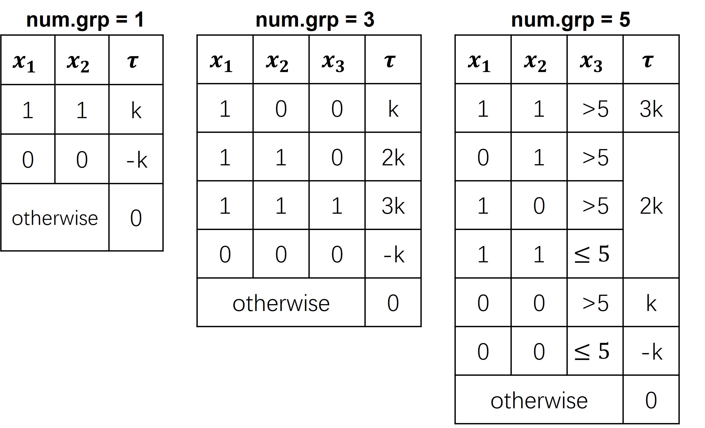
Figure 3: Specification of true treatment effect $\tau(x)$ for varying numbers of subgroups. E.g., for num.grp = 3, $\tau=k$ if $x_{1}=1,x_{2}=0$ and $x_{3}=0$.

Table 1: Overview of the model evaluation metrics in overall analysis.

Perspectives	Simulated data	Real-world data
CATE/ITE estimation	$MSE(\hat{\tau})=N^{-1}\sum^{N}_{i=1}(\hat{\tau}(X_{i})-\tau(X_{i}))^{2}$	ITE-based outcome accuracy
Treatment	Mean potential outcomes:	Empirical value function:
recommendation	$M(d)=N^{-1}\sum^{N}_{i=1}{Y_{i}(d(X_{i}))}$	$\hat{V}(d)=\frac{\mathbf{E}_{n}[Y1(A=d(X))/\pi(A,X)]}{\mathbf{E}_{n}[1(A=d(X))/\pi(A,X)]}$
Subgroup identification	Proportion of true rules: $\frac{|T\cap I|}{|I|}$	Treatment efficient frontier
	Population overlap: $\frac{|T^{\prime}\cap I^{\prime}|}{|T^{\prime}\cup I^{\prime}|}$

Together, we have $2\times 3\times 6=36$ data sets. We first make 100 re-sampled repetitions for each data set and randomly split each repetition into a 70% training set and 30% test set. Then, we apply the overall CRL workflow as well as other baseline models on the training data and report the performance metrics on the test data, averaging over 100 repetitions. See B.0.1 for the details of CRL parameter tuning on each data. Baseline methods are implemented with R package personalized (Huling and Yu, 2021) for OWE, subgrpID (Huang et al., 2017a) for PRIM and SEQBT, and grf (Tibshirani et al., 2022) for causal forest.

4.1.2 Simulation results

This section compares the results of fitting CRL and other baseline methods with the 36 data sets through the three perspectives indicated in section 3.3.3. Since the baseline methods vary in research focus and model outputs, not all methods are compared for all performance metrics.

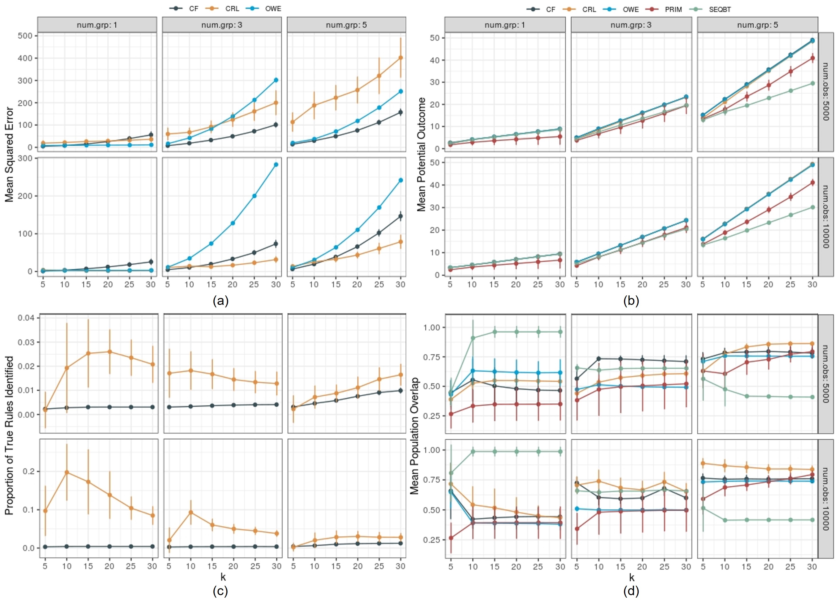
Figure 4: Performance comparison of CRL and other baseline methods applied on the simulated data in study one. Results are averaged over 100 repetitions for each data set. (a) Mean squared error of treatment effect $MSE(\hat{\tau})$. (b) Mean potential Outcome. (c) Proportions of true rules identified. OWE does not give explicit rules and PRIM fails to reveal even one rule, thus we do not include their results in this figure. (d) Mean population overlap.

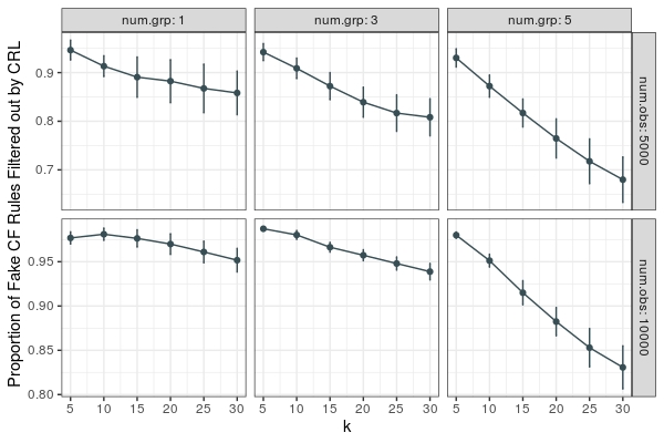
Figure 5: Proportion of fake rules generated by CF and then filtered out by CRL, averaged over 100 repetitions for each data.

ITE estimation. Figure 4(a) shows the MSE of ITE estimates (with one standard error bar) averaged over 100 repetitions of each data set. From top to bottom, the number of observations of the data set varies from 5,000 to 10,000, and from left to right the number of true positive subgroups from one to five. Effect size ($k$) is reflected in the x-axis of each subfigure (similarly for the following figures). Reasonably, each method’s MSE increases as the effect size gets large in different setups. When $N=5000$, CRL (orange curve) is inferior to other methods in terms of the MSE, and this disadvantage increases gradually as the number of true subgroups grows. On the contrary, CRL beats other methods when $N=10,000$, with lower MSE and smaller variance (e.g., $k=15,20,25,30$) compared to OWE and causal forest (CF).

Treatment recommendation. Figure 4(b) indicates that CRL, CF, and OWE show almost the same good performance on MPO and outperform SEQBT and PRIM in all settings. The identical performance of CRL, CF, and OWE is a result of our treatment assignment strategy: we recommend treatment only according to the sign of the estimated ITE. Regardless of how these methods differ in the magnitude of the estimates, they yield identical treatment recommendations as long as their estimates have identical signs and hence the same values on MPO.

Subgroup identification. Since CRL filters out rules from the original rule set derived from CF, we first evaluate the percentage of fake rules eliminated during the CRL filter process using Proportion of CF rules filtered out by CRL. This metric is defined as $1-{W_{CRL}}/{W_{CF}}$ where $W_{CRL}=|\{r_{m}|r_{m}\in I_{CRL},r_{m}\notin T\}|$ represents the number of fake rules in the rule set identified by CRL, $I_{CRL}$, and similarly $W_{CF}$ by CF. The bigger the value, the better CRL filters out fake rules. As indicated in Figure 5, through the additional D-learning selection and rule analysis procedure, CRL is able to filter out a higher proportion of fake rules generated by CF. Hence CRL has a higher proportion of true rules (POTR) in its final rule set than that of CF, shown in Figure 4(c).

Figure 4(d) demonstrates that CRL consistently identifies more true samples with positive ITE than other methods when $N=10,000$ under three or five true groups, with bigger overlap value and lower variance. This is also the case for most effect magnitudes $k$ under five true groups when $N=5,000$.

Generally, Figure 4 clearly demonstrate CRL’s advantage with regard to all three tasks when the underlying ground truth is complex and we have a sufficient size of observations. Moreover, CRL gives us more explicit rules than OWE, more refined rules than CF, and more potential options of rules than PRIM under proper scenarios.

4.2 Study two: rule selection performance

This study simply tests how well D-learning identifies the true pre-defined subgroup. Given a candidate rule set including the pre-defined true rules and fake rules with corresponding subgroup CATEs, is the subsequent D-learning method able to discover all the true rules?

First, we define the rule satisfaction matrix, where each row represents a sample and each column a rule. The element $(i,j)=1$ indicates that sample $i$ satisfies rule $j$ and 0 otherwise. This matrix is then used in the LASSO problem as raw input. We define the true rules to be the 10-th, 20-th, 30-th, 40-th and 50-th rules and the subgroup CATEs $\tau_{m}=k$ if $m\in\{10,20,30,40,50\}$ and $\tau_{m}\sim\mathcal{N}(0,1)$ otherwise. Then, we define the true ITE as $\tau(X)=0.1\tau_{10}r_{10}(X)+0.2\tau_{20}r_{20}(X)+0.3\tau_{30}r_{30}(X)+0.4\tau_{40}r_{40}(X)+0.5\tau_{50}r_{50}(X).$

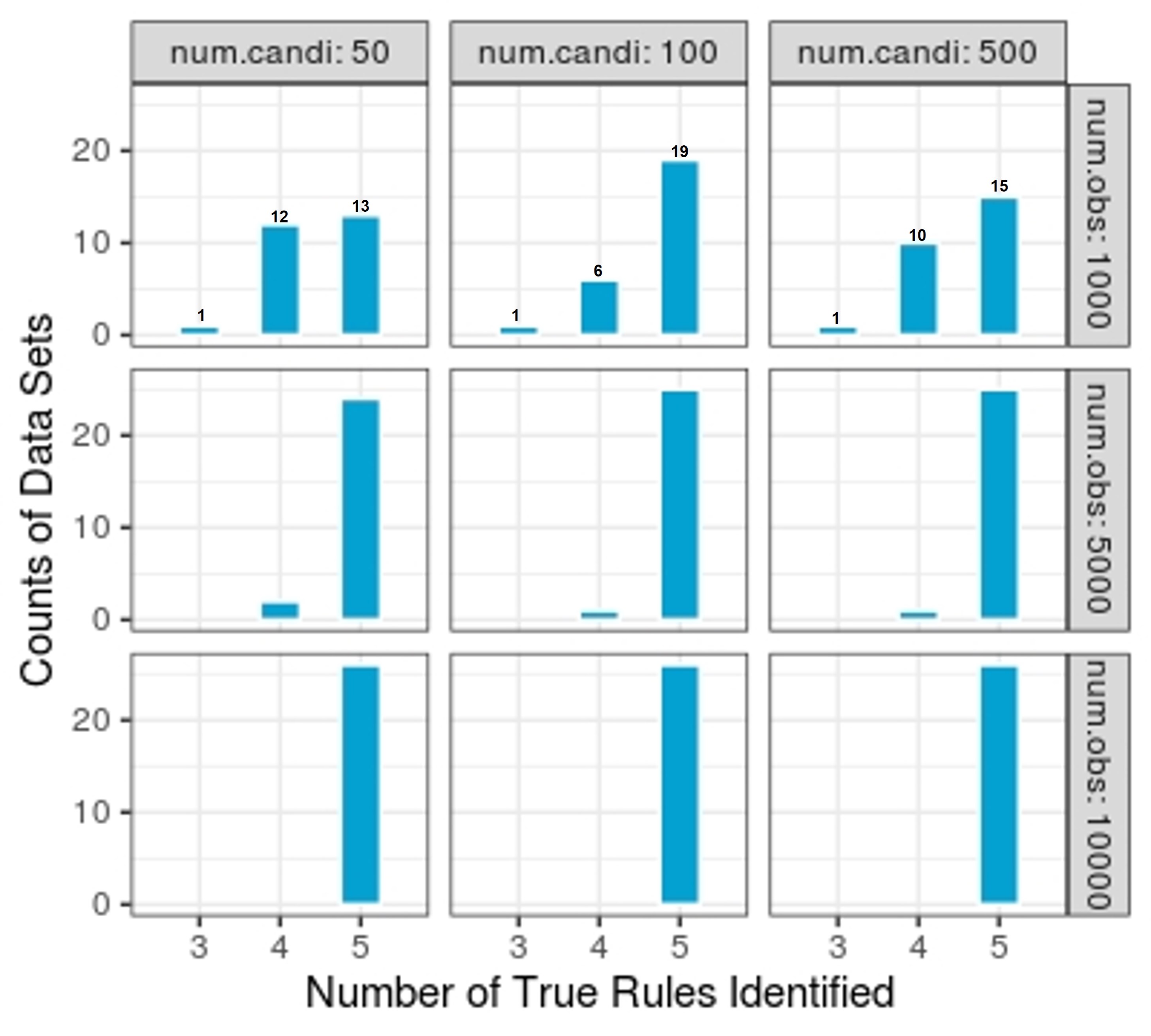
Figure 6: The counts of data sets for which CRL successfully uncovers the true rules using D-learning, stratified by the number of true rules identified.

We vary the true setting by the number of candidate rules (num.candi) $M\in\{50,100,500\}$ (i.e., the number of columns of rule satisfaction matrix to be 50,100 and 500), the number of observations $N\in\{1000,5000,10,000\}$ and $k$ to be all the integers between 5 and 30 (26 values). We have nine settings in total. For each specific setting, say, number of candidate rules = 50 and number of observations = 1,000, we have 26 data sets. We sample the treatment variable $A$ from $\{-1,1\}$ with equal probability. Potential outcome $Y(-1)$ is sampled from $N(0,10)$ and $Y(1)=Y(-1)+\tau(X)$. The observed outcome is still $Y=2^{-1}(1-A)Y(-1)+2^{-1}(1+A)Y(1)$.

For each setting, we summarize how many (the counts of) data sets out of the 26 ones for which CRL successfully identifies certain number of true rules (three and above) using D-learning, shown in Figure 6. The top left subfigure shows that CRL uncovers all five true rules on 13 data sets, four true rules on 12 data sets, and three on the remaining one data set. Clearly, in most settings, CRL is able to identify most true rules. As the sample size gets large, CRL gradually uncovers all five true rules on all data sets.

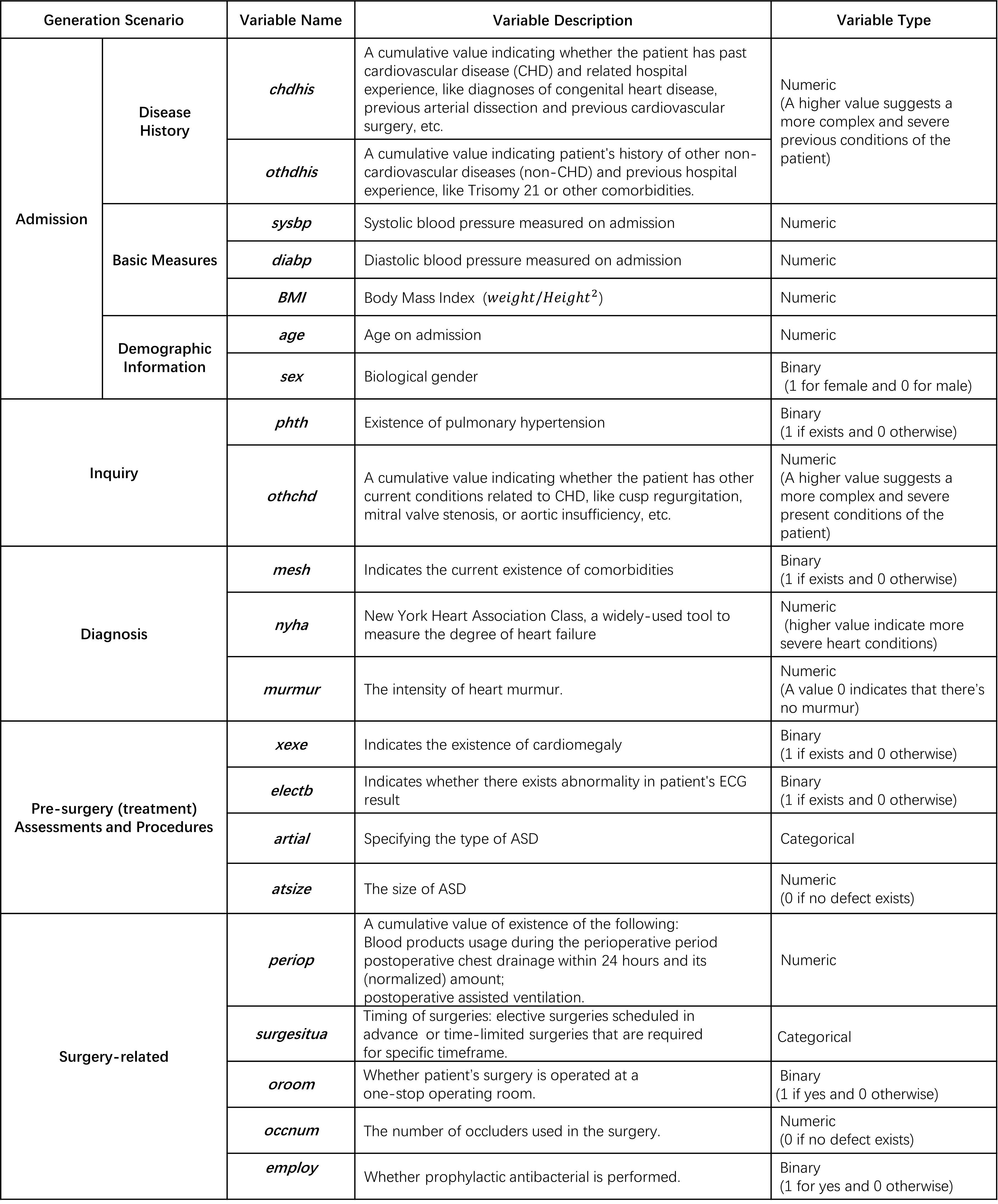
Figure 7: Description of 16 pre-treatment variables and 5 surgery-related variables.

5 Real-world data analysis

In this section, we apply the CRL workflow on an atrial septal defect (ASD) data to demonstrate its usage and performance on real-world observational data. ASD is a birth defect of the heart in which there is a hole in the wall (septum) that divides the upper chambers (atria) of the heart. As a common type of congenital heart disease, ASD has a prevalence of 2.5 out of 1000 in live births and 25% to 30% present in adulthood (Brida et al., 2021; van der Linde et al., 2011).

In this study, we focus on two common ASD treatments: percutaneous interventional closure (PIC) and minimally invasive surgical closure (MISC). PIC involves using catheters to reach the heart through blood vessels and repair the defect with occluder while MISC involves making a small incision in the chest, allowing access to the heart for patching. Specifially, we investigate the HTE of PIC versus MISC (negative treatment) on hospital-free days within one year after discharge (HFD1Y). Hospital-free days are the days patient spent outside of the hospital. Instead of survival or alive days that overemphasize the survival goal, it is more pragmatic and patient-centered, reflecting more information of patient’s quality of life (Auriemma et al., 2021).

In what follows, we first briefly introduce the ASD data. Then we list a few performance metrics designed particularly for HTE estimation in real-world scenario where the ground truth of the treatment effect is not known. Finally, we show the details of CRL application on the ASD data and compare its performance with other baseline models. We also give an example set of rules (See Table 5) learned from CRL and briefly interpret these rules with domain knowledge.

5.1 Overview of the ASD data

The ASD data used in this study is extracted from a congenital heart disease data collected from thirteen clinical centers in China with the initiative to analyze and compare clinical pathways for first-surgery patients (patients undergoing surgery for the first time). The data includes 6780 patient records with 250 variables generated from hospital admission, preoperative examination, diagnoses, all the way to surgery, discharge, and follow-up visit. To implement our analysis, we extract the records of patients that were diagnosed with only ASD and treated with either PIC or MISC. There are only a few missing values in these records, so we simply impute the data with K-Nearest Neighbor (number of neighbors set to 10). The final data includes 2850 observations, with 16 pre-treatment variables and five surgery-related variables, some of which are manually integrated with multiple original variables to make the variable set more concise. Pre-treatment variables include the information generated on admission, through the inquiry and diagnosis, and from pre-surgery medical check results. For instance, on admission, we have: i) two cumulative scores on disease history chdhis and othdhis. If a patient’s chdhis$=3$, it means that the patient has three previous cardiovascular conditions, ii) basic measurements with sysbp and diabp representing systolic and diastolic blood pressure respectively, and BMI the Body Mass Index, and iii) demographic information like age and sex. We give details of all variables in Figure 7, with descriptive statistics in Table LABEL:tab:des.stat.realdata1 for pre-treatment variables and Table 3 for surgery-related variables and outcome HFD1Y.

Table 2: Descriptive statistics of 16 pre-treatment variables.

Covariates	Level	PIC (positive)	MISC (negative)	$p$-value	SMD
		N=2201	N=379
othdhis (%)	0	2154 (97.9)	373(98.4)	0.757	0.077
	1	41(1.9)	6(1.6)
	2	5(0.2)	0(0.0)
	3	1(0.0)	0(0.0)
chdhis(%)	0	13(0.6)	1(0.3)	0.498	0.106
	1	1032(46.9)	195(51.5)
	2	1147(52.1)	182(48.0)
	3	8(0.4)	1(0.3)
	4	1 (0.0)	0 (0.0)
othchd (%)	0	787 (35.8)	147 (38.8)	0.002	0.221
	1	4 (0.2)	2 (0.5)
	2	25 (1.1)	2 (0.5)
	3	2 (0.1)	0 (0.0)
	4	13 (0.6)	9 (2.4)
	5	1311 (59.6)	210 (55.4)
	6	57 (2.6)	7 (1.8)
	7	1 (0.0)	2 (0.5)
	8	1 (0.0)	0 (0.0)
atrial (%)	0	45 (2.0)	4 (1.1)	0.011	0.221
	1	241 (11.0)	33 (8.7)
	2	1861 (84.6)	340 (89.9)
	3	52 (2.4)	1 (0.3)
nyha (%)	1	636 (29.0)	261 (68.9)	$<$0.001	0.92
	2	1491 (67.9)	100 (26.4)
	3	68 (3.1)	18 (4.7)
mesh (%)	0	2071 (94.1)	318 (83.9)	$<$0.001	0.33
	1	130 (5.9)	61 (16.1)
phth (%)	0	2092 (95.0)	310 (81.8)	$<$0.001	0.423
	1	109 (5.0)	69 (18.2)
murmur (%)	0	568 (25.8)	145 (38.3)	$<$0.001	0.341
	1	33 (1.5)	11 (2.9)
	2	302 (13.7)	61 (16.1)
	3	1298 (59.0)	162 (42.7)
electb (%)	0	1401 (63.7)	108 (28.5)	$<$0.001	0.754
	1	800 (36.3)	271 (71.5)
xece (%)	0	1130 (51.3)	311 (82.1)	$<$0.001	0.689
	1	1071 (48.7)	68 (17.9)
sex (%)	0	985 (44.8)	148 (39.1)	0.044	0.116
	1	1216 (55.2)	231 (60.9)
atsize0 (mean (SD))		9.41 (6.39)	17.31 (8.61)	$<$0.001	1.042
sysbp (mean (SD))		203.04 (13.33)	99.58 (12.07)	$<$0.001	0.272
diabp (mean (SD))		63.75 (10.32)	62.05 (10.68)	0.004	0.162
age (mean (SD))		10.26 (9.77)	8.74 (10.26)	0.006	0.152
BMI (mean (SD))		17.54 (5.1)	16.44 (3.60)	0.001	0.248

Due to a significant difference in sample sizes and unsatisfactory overlap between the two treatment groups, we do a propensity score matching (PSM) before CRL application to ensure the satisfaction of three assumptions of potential outcome framework (Zhao et al., 2021) and use the matched data to fit all models for performance evaluation. Details of the matching process can be found in C, after which 26 observations are eliminated from the data and variable atsize0 is replaced by its square root, sq.atsize0 for better covariate balance.

5.2 Performance metrics for real-world observational data

When estimating treatment effect using real-world data, the ground truth is never known. Thus we can no longer use the performance metrics defined for simulated data. Instead, we have to do so in some indirect ways based on what we know, like the following shown:

i) ITE estimation: ITE-based prediction accuracy. It is reasonable to evaluate the potential accuracy of ITE estimation based on the prediction accuracy of known observed outcomes $Y$. Consider $Y{(-1)}=f(X)$ which merely reflects the baseline effect and $Y{(1)}=Y{(-1)}+\tau(X)$. Then for the same outcome prediction model $\hat{Y}=g(\hat{\tau}(x),x)$ using entirely the same variables $x$ but different ITE estimates $\hat{\tau}(x)$, the source of difference in prediction accuracy, say $MSE(g(\hat{\tau}(x))$ mainly comes from the difference in $\hat{\tau}(x)$. Hence in general the method that predicts the outcome better (lower MSE) estimates $\tau(x)$ better.

ii) For treatment recommendation: Empirical expected outcome (EEO). This metric is defined in Qi et al. (2018) as:

$$\hat{V}(d)=\frac{\mathbf{E}_{n}[Y1(A=d(X))/\pi(A,X)]}{\mathbf{E}_{n}[1(A=d(X))/\pi(A,X)]},$$

where $\mathbf{E}_{n}$ denotes empirical average and $d(X)$ denotes a specific personalized treatment strategy that maps a given $X$ to a certain treatment. This metric in essence measures the mean magnitude of $Y$ a treatment strategy is able to achieve when its recommendation of treatments is in line with samples’ actual received treatments. The higher this expected outcome, the better the treatment strategy is, and implicitly, the more accurate our ITE estimation is.

iii) For subgroup identification: Treatment efficient frontier. This metric is proposed in Wang and Rudin (2022) as a graphic comparison of subgroups obtained from different methods given that the identified subgroups differ in group size (proportion of samples) and CATE. Though not always the case, a small group usually has higher CATE than a bigger one, so it is hard to tell which subgroup is better. To balance the trade-off between subgroup size and subgroup CATE, the authors define the concept of treatment efficient frontier which is formed with all dominant groups (subgroup that has no any other subgroup surpasses it in both size and CATE) a certain method identifies. This frontier is then mapped to the two-dimensional coordinate system with the $x$-axis being the size and $y$-axis the CATE estimates of the dominant groups. See Figure 8 for example. With this graph, we can see how quickly the estimated treatment effect magnitude decays as the subgroup covers more samples and easily spot the method that has the highest frontier since they find subgroups with larger size and CATE.

Table 3: Descriptive statistics of five surgery-related variables and outcome variable HFD1Y.

Vairables	PIC (positive)	MISC (negative)	$p$-value	SMD
(mean (SD))	N=2201	N=379
surgesitua	1.00 (0.06)	1.01 (0.09)	0.171	0.064
oroom	0.22 (0.42)	0.31 (0.46)	$<$0.001	0.207
occnum	1.00 (0.13)	0.10 (0.30)	$<$0.001	3.858
periop	1.12 (0.37)	3.09 (0.82)	$<$0.001	3.111
employ	0.64 (0.48)	0.70 (0.46)	0.016	0.136
HFD1Y	360.05 (4.75)	352.49 (6.17)	$<$0.001	1.373

5.3 Model implementation

Considering the above performance metrics, especially the ITE-based prediction accuracy, we implement all methods (CRL and other baseline methods) with the following procedure:

We first split the ASD data into three parts: 40% (estimation set) for ITE estimation with all methods; 40% (prediction set) for outcome prediction using the least squares model (or any other proper prediction models) fed with all same variables except the different ITE estimated by different methods in the previous step. The remaining 20% data (test set) is used to report the first two performance metrics, i.e., $MSE(g(\hat{\tau}(x))$ and EEO.

We repeat the above procedure 100 times with randomly re-sampled ASD data and tune the parameters of models with the same logic as we do in the simulation part. See B for details.

To evaluate treatment efficient frontier, we use the entire data to fit all models for each of the re-sampled data, since CRL generally needs more observations to discover potential subgroups. For each method to be compared, we pool the subgroups identified from all 100 repetitions together and find its dominant subgroups which form the ultimate frontier.

5.4 Model results and interpretation

We list the MSE of the predicted HFD1Y and EEO of all methods averaged over 100 repetition in the first and second row in Table 4. It is obvious that all methods yield similar accuracies of outcome prediction, implying that they perform similarly in estimating ITE. Therefore, the EEO based on the estimated ITE is also pretty close. Figure 8 shows the treatment efficient frontier of all methods. Obviously, CRL identifies subgroups with a variety of sizes, ranging from 0.1 to 0.85, yet the other two methods, especially OWE, only focuses on big subgroups with relatively small subgroup CATE. Note that we do not show the frontier of Causal Forestin this figure as it overlaps with the frontier of CRL whose dominant groups are part of Causal Forestgroups.

The above results demonstrate that CRL achieves at least comparable results against baseline methods in terms of ITE estimation, treatment recommendation and subgroup identification on the ASD data. Moreover, it provides us enhanced understanding of ITE of ASD treatments on HFD1Y through the contributing informative rules we learned from the whole workflow.

Table 4: Mean squared error (MSE) and empirical expected outcome (EEO) averaged on 100 repetitions of ASD data applying CRL and other baseline models. SD is the standard deviation of MSE and EEO.

	CRL	CF	OWE	PRIM
Mean MSE (SD)	21.710 (14.554)	21.765 (14.577)	21.768 (14.583)	21.622 (14.541)
Mean EEO (SD)	359.621 (0.330)	359.691 (0.323)	359.353 (0.588)	359.691 (0.323)

For a concise presentation of what we learned from the ASD data with CRL, we list the eight rules that impact the estimated treatment effect the most in a randomly chosen rule set out of the 100 rule sets, with their corresponding CATE estimates and learned weights (See Table 5). The rules are displayed in decreasing order of the absolute value of the subgroup CATE multiplied by the subgroup weight and the signed product is shown, indicating the effect direction and magnitude of each rule. For example, the first rule means that when a patient with abnormal ECG result, BMI$>$14.4, othchd$>$0 and is operated at a one-stop operating room, the patient’s ITE of PIC against MISC will increase by 349.44 days. However, this estimate will then decrease by 323.34 if the patient’s age is between five and nine. The final ITE estimate of a patient is the summation of all the products corresponding to the subgroups a patient belongs to, showing how a patient’s ITE is affected by the combination of potential rules.

These eight rules identify several important factors (with meaningful cut-off values like $14.44$ for BMI) of treatment effect of PIC against MISC on HFD1Y, such as age, BMI, electb, oroom and nyha. Age and BMI are the two most involved factors in the rules, indicating they play indispensable roles in the way HFD1Y is affected by PIC and MISC. This is consistent with Hughes et al. (2002) and Qi et al. (2020) stating that age and weight-related factors like BMI are particularly important in surgery decision and the prognosis of ASD such as length of hospital stay. Compared to MISC, PIC in general has an advantage of shorter hospital stay and is more suitable for non-underweight children or older children (Qi et al., 2020), which is reflected with the HFD1Y increase in the first (BMI $>$ 14.44) and second rule (age$>$8). For children aged between five and nine (second rule), the decrease of HFD1Y, or the increase of hospital stay may be due to a lower percentage of PIC treated patients within the group compared to that of the remaining population (81% versus 85%). This reveals the preference for MISC against PIC in young-aged group, which has been a fact in past ASD treatment parctice (Karamlou et al., 2008).

In addition, these rules identify multiple cut-off values for the same factors, such as age with thresholds at 8 (third rule) and 15 (seventh rule), together with nyha and sq.atsize0, revealing potential complex interactions between these factors. Although there is little evidence on these interactions, we believe they enlighten people in the community on new research directions such as designing rigorous experiment to further validate these underlying relationships.

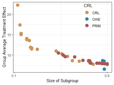
Figure 8: Treatment efficient frontiers of all methods fit for 100 repititions.

Table 5: Eight subgroups that most impact the estimates of treatment effect, displayed in descending order of the absolute value of the subgroup CATE multiplied by the subgroup weight.

subgroup	CATE	Weight	CATE $\times$ Weight
BMI$>$14.44 and electb=1 and oroom=1 and othchd$>$0	2.92	119.54	349.44
age$\leq$9 and age$>$5	7.62	$-42.42$	$-323.34$
age$>$8 and nyha$\leq$1	5.98	50.70	303.11
age$>$7 and nyha$\leq$1 and sq.atsize0$\leq$4.8	7.09	$-42.64$	$-302.33$
murmur$\leq$2 and sysbp$>$100.35	7.79	$-31.14$	$-242.45$
age$>$5 and BMI$>$17.17 and electb=1	6.09	$-38.38$	$-233.79$
age$>$15 and BMI$>$13.7	6.85	$-33.52$	$-229.63$
diabp$>$59 and electb=1 and oroom=0	6.80	29.20	198.66

6 Conclusions and future work

This study introduces a rule-based framework, CRL, aimed at enhancing our understanding of HTE in industries like healthcare. Drawing inspiration from the PDR framework for interpretablility in machine learning, CRL enables a high-level interpretability in HTE estimation through the entire workflow on identifying relevant informative rules. The CRL leverages causal forest to discover a pool of potential rules for ITE estimation (rule discovery) and then utilizes D-learning method to filter out non-informative rules, imposing sparisty on the rules (rule selection) . By deconstructing the estimated ITE through a weighted combination of the informative rules selected by D-learning, CRL explores HTE with a novel perspective, i.e., the relationship between group level and individual level treatment effect. Through understandable rules themselves, their corresponding CATE estimates and weights in the combination, the model-based interpretability is increased. We also introduce a comprehensive procedure for evaluating each causal rule from multiple perspectives (rule analysis), offering post-hoc interpretability to the identified subgroups. The remaining rules which survive in post-hoc analysis may reveal potential meaningful interactions between involved vriables, paving the way for further investigation and validation. The applications of CRL with both the simulated RCT data sets and the real-world observational data demonstrate the power of CRL in ITE estimation accuracy and HTE interpretablility.

Overall, our study enriches the toolkit for estimating HTE through an interpretable rule-based approach which contributes to the fields of heterogeneous treatment effect estimation, subgroup identification, and optimal policy learning.

This research has several limitations in methodology that could be improved in later studies. First of all, CRL requires the outcome of interest must be a continuous and positive measure which prefers higher values. Treatment in our study is also limited to the binary case. These limits greatly hinder the wide application of the method in practice. Secondly, our assumption of ITE is based on a linear combination of potential rules while the non-linear case is not discussed. Thirdly, the selected potential subgroups and their weights are actually determined by the entire population instead of subgroup population in the D-learning process. Thus CRL cannot deal with scenarios where rules have to be customized for different subgroups. Last but not least, in the evaluation of CRL from policy learning perspective, we simply recommend treatments based on the sign of the estimated ITE and do not consider the cost-sensitive scenarios where treatment resource are constrained. Future work may introduce more economic factors and discuss how to better estimate treatment effect and recommend treatment in such complex situations.

Appendix A Three assumptions of Neyman–Rubin potential outcome framework

We list the three basic assumptions of the potential outcome framework below: 1. Stable Unit Treatment Value Assumption (SUVTA): The potential outcomes of any instance do not vary with the treatments assigned to other instances and there is only one version of each treatment. 2. Ignorability/Unconfoundedness: Treatment assignment is independent of the potential outcomes conditional on the observed covariates, i.e., $A\perp\{Y(1),Y(-1)\}|X=x$. This assumption implies there are no other unmeasured confounding factors and treatment assignment can be considered as random given the covariates $X$.

Rosenbaum and Rubin (1983) gives an equivalent assumption conditioned on the propensity score, i.e., $A\perp\{Y(1),Y(-1)\}|\pi(a,x)$, which is especially useful in high-dimension settings where it is difficult to match samples with the original covariates. Our method is based on this assumption. 3. Positivity/Overlap: $0<Pr(A=1|X=x)<1$, i.e., any instance has a positive probability of receiving either treatment given $X=x$. This assumption ensures the existence of samples for both treatment groups so that it is possible to estimate the treatment effect.

Appendix B Parameters tuning for CRL

This part lists several parameters need to be tuned when fitting CRL.

In the rule discovery phase, we tune the parameters of CRL inherited from Causal Forest, such as num.trees specifying the number of trees in the forest, min.node.size the minimum sample number of observations in each tree leaf, and mtry the number of variables tried for each split when fitting the forest. Other parameters of causal forest include honesty.fraction and sample.fraction specifying the sample allocation proportion in honest estimation and sample splitting respectively. In the rule selection phase, the main parameter is $\lambda$ that controls the degree of penalty in Equation (6). We show below the details of tuning the above parameters for simulated data and real-world data respectively.

B.0.1 Parameters tuning of CRL for simulated data

Since we only have nine covariates in our simulated data, mtry is arbitrarily set to be nine in all data sets to increase the likelihood of various combination of covariates in rules. honesty.fraction and sample.fraction are set to the default values.

We adopt a greedy goal in tuning other parameters. Instead of optimizing only one performance metric, we consider finding the best parameters which simultaneously achieve these three metrics: minimum MSE, largest population overlap, and largest number of true rules identified. Empirically, we find that 200 trees are sufficient to give satisfying results given a varying combination of other parameters, thus we set num.trees to 200 in all data sets to save computation cost and avoid too many fake rules. min.node.size appears to be the most sensitive parameter since it determines how many samples from both treatments are used to estimate the treatment effect. This parameter is mainly affected by the number of observations to fit causal forest and merely affected by the true number of positive subgroups and effect size. So we simply focus the tuning of this parameter for data sets with $N=5000$ and $N=10,000$.

For a given number of observations, we have data sets with varying effect sizes and true numbers of positive subgroups. We do a 10-fold cross validation on each data set. Based on our tuning results, most of the time, there is always one set of parameters that is able to optimize all three metrics for all the data sets. However, this is not theoretically guaranteed because sometimes a setting with the largest number of true rules does not bring the minimum MSE or the largest population overlap. Fortunately, we found that in this case, the MSE and population overlap have similar values for comparable settings. Thus, we give our first priority to number of true rules, and second and third priorities to MSE and population overlap. We find that the overall best min.node.size is 50 and 100 respectively for data sets with 5000 and 10,000 observations. We tune $\lambda$ with 100 values between 0.0004 and 4 with an interval of 0.04 with 10-fold cross validation and the one that gives the minimum mean error is chosen. The ranges of parameter values we tested are summarized in Table 6.

Table 6: Summary of parameters tuning for CRL applied on simulated data.

Parameters	Tuning Range	Final value chosen
num.trees	(100,200,300,400,	200
	500,1000,1500,2000)
mtry	-	Nine
min.node.size
(N = 5,000)	(20,30,40,50,60,70,80)	50
(N = 10,000)	(50,60,70,80,90,100,110,120,130)	100
$\lambda$	100 values in [0.0004,4]	The one that gives the
	with an interval of 0.04	minimum mean error in
		10-fold cross validation

B.0.2 Parameters tuning of CRL for ASD data

Given the number of observations around 2,500, the optimized num.trees is still 200 and the min.node.size is 20 to achieve a good balance of similar greedy objectives: high ITE-based prediction accuracy, bigger empirical expected outcome, and higher treatment efficient frontier.

Appendix C Propensity score matching of the ASD data

We use R package MatchIt (Ho et al., 2011) to implement the whole PSM procedure on the pre-treatment variables of the ASD data. Note that we recode the negative treatment to $0$ instead of $-1$. The procedure involves three core aspects: propensity score estimation, data matching, and balance diagnostics. We measure the distance between samples in terms of propensity scores and try various combinations of propensity score estimation models and matching methods. Our final choice goes to a covariate balancing propensity score (CBPS) (Imai and Ratkovic, 2014) model with the following implementation formula to estimate propensity scores, by which the samples are stratified into subclasses for matching:

treatment = othdhis + chdhis + othchd + atrial + $\sqrt{atsize0}$ + nyha + mesh + phth + murmur + electb + xece + sysbp + diabp + age + sex + BMI + employ.

This combination is able to achieve i) good overlap within each subclass, see Figure 9(b). The improvement of overlap before (Figure 9(a)) and after (Figure 9(b)) the matching is obvious; ii) balanced covariates between two treatment groups. Before the matching, there are only five variables that are considered balanced between the two groups, having a standardized mean difference (SMD) within 10%. After the matching, all covariates are balanced other than the square root of atsize0 (sq.atsize0), whose SMD value is slightly above the threshold (0.1005). Here, we consider this difference to be acceptable as it is what we can best achieve from all attempts. See the love plot in Figure 9(c) for the comparison of covariates balance between treatments before and after the matching; iii) least observations discarded. The matching process retain a total of 2554 observations with 2180 for positive treatment PIC and 374 for negative treatment MISC. We then apply CRL on this matched data set.

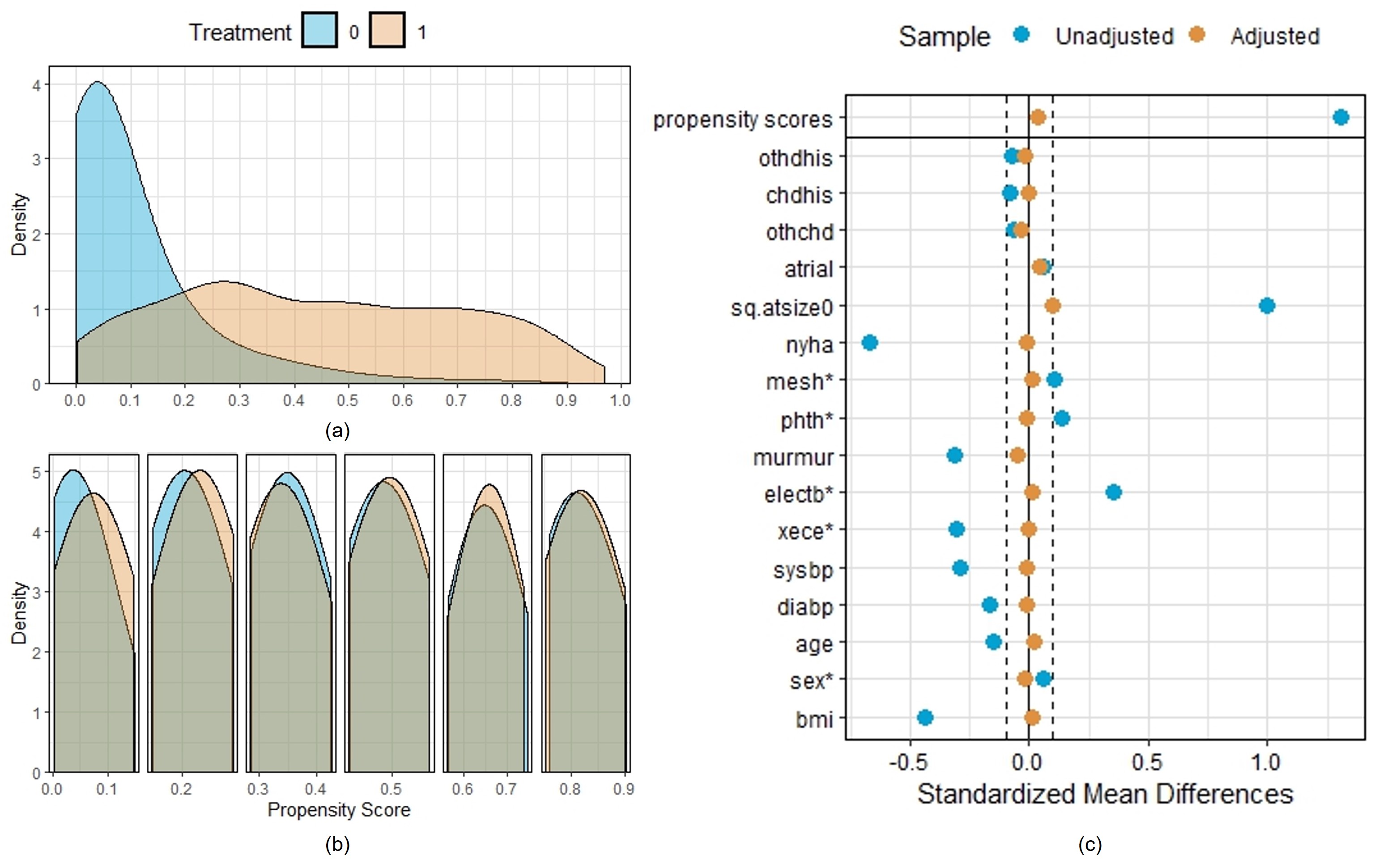
Figure 9: Detials of propensity score matching on the ASD data, including density of propensity scores before (a) and after (b) matching and love plot (c) of both treatment groups.

References

- Alaa and Schaar (2018) Alaa, A., Schaar, M., 2018. Limits of estimating heterogeneous treatment effects: Guidelines for practical algorithm design, in: International Conference on Machine Learning, PMLR. pp. 129–138.
- Alaa et al. (2017) Alaa, A.M., Weisz, M., van der Schaar, M., 2017. Deep counterfactual networks with propensity-dropout. arXiv preprint arXiv:1706.05966 .
- Athey and Imbens (2016) Athey, S., Imbens, G., 2016. Recursive partitioning for heterogeneous causal effects. Proceedings of the National Academy of Sciences 113, 7353–7360.
- Athey et al. (2019) Athey, S., Tibshirani, J., Wager, S., 2019. Generalized random forests. The Annals of Statistics 47, 1148–1178. URL: https://doi.org/10.1214/18-AOS1709, doi:10.1214/18-AOS1709.
- Auriemma et al. (2021) Auriemma, C.L., Taylor, S.P., Harhay, M.O., Courtright, K.R., Halpern, S.D., 2021. Hospital-free days: A pragmatic and patient-centered outcome for trials among critically and seriously ill patients. American Journal of Respiratory and Critical Care Medicine 204, 902–909.
- Bargagli-Stoffi et al. (2023) Bargagli-Stoffi, F.J., Cadei, R., Lee, K., Dominici, F., 2023. Causal rule ensemble: Interpretable discovery and inference of heterogeneous treatment effects. arXiv:2009.09036.
- Berger and Zhou (2014) Berger, V.W., Zhou, Y., 2014. Kolmogorov–smirnov test: Overview. Wiley Statsref: Statistics Reference Online .
- Breitmar et al. (2023) Breitmar, N.A., Harding, M., Lamarche, C., 2023. Using grouped data to estimate revenue heterogeneity in online advertising auctions, in: AEA Papers and Proceedings, American Economic Association 2014 Broadway, Suite 305, Nashville, TN 37203. pp. 161–165.
- Brida et al. (2021) Brida, M., Chessa, M., Celermajer, D., Li, W., Geva, T., Khairy, P., Griselli, M., Baumgartner, H., Gatzoulis, M.A., 2021. Atrial septal defect in adulthood: a new paradigm for congenital heart disease. European Heart Journal 43, 2660–2671. doi:10.1093/eurheartj/ehab646.
- Brida and Gatzoulis (2020) Brida, M., Gatzoulis, M.A., 2020. Adult congenital heart disease: Past, present, future. International Journal of Cardiology Congenital Heart Disease 1, 100052.
- Cattaneo et al. (2022) Cattaneo, M.D., Chandak, R., Klusowski, J.M., 2022. Convergence rates of oblique regression trees for flexible function libraries. arXiv preprint arXiv:2210.14429 .
- Chen et al. (2015) Chen, G., Zhong, H., Belousov, A., Devanarayan, V., 2015. A PRIM approach to predictive-signature development for patient stratification. Statistics in Medicine 34, 317–342.
- Chen et al. (2017) Chen, S., Tian, L., Cai, T., Yu, M., 2017. A general statistical framework for subgroup identification and comparative treatment scoring. Biometrics 73, 1199–1209.
- Chen et al. (2023) Chen, Y., Calabrese, R., Martin-Barragan, B., 2023. Interpretable machine learning for imbalanced credit scoring datasets. European Journal of Operational Research 312, 357–372.
- Chernozhukov et al. (2018) Chernozhukov, V., Chetverikov, D., Demirer, M., Duflo, E., Hansen, C., Newey, W., Robins, J., 2018. Double/debiased machine learning for treatment and structural parameters.
- Cintron et al. (2022) Cintron, D.W., Adler, N.E., Gottlieb, L.M., Hagan, E., Tan, M.L., Vlahov, D., Glymour, M.M., Matthay, E.C., 2022. Heterogeneous treatment effects in social policy studies: an assessment of contemporary articles in the health and social sciences. Annals of Epidemiology 70, 79–88.
- Cintron et al. (2023) Cintron, D.W., Gottlieb, L.M., Hagan, E., Tan, M.L., Vlahov, D., Glymour, M.M., Matthay, E.C., 2023. A quantitative assessment of the frequency and magnitude of heterogeneous treatment effects in studies of the health effects of social policies. SSM-Population Health 22, 101352.
- Cui et al. (2023) Cui, Y., Kosorok, M.R., Sverdrup, E., Wager, S., Zhu, R., 2023. Estimating heterogeneous treatment effects with right-censored data via causal survival forests. Journal of the Royal Statistical Society Series B: Statistical Methodology 85, 179–211.
- Dwivedi et al. (2020) Dwivedi, R., Tan, Y.S., Park, B., Wei, M., Horgan, K., Madigan, D., Yu, B., 2020. Stable discovery of interpretable subgroups via calibration in causal studies. International Statistical Review 88, S135–S178.
- Foster et al. (2011) Foster, J.C., Taylor, J.M., Ruberg, S.J., 2011. Subgroup identification from randomized clinical trial data. Statistics in Medicine 30, 2867–2880.
- Friedman and Popescu (2008) Friedman, J., Popescu, B., 2008. Predictive learning via rule ensembles. The Annals of Applied Statistics 2, 916–954. doi:10.1214/07-AOAS148.
- Friedman and Fisher (1999) Friedman, J.H., Fisher, N.I., 1999. Bump hunting in high-dimensional data. Statistics and Computing 9, 123–143.
- Garcia et al. (2023) Garcia, G.G.P., Steimle, L.N., Marrero, W.J., Sussman, J.B., 2023. Interpretable policies and the price of interpretability in hypertension treatment planning. Manufacturing & Service Operations Management in press.
- Gong and Liu (2023) Gong, J., Liu, S., 2023. Partially observable collaborative model for optimizing personalized treatment selection. European Journal of Operational Research 309, 1409–1419.
- Green and Kern (2012) Green, D.P., Kern, H.L., 2012. Modeling heterogeneous treatment effects in survey experiments with bayesian additive regression trees. Public Opinion Quarterly 76, 491–511.
- He et al. (2022) He, Y., Huang, G., Chen, S., Teng, J., Wang, K., Yin, Z., Sheng, L., Liu, Z., Qiao, Y., Shao, J., 2022. X-learner: Learning cross sources and tasks for universal visual representation, in: Computer Vision–ECCV 2022: 17th European Conference, Tel Aviv, Israel, October 23–27, 2022, Proceedings, Part XXVI, Springer. pp. 509–528.
- Herlitz (2017) Herlitz, A., 2017. Comparativism and the grounds for person-centered care and shared decision making. The Journal of Clinical Ethics 28, 269–278.
- Ho et al. (2011) Ho, D.E., Imai, K., King, G., Stuart, E.A., 2011. MatchIt: Nonparametric preprocessing for parametric causal inference. Journal of Statistical Software 42, 1–28. doi:10.18637/jss.v042.i08.
- Huang et al. (2017a) Huang, X., Sun, Y., Chatterjee, S., 2017a. SubgrpID: Patient Subgroup Identification for Clinical Drug Development. URL: https://CRAN.R-project.org/package=SubgrpID. r package version 0.10.
- Huang et al. (2017b) Huang, X., Sun, Y., Trow, P., Chatterjee, S., Chakravartty, A., Tian, L., Devanarayan, V., 2017b. Patient subgroup identification for clinical drug development. Statistics in Medicine 36, 1414–1428.
- Hughes et al. (2002) Hughes, M., Maskell, G., Goh, T., Wilkinson, J., 2002. Prospective comparison of costs and short term health outcomes of surgical versus device closure of atrial septal defect in children. Heart 88, 67–70.
- Huling and Yu (2021) Huling, J.D., Yu, M., 2021. Subgroup identification using the personalized package. Journal of Statistical Software 98, 1–60. doi:10.18637/jss.v098.i05.
- Imai and Ratkovic (2014) Imai, K., Ratkovic, M., 2014. Covariate balancing propensity score. Journal of the Royal Statistical Society Series B: Statistical Methodology 76, 243–263.
- Johansson et al. (2016) Johansson, F., Shalit, U., Sontag, D., 2016. Learning representations for counterfactual inference, in: International Conference on Machine Learning, PMLR. pp. 3020–3029.
- Karamlou et al. (2008) Karamlou, T., Diggs, B.S., Ungerleider, R.M., McCrindle, B.W., Welke, K.F., 2008. The rush to atrial septal defect closure: is the introduction of percutaneous closure driving utilization? The Annals of thoracic surgery 86, 1584–1591.
- Kraus et al. (2023) Kraus, M., Tschernutter, D., Weinzierl, S., Zschech, P., 2023. Interpretable generalized additive neural networks. European Journal of Operational Research in press.
- Krieger and Valente (2014) Krieger, E.V., Valente, A.M., 2014. Heart failure treatment in adults with congenital heart disease: Where do we stand in 2014? Heart 100, 1329–1334.
- van der Laan and Rose (2011) van der Laan, M.J., Rose, S., 2011. Targeted Learning: Causal Inference for Observational and Experimental Data. Springer.
- Laber and Zhao (2015) Laber, E.B., Zhao, Y.Q., 2015. Tree-based methods for individualized treatment regimes. Biometrika 102, 501–514.
- van der Linde et al. (2011) van der Linde, D., Konings, E.E., Slager, M.A., Witsenburg, M., Helbing, W.A., Takkenberg, J.J., Roos-Hesselink, J.W., 2011. Birth prevalence of congenital heart disease worldwide: A systematic review and meta-analysis. Journal of the American College of Cardiology 58, 2241–2247. doi:https://doi.org/10.1016/j..2011.08.025.
- Lipkovich et al. (2011) Lipkovich, I., Dmitrienko, A., Denne, J., Enas, G., 2011. Subgroup identification based on differential effect search—a recursive partitioning method for establishing response to treatment in patient subpopulations. Statistics in Medicine 30, 2601–2621.
- Loh (2011) Loh, W.Y., 2011. Classification and regression trees. Wiley Interdisciplinary Reviews: Data Mining and Knowledge Discovery 1, 14–23.
- Loh et al. (2019) Loh, W.Y., Cao, L., Zhou, P., 2019. Subgroup identification for precision medicine: A comparative review of 13 methods. Wiley Interdisciplinary Reviews: Data Mining and Knowledge Discovery 9, e1326.
- Lunceford and Davidian (2004) Lunceford, J.K., Davidian, M., 2004. Stratification and weighting via the propensity score in estimation of causal treatment effects: a comparative study. Statistics in Medicine 23, 2937–2960.
- Murdoch et al. (2019) Murdoch, W.J., Singh, C., Kumbier, K., Abbasi-Asl, R., Yu, B., 2019. Definitions, methods, and applications in interpretable machine learning. Proceedings of the National Academy of Sciences 116, 22071–22080. doi:10.1073/pnas.1900654116.
- Murphy (2003) Murphy, S.A., 2003. Optimal dynamic treatment regimes. Journal of the Royal Statistical Society: Series B (Statistical Methodology) 65, 331–355.
- Polley et al. (2011) Polley, E., Rose, S., Laan, M., 2011. Super Learning. chapter 3. pp. 43–66. doi:10.1007/978-1-4419-9782-1_3.
- Qi et al. (2020) Qi, H., Zhao, J., Tang, X., Wang, X., Chen, N., Lv, W., Bian, H., Wang, S., Yuan, B., 2020. Open heart surgery or echocardiographic transthoracic or percutaneous closure in secundum atrial septal defect: a developing approach in one chinese hospital. Journal of Cardiothoracic Surgery 15, 1–6.
- Qi et al. (2018) Qi, Z., Liu, Y., et al., 2018. D-learning to estimate optimal individual treatment rules. Electronic Journal of Statistics 12, 3601–3638.
- Qian and Murphy (2011) Qian, M., Murphy, S.A., 2011. Performance guarantees for individualized treatment rules. Annals of Statistics 39, 1180–1210.
- R Core Team (2021) R Core Team, 2021. R: A Language and Environment for Statistical Computing. R Foundation for Statistical Computing. Vienna, Austria. URL: https://www.R-project.org/.