Near-Optimality of Finite-Memory Codes and Reinforcement Learning for Zero-Delay Coding of Markov Sources

Abstract

We study the problem of zero-delay coding of a Markov source over a noisy channel with feedback. We first formulate the problem as a Markov decision process (MDP) where the state is a previous belief term along with a finite memory of channel outputs and quantizers. We then approximate this state by marginalizing over all possible beliefs, so that our policies only use the finite-memory term to encode the source. Under an appropriate notion of predictor stability, we show that such policies are near-optimal for the zero-delay coding problem as the memory length increases. We also give sufficient conditions for predictor stability to hold, and propose a reinforcement learning algorithm to compute near-optimal finite-memory policies. These theoretical results are supported by simulations.

I Introduction

The zero-delay coding problem involves compressing and transmitting an information source over a noisy channel with feedback and without delay, while minimizing the expected distortion at the receiver. This zero-delay restriction is of practical relevance in many applications, including live-streaming and real-time sensor networks. However, this restriction means that classical Shannon-theoretic methods, with results generally asymptotic in nature, are not viable.

There has been success in studying this problem using stochastic control techniques. In particular, [1, 2] consider finite alphabets and finite time horizons and show optimality of restricted classes of policies. Similar optimality and existence results are presented for infinite time horizons in [3] (with feedback) and [4] (without feedback). The continuous-alphabet, infinite-horizon case is studied in [5]. However, these stochastic control techniques often utilize a state that is probability measure-valued (such a state is often called the “predictor” in the literature). This state space is computationally difficult to work with, and thus actually obtaining effective coding schemes for a given zero-delay coding problem is still an open problem.

There has been much recent work on learning-theoretic methods in stochastic control for very general state and action spaces. In particular, approximation techniques leading to near-optimal solutions are well-suited to setups such as the zero-delay coding problem, where exact methods are intractable. Some of these techniques use quantization schemes to approximate the underlying state space; for example, refer to [6, 7] and related reinforcement learning algorithms in [8, 9]. While these quantization-based methods can be used to find near-optimal solutions, the quantization process introduces additional computational complexity, both during learning and implementation. Furthermore, these methods give explicit performance bounds only under certain continuity assumptions which are not applicable in the zero-delay coding problem; for the zero-delay coding problem, the convergence to near-optimality is only asymptotic; see [10] for additional quantization-based approaches and algorithms. We will see that our finite-memory approach, while requiring filter stability conditions, is computationally simpler than these quantization methods.

In order to avoid the computational overhead of quantization, as well as achieve more exact bounds on near-optimality, we will instead build on recent results from [11] which uses a finite history of past observations and control actions. The work in [11] also provides a Q-learning solution to obtain such near-optimal policies, which we will adapt to our setup. This approach relies on filter stability, which is a measure of how quickly a process forgets its prior as it collects observations. Our results will use the related question of predictor stability. Under predictor stability, this finite history acts as a good approximation of the true predictor, leading to explicit performance bounds on the resulting policy for the zero-delay coding problem. Note that filter or predictor stability is typically established in two ways:

• The transition kernel of the underlying state space is in some sense sufficiently ergodic, so that regardless of the observations, the filter/predictor process inherits this ergodicity and forgets its prior over time.

• The observations are in some sense sufficiently informative, so that, regardless of the prior, the filter/predictor process tracks the true state process.

For a detailed review of these filter stability methods in the control-free case, see [12]. However, we will see that in the zero-delay coding problem, the observations depend not only on the noisy channel but also on how we encode the information at the receiver. Most results in the literature assume that the observation kernel is time-invariant, which is not applicable here; so we will prove and use generalized results for when this kernel is control-dependent. In particular, we will generalize recent results from [13], which uses joint properties of the state and observation kernels to obtain exponential filter stability, as well as discuss recent observability-type conditions from [14, 15] and how they may be generalized to obtain predictor stability in our context.

Additional work related to finite-memory policies can be found in [16, 17]. However, [16] does not provide a performance bound based on window length, and [17] still utilizes a nearest-neighbour quantization map. Furthermore, [17] only provides near-optimality of the discounted-cost criteria for discount factors bounded away from one; in the zero-delay coding problem, we are generally interested in taking discount factors very close to one in order to obtain approximations to the average-cost problem.

Contributions

In this paper, we prove near-optimality of finite-memory coding policies for the zero-delay coding problem over a noisy channel with feedback, and explicitly bound the performance of such policies in terms of a predictor stability term. We generalize some existing predictor stability results to the case where the observation kernel is control-dependent, and apply these results to some example zero-delay coding problems. We also discuss a Q-learning algorithm that converges to such a near-optimal policy, and provide supporting simulation results.

II Notation and Preliminaries

Let $\mathbb{X}$ be a finite set and let our information source be a Markov process $(x_{t})_{t\geq 0}$ taking values in $\mathbb{X}$. Let $T(x_{t+1}|x_{t})$ be its transition kernel, which we assume is irreducible and aperiodic, and thus admits a unique invariant measure. Let $x_{0}\sim{\pi_{0}}$ (we will also call ${\pi_{0}}$ the prior). Let $\mathcal{M}$ and $\mathcal{M^{\prime}}$ be the input and output alphabets of the noisy channel, which we assume are finite, and let $(q_{t})_{t\geq 0}$ and $(q^{\prime}_{t})_{t\geq 0}$ be the respective processes. We will denote the channel kernel by $O(q^{\prime}_{t}|q_{t})$, which gives the probability of the channel output being $q^{\prime}_{t}$ given its input is $q_{t}$. Finally, let $\hat{\mathbb{X}}$ be some finite set of reconstruction values, and let $(\hat{x}_{t})_{t\geq 0}$ take values in $\hat{\mathbb{X}}$.

Throughout, given some sequence $(a_{t})_{t\geq 0}$, we will use the notation $a_{[n,k]}\coloneqq(a_{n},a_{n+1},\ldots,a_{k})$ for $n\leq k$. Also, although everything is finite here, for ease of notation as well as providing easier generalizations to uncountable spaces, we will often write sums as integrals over the appropriate measure. For example, rather than writing $\sum_{\mathbb{X}}T(x^{\prime}|x)$ we may write $\int_{\mathbb{X}}T(dx^{\prime}|x)$.

Consider sequences of functions $(\gamma^{e}_{t})_{t\geq 0}$, which we call the encoder policy, and $(\gamma^{d}_{t})_{t\geq 0}$, which we call the decoder policy. In addition to the current source symbol, the encoder has access to all past source symbols and channel inputs, and all past channel outputs in the form of feedback. In addition to the current channel output, the decoder has access to all previous channel outputs. That is, $(\gamma^{e}_{t})_{t\geq 0}$ and $(\gamma^{d}_{t})_{t\geq 0}$ are such that

$$\gamma^{e}_{t}:\mathbb{X}^{t+1}\times\mathcal{M}^{t}\times\left(\mathcal{M^{\prime}}\right)^{t} \to\mathcal{M} \gamma^{d}_{t}:\left(\mathcal{M^{\prime}}\right)^{t+1} \to\hat{\mathbb{X}}$$

$$(x_{[0,t]},q_{[0,t-1]},q^{\prime}_{[0,t-1]}) \mapsto q_{t} q^{\prime}_{[0,t]} \mapsto\hat{x}_{t}.$$

We consider the discounted-cost criterion for the zero-delay coding problem, which is to find encoder and decoder policies such that the following is minimized:

$$J_{\beta}({\pi_{0}},\gamma^{e},\gamma^{d}) \coloneqq\mathbf{E}^{\gamma^{e},\gamma^{d}}_{\pi_{0}}\left[\sum_{t=0}^{\infty}\beta^{t}d(x_{t},\hat{x}_{t})\right],$$ (1)

where $d:\mathbb{X}\times\hat{\mathbb{X}}\to\mathbb{R}_{+}$ is a given distortion function and $\beta\in(0,1)$ is a given discount factor. We use $\mathbf{E}^{\gamma^{e},\gamma^{d}}_{\pi_{0}}$ and $P^{\gamma^{e},\gamma^{d}}_{\pi_{0}}$ to denote expectations (respectively, probabilities) under encoder policy $\gamma^{e}$, decoder policy $\gamma^{d}$, and prior ${\pi_{0}}$. Later, some measures will be independent of the prior and/or the policy adopted, and in these cases we will omit them from the notation.

Note that the discounted-cost criterion is not the standard objective for the zero-delay coding problem; we are usually concerned with the average-cost criterion. However, it can be shown that as $\beta\to 1$, a policy that is near-optimal for the discounted-cost problem is also near-optimal for the average-cost problem [9]. Thus, all of the results in this paper also hold for the average-cost criterion by taking $\beta$ sufficiently close to $1$. Indeed, in our simulations we will take $\beta=0.99$ to obtain an approximation of the average-cost criterion.

Since all our sets are finite, there always exists an optimal decoder policy for a given decoder policy; so without loss of optimality, we can search only for an optimal encoder policy and assume that it is paired with an optimal decoder policy. We will denote such a joint encoder-decoder policy by $\gamma\coloneqq(\gamma^{e},\gamma^{d*})$, where $\gamma^{d*}$ is an optimal decoder policy given $\gamma^{e}$. We denote the infimum of (1) by

$$J^{*}_{\beta}({\pi_{0}}) \coloneqq\inf_{\gamma}J_{\beta}({\pi_{0}},\gamma).$$

For fixed $(x_{[0,t-1]},q_{[0,t-1]},q^{\prime}_{[0,t-1]})$, consider the function $\gamma^{e}(\cdot,x_{[0,t-1]},q_{[0,t-1]},q^{\prime}_{[0,t-1]}):\mathbb{X}\to\mathcal{M}$. Such a function (i.e., a mapping from $\mathbb{X}$ to $\mathcal{M}$) is called a quantizer. We denote the set of all such quantizers by $\mathcal{Q}$. Thus we can view an encoder policy $\gamma^{e}$ as selecting a quantizer $Q_{t}\in\mathcal{Q}$ based on the information $(x_{[0,t-1]},q_{[0,t-1]},q^{\prime}_{[0,t-1]})$, then generating the channel input $q_{t}$ as $Q_{t}(x_{t})$.

Recall that we used $O(q^{\prime}_{t}|q_{t})$ to denote our channel transition kernel. Let $O_{Q_{t}}(q^{\prime}_{t}|x_{t})$ denote the observation kernel induced by a quantizer $Q_{t}\in\mathcal{Q}$; that is, $O_{Q_{t}}(q^{\prime}_{t}|x_{t})=O(q^{\prime}_{t}|Q_{t}(x_{t}))$. Denoting the set of probability measures on a set $A$ by $\mathcal{P}(A)$, let $\psi\in\mathcal{P}(\mathcal{M^{\prime}})$ be such that $O_{Q}(\cdot|x)\ll\psi$ for all $x\in\mathbb{X},Q\in\mathcal{Q}$, where we use “$\ll$” to denote absolute continuity (i.e., $\psi(B)=0\implies O_{Q}(B|x)=0$ for any Borel $B\subset\mathcal{M^{\prime}}$). Since $\mathcal{M^{\prime}}$ is finite in our setup, we could take $\psi$ to be the uniform measure on $\mathcal{M^{\prime}}$, but note that such measures also exists in uncountable setups for most practical channels. Then let $g_{Q}(x,q^{\prime})\coloneqq\frac{dO_{Q}}{d\psi}(x,q^{\prime})$ be the Radon-Nikodym derivative of $O_{Q}$ with respect to $\psi$.

Also, let $\pi_{t},\overline{\pi}_{t}\in\mathcal{P}(\mathbb{X})$ be defined as

$$\pi_{t}(x_{t}) =P^{\gamma}_{\pi_{0}}(x_{t}|q^{\prime}_{[0,t-1]})$$

$$\overline{\pi}_{t}(x_{t}) =P^{\gamma}_{\pi_{0}}(x_{t}|q^{\prime}_{[0,t]}),$$

recalling that $X_{0}\sim\pi_{0}$. We have dropped the $\gamma$ for notational simplicity, but it should be noted that such measures are policy-dependent. With a slight abuse of notation, we also let $T$ act as an operator on probability measures as follows:

$$T:\mathcal{P}(\mathbb{X}) \to\mathcal{P}(\mathbb{X})$$

$$\pi(dx) \mapsto\int_{\mathbb{X}}T(dx^{\prime}|x)\pi(dx)$$

Then given $\pi_{0}$, the above measures can be computed in a recursive manner as follows (see e.g., [18, Proposition 3.2.5]).

$$\overline{\pi}_{t}(dx) =\frac{g_{Q_{t}}(x,q^{\prime}_{t})\pi_{t}(dx)}{\int_{\mathbb{X}}g_{Q_{t}}(x,q^{\prime}_{t})\pi_{t}(dx)},$$

$$\pi_{t+1} =T(\overline{\pi}_{t}).$$ (2)

We will denote $N(q^{\prime}_{t},Q_{t})\coloneqq\int_{\mathbb{X}}g_{Q_{t}}(x,q^{\prime}_{t})\pi_{t}(dx)$ for ease of notation. Note that $N(q^{\prime}_{t},Q_{t})$ is non-zero $P^{\gamma}_{\pi_{0}}$ a.s. Thus inside of $P^{\gamma}_{\pi_{0}}$ expectations we will assume $N(q^{\prime}_{t},Q_{t})$ is non-zero.

Using the above update equations, one can compute $\pi_{t}$ given $(q^{\prime}_{[0,t-1]},Q_{[0,t-1]})$, so that policies of the form $Q_{t}=\gamma_{t}(\pi_{t})$ are valid. We call such policies Walrand-Varaiya policies. If such a policy does not depend on $t$ (i.e., $\gamma_{t}=\overline{\gamma}$ for some $\overline{\gamma}$ and all $t\geq 0$), then we call this policy stationary. The following is a key result, originally from Walrand and Varaiya [1] for a finite time horizon and extended to the infinite-horizon case in [3].

Proposition 1

[3, Proposition 2] For any $\beta\in(0,1)$, there exists a stationary Walrand-Varaiya type policy $\gamma^{*}$ that solves the discounted cost problem, i.e., one that satisfies

$$J_{\beta}(\pi_{0},\gamma^{*})=J_{\beta}^{*}(\pi_{0}),\text{ for all }\pi_{0}\in\mathcal{P}(\mathbb{X}).$$

III Finite-Memory-Belief Construction

We now construct our finite-memory-belief policies. The analysis in this section is inspired by [11], which used a similar construction to study finite-memory policies for Partially Observed Markov Decision Problems (POMDPs). We fix some $N\in\mathbb{Z}_{+}$, which we call the memory and define

$$I^{N}_{t}=\begin{cases}(q^{\prime}_{[t-N,t-1]},Q_{[t-N,t-1]}),\quad&t\geq N\\ (q^{\prime}_{[0,t-1]},Q_{[0,t-1]}),&t<N\end{cases}$$

$$z^{N}_{t}=\begin{cases}(\pi_{t-N},I^{N}_{t}),\quad&t\geq N\\ (\pi_{0},I^{N}_{t}),&t<N\end{cases}.$$

Note that we can compute $\pi_{t}$ given $z^{N}_{t}$ by applying the update equations in (2) $N$ times (or $t$ times, for $t<N$). Denote this mapping by

$$\varphi:\mathcal{Z} \to\mathcal{P}(\mathbb{X})$$

$$z^{N}_{t} \mapsto\pi_{t}$$

where $\mathcal{Z}=\mathcal{P}(\mathbb{X})\times(\mathcal{M^{\prime}})^{N}\times\mathcal{Q}^{N}$, endowed with the product topology, where we use the weak convergence topology on $\mathcal{P}(\mathbb{X})$ and standard coordinate topologies on $\mathcal{M^{\prime}}$ and $\mathcal{Q}$.

We will call policies of the form $Q_{t}=\gamma_{t}(z^{N}_{t})$ finite-memory-belief policies (with memory $N$). Similarly, if it does not depend on $t$, we call it stationary.

Proposition 2

For any $\beta\in(0,1)$ and $N\in\mathbb{Z}_{+}$, there exists a stationary finite-memory-belief policy that solves the discounted-cost problem, i.e., one that satisfies

$$J_{\beta}(\pi_{0},\gamma^{*})=J_{\beta}^{*}(\pi_{0})$$

for all $\pi_{0}\in\mathcal{P}(\mathbb{X})$.

Proof:

By the previous proposition, there exists some $\gamma$ of the form $Q_{t}=\gamma(\pi_{t})$ that solves the discounted-cost problem. Now, we can compute $\pi_{t}$ as disccused above using $\varphi(z^{N}_{t})$. Then, by optimality of $\gamma$, the policy $\gamma^{*}(z_{t}^{N})=\gamma(\varphi(z^{N}_{t}))$ is optimal. ∎

Properties of the Finite-Memory-Belief Construction

It can be shown that the process $(z^{N}_{t})_{t\geq 0}$ is controlled Markov, with control $(Q_{t})_{t\geq 0}$. That is, for all $t\geq 0$,

$$P(z^{N}_{t+1}|z^{N}_{[0,t]},Q_{[0,t]})=P(z^{N}_{t+1}|z^{N}_{t},Q_{t})\eqqcolon\eta(z^{N}_{t+1}|z^{N}_{t},Q_{t}),$$

We introduce the following cost function $c:\mathcal{Z}\times\mathcal{Q}\to\mathbb{R}_{+}$,

$$c(z^{N}_{t},Q_{t})$$

$$=\; \int_{\mathcal{M^{\prime}}}\left(\min_{\hat{x}\in\hat{\mathbb{X}}}\int_{\mathbb{X}}d(x,\hat{x})g_{Q_{t}}(x,q^{\prime})\varphi(z^{N}_{t})(dx)\right)\psi(dq^{\prime}).$$

Lemma 1

Given $z^{N}_{t}$ and $Q_{t}$, and under any finite-memory-belief policy $\gamma$, $c(z^{N}_{t},Q_{t})$ is the minimum expected distortion achievable by the encoder.

In fact, the above is simply a more general form for the cost function found in [3, 5]. By this definition of $c(z^{N}_{t},Q_{t})$ and the assumption that we use the optimal decoder for a given encoder, we can equivalently write (1) as

$$J_{\beta}(z^{N}_{0},\gamma)=\mathbf{E}^{\gamma}\left[\sum_{t=0}^{\infty}\beta^{t}c(z^{N}_{t},Q_{t})\right],$$

where $\gamma$ is a finite-memory-belief policy, and we define $J^{*}_{\beta}(z^{N}_{0})\coloneqq\min_{\gamma}J_{\beta}(z^{N}_{0},\gamma)$. Note that we have removed $\pi_{0}$ in the expectation since it is contained in the definition of $z^{N}_{0}$.

It can be shown (e.g., [19, Theorem 4.2.3]) that these functions satisfy the following fixed-point equations:

$$J_{\beta}(z^{N}_{t},\gamma) =\begin{multlined}c(z^{N}_{t},\gamma(z^{N}_{t}))\\ +\beta\int_{\mathcal{Z}}J_{\beta}(z^{N}_{t+1},\gamma)\eta(dz^{N}_{t+1}|z^{N}_{t},\gamma(z^{N}_{t}))\end{multlined}c(z^{N}_{t},\gamma(z^{N}_{t}))\\ +\beta\int_{\mathcal{Z}}J_{\beta}(z^{N}_{t+1},\gamma)\eta(dz^{N}_{t+1}|z^{N}_{t},\gamma(z^{N}_{t}))$$

$$J^{*}_{\beta}(z^{N}_{t}) =\begin{multlined}\min_{Q_{t}\in\mathcal{Q}}\Bigl{(}c(z^{N}_{t},Q_{t})\\ +\beta\int_{\mathcal{Z}}J^{*}_{\beta}(z^{N}_{t+1})\eta(dz^{N}_{t+1}|z^{N}_{t},Q_{t})\Bigr{)}\end{multlined}\min_{Q_{t}\in\mathcal{Q}}\Bigl{(}c(z^{N}_{t},Q_{t})\\ +\beta\int_{\mathcal{Z}}J^{*}_{\beta}(z^{N}_{t+1})\eta(dz^{N}_{t+1}|z^{N}_{t},Q_{t})\Bigr{)},$$

for all $z^{N}_{t}\in\mathcal{Z}$ and finite-memory-belief policy $\gamma$. Note that although the integral is over $\mathcal{Z}$, which is uncountable, we can only reach finitely many elements from a given $z^{N}_{0}$ since the observation space $\mathcal{M^{\prime}}$ is finite. In particular, when $N=1$ and $t\geq 1$, we can write $z^{1}_{t}=(\pi_{t-1},q^{\prime}_{t-1},Q_{t-1})$ and $z^{1}_{t+1}=(\varphi(z^{1}_{t}),q^{\prime}_{t},Q_{t})$, so the above becomes

$$J_{\beta}(z^{1}_{t},\gamma)=c(z^{1}_{t},\gamma(z^{1}_{t}))\\ +\beta\sum_{q^{\prime}_{t}\in\mathcal{M^{\prime}}}J_{\beta}((\varphi(z^{1}_{t}),q^{\prime}_{t},\gamma(z^{1}_{t})),\gamma)P(q^{\prime}_{t}|z^{1}_{t},\gamma(z^{1}_{t}))$$ (3)

$$J^{*}_{\beta}(z^{1}_{t})=\min_{Q_{t}\in\mathcal{Q}}\Bigl{(}c(z^{1}_{t},Q_{t})\\ +\beta\sum_{q^{\prime}_{t}\in\mathcal{M^{\prime}}}J^{*}_{\beta}(\varphi(z^{1}_{t}),q^{\prime}_{t},Q_{t})P(q^{\prime}_{t}|z^{1}_{t},Q_{t})\Bigr{)}.$$ (4)

One can rewrite these equations in a similar way for $N>1$, but for simplicity we will usually study the case of $N=1$.

IV Finite-Memory Construction

The above representation is not particularly useful, as it still requires one to compute $\pi_{t-N}$. So we use the following approximation of $z^{N}_{t}$: fix some $\hat{\pi}\in\mathcal{P}(\mathbb{X})$ and let $\hat{z}^{N}_{t}=(\hat{\pi},I^{N}_{t})$. That is, $\hat{z}^{N}_{t}$ uses $\hat{\pi}$ as the predictor at time $t-N$, regardless of what the true predictor is. We can similarly apply $\varphi$ to $\hat{z}^{N}_{t}$ to obtain an “incorrect” predictor at time $t$. The key idea, which will be discussed in detail later, is that under predictor stability the correct predictor $\varphi(z^{N}_{t})$ and the incorrect predictor $\varphi(\hat{z}^{N}_{t})$ will be close for large enough $N$, since the predictor will be insensitive to the prior.

The benefits of such an approximation are clear: rather than deal with all of $\mathcal{Z}$, which is uncountable due to $\mathcal{P}(\mathbb{X})$, we only have to deal with the finite set $\{\hat{\pi}\}\times(\mathcal{M^{\prime}})^{N}\times\mathcal{Q}^{N}$. Furthermore, we no longer need to compute $\pi_{t-N}$, which can save significant computation resources especially when the relevant alphabets are large. Of course, we want to show that the policy we obtain from such a representation performs well when applied to the original problem.

Properties of the Finite-Memory Construction

We can extend the above properties of $(z^{N}_{t})_{t\geq 0}$ to $(\hat{z}^{N}_{t})_{t\geq 0}$. Indeed, it follows that $(\hat{z}^{N}_{t})_{t\geq 0}$ is controlled Markov with transition kernel given by taking the marginal over $\mathcal{P}(\mathbb{X})$,

$$\hat{\eta}(\hat{z}^{N}_{t+1}|\hat{z}^{N}_{t},Q_{t})\coloneqq\eta(\mathcal{P}(\mathbb{X}),I^{N}_{t+1}|\hat{z}^{N}_{t},Q_{t}).$$

We can similarly consider $c(\hat{z}^{N}_{t},Q_{t})$ and the resulting value function, which we denote by

$$\hat{J}_{\beta}(\hat{z}^{N}_{0},\hat{\gamma})\coloneqq\mathbf{E}^{\hat{\gamma}}\left[\sum_{t=0}^{\infty}\beta^{t}c(\hat{z}^{N}_{t},Q_{t})\right],$$

where the policy $\hat{\gamma}$ maps $\hat{z}^{N}_{t}$ to $Q_{t}$, and we denote $\hat{J}^{*}_{\beta}(\hat{z}^{N}_{0})\coloneqq\min_{\hat{\gamma}}\hat{J}_{\beta}(\hat{z}^{N}_{0},\hat{\gamma})$. Note that a minimizing policy, which we denote by $\hat{\gamma}^{*}$, exists trivially in this case since $\hat{z}^{N}_{t}$ and $Q_{t}$ can take only finitely many values. The above functions satisfy equivalent fixed-point equations to (4), so that for $N=1$,

$$\hat{J}_{\beta}(\hat{z}^{1}_{t},\hat{\gamma})=c(\hat{z}^{1}_{t},\hat{\gamma}(\hat{z}^{1}_{t}))\\ +\beta\sum_{q^{\prime}_{t}\in\mathcal{M^{\prime}}}\hat{J}_{\beta}(\hat{\pi},q^{\prime}_{t},\hat{\gamma}(\hat{z}^{1}_{t}))P(q^{\prime}_{t}|\hat{z}^{1}_{t},\hat{\gamma}(\hat{z}^{1}_{t}))$$

$$\hat{J}^{*}_{\beta}(\hat{z}^{1}_{t})=\min_{Q_{t}\in\mathcal{Q}}\Bigl{(}c(\hat{z}^{1}_{t},Q_{t})\\ +\beta\sum_{q^{\prime}_{t}\in\mathcal{M^{\prime}}}\hat{J}^{*}_{\beta}(\hat{\pi},q^{\prime}_{t},Q_{t})P(q^{\prime}_{t}|\hat{z}^{1}_{t},Q_{t})\Bigr{)}.$$ (5)

Note that we can extend $\hat{J}^{*}_{\beta}$ and $\hat{\gamma}^{*}$ to all of $\mathcal{Z}$ by making them constant over $\mathcal{P}(\mathbb{X})$. We denote these extensions by $\widetilde{J}^{*}_{\beta}$ and $\widetilde{\gamma}^{*}$, so that

$$\widetilde{J}^{*}_{\beta}(z^{N}) =\widetilde{J}^{*}_{\beta}(\pi,I^{N})\coloneqq\hat{J}^{*}_{\beta}(\hat{\pi},I^{N})$$

$$\widetilde{\gamma}^{*}(z^{N}) =\widetilde{\gamma}^{*}(\pi,I^{N})\coloneqq\hat{\gamma}^{*}(\hat{\pi},I^{N}),$$ (6)

for all $z^{N}=(\pi,I^{N})\in\mathcal{Z}$.

We are interested in the value of $\left|J_{\beta}(z^{N}_{0},\widetilde{\gamma}^{*})-J_{\beta}^{*}(z^{N}_{0})\right|$; that is, the loss in performance when we apply the optimal policy from the finite-memory representation to the finite-memory-belief representation (with the appropriate extension above).

V Loss in Performance Due to Approximation

We define the total variation distance between two probability measures $\mu,\nu$ as

$$||\mu-\nu||_{TV}\coloneqq\sup_{||f||_{\infty}\leq 1}\left|\int fd\mu-\int fd\nu\right|,$$

where $f$ is measurable. Using our above definition of $c(z^{N},Q)$, we have

$$\left|c(z^{N},Q)-c(\hat{z}^{N},Q)\right|$$

$$\leq \int_{\mathrlap{\mathcal{M^{\prime}}}}\ \max_{\hat{x}}\left|\int_{\mathrlap{\mathbb{X}}}d(x,\hat{x})g_{Q}(x,q^{\prime})(\varphi(z^{N})-\varphi(\hat{z}^{N}))(dx)\right|\psi(dq^{\prime})$$

$$\leq ||d||_{\infty}\left|\int_{\mathbb{X}}\int_{\mathcal{M^{\prime}}}g_{Q}(x,q^{\prime})\psi(dq^{\prime})(\varphi(z^{N})-\varphi(\hat{z}^{N}))(dx)\right|$$

$$\leq ||d||_{\infty}||\varphi(z^{N})-\varphi(\hat{z}^{N})||_{TV},$$ (7)

where the last line follows since for a fixed $x$, $g_{Q}(x,q^{\prime})$ integrates to $1$ over $\mathcal{M^{\prime}}$.

Lemma 2

For any $z^{N}_{t}$ and $\hat{z}^{N}_{t}$, under any finite-memory-belief policy, we have

$$||P(q^{\prime}_{t}|z_{t}^{N},Q_{t})-P(q^{\prime}_{t}|\hat{z}^{N}_{t},Q_{t})||_{TV}\\ \leq||\varphi(z^{N}_{t})-\varphi(\hat{z}^{N}_{t})||_{TV}.$$

In the following, we bound the difference in the optimal expected costs between the finite-memory-belief representation and the finite-memory representation. We will use this to obtain a performance bound later. Note that we consider an expectation with respect to $z^{N}_{N}$, not $z^{N}_{0}$; this is so that the memory sizes within the value functions (4) are consistent (that is, all the $I^{N}_{t}$ are of length $N$). This allows us to obtain a bound in terms of the following: for $t\geq N$, let

$$L^{N}_{t}\coloneqq\sup_{\gamma}\mathbf{E}^{\gamma}_{\pi_{0}}\left[||\varphi(z^{N}_{t})-\varphi(\hat{z}^{N}_{t})||_{TV}\right],$$ (8)

where the supremum is over all finite-memory-belief policies that generate $I^{N}_{N-1}$ (i.e., that act on the first $N$ time steps).

Theorem 1

Let $\gamma$ be some finite-memory-belief policy that generates $I^{N}_{N-1}$, then

$$\mathbf{E}^{\gamma}_{\pi_{0}}\left[\left|\widetilde{J}_{\beta}^{*}(z^{N}_{N})-J^{*}_{\beta}(z^{N}_{N})\right|\right]\leq\frac{||d||_{\infty}}{1-\beta}\sum_{t=0}^{\infty}\beta^{t}L^{N}_{t}.$$

Proof:

We provide a proof sketch for $N=1$, but a similar process can be used for any $N\geq 1$. Note that by (6), we have

$$\sum_{q^{\prime}_{1}\in\mathcal{M^{\prime}}}\hat{J}^{*}_{\beta}(\hat{\pi},q^{\prime}_{1},Q_{1})P(q^{\prime}_{1}|z_{1},Q_{1})$$

$$= \sum_{q^{\prime}_{1}\in\mathcal{M^{\prime}}}\widetilde{J}^{*}_{\beta}(\varphi(z_{1}),q^{\prime}_{1},Q_{1})P(q^{\prime}_{1}|z_{1},Q_{1}).$$

We add and subtract the above term and apply the fixed-point equations in (4) and (5) to $\left|\widetilde{J}^{*}_{\beta}(z_{1})-J^{*}_{\beta}(z_{1})\right|$. Then we use (7), Lemma 2, and the definition of (8) to obtain

$$\mathbf{E}^{\gamma}_{\pi_{0}}\left[\left|\widetilde{J}^{*}_{\beta}(z_{1})-J^{*}_{\beta}(z_{1})\right|\right]\leq\left(||d||_{\infty}+\beta||\hat{J}^{*}_{\beta}||_{\infty}\right)L_{0}\\ +\sup_{\gamma^{\prime}}\beta\mathbf{E}_{\pi_{0}}^{\gamma^{\prime}}\left[\left|\widetilde{J}^{*}_{\beta}(z_{2})-J^{*}_{\beta}(z_{2})\right|\right].$$

We apply the same process to the second term, then recursively and by the fact that $||J^{*}_{\beta}||_{\infty}\leq\frac{||d||_{\infty}}{1-\beta}$, we obtain the result.

∎

Theorem 2

Let $\gamma$ be some finite-memory-belief policy that generates $I^{N}_{N-1}$, and let $\widetilde{\gamma}^{*}$ be the optimal policy for the finite-memory representation extended to $\mathcal{Z}$ as in (6). Then,

$$\mathbf{E}^{\gamma}_{\pi_{0}}\left[\left|J_{\beta}(z^{N}_{N},\widetilde{\gamma}^{*})-J^{*}_{\beta}(z^{N}_{N})\right|\right]\leq\frac{2||d||_{\infty}}{1-\beta}\sum_{t=0}^{\infty}\beta^{t}L^{N}_{t}.$$

Proof:

One follows a similar strategy to Theorem 1 to obtain

$$\mathbf{E}^{\gamma}_{\pi_{0}}\left[\left|J^{*}_{\beta}(z_{1},\widetilde{\gamma}^{*})-J^{*}_{\beta}(z_{1})\right|\right] \leq\frac{||d||_{\infty}}{1-\beta}\sum_{t=0}^{\infty}\beta^{t}L_{t}.$$ (9)

Then, we have

$$\mathbf{E}^{\gamma}_{\pi_{0}}\left[\left|J^{*}_{\beta}(z_{1},\widetilde{\gamma}^{*})-J^{*}_{\beta}(z_{1})\right|\right]$$

$$\leq\; \mathbf{E}^{\gamma}_{\pi_{0}}\left[\left|J^{*}_{\beta}(z_{1},\widetilde{\gamma}^{*})-\widetilde{J}^{*}_{\beta}(z_{1})\right|\right]+\mathbf{E}^{\gamma}_{\pi_{0}}\left[\left|\widetilde{J}^{*}_{\beta}(z_{1})-J^{*}_{\beta}(z_{1})\right|\right]$$

$$\leq\; \frac{2||d||_{\infty}}{1-\beta}\sum_{t=0}^{\infty}\beta^{t}L_{t},$$

where the final inequality follows from (9) and Theorem 1. ∎

VI Predictor Stability Conditions

The loss term in the previous theorems,

$$L^{N}_{t}\coloneqq\sup_{\gamma}\mathbf{E}^{\gamma}_{\pi_{0}}\left[||\varphi(z^{N}_{t})-\varphi(\hat{z}^{N}_{t})||_{TV}\right],$$

is the expected total variation distance between the predictors at time $t$, given that the predictors at time $t-N$ are given by $\pi_{t-N}$ and $\hat{\pi}$, respectively. This is related to the question of predictor stability, which we now review.

Note that the update equations in (2) are sensitive to the choice of $\pi_{0}$. We modify the previous notation for $\pi_{t}$ and $\overline{\pi}_{t}$ to indicate this dependence: let $(\pi^{\mu}_{t})_{t\geq 0}$ and $(\pi^{\nu}_{t})_{t\geq 0}$ be the predictors resulting from the same sequence $(q^{\prime}_{t},Q_{t})_{t\geq 0}$, but with different initial measures $\pi^{\mu}_{0}=\mu$ and $\pi^{\nu}_{0}=\nu$, where $\mu\ll\nu$. We equivalently define $\overline{\pi}^{\mu}_{t}$ and $N^{\mu}(q^{\prime}_{t},Q_{t})$.

We wish to study the behaviour of

$$\mathbf{E}^{\gamma}_{\mu}\left[||\pi^{\mu}_{t}-\pi^{\nu}_{t}||_{TV}\right]$$ (10)

as $t\to\infty$, under some finite-memory-belief policy $\gamma$. Bounding this term over all $\gamma$ will give us a bound on $L^{N}_{t}$ above by taking $\mu=\pi_{t-N}$ and, for example, $\nu=\hat{\pi}$ to be uniform over $\mathbb{X}$ (so that the absolute continuity condition is satisfied).

Dobrushin Coefficient Conditions

The following results are inspired by the analysis in [13], which uses joint contraction properties of the state and observation kernels to bound (10). In particular, we will study the following type of stability:

Definition 1

A predictor process is called exponentially stable in total variation if

$$\mathbf{E}^{\gamma}_{\mu}\left[||\pi^{\mu}_{t}-\pi^{\nu}_{t}||_{TV}\right]\leq\alpha^{t}||\mu-\nu||_{TV},$$

for some $\alpha<1$.

First we introduce some notation. For standard Borel spaces $A_{1},A_{2}$ and some kernel $K:A_{1}\to\mathcal{P}(A_{2})$, we define the Dobrushin coefficient as

$$\delta(K)\coloneqq\inf\sum_{i=1}^{n}\min(K(B_{i}|x),K(B_{i}|y)),$$

where the infimum is over $x,y\in A_{1}$ and all partitions $\{B_{i}\}_{i=1}^{n}$ of $A_{2}$. In particular, for finite spaces, the Dobrushin coefficient is equivalent to summing the minimum elements between every pair of rows, then taking the minimum of these sums. For example, take

$$K=\begin{pmatrix}\frac{1}{2}&\frac{1}{2}&0&0\\ \frac{1}{3}&\frac{1}{3}&\frac{1}{3}&0\\ \frac{1}{3}&\frac{1}{3}&0&\frac{1}{3}\\ \frac{1}{4}&\frac{1}{4}&\frac{1}{4}&\frac{1}{4}\end{pmatrix}.$$

Between the first and second rows, the sum of the minimum elements gives $\frac{2}{3}$, between the third and fourth gives $\frac{3}{4}$, etc. One can verify that the minimum of such sums is $\frac{1}{2}$, so $\delta(K)=\frac{1}{2}$.

With a slight abuse of notation, also define the kernel operator as

$$K:\mathcal{P}(A_{1}) \to\mathcal{P}(A_{2})$$

$$\pi(da) \mapsto\int_{A_{2}}K(da^{\prime}|a)\pi(da).$$

The Dobrushin coefficient gives a contraction coefficient for kernel operators under total variation [20],

$$||K(\pi)-K(\pi^{\prime})||_{TV}\leq(1-\delta(K))||\pi-\pi^{\prime}||_{TV}$$ (11)

for any $\pi,\pi^{\prime}\in\mathcal{P}(A_{1})$.

Recall from Section II that $O_{Q}(q^{\prime}|x)$ gives the conditional probability of $q^{\prime}$ given $x$ and the quantizer $Q$. Also recall the reference measure $\psi\in\mathcal{P}(\mathbb{X})$ and $g_{Q}(x,q^{\prime})$.

Lemma 3

$$\int_{\mathbb{X}}\int_{\mathcal{M}^{\prime}}||\overline{\pi}^{\mu}_{t}-\overline{\pi}^{\nu}_{t}||_{TV}g_{Q_{t}}(x,q^{\prime})\psi(dq^{\prime}_{t})\pi^{\mu}_{t}(dx)$$

$$\leq\; (2-\tilde{\delta}(O))||\pi^{\mu}_{t}-\pi^{\nu}_{t}||_{TV}$$

where $\tilde{\delta}(O)=\min_{Q\in\mathcal{Q}}(\delta(O_{Q}))$.

Then we have a counterpart of [13, Theorem 3.6] in the case where the channel is not time-invariant.

Theorem 3

For any finite-memory-belief policy $\gamma$ and for any $\mu\ll\nu$, we have

$$\mathbf{E}_{\mu}^{\gamma}\left[||\pi^{\mu}_{t+1}-\pi^{\nu}_{t+1}||_{TV}\right]$$

$$\leq (1-\delta(T))(2-\tilde{\delta}(O))\mathbf{E}_{\mu}^{\gamma}\left[||\pi^{\mu}_{t}-\pi^{\nu}_{t}||_{TV}\right],$$

where $\tilde{\delta}(O)=\min_{Q\in\mathcal{Q}}(\delta(O_{Q}))$.

Proof:

Note that, in $\mathbf{E}_{\mu}^{\gamma}$ expectations of $\overline{\pi}^{\mu}_{t}$ and $\overline{\pi}^{\nu}_{t}$, it is enough to take the expectation over only $q_{[0,t]}$, since under a finite-memory-belief policy, $Q_{[0,t]}$ are deterministic given $\mu,q_{[0,t-1]}$. Thus,

$$\mathbf{E}_{\mu}^{\gamma}\left[||\overline{\pi}^{\mu}_{t}-\overline{\pi}^{\mu}_{t}||_{TV}\right]=\int_{(\mathcal{M}^{\prime})^{t+1}}||\overline{\pi}^{\mu}_{t}-\overline{\pi}^{\mu}_{t}||_{TV}P^{\gamma}_{\mu}(dq^{\prime}_{[0,t]})$$

$$= \begin{multlined}\int_{(\mathcal{M}^{\prime})^{t}}\int_{\mathbb{X}}\int_{\mathcal{M}^{\prime}}||\overline{\pi}^{\mu}_{t}-\overline{\pi}^{\mu}_{t}||_{TV}\\ \cdot P^{\gamma}_{\mu}(dq^{\prime}_{t}|x_{t},q^{\prime}_{[0,t-1]})P^{\gamma}_{\mu}(dx_{t}|q^{\prime}_{[0,t-1]})P^{\gamma}_{\mu}(dq^{\prime}_{[0,t-1]})\end{multlined}\int_{(\mathcal{M}^{\prime})^{t}}\int_{\mathbb{X}}\int_{\mathcal{M}^{\prime}}||\overline{\pi}^{\mu}_{t}-\overline{\pi}^{\mu}_{t}||_{TV}\\ \cdot P^{\gamma}_{\mu}(dq^{\prime}_{t}|x_{t},q^{\prime}_{[0,t-1]})P^{\gamma}_{\mu}(dx_{t}|q^{\prime}_{[0,t-1]})P^{\gamma}_{\mu}(dq^{\prime}_{[0,t-1]})$$

$$\leq (2-\tilde{\delta}(O))\int_{(\mathcal{M}^{\prime})^{t}}||\pi^{\mu}_{t}-\pi^{\nu}_{t}||_{TV}P^{\gamma}_{\mu}(dq^{\prime}_{[0,t-1]})$$

$$= (2-\tilde{\delta}(O))\mathbf{E}_{\mu}^{\gamma}\left[||\pi^{\mu}_{t}-\pi^{\nu}_{t}||_{TV}\right],$$

where we used Lemma 3 for the inequality. Finally, using the contraction property for $T$, we have

$$\mathbf{E}_{\mu}^{\gamma}\left[||\pi^{\mu}_{t+1}-\pi^{\nu}_{t+1}||_{TV}\right]$$

$$\leq(1-\delta(T))\mathbf{E}_{\mu}^{\gamma}\left[||\overline{\pi}^{\mu}_{t}-\overline{\pi}^{\mu}_{t}||_{TV}\right]$$

$$\leq(1-\delta(T))(2-\tilde{\delta}(O))\mathbf{E}_{\mu}^{\gamma}\left[||\pi^{\mu}_{t}-\pi^{\nu}_{t}||_{TV}\right].$$

∎

Corollary 1

For any finite-memory-belief policy $\gamma$ and for any $\mu\ll\nu$, we have

$$\mathbf{E}_{\mu}^{\gamma}\left[||\pi^{\mu}_{t}-\pi^{\nu}_{t}||_{TV}\right]\leq\alpha^{t}||\mu-\nu||_{TV},$$

where $\alpha\coloneqq(1-\delta(T))(2-\tilde{\delta}(O))$. Thus if $\alpha<1$, then the predictor is exponentially stable in total variation with coefficient $\alpha$. Also, if $\delta(T)>\frac{1}{2}$, then the predictor is exponentially stable regardless of the channel.

Proof:

Applying Theorem 3 recursively $t$ times yields

$$\mathbf{E}_{\mu}^{\gamma}\left[||\pi^{\mu}_{t}-\pi^{\nu}_{t}||_{TV}\right] \leq\alpha^{t}\mathbf{E}_{\mu}^{\gamma}\left[||\pi^{\mu}_{0}-\pi^{\nu}_{0}||_{TV}\right]$$

$$=\alpha^{t}||\mu-\nu||_{TV}.$$

Also, since $\tilde{\delta}(O)\geq 0$, it follows that if $\delta(T)>\frac{1}{2}$, then $\alpha<1$ for all $\tilde{\delta}(O)$ and thus for any channel. ∎

Applying this to the $L^{N}_{t}$ term, we have

$$L^{N}_{t} =\sup_{\gamma}\mathbf{E}^{\gamma}_{\pi_{0}}\left[||\varphi(z^{N}_{t})-\varphi(\hat{z}^{N}_{t})||_{TV}\right]$$

$$\leq\alpha^{N}||\pi_{t-N}-\hat{\pi}||_{TV}.$$

We can arrive at a simpler bound by using $\delta(O)$ directly rather than $\tilde{\delta}(O)$. To see this, note that for a given quantizer $Q$, the kernel $O_{Q}(q^{\prime}|x)=O(q^{\prime}|Q(x))$ only contains rows from the kernel $O$, thus $\delta(O)\leq\delta(O_{Q})$ for all $Q$. Thus we arrive at the following corollary.

Corollary 2

For any finite-memory-belief policy $\gamma$ and for any $\mu\ll\nu$, we have

$$\mathbf{E}_{\mu}^{\gamma}\left[||\pi^{\mu}_{t}-\pi^{\nu}_{t}||_{TV}\right]\leq\alpha^{t}||\mu-\nu||_{TV},$$

where $\alpha\coloneqq(1-\delta(T))(2-\delta(O))$.

Note that, in many applications of the zero-delay quantization problem, the requirement that $(1-\delta(T))(2-\delta(O))<1$ is too strong. In particular, in the special case where the channel is noiseless, we will always have that $\delta(O)=0$. Thus we can only use Corollary 2 if $\delta(T)>\frac{1}{2}$.

This is not surprising given the nature of Dobrushin-type conditions. At a high level, the Dobrushin coefficient tells us how similar the conditional measures $O_{Q}(dq^{\prime}|x)$ and $O_{Q}(dq^{\prime}|y)$ are for different $x,y\in\mathbb{X}$. The more similar they are, the closer the coefficient is to $1$. Therefore, such Dobrushin-type conditions prioritize uninformative kernels, as these will have Dobrushin coefficients closer to $1$. Conversely, the goal of the zero-delay quantization problem is to use quantizers that create informative kernels. Nevertheless, the above conditions give an easy-to-verify condition for predictor stability, and give us a rather strong form of stability (exponential).

VII Reinforcement Learning for Finite-Memory Policies

In order to obtain such a finite-memory policy, we propose using a variation of the well-known $\mathsf{Q}$-learning algorithm [21]. $\mathsf{Q}$-learning is a reinforcement learning algorithm in which realizations of state, action, and cost are collected and used to update $\mathsf{Q}$-factors whose limits, under certain assumptions, can be used to obtain an optimal policy. This algorithm cannot be applied directly to our controlled Markov process $(\hat{z}^{N}_{t},Q_{t})_{t\geq 0}$ as its transition kernel $\hat{\eta}(\hat{z}^{N}_{t+1}|\hat{z}^{N}_{t},Q_{t})$ is time-dependent. Furthermore, our cost function $c(\hat{z}^{N}_{t},Q_{t})$ does not reflect the true expected distortion at the encoder, but rather the expected distortion under the incorrect prior $\hat{\pi}$.

Due to the above issues, we use a variation of the $\mathsf{Q}$-learning algorithm proposed in [11, Eqn 4.1]. In this algorithm, a policy $\gamma$ is applied and realizations of $(I^{N}_{t},Q_{t},c(\hat{z}^{N}_{t},Q_{t}))_{t\geq N}$ are collected. Consider the sequence $(\mathsf{Q}_{t})_{t\geq N}$ where $\mathsf{Q}_{t}:(\mathcal{M^{\prime}})^{N}\times\mathcal{Q}^{N}\to\mathbb{R}_{+}$.

For some initial $\mathsf{Q}_{N}$, we compute this sequence using

$$\mathsf{Q}_{t+1}(I,Q)=\begin{multlined}(1-\alpha_{t}(I,Q))\mathsf{Q}_{t}(I,Q)\\ +\alpha_{t}(I,Q)\left(c(\hat{z},Q)+\beta\min_{v}\mathsf{Q}_{t}(I^{\prime}_{t},v)\right)\end{multlined}(1-\alpha_{t}(I,Q))\mathsf{Q}_{t}(I,Q)\\ +\alpha_{t}(I,Q)\left(c(\hat{z},Q)+\beta\min_{v}\mathsf{Q}_{t}(I^{\prime}_{t},v)\right),$$ (12)

where $\alpha_{t}:\left(\mathcal{M^{\prime}}\right)^{N}\times\mathcal{Q}^{N}\to[0,1]$, $\hat{z}\coloneqq(\hat{\pi},I)$, and $I^{\prime}_{t}\coloneqq(q^{\prime}_{t+1},Q_{t+1},I)$. The minimum is over all $v\in\mathcal{Q}$.

Assumption 1

1) $\alpha_{t}(I,Q)=0$ unless $(I_{t},Q_{t})=(I,Q)$. Also,

$$\alpha_{t}(I_{t},Q_{t})=\frac{1}{1+\sum_{k=0}^{t}\mathbf{1}_{\{I_{k}=I_{t},Q_{k}=Q_{t}\}}}.$$

2) The policy $\gamma$ used to collect the realizations chooses the quantizers $(Q_{t})_{t\geq N}$ independently and uniformly from $\mathcal{Q}$.

3) The process $(X_{t})_{t\geq N}$ admits a unique invariant measure.

4) Every $(I,Q)$ pair is visited infinitely often almost surely.

Theorem 4

1) Under Assumption 1, $(Q_{t})_{t\geq N}$ converges almost surely to a limit $Q^{*}$. Furthermore, define $\hat{\gamma}^{*}$ as

$$\hat{\gamma}^{*}(z^{N}_{t})=\operatorname*{argmin}_{v}Q^{*}(I_{t},v),$$

where $z^{N}_{t}=(\hat{\pi},I_{t})$. Then $\hat{\gamma}^{*}$ satisfies the optimality equation (5) for $t\geq N$.

2) Denote by $\widetilde{\gamma}^{*}$ the extension of $\hat{\gamma}^{*}$ to $\mathcal{Z}$, as in (6). Then $\widetilde{\gamma}^{*}$ satisfies

$$\mathbf{E}^{\gamma}_{\pi_{0}}\left[\left|J_{\beta}(z^{N}_{N},\widetilde{\gamma}^{*})-J^{*}_{\beta}(z^{N}_{N})\right|\right]\leq\frac{2||d||_{\infty}}{1-\beta}\sum_{t=0}^{\infty}\beta^{t}L^{N}_{t},$$

where $\gamma$ acts on the first $N$ steps and $L^{N}_{t}$ is as in (8).

Proof:

The proof of 1) is rather involved, and involves separating (12) into several sub-iterations, then showing that together they converge to (5). It follows similarly to the proof of [11, Theorem 4.1].

The proof of 2) follows directly from the definition of $\widetilde{\gamma}^{*}$ and Theorem 2. ∎

VIII Simulations

We now give some examples of zero-delay coding problems and simulate the performance of finite-memory policies. In all of the following, we use a discount factor $\beta=0.99$, the distortion function $d(x,\hat{x})=(x-\hat{x})^{2}$, and we use a uniform measure for $\hat{\pi}$. The discounted cost is approximated by running a simulation over $t=0$ to $t=10^{5}$.

Using Dobrushin coefficient conditions

Example 1 (Noiseless channel, i.i.d. source)

Let $\mathbb{X}=\{0,\ldots,7\}$ and consider an independent and identically distributed (i.i.d.) source $(x_{t})_{t\geq 0}$, such that for all $x$,

$$T(\cdot|x)=\begin{pmatrix}\frac{1}{4}&\frac{1}{8}&\frac{1}{8}&\frac{1}{16}&\frac{1}{16}&\frac{1}{16}&\frac{1}{4}&\frac{1}{16}\end{pmatrix}.$$

Note that in the i.i.d. case, we trivially have $\delta(T)=1$, so Corollary 2 is applicable. Indeed, here we have that $\alpha=0$, so that for all $N\geq 1$,

$$\mathbf{E}^{\gamma}_{\pi_{0}}\left[\left|J_{\beta}(z^{N}_{N},\widetilde{\gamma}^{*})-J^{*}_{\beta}(z^{N}_{N})\right|\right]=0.$$

That is, the optimal policy for the finite-memory representation is optimal for the original problem. This is not surprising given the i.i.d. nature of the source; the approximation of $\pi_{t-N}$ to $\hat{\pi}$ is without any loss since $\pi_{t-N}$ can be immediately recovered.

We include the performance of our algorithm against a Lloyd-Max quantizer when the channel is noiseless. We plot the performance for $N=1$ and several sizes of $\mathcal{M}$. The rate is calculated as $\log_{2}|\mathcal{M}|$. As expected by the above discussion, our algorithm matches with this quantizer in each case, which can be seen in Figure 1. Note that no performance gain is seen for different values of $N$, due to the i.i.d. source.

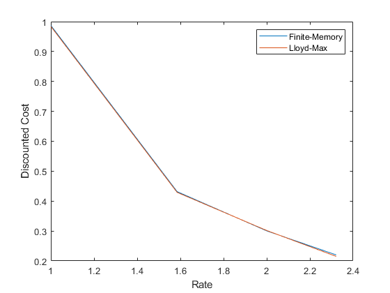
Figure 1: Finite-memory policy in i.i.d. case

Example 2 (Noisy Channel, Markov Source)

Here we will see that, even if $\delta(T)\leq\frac{1}{2}$, under an appropriate channel we may still have Dobrushin-type stability. Let $\mathbb{X}=\{0,\ldots,3\}$ and consider the source $(x_{t})_{t\geq 0}$ with transition kernel

$$T=\begin{pmatrix}\frac{1}{2}&\frac{1}{2}&0&0\\ \frac{1}{3}&\frac{1}{3}&\frac{1}{3}&0\\ \frac{1}{3}&\frac{1}{3}&0&\frac{1}{3}\\ \frac{1}{4}&\frac{1}{4}&\frac{1}{4}&\frac{1}{4}\end{pmatrix}.$$

We saw this matrix in the Dobrushin coefficient example, so we have $\delta(T)=\frac{1}{2}$, and we cannot use Corollary 2 immediately. However, consider $\mathcal{M}=\mathcal{M^{\prime}}=\{0,1\}$ with transition matrix $O(q^{\prime}|q)$ given by a binary symmetric channel with error probability $0.3$, i.e.,

$$O=\begin{pmatrix}\frac{7}{10}&\frac{3}{10}\\ \frac{3}{10}&\frac{7}{10}\end{pmatrix}.$$

This gives $\delta(O)=\frac{3}{5}$, so that $\alpha=(1-\frac{1}{2})(2-\frac{3}{5})=\frac{7}{10}<1$. Thus, we can use Corollary 2. Then through Theorem 2 and Corollary 2, our policy approaches the optimum as $N\to\infty$.

An optimal policy in this setup is not known, but we compare our algorithm to the scheme in [22], which uses Lloyd-Max type iterations along with an index assignment algorithm to obtain a so-called channel-optimized scalar quantizer (COSQ). We use the invariant distribution of the source to compute the COSQ. We can see that our policy performs better, and increases in performance as $N$ increases, as shown in Figure 2.

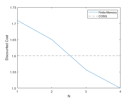
Figure 2: Finite-memory policy in Markov case

Example 3 (Memoryless Encoding)

Consider the same setup as the previous example but with

$$T=\begin{pmatrix}\frac{1}{2}&\frac{1}{6}&\frac{1}{6}&\frac{1}{6}\\ \frac{1}{3}&\frac{1}{3}&\frac{1}{3}&0\\ \frac{1}{3}&\frac{1}{3}&0&\frac{1}{3}\\ \frac{1}{4}&\frac{1}{4}&\frac{1}{4}&\frac{1}{4}\end{pmatrix}$$

and with $\mathcal{M}=\mathcal{M^{\prime}}=\mathbb{X}$, with channel $O(q^{\prime}|q)$ given by

$$O=\begin{pmatrix}\frac{7}{10}&\frac{1}{10}&\frac{1}{10}&\frac{1}{10}\\ \frac{1}{10}&\frac{7}{10}&\frac{1}{10}&\frac{1}{10}\\ \frac{1}{10}&\frac{1}{10}&\frac{7}{10}&\frac{1}{10}\\ \frac{1}{10}&\frac{1}{10}&\frac{1}{10}&\frac{7}{10}\end{pmatrix}$$

We have that $\delta(T)=\frac{2}{3}$ and $\delta(O)=\frac{4}{10}$, so we can apply Corollary 2 with $\alpha=(1-\frac{2}{3})(2-\frac{4}{10})=\frac{8}{15}$. In such a setup (where $\mathbb{X}=\mathcal{M}$ and the channel is symmetric), it was shown in [1] that “memoryless” encoding (i.e. where $q_{t}=x_{t}$) is optimal. We compare our algorithm against such an encoding policy, shown in Figure 3, and note that ours approches the optimum as $N$ increases.

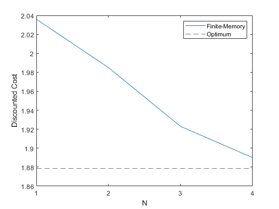
Figure 3: Finite-memory policy in “memoryless” case

Concluding Remarks

We have shown that our finite-memory policies outperform a COSQ, but the COSQ does not use channel feedback in its design. There exist other schemes, for example the adaptive COSQ (ACOSQ) in [23], which use feedback to obtain a lower distortion. However, this scheme is not strictly zero-delay as it uses the channel multiple times to send one source symbol. In the future, we would like to compare our finite-memory policies against more competitive zero-delay coding schemes that utilize feedback.

As mentioned in Section VI, the Dobrushin-type conditions are not a natural source of predictor stability in the zero-delay coding problem since they prioritize uninformative kernels. We would like to use observability-type conditions, such as those found in [14, 15], which prioritize informative kernels. While this method has been studied extensively in the control-free setup, the controlled setup is far more challenging due to policy dependence. In particular, we would like to generalize the notion of observability found in [14] to our setup, which would allow us to prove near-optimality of finite-memory policies for a larger class of zero-delay coding problems.

-A Proof of Lemma 1

Proof:

It can be shown that given the channel outputs $q^{\prime}_{[0,t]}$, the optimal decoder chooses $\hat{x}$ minimizing $\mathbf{E}^{\gamma}_{\pi_{0}}\left[d(x,\hat{x})|q^{\prime}_{[0,t]}\right]$. But this is exactly the expectation with respect to $\overline{\pi}_{t}$, so the optimal expected distortion at the decoder is

$$\min_{\hat{x}}\mathbf{E}^{\gamma}_{\pi_{0}}\left[d(x,\hat{x})|q^{\prime}_{[0,t]}\right]$$

$$=\; \min_{\hat{x}}\int_{\mathbb{X}}d(x,\hat{x})\overline{\pi}_{t}(dx)$$

$$=\; \min_{\hat{x}}\int_{\mathbb{X}}d(x,\hat{x})\frac{g_{Q_{t}}(x,q^{\prime}_{t})\varphi(z^{N}_{t})(dx)}{N(q^{\prime}_{t},Q_{t})},$$ (13)

where the second equality follows from our definition of $\varphi$ and the update equations (2). But at the encoder, we do not yet have $q^{\prime}_{t}$, so we need to take the expectation over $q^{\prime}_{t}$ conditioned on $(q^{\prime}_{[0,t-1]},Q_{t})$. Also, for any measurable $f:\mathcal{M^{\prime}}\to\mathbb{R}$,

$$\int_{\mathcal{M^{\prime}}}f(q^{\prime}_{t})P^{\gamma}_{\pi_{0}}(dq^{\prime}_{t}|q^{\prime}_{[0,t-1]},Q_{t})$$

$$=\; \int_{\mathcal{M^{\prime}}}\int_{\mathbb{X}}f(q^{\prime}_{t})P^{\gamma}_{\pi_{0}}(dq^{\prime}_{t},dx_{t}|q^{\prime}_{[0,t-1]},Q_{t})$$

$$=\; \iint_{\mathrlap{\mathcal{M^{\prime}}\times\mathbb{X}}}\;f(q^{\prime}_{t})P^{\gamma}_{\pi_{0}}(dq^{\prime}_{t}|x_{t},q^{\prime}_{[0,t-1]},Q_{t})P^{\gamma}_{\pi_{0}}(dx_{t}|q^{\prime}_{[0,t-1]},Q_{t})$$

$$=\; \int_{\mathcal{M^{\prime}}}\int_{\mathbb{X}}f(q^{\prime}_{t})O_{Q_{t}}(dq^{\prime}_{t}|x_{t})\pi_{t}(dx_{t})$$

$$=\; \int_{\mathcal{M^{\prime}}}f(q^{\prime}_{t})N(q^{\prime}_{t},Q_{t})\psi(dq^{\prime}_{t}),$$

where the third equality follows from the fact that $q^{\prime}_{t}$ depends on $q^{\prime}_{[0,t-1]}$ only through $x_{t}$ and $Q_{t}$, and that under a finite-memory policy $\gamma$, $x_{t}$ depends on $Q_{t}$ only through $q^{\prime}_{[0,t-1]}$. The final equality follows by using our definition of $g_{Q_{t}}(x_{t},q_{t})$ and $N(q^{\prime}_{t},Q_{t})$. Substituting (13) as $f(q^{\prime}_{t})$ in the above yields the result. ∎

-B Proof of Lemma 2

Proof:

Let $f:\mathcal{M}^{\prime}\to\mathbb{R}$ be measurable with $||f||_{\infty}\leq 1$. Then,

$$\left|\int_{\mathcal{M}^{\prime}}f(q^{\prime}_{t})P(dq^{\prime}_{t}|z^{N}_{t},Q_{t})-\int_{\mathcal{M}^{\prime}}f(q^{\prime}_{t})P(dq^{\prime}_{t}|\hat{z}^{N}_{t},Q_{t})\right|$$

$$= \begin{multlined}\Biggl{|}\int_{\mathbb{X}}\int_{\mathcal{M}^{\prime}}f(q^{\prime}_{t})P(dq^{\prime}_{t}|z^{N}_{t},x_{t},Q_{t})P(dx_{t}|z^{N}_{t},Q_{t})\\ -\int_{\mathbb{X}}\int_{\mathcal{M}^{\prime}}f(q^{\prime}_{t})P(dq^{\prime}_{t}|\hat{z}^{N}_{t},x_{t},Q_{t})P(dx_{t}|\hat{z}^{N}_{t},Q_{t})\Biggr{|}\end{multlined}\Biggl{|}\int_{\mathbb{X}}\int_{\mathcal{M}^{\prime}}f(q^{\prime}_{t})P(dq^{\prime}_{t}|z^{N}_{t},x_{t},Q_{t})P(dx_{t}|z^{N}_{t},Q_{t})\\ -\int_{\mathbb{X}}\int_{\mathcal{M}^{\prime}}f(q^{\prime}_{t})P(dq^{\prime}_{t}|\hat{z}^{N}_{t},x_{t},Q_{t})P(dx_{t}|\hat{z}^{N}_{t},Q_{t})\Biggr{|}$$

$$= \begin{multlined}\Biggl{|}\int_{\mathbb{X}}\int_{\mathcal{M}^{\prime}}f(q^{\prime}_{t})O_{Q_{t}}(dq^{\prime}_{t}|x_{t})\varphi(z^{N}_{t})(dx_{t})\\ -\int_{\mathbb{X}}\int_{\mathcal{M}^{\prime}}f(q^{\prime}_{N})O_{Q_{t}}(dq^{\prime}_{t}|x_{t})\varphi(\hat{z}^{N}_{t})(dx_{t})\Biggr{|}\end{multlined}\Biggl{|}\int_{\mathbb{X}}\int_{\mathcal{M}^{\prime}}f(q^{\prime}_{t})O_{Q_{t}}(dq^{\prime}_{t}|x_{t})\varphi(z^{N}_{t})(dx_{t})\\ -\int_{\mathbb{X}}\int_{\mathcal{M}^{\prime}}f(q^{\prime}_{N})O_{Q_{t}}(dq^{\prime}_{t}|x_{t})\varphi(\hat{z}^{N}_{t})(dx_{t})\Biggr{|}$$

$$\leq\; ||\varphi(z^{N}_{t})-\varphi(\hat{z}^{N}_{t})||_{TV},$$

where the third line follows from conditional independence of $q^{\prime}_{t}$ and $z^{N}_{t}$ given $(x_{t},Q_{t})$, and since $Q_{t}$ is a function of $z^{N}_{t}$ under a finite-memory policy. The last line follows from the fact that $g(x)\coloneqq\int_{\mathcal{M}^{\prime}}f(q^{\prime})O_{Q}(dq^{\prime}|x)$ is upper bounded by 1. Taking the supremum over all such $f$ yields the result. ∎

-C Proof of Theorem 1

Proof:

For simplicity, assume that $N=1$. To make the notation cleaner, we will omit this in the superscript. Then by (4), (5), and (6),

$$\widetilde{J}^{*}_{\beta}(z_{1})=\hat{J}^{*}_{\beta}(\hat{z}_{1})$$

$$=\min_{Q_{1}\in\mathcal{Q}}\left(c(\hat{z}_{1},Q_{1})+\beta\sum_{\mathclap{q^{\prime}_{1}\in\mathcal{M^{\prime}}}}\hat{J}^{*}_{\beta}(\hat{\pi},q^{\prime}_{1},Q_{1})P(q^{\prime}_{1}|\hat{z}_{1},Q_{1})\right)$$

Similarly,

$$J^{*}_{\beta}(z_{1})=J^{*}_{\beta}(z_{1})$$

$$= \min_{\mathclap{Q_{1}\in\mathcal{Q}}}\left(c(z_{1},Q_{1})+\beta\sum_{\mathclap{q^{\prime}_{1}\in\mathcal{M^{\prime}}}}J^{*}_{\beta}(\varphi(z_{1}),q^{\prime}_{1},Q_{1})P(q^{\prime}_{1}|z_{1},Q_{1})\right)$$

Also, using (6), we have $\hat{J}^{*}_{\beta}(\hat{\pi},q^{\prime}_{1},Q_{1})=\widetilde{J}_{\beta}^{*}(\varphi(z_{1}),q^{\prime}_{1},Q_{1})$, so we add and subtract

$$\sum_{q^{\prime}_{1}\in\mathcal{M^{\prime}}}\hat{J}^{*}_{\beta}(\hat{\pi},q^{\prime}_{1},Q_{1})P(q^{\prime}_{1}|z_{1},Q_{1})$$

$$= \sum_{q^{\prime}_{1}\in\mathcal{M^{\prime}}}\widetilde{J}^{*}_{\beta}(\varphi(z_{1}),q^{\prime}_{1},Q_{1})P(q^{\prime}_{1}|z_{1},Q_{1}),$$

to obtain

$$\left|\widetilde{J}^{*}_{\beta}(z_{1})-J^{*}_{\beta}(z_{1})\right|$$

$$\leq \max_{Q_{1}\in\mathcal{Q}}\left|c(\hat{z}_{1},Q_{1})-c(z_{1},Q_{1})\right|$$

$$\begin{multlined}+\max_{Q_{1}\in\mathcal{Q}}\beta\Biggl{|}\sum_{q^{\prime}_{1}\in\mathcal{M^{\prime}}}\hat{J}^{*}_{\beta}(\hat{\pi},q^{\prime}_{1},Q_{1})P(q^{\prime}_{1}|\hat{z}_{1},Q_{1})\\ -\sum_{q^{\prime}_{1}\in\mathcal{M^{\prime}}}\hat{J}^{*}_{\beta}(\hat{\pi},q^{\prime}_{1},Q_{1})P(q^{\prime}_{1}|z_{1},Q_{1})\Biggr{|}\end{multlined}+\max_{Q_{1}\in\mathcal{Q}}\beta\Biggl{|}\sum_{q^{\prime}_{1}\in\mathcal{M^{\prime}}}\hat{J}^{*}_{\beta}(\hat{\pi},q^{\prime}_{1},Q_{1})P(q^{\prime}_{1}|\hat{z}_{1},Q_{1})\\ -\sum_{q^{\prime}_{1}\in\mathcal{M^{\prime}}}\hat{J}^{*}_{\beta}(\hat{\pi},q^{\prime}_{1},Q_{1})P(q^{\prime}_{1}|z_{1},Q_{1})\Biggr{|}$$

$$\begin{multlined}+\max_{Q_{1}\in\mathcal{Q}}\beta\sum_{q^{\prime}_{1}\in\mathcal{M^{\prime}}}\Bigl{|}\widetilde{J}^{*}_{\beta}(\varphi(z_{1}),q^{\prime}_{1},Q_{1})\\ -J^{*}_{\beta}(\varphi(z_{1}),q^{\prime}_{1},Q_{1})\Bigr{|}P(q^{\prime}_{1}|z_{1},Q_{1}).\end{multlined}+\max_{Q_{1}\in\mathcal{Q}}\beta\sum_{q^{\prime}_{1}\in\mathcal{M^{\prime}}}\Bigl{|}\widetilde{J}^{*}_{\beta}(\varphi(z_{1}),q^{\prime}_{1},Q_{1})\\ -J^{*}_{\beta}(\varphi(z_{1}),q^{\prime}_{1},Q_{1})\Bigr{|}P(q^{\prime}_{1}|z_{1},Q_{1}).$$

Then using (7), we get

$$\mathbf{E}^{\gamma}_{\pi_{0}}\left[\left|\widetilde{J}^{*}_{\beta}(z_{1})-J^{*}_{\beta}(z_{1})\right|\right]$$

$$\leq\; \begin{multlined}||d||_{\infty}\mathbf{E}^{\gamma}_{\pi_{0}}\left[||\varphi(z_{1})-\varphi(\hat{z}_{1})||_{TV}\right]\\ +\max_{Q_{1}\in\mathcal{Q}}\beta||\hat{J}^{*}_{\beta}||_{\infty}\mathbf{E}_{\pi_{0}}^{\gamma}\left[||P(q^{\prime}_{1}|z_{1},Q_{1})-P(q^{\prime}_{1}|\hat{z}_{1},Q_{1})||_{TV}\right]\\ +\max_{Q_{1}\in\mathcal{Q}}\beta\mathbf{E}^{\gamma}_{\pi_{0}}\Biggl{[}\sum_{q^{\prime}_{1}\in\mathcal{M^{\prime}}}\Bigl{|}\widetilde{J}^{*}_{\beta}(\varphi(z_{1}),q^{\prime}_{1},Q_{1})\\ -J^{*}_{\beta}(\varphi(z_{1}),q^{\prime}_{1},Q_{1})\Bigr{|}P(q^{\prime}_{1}|z_{1},Q_{1})\Biggr{]}\end{multlined}||d||_{\infty}\mathbf{E}^{\gamma}_{\pi_{0}}\left[||\varphi(z_{1})-\varphi(\hat{z}_{1})||_{TV}\right]\\ +\max_{Q_{1}\in\mathcal{Q}}\beta||\hat{J}^{*}_{\beta}||_{\infty}\mathbf{E}_{\pi_{0}}^{\gamma}\left[||P(q^{\prime}_{1}|z_{1},Q_{1})-P(q^{\prime}_{1}|\hat{z}_{1},Q_{1})||_{TV}\right]\\ +\max_{Q_{1}\in\mathcal{Q}}\beta\mathbf{E}^{\gamma}_{\pi_{0}}\Biggl{[}\sum_{q^{\prime}_{1}\in\mathcal{M^{\prime}}}\Bigl{|}\widetilde{J}^{*}_{\beta}(\varphi(z_{1}),q^{\prime}_{1},Q_{1})\\ -J^{*}_{\beta}(\varphi(z_{1}),q^{\prime}_{1},Q_{1})\Bigr{|}P(q^{\prime}_{1}|z_{1},Q_{1})\Biggr{]}$$

$$\leq \begin{multlined}\left(||d||_{\infty}+\beta||\hat{J}^{*}_{\beta}||_{\infty}\right)\mathbf{E}_{\pi_{0}}^{\gamma}\left[||\varphi(z_{1})-\varphi(\hat{z}_{1})||_{TV}\right]\\ +\sup_{\gamma^{\prime}}\beta\mathbf{E}_{\pi_{0}}^{\gamma^{\prime}}\left[\left|\widetilde{J}^{*}_{\beta}(\varphi(z_{1}),q^{\prime}_{1},Q_{1})-J^{*}_{\beta}(\varphi(z_{1}),q^{\prime}_{1},Q_{1})\right|\right]\end{multlined}\left(||d||_{\infty}+\beta||\hat{J}^{*}_{\beta}||_{\infty}\right)\mathbf{E}_{\pi_{0}}^{\gamma}\left[||\varphi(z_{1})-\varphi(\hat{z}_{1})||_{TV}\right]\\ +\sup_{\gamma^{\prime}}\beta\mathbf{E}_{\pi_{0}}^{\gamma^{\prime}}\left[\left|\widetilde{J}^{*}_{\beta}(\varphi(z_{1}),q^{\prime}_{1},Q_{1})-J^{*}_{\beta}(\varphi(z_{1}),q^{\prime}_{1},Q_{1})\right|\right]$$

$$\leq \left(||d||_{\infty}+\beta||\hat{J}^{*}_{\beta}||_{\infty}\right)L_{0}+\sup_{\gamma^{\prime}}\beta\mathbf{E}_{\pi_{0}}^{\gamma^{\prime}}\left[\left|\widetilde{J}^{*}_{\beta}(z_{2})-J^{*}_{\beta}(z_{2})\right|\right]$$

where the second inequality follows from Lemma 2, and where we have again dropped the superscript on $L^{N}_{t}$. We repeat this process for $\mathbf{E}_{\pi_{0}}^{\gamma}\left[\left|\widetilde{J}^{*}_{\beta}(z_{2})-J^{*}_{\beta}(z_{2})\right|\right]$ to obtain

$$\mathbf{E}^{\gamma}_{\pi_{0}}\left[\left|\widetilde{J}^{*}_{\beta}(z_{1})-J^{*}_{\beta}(z_{1})\right|\right]$$

$$\leq \begin{multlined}\bigl{(}||d||_{\infty}+\beta||J^{*}_{\beta}||_{\infty}\bigr{)}L_{0}+\beta\left(||d||_{\infty}+\beta||J^{*}_{\beta}||_{\infty}\right)L_{1}\\ +\sup_{\gamma^{\prime}}\beta^{2}\mathbf{E}_{\pi_{0}}^{\gamma^{\prime}}\left[\left|\widetilde{J}^{*}_{\beta}(z_{3})-J^{*}_{\beta}(z_{3})\right|\right]\end{multlined}\bigl{(}||d||_{\infty}+\beta||J^{*}_{\beta}||_{\infty}\bigr{)}L_{0}+\beta\left(||d||_{\infty}+\beta||J^{*}_{\beta}||_{\infty}\right)L_{1}\\ +\sup_{\gamma^{\prime}}\beta^{2}\mathbf{E}_{\pi_{0}}^{\gamma^{\prime}}\left[\left|\widetilde{J}^{*}_{\beta}(z_{3})-J^{*}_{\beta}(z_{3})\right|\right].$$

Recursively, we get

$$\mathbf{E}^{\gamma}_{\pi_{0}}\left[\left|\widetilde{J}_{\beta}^{*}(z_{1})-J^{*}_{\beta}(z_{1})\right|\right]\leq(||d||_{\infty}+\beta||J^{*}_{\beta}||_{\infty})\sum_{t=0}^{\infty}\beta^{t}L_{t}.$$

Finally, we have from its definition that $||J^{*}_{\beta}||_{\infty}\leq\frac{||d||_{\infty}}{1-\beta}$, so we get

$$\mathbf{E}^{\gamma}_{\pi_{0}}\left[\left|\widetilde{J}^{*}_{\beta}(z_{1})-J^{*}_{\beta}(z_{1})\right|\right]\leq\frac{||d||_{\infty}}{1-\beta}\sum_{t=0}^{\infty}\beta^{t}L_{t}.$$

One can follow the same procedure to obtain the result for any $N\geq 1$. ∎

-D Proof of Theorem 2

Proof:

For simplicity, let $N=1$. Again, to make notation cleaner, we will omit this in the superscript. Also, let $Q_{1}^{*}\coloneqq\widetilde{\gamma}^{*}(z_{1})$. Then, by (3),

$$J_{\beta}(z_{1},\widetilde{\gamma}^{*})$$

$$= c(z_{1},Q^{*}_{1})+\beta\sum_{q^{\prime}_{1}\in\mathcal{M^{\prime}}}J_{\beta}((\varphi(z_{1}),q^{\prime}_{1},Q^{*}_{1}),\widetilde{\gamma}^{*})P(q^{\prime}_{1}|z_{1},Q^{*}_{1})$$

and using (5) and (6),

$$\widetilde{J}^{*}_{\beta}(z_{1})$$

$$= c(\hat{z}_{1},Q^{*}_{1})+\beta\sum_{q^{\prime}_{1}\in\mathcal{M^{\prime}}}\widetilde{J}^{*}_{\beta}(\varphi(z_{1}),q^{\prime}_{1},Q_{1}^{*})P(q^{\prime}_{1}|\hat{z}_{1},Q_{1}^{*}).$$

Let $z_{2}\coloneqq(\varphi(z_{1}),q^{\prime}_{1},Q_{1}^{*})$. Then we add and subtract

$$\sum_{q^{\prime}_{1}\in\mathcal{M^{\prime}}}\widetilde{J}^{*}_{\beta}(z_{2})P(q^{\prime}_{1}|z_{1},Q^{*}_{1}),$$

to obtain

$$\left|J_{\beta}(z_{1},\widetilde{\gamma}^{*})-\widetilde{J}^{*}_{\beta}(z_{1})\right|$$

$$\leq \begin{multlined}\left|c(z_{1},Q^{*}_{1})-c(\hat{z}_{1},Q^{*}_{1})\right|\\ +\beta\sum_{q^{\prime}_{1}\in\mathcal{M^{\prime}}}\left|\widetilde{J}^{*}_{\beta}(z_{2})P(q^{\prime}_{1}|\hat{z}_{1},Q_{1}^{*})-\widetilde{J}^{*}_{\beta}(z_{2})P(q^{\prime}_{1}|z_{1},Q_{1}^{*})\right|\\ +\beta\sum_{q^{\prime}_{1}\in\mathcal{M^{\prime}}}\left|\widetilde{J}^{*}_{\beta}(z_{2})-J_{\beta}(z_{2},\widetilde{\gamma}^{*})\right|P(q^{\prime}_{1}|z_{1},Q^{*}_{1}).\end{multlined}\left|c(z_{1},Q^{*}_{1})-c(\hat{z}_{1},Q^{*}_{1})\right|\\ +\beta\sum_{q^{\prime}_{1}\in\mathcal{M^{\prime}}}\left|\widetilde{J}^{*}_{\beta}(z_{2})P(q^{\prime}_{1}|\hat{z}_{1},Q_{1}^{*})-\widetilde{J}^{*}_{\beta}(z_{2})P(q^{\prime}_{1}|z_{1},Q_{1}^{*})\right|\\ +\beta\sum_{q^{\prime}_{1}\in\mathcal{M^{\prime}}}\left|\widetilde{J}^{*}_{\beta}(z_{2})-J_{\beta}(z_{2},\widetilde{\gamma}^{*})\right|P(q^{\prime}_{1}|z_{1},Q^{*}_{1}).$$

Thus, using (7) and Lemma 2,

$$\mathbf{E}^{\gamma}_{\pi_{0}}\left[\left|J_{\beta}(z_{1},\widetilde{\gamma}^{*})-\widetilde{J}^{*}_{\beta}(z_{1})\right|\right]$$

$$\leq \begin{multlined}||d||_{\infty}\sup_{\gamma^{\prime}}\mathbf{E}_{\pi_{0}}^{\gamma^{\prime}}\left[||\varphi(z_{1})-\varphi(\hat{z}_{1})||_{TV}\right]\\ +\beta||\widetilde{J}^{*}_{\beta}||_{\infty}\sup_{\gamma^{\prime}}\mathbf{E}_{\pi_{0}}^{\gamma^{\prime}}\left[||P(q^{\prime}_{1}|\hat{z}_{1},Q_{1}^{*})-P(q^{\prime}_{1}|z_{1},Q_{1}^{*})||_{TV}\right]\\ +\beta\sup_{\gamma^{\prime}}\mathbf{E}_{\pi_{0}}^{\gamma^{\prime}}\left[\left|\widetilde{J}^{*}_{\beta}(z_{2})-J_{\beta}(z_{2},\widetilde{\gamma}^{*})\right|\right]\end{multlined}||d||_{\infty}\sup_{\gamma^{\prime}}\mathbf{E}_{\pi_{0}}^{\gamma^{\prime}}\left[||\varphi(z_{1})-\varphi(\hat{z}_{1})||_{TV}\right]\\ +\beta||\widetilde{J}^{*}_{\beta}||_{\infty}\sup_{\gamma^{\prime}}\mathbf{E}_{\pi_{0}}^{\gamma^{\prime}}\left[||P(q^{\prime}_{1}|\hat{z}_{1},Q_{1}^{*})-P(q^{\prime}_{1}|z_{1},Q_{1}^{*})||_{TV}\right]\\ +\beta\sup_{\gamma^{\prime}}\mathbf{E}_{\pi_{0}}^{\gamma^{\prime}}\left[\left|\widetilde{J}^{*}_{\beta}(z_{2})-J_{\beta}(z_{2},\widetilde{\gamma}^{*})\right|\right]$$

$$\leq \begin{multlined}(||d||_{\infty}+\beta||\widetilde{J}^{*}_{\beta}||_{\infty})L_{0}\\ +\beta\sup_{\gamma^{\prime}}\mathbf{E}_{\pi_{0}}^{\gamma^{\prime}}\left[\left|J_{\beta}(z_{2},\widetilde{\gamma}^{*})-\widetilde{J}^{*}_{\beta}(z_{2})\right|\right]\end{multlined}(||d||_{\infty}+\beta||\widetilde{J}^{*}_{\beta}||_{\infty})L_{0}\\ +\beta\sup_{\gamma^{\prime}}\mathbf{E}_{\pi_{0}}^{\gamma^{\prime}}\left[\left|J_{\beta}(z_{2},\widetilde{\gamma}^{*})-\widetilde{J}^{*}_{\beta}(z_{2})\right|\right].$$

Recursively, and using the fact that $||\widetilde{J}^{*}_{\beta}||_{\infty}\leq\frac{||d||_{\infty}}{1-\beta}$,

$$\mathbf{E}^{\gamma}_{\pi_{0}}\left[\left|J^{*}_{\beta}(z_{1},\widetilde{\gamma}^{*})-J^{*}_{\beta}(z_{1})\right|\right] \leq\frac{||d||_{\infty}}{1-\beta}\sum_{t=0}^{\infty}\beta^{t}L_{t}.$$ (14)

Finally, we have

$$\mathbf{E}^{\gamma}_{\pi_{0}}\left[\left|J^{*}_{\beta}(z_{1},\widetilde{\gamma}^{*})-J^{*}_{\beta}(z_{1})\right|\right]$$

$$\leq \mathbf{E}^{\gamma}_{\pi_{0}}\left[\left|J^{*}_{\beta}(z_{1},\widetilde{\gamma}^{*})-\widetilde{J}^{*}_{\beta}(z_{1})\right|\right]+\mathbf{E}^{\gamma}_{\pi_{0}}\left[\left|\widetilde{J}^{*}_{\beta}(z_{1})-J^{*}_{\beta}(z_{1})\right|\right]$$

$$\leq \frac{2||d||_{\infty}}{1-\beta}\sum_{t=0}^{\infty}\beta^{t}L_{t},$$

where the final inequality follows from (14) and Theorem 1. Following the same procedure, we obtain the result for any $N\geq 1$. ∎

-E Proof of Lemma 3

Proof:

Let $f:\mathbb{X}\to\mathbb{R}$ be measurable with $||f||_{\infty}\leq 1$. Recall the update equations for $\pi_{t},\overline{\pi_{t}}$ given in (2). Then we have

$$\left|\int_{\mathbb{X}}f(x)\overline{\pi}^{\mu}_{t}(dx)-\int_{\mathbb{X}}f(x)\overline{\pi}^{\nu}_{t}(dx)\right|$$

$$= \left|\int_{\mathbb{X}}f(x)\frac{g_{Q_{t}}(x,q^{\prime}_{t})\pi^{\mu}_{t}(dx)}{N^{\mu}(q^{\prime}_{t},Q_{t})}-\int_{\mathbb{X}}f(x)\frac{g_{Q_{t}}(x,q^{\prime}_{t})\pi^{\nu}_{t}(dx)}{N^{\nu}(q^{\prime}_{t},Q_{t})}\right|$$

$$\leq \left|\int_{\mathbb{X}}f(x)\frac{g_{Q_{t}}(x,q^{\prime}_{t})\pi^{\mu}_{t}(dx)}{N^{\mu}(q^{\prime}_{t},Q_{t})}-\int_{\mathbb{X}}f(x)\frac{g_{Q_{t}}(x,q^{\prime}_{t})\pi^{\nu}_{t}(dx)}{N^{\mu}(q^{\prime}_{t},Q_{t})}\right|$$

$$\>+\left|\int_{\mathbb{X}}f(x)\frac{g_{Q_{t}}(x,q^{\prime}_{t})\pi^{\nu}_{t}(dx)}{N^{\mu}(q^{\prime}_{t},Q_{t})}-\int_{\mathbb{X}}f(x)\frac{g_{Q_{t}}(x,q^{\prime}_{t})\pi^{\nu}_{t}(dx)}{N^{\nu}(q^{\prime}_{t},Q_{t})}\right|$$

$$= \begin{multlined}\frac{1}{N^{\mu}(q^{\prime}_{t},Q_{t})}\Biggl{|}\int_{\mathbb{X}}f(x)g_{Q_{t}}(x,q^{\prime}_{t})\pi^{\mu}_{t}(dx)\\ -\int_{\mathbb{X}}f(x)g_{Q_{t}}(x,q^{\prime}_{t})\pi^{\nu}_{t}(dx)\Biggr{|}\end{multlined}\frac{1}{N^{\mu}(q^{\prime}_{t},Q_{t})}\Biggl{|}\int_{\mathbb{X}}f(x)g_{Q_{t}}(x,q^{\prime}_{t})\pi^{\mu}_{t}(dx)\\ -\int_{\mathbb{X}}f(x)g_{Q_{t}}(x,q^{\prime}_{t})\pi^{\nu}_{t}(dx)\Biggr{|}$$

$$+\begin{multlined}\Biggl{|}\frac{1}{N^{\mu}(q^{\prime}_{t},Q_{t})}-\frac{1}{N^{\nu}(q^{\prime}_{t},Q_{t})}\Biggr{|}\\ \cdot\left|\int_{\mathbb{X}}f(x)g_{Q_{t}}(x,q^{\prime}_{t})\pi^{\nu}_{t}(dx)\right|\end{multlined}\Biggl{|}\frac{1}{N^{\mu}(q^{\prime}_{t},Q_{t})}-\frac{1}{N^{\nu}(q^{\prime}_{t},Q_{t})}\Biggr{|}\\ \cdot\left|\int_{\mathbb{X}}f(x)g_{Q_{t}}(x,q^{\prime}_{t})\pi^{\nu}_{t}(dx)\right|$$

$$\leq \frac{1}{N^{\mu}(q^{\prime}_{t},Q_{t})}\int_{\mathbb{X}}g_{Q_{t}}(x,q^{\prime}_{t})|\pi^{\mu}_{t}-\pi^{\nu}_{t}|(dx)$$

$$+\left|\frac{1}{N^{\mu}(q^{\prime}_{t},Q_{t})}-\frac{1}{N^{\nu}(q^{\prime}_{t},Q_{t})}\right|N^{\nu}(q^{\prime}_{t},Q_{t})$$

$$\leq \frac{1}{N^{\mu}(q^{\prime}_{t},Q_{t})}\Biggl{(}\int_{\mathbb{X}}g_{Q_{t}}(x,q^{\prime}_{t})|\pi^{\mu}_{t}-\pi^{\nu}_{t}|(dx)$$

$$+\left|N^{\mu}(q^{\prime}_{t},Q_{t})-N^{\nu}(q^{\prime}_{t},Q_{t})\right|\Biggr{)}.$$

Taking the supremum over all $f$ gives

$$||\overline{\pi}^{\mu}_{t}-\overline{\pi}^{\nu}_{t}||_{TV}$$

$$\leq\begin{multlined}\frac{1}{N^{\mu}(q^{\prime}_{t},Q_{t})}\Bigl{(}\int_{\mathbb{X}}g_{Q_{t}}(x,q^{\prime}_{t})|\pi^{\mu}_{t}-\pi^{\nu}_{t}|(dx)\\ +\left|N^{\mu}(q^{\prime}_{t},Q_{t})-N^{\nu}(q^{\prime}_{t},Q_{t})\Bigr{|}\right).\end{multlined}\frac{1}{N^{\mu}(q^{\prime}_{t},Q_{t})}\Bigl{(}\int_{\mathbb{X}}g_{Q_{t}}(x,q^{\prime}_{t})|\pi^{\mu}_{t}-\pi^{\nu}_{t}|(dx)\\ +\left|N^{\mu}(q^{\prime}_{t},Q_{t})-N^{\nu}(q^{\prime}_{t},Q_{t})\Bigr{|}\right).$$ (17)

Then,

$$\int_{\mathbb{X}}\int_{\mathcal{M}^{\prime}}||\overline{\pi}^{\mu}_{t}-\overline{\pi}^{\nu}_{t}||_{TV}O_{Q_{t}}(q^{\prime}_{t}|x_{t})\pi^{\mu}_{t}(dx)$$

$$= \int_{\mathbb{X}}\int_{\mathcal{M}^{\prime}}||\overline{\pi}^{\mu}_{t}-\overline{\pi}^{\nu}_{t}||_{TV}g_{Q_{t}}(x,q^{\prime})\psi(dq^{\prime}_{t})\pi^{\mu}_{t}(dx)$$

$$= \int_{\mathcal{M}^{\prime}}||\overline{\pi}^{\mu}_{t}-\overline{\pi}^{\nu}_{t}||_{TV}\left(\int_{\mathbb{X}}g_{Q_{t}}(x,q^{\prime})\pi^{\mu}_{t}(dx)\right)\psi(dq^{\prime}_{t})$$

$$= \int_{\mathcal{M}^{\prime}}||\overline{\pi}^{\mu}_{t}-\overline{\pi}^{\nu}_{t}||_{TV}N^{\mu}(q^{\prime}_{t},Q_{t})\psi(dq^{\prime}_{t})$$

$$\leq \begin{multlined}\int_{\mathcal{M}^{\prime}}\Bigl{(}\int_{\mathbb{X}}g_{Q_{t}}(x,q^{\prime}_{t})|\pi^{\mu}_{t}-\pi^{\nu}_{t}|(dx)\\ +\left|N^{\mu}(q^{\prime}_{t},Q_{t})-N^{\nu}(q^{\prime}_{t},Q_{t})\right|\Bigr{)}\psi(dq^{\prime}_{t})\end{multlined}\int_{\mathcal{M}^{\prime}}\Bigl{(}\int_{\mathbb{X}}g_{Q_{t}}(x,q^{\prime}_{t})|\pi^{\mu}_{t}-\pi^{\nu}_{t}|(dx)\\ +\left|N^{\mu}(q^{\prime}_{t},Q_{t})-N^{\nu}(q^{\prime}_{t},Q_{t})\right|\Bigr{)}\psi(dq^{\prime}_{t})$$

$$\leq \begin{multlined}\int_{\mathbb{X}}\left(\int_{\mathcal{M}^{\prime}}g_{Q_{t}}(x,q^{\prime}_{t})\psi(dq^{\prime}_{t})\right)|\pi^{\mu}_{t}-\pi^{\nu}_{t}|(dx)\\ +\int_{\mathcal{M}^{\prime}}\left|\int_{\mathbb{X}}g_{Q_{t}}(x,q^{\prime}_{t})(\pi^{\mu}_{t}-\pi^{\nu}_{t})(dx)\right|\psi(dq^{\prime}_{t})\end{multlined}\int_{\mathbb{X}}\left(\int_{\mathcal{M}^{\prime}}g_{Q_{t}}(x,q^{\prime}_{t})\psi(dq^{\prime}_{t})\right)|\pi^{\mu}_{t}-\pi^{\nu}_{t}|(dx)\\ +\int_{\mathcal{M}^{\prime}}\left|\int_{\mathbb{X}}g_{Q_{t}}(x,q^{\prime}_{t})(\pi^{\mu}_{t}-\pi^{\nu}_{t})(dx)\right|\psi(dq^{\prime}_{t})$$

$$= ||\pi^{\mu}_{t}-\pi^{\nu}_{t}||_{TV}+\int_{\mathcal{M}^{\prime}}\left|\int_{\mathbb{X}}g_{Q_{t}}(x,q^{\prime}_{t})(\pi^{\mu}_{t}-\pi^{\nu}_{t})(dx)\right|\psi(dq^{\prime}_{t}).$$

Letting $S^{+}=\left\{q^{\prime}|\int_{\mathbb{X}}g_{Q_{t}}(x,q^{\prime}_{t})(\pi^{\mu}_{t}-\pi^{\nu}_{t})(dx)>0\right\}$ and $S^{-}=\left\{q^{\prime}|\int_{\mathbb{X}}g_{Q_{t}}(x,q^{\prime}_{t})(\pi^{\mu}_{t}-\pi^{\nu}_{t})(dx)\leq 0\right\}$, we get that $\mathbf{1}_{S^{+}}(q^{\prime})-\mathbf{1}_{S^{+}-}(q^{\prime})$ is a measurable function of $q^{\prime}$ bounded by $1$, so that

$$\int_{\mathcal{M}^{\prime}}\left|\int_{\mathbb{X}}g_{Q_{t}}(x,q^{\prime}_{t})(\pi^{\mu}_{t}-\pi^{\nu}_{t})(dx)\right|\psi(dq^{\prime}_{t})$$

$$= \begin{multlined}\int_{\mathcal{M}^{\prime}}\left(\mathbf{1}_{S^{+}}(q^{\prime})-\mathbf{1}_{S^{-}}(q^{\prime})\right)\\ \cdot\left(\int_{\mathbb{X}}g_{Q_{t}}(x,q^{\prime}_{t})(\pi^{\mu}_{t}-\pi^{\nu}_{t})(dx)\right)\psi(dq^{\prime}_{t})\end{multlined}\int_{\mathcal{M}^{\prime}}\left(\mathbf{1}_{S^{+}}(q^{\prime})-\mathbf{1}_{S^{-}}(q^{\prime})\right)\\ \cdot\left(\int_{\mathbb{X}}g_{Q_{t}}(x,q^{\prime}_{t})(\pi^{\mu}_{t}-\pi^{\nu}_{t})(dx)\right)\psi(dq^{\prime}_{t})$$

$$= \sup_{||f||_{\infty}\leq 1}\left|\int_{\mathbb{X}}\int_{\mathcal{M}^{\prime}}f(q^{\prime})O_{Q_{t}}(dq^{\prime}|x)(\pi^{\mu}_{t}-\pi^{\nu}_{t})(dx)\right|$$

$$= ||O_{Q_{t}}(\pi^{\mu}_{t})-O_{Q_{t}}(\pi^{\nu}_{t})||_{TV}\leq(1-\delta(O_{Q_{t}}))||\pi^{\mu}_{t}-\pi^{\nu}_{t}||_{TV},$$

where we have used (11) for the final inequality. Adding the two terms gives

$$\int_{\mathbb{X}}\int_{\mathcal{M}^{\prime}}||\overline{\pi}^{\mu}_{t}-\overline{\pi}^{\nu}_{t}||_{TV}g_{Q_{t}}(x,q^{\prime})\psi(dq^{\prime}_{t})\pi^{\mu}_{t}(dx)$$

$$\leq (2-\delta(O_{Q_{t}}))||\pi^{\mu}_{t}-\pi^{\nu}_{t}||_{TV}$$

$$\leq (2-\tilde{\delta}(O))||\pi^{\mu}_{t}-\pi^{\nu}_{t}||_{TV}.$$

∎

References

- [1] J. C. Walrand and P. Varaiya, “Optimal causal coding-decoding problems,” IEEE Transactions on Information Theory, vol. 19, pp. 814–820, 1983.
- [2] D. Teneketzis, “On the structure of optimal real-time encoders and decoders in noisy communication,” IEEE Transactions on Information Theory, vol. 52, pp. 4017–4035, September 2006.
- [3] R. G. Wood, T. Linder, and S. Yüksel, “Optimal zero delay coding of Markov sources: Stationary and finite memory codes,” IEEE Transactions on Information Theory, vol. 63, pp. 5968–5980, 2017.
- [4] A. Mahajan and D. Teneketzis, “Optimal design of sequential real-time communication systems,” IEEE Transactions on Information Theory, vol. 55, pp. 5317–5338, November 2009.
- [5] M. Ghomi, T. Linder, and S. Yüksel, “Zero-delay lossy coding of linear vector Markov sources: Optimality of stationary codes and near optimality of finite memory codes,” IEEE Transactions on Information Theory, vol. 68, no. 5, pp. 3474–3488, 2021.
- [6] N. Saldi, S. Yüksel, and T. Linder, “On the asymptotic optimality of finite approximations to Markov decision processes with Borel spaces,” Mathematics of Operations Research, vol. 42, no. 4, pp. 945–978, 2017.
- [7] N. Saldi, S. Yüksel, and T. Linder, “Finite model approximations for partially observed Markov decision processes with discounted cost,” IEEE Transactions on Automatic Control, vol. 65, 2020.
- [8] A. Kara, N. Saldi, and S. Yüksel, “Q-learning for MDPs with general spaces: Convergence and near optimality via quantization under weak continuity,” Journal of Machine Learning Research, 2023 (arXiv:2111.06781), 2021.
- [9] L. Cregg, F. Alajaji, and S. Yüksel, “Reinforcement learning for zero-delay coding over a noisy channel with feedback,” in IEEE Conference on Decision and Control, to appear, 2023.
- [10] N. Saldi, T. Linder, and S. Yüksel, Finite Approximations in Discrete-Time Stochastic Control: Quantized Models and Asymptotic Optimality. Cham: Springer, 2018.
- [11] A. Kara and S. Yüksel, “Convergence of finite memory Q-learning for POMDPs and near optimality of learned policies under filter stability,” Mathematics of Operations Research (also arXiv:2103.12158), 2023.
- [12] P. Chigansky and R. Liptser, “Stability of nonlinear filters in non-mixing case,” Annals of Applied Probability, vol. 14, pp. 2038–2056, 2004.
- [13] C. McDonald and S. Yüksel, “Exponential filter stability via Dobrushin’s coefficient,” Electronic Communications in Probability, vol. 25, 2020.
- [14] ——, “Stochastic observability and filter stability under several criteria,” IEEE Transactions on Automatic Control (to appear), arXiv:1812.01772, 2022.
- [15] ——, “Robustness to incorrect priors and controlled filter stability in partially observed stochastic control,” SIAM Journal on Control and Optimization, vol. 60, no. 2, pp. 842–870, 2022.
- [16] H. Yu and D. P. Bertsekas, “On near optimality of the set of finite-state controllers for average cost POMDP,” Mathematics of Operations Research, vol. 33, no. 1, pp. 1–11, 2008.
- [17] A. Kara and S. Yüksel, “Near optimality of finite memory feedback policies in partially observed Markov decision processes,” Journal of Machine Learning Research, vol. 23, no. 11, pp. 1–46, 2022.
- [18] O. Cappé, E. Moulines, and T. Rydén, Inference in Hidden Markov Models. Germany: Springer, 2005.
- [19] O. Hernández-Lerma and J. Lasserre, Discrete-Time Markov Control Processes: Basic Optimality Criteria. Springer, 1996.
- [20] R. Dobrushin, “Central limit theorem for nonstationary Markov chains. i,” Theory of Probability & Its Applications, vol. 1, no. 1, pp. 65–80, 1956.
- [21] C. J. C. H. Watkins and P. Dayan, “Q-learning,” Machine Learning, vol. 8, pp. 279–292, 1992.
- [22] N. Farvardin and V. Vaishampayan, “Optimal quantizer design for noisy channels: An approach to combined source - channel coding,” IEEE Transactions on Information Theory, vol. 33, no. 6, pp. 827–838, 1987.
- [23] A. Amanullah and M. Salehi, “Joint source-channel coding in the presence of feedback,” in Proceedings of 27th Asilomar Conference on Signals, Systems and Computers, vol. 2, 1993, pp. 930–934.