Adaptive Preconditioned Gradient Descent with Energy

Abstract.

We propose an adaptive time step with energy for a large class of preconditioned gradient descent methods, mainly applied to constrained optimization problems. Our strategy relies on representing the usual descent direction by the product of an energy variable and a transformed gradient, with a preconditioning matrix, for example, to reflect the natural gradient induced by the underlying metric in parameter space or to endow a projection operator when linear equality constraints are present. We present theoretical results on both unconditional stability and convergence rates for three respective classes of objective functions. In addition, our numerical results shed light on the excellent performance of the proposed method on several benchmark optimization problems.

1. Introduction

We introduce an adaptive time-step preconditioned gradient descent method for algorithms in the form of

$$\theta_{k+1}=\theta_{k}-\eta_{k}A_{k}^{\dagger}\nabla L(\theta_{k}),$$ (1.1)

applied to the optimization problem

$$\min_{\theta\in\Theta}L(\theta),$$ (1.2)

where $L\in C^{1}(\mathbb{R}^{n})$ is bounded below, $\Theta$ is a (constraint) set of all possible parameters, $A_{k}$ is a general preconditioning matrix and $A_{k}^{\dagger}$ is its Moore–Penrose inverse. Here, $\{\eta_{k}\}$ are step sizes (or learning rates), which play a key role in the algorithm’s convergence due to the gap between the continuous gradient flow equation and the discrete iteration. Typical choices for $\{\eta_{k}\}$ are either empirical schedules or damping techniques [27, Sec. 10]. Here, we propose an algorithm called AEPG, short for adaptive energy-based preconditioned gradient descent, which reads as follows

$$v_{k}=A_{k}^{\dagger}\nabla l(\theta_{k}),$$ (1.3a)

$$r_{k+1}=\frac{r_{k}}{1+2\eta\|v_{k}\|^{2}},$$ (1.3b)

$$\theta_{k+1}=\theta_{k}-2\eta r_{k+1}v_{k},$$ (1.3c)

where $l(\theta)=\sqrt{L(\theta)+c}$, $c\in\mathbb{R}$ such that $\inf\limits_{\theta\in\Theta}\left(L(\theta)+c\right)>0$, and $\eta>0$ is the base step size.

One common strategy for solving (1.2) is to apply simple iterative algorithms such as the standard gradient descent (GD), i.e., taking $A_{k}=I$ in (1.1),

$$\theta_{k+1}=\theta_{k}-\eta_{k}\nabla L(\theta_{k}).$$ (1.4)

However, if $\Theta$ represents a constraint set where the simple GD cannot guarantee the iterates to stay in, the projected gradient descent method (PGD) is also used:

$$\theta_{k+1}=\mathcal{P}_{\Theta}(\theta_{k}-\eta_{k}\nabla L(\theta_{k})),$$ (1.5)

where $\mathcal{P}_{\Theta}$ is the projection on $\Theta$. Under relatively mild assumptions on $L$ and $\Theta$, one can prove that (projected) GD with a fixed small step-size $\eta_{k}=\eta>0$ improves the quality of the iterates over time, $L(\theta_{k+1})<L(\theta_{k})$, and converges to a stationary point in $\Theta$, see, e.g., [35]. A more sophisticated version of the algorithm determines $\eta_{k}$ by searching for the minimum of the objective function along the descent direction [31].

While (projected) GDs are widely used, they suffer from two potential issues:

1. limitation on the step size due to only conditional stability of (P)GD;

2. descent directions, $-\nabla L(\theta_{k})$, do not adapt to the geometry of the problem.

Both issues can significantly slow down the convergence, especially in large-scale machine learning applications [38, 9]. These issues persist for the stochastic approximation of GD, called SGD. Indeed, in the Deep Learning community, SGD is widely used to reduce the computational cost of gradient computation via mini-batches, achieving faster iterations in exchange for a lower convergence rate. Additionally, the variance introduces extra challenges. See [14, 41, 40, 17, 2] for various adaptive strategies to boost the performance of SGD.

To solve issue (i), the authors in [23, 22] introduced the adaptive gradient descent with energy (AEGD): starting from $\theta_{0}$ and $r_{0}=l(\theta_{0})$ with $l(\theta)=\sqrt{L(\theta)+c}$, inductively define

$$v_{k} =\nabla l(\theta_{k}),$$ (1.6a)

$$r_{k+1} =\frac{r_{k}}{1+2\eta\|v_{k}\|^{2}},$$ (1.6b)

$$\theta_{k+1} =\theta_{k}-2\eta r_{k+1}v_{k},$$ (1.6c)

where $c\in\mathbb{R}$ is chosen so that $\inf\limits_{\theta\in\Theta}\left(L(\theta)+c\right)>0$.

In sharp contrast with (P)GD, such energy-adaptive gradient methods feature the unconditional energy stability property, irrespective of the base step size $\eta>0$. The excellent performance of AEGD-type schemes has been demonstrated with various optimization tasks [23, 22]. AEGD can be extended to account for stochastic effects in estimating the gradient [23] or incorporate momentum for a further convergence acceleration [22]. Additionally, results in [23] show that $c$ has little impact on the performance of (1.6).

Algorithms like (1.1) aim at tackling issue (ii) above by providing a better, geometrically motivated descent direction through a suitable choice of the preconditioning matrix $A_{k}$. In fact, (1.1) includes many classical and well-known optimization methods such as Newton and Gauss–Newton methods [31]. One such algorithm relevant to our study and discussed later in the paper is the Hessian–Riemannian gradient descent (HRGD) [3], which corresponds to $A_{k}=\nabla^{2}h(\theta_{k})$ for a suitable convex function $h$. Another algorithm in the form of (1.1) is the so-called natural gradient descent (NGD) method, which corresponds to setting $A_{k}=G(\theta_{k})$ where $G(\theta)$ is a geometrically motivated positive semidefinite matrix [32]. Hence, to address both limitations simultaneously, we develop an extension of AEGD, as given in (1.3), suitable for algorithms in the form (1.1). The proposed method (1.3) is unconditionally energy stable irrespective of $\eta$.

With the adaptive feature of AEPG, convergence is expected for a large set of choices for both $\eta$ and $r_{0}$. This leads to the following question:
What is the convergence rate of this preconditioned gradient descent method with adaptive time step with energy?
We prove that if $A_{k}$ is symmetric and positive definite, this adaptive method with suitably small step size converges to a minimum of the objective function, and convergence rates are affected by the geometry of the objective function. We obtain convergence rates for both convex and non-convex objectives, including those satisfying the Polyak–Lojasiewics (PL) condition. Similar results are also established when an additional linear equality constraint is imposed. In the latter case, the preconditioning matrix needs to be modified with a projection operator.

The first instance of application of (1.3) is HRGD. Assume that $\Theta=\mathcal{M}\cap\{\theta:~{}B\theta=b\}$, where $\mathcal{M}\subset\mathbb{R}^{n}$ is a closed convex set with a nonempty interior, $B\in\mathbb{R}^{n\times m}$, $b\in\mathbb{R}^{m}$, $m<n$, and $\operatorname{rank}(B)=m$. Furthermore, assume that $h:\operatorname{int}(\mathcal{M})\to\mathbb{R}$ is a smooth convex function with a non-degenerate Hessian such that $\lim\limits_{\theta\to\partial\mathcal{M}}|\nabla h(\theta)|=\infty$. Then $\nabla h$ is a diffeomorphism between $\operatorname{int}(\mathcal{M})$ and $\mathbb{R}^{n}$, and $\operatorname{int}(\mathcal{M})$ endowed with the metric $\nabla^{2}h(\theta)$ becomes the “warped” version of $\mathbb{R}^{n}$ with $\partial\mathcal{M}$ corresponding to $\infty$. Consequently, preconditioning the gradient by $A(\theta)=\nabla^{2}h(\theta)$ and projecting it on $\operatorname{ker}(B)$ enforces the gradient flow to stay in the relative interior of $\Theta$; that is, $\operatorname{int}(\mathcal{M})\cap\left\{\theta~{}:~{}B\theta=b\right\}$ [3]. Hence, the HRGD is given by

$$\theta_{k+1}=\theta_{k}-\eta_{k}P(\theta_{k})\nabla^{2}h(\theta_{k})^{-1}\nabla L(\theta_{k}),$$ (1.7)

where $P(\theta):\mathbb{R}^{n}\to\mathbb{R}^{n}$ is the $\nabla^{2}h(\theta)$-orthogonal projection on $\operatorname{ker}(B)$ [3]. More explicitly,

$$P(\theta)=I-\nabla^{2}h(\theta)^{-1}B^{\top}(B\nabla^{2}h(\theta)^{-1}B^{\top})^{-1}B.$$

In this case, we can apply (1.3) by choosing $v_{k}=P(\theta_{k})\nabla^{2}h(\theta_{k})^{-1}\nabla l(\theta_{k})$ to adaptively change the step size.

Our second instance of application of AEPG is NGD defined by

$$\theta_{k+1}=\theta_{k}-\eta_{k}G(\theta_{k})^{\dagger}\nabla L(\theta_{k}).$$ (1.8)

There are various choices for the matrix $G(\theta)$ based on the structure of the optimization problem (1.2). We are interested in cases when

$$L(\theta)=f(\phi(\theta)),\quad\theta\in\Theta,$$

where $\phi:\Theta\to\mathcal{M}$ is a smooth forward model, and $f:\mathcal{M}\to\mathbb{R}$ is a smooth function, such as a fidelity measure. When $(\mathcal{M},g)$ is a, possibly infinite-dimensional, (formal) Riemannian manifold, we can pull back the Riemannian metric on $(\mathcal{M},g)$ through $\phi$. That is,

$$G^{\phi}_{ij}(\theta)=\left\langle\partial^{g}_{\theta_{i}}\phi(\theta),\partial^{g}_{\theta_{j}}\phi(\theta)\right\rangle_{g(\phi(\theta))},\quad\theta\in\Theta,$$ (1.9)

where $\{\partial^{g}_{\theta_{i}}\phi(\theta)\}$ are the tangent vectors on the tangent space $T\mathcal{M}_{\phi(\theta)}$. This choice of the metric corresponds to the steepest descent as measured in the “natural metric” of the model-manifold $(\mathcal{M},g)$. Hence, there is a built-in robustness with respect to the parameterization $\theta\mapsto\phi(\theta)$ [32].

One particular example of interest is the Wasserstein NGD (WNGD), which corresponds to $\left(\mathcal{M},g\right)=\left(\mathcal{P}_{2}(\mathbb{R}^{d}),W_{2}\right)$; that is, the space of Borel probability measures with finite second moments equipped with the quadratic Wasserstein distance. WNGD has recently gained interest in light of machine learning and PDE-based optimization applications [19, 5, 18, 39, 45, 32]. These previous works focus on the computation of descent directions. Here, we focus on time steps and apply (1.3) to WNGD, incorporating efficient computation of $\{v_{k}\}$ by methods developed in [32]. We refer to Section 5 for more details on WNGD.

Our AEPG algorithm can also be applied to other types of problems, as long as a preconditioning matrix can be well-identified; for example, to the Laplacian smoothing gradient descent (LSGD) method [33], where the authors use $A=I-\sigma\Delta$ to reduce the variance of the SGD method, where $I$ is the $n\times n$ identity matrix and $\Delta$ is the discrete one-dimensional Laplacian.

Our approach consists of a novel combination of the preconditioned gradient and the energy-adaptive strategy. Such an approach allows us to accelerate the standard GD in both aspects with provable convergence rates under rather mild conditions on both the objective function and the step size. Our present results for constrained optimization problems provide some understanding of the energy-driven update rule coupled with the preconditioned gradient selection, which creates a path towards additional algorithms with AEGD-type techniques.

1.1. Contributions of the work

To sum up, our main contributions are as follows.

1. We propose a novel AEPG algorithm for (1.1) and establish its convergence theory in three distinct cases: general differentiable objective functions, nonconvex objective functions satisfying the Polyak–Lojasiewics (PL) condition, and convex objective functions.

2. We apply our method to HRGD and NGD, two particular optimization algorithms in the form of (1.1), improving these methods with unconditional stability.

3. We show that HRGD can be interpreted as an NGD and thus provide a unifying framework for studying various constrained optimization algorithms.

4. We conduct several numerical experiments and demonstrate that AEPG exhibits faster convergence than the classical algorithms without using an adaptive step size, especially on ill-conditioned or nonconvex problems.

1.2. Related literature

It is natural to search for a better descent direction to accelerate the convergence of GD. This can be achieved by using the curvature information of the objective function as in Newton and quasi-Newton methods. For $\alpha$-smooth objective functions, these two methods attain a quadratic and superlinear local convergence rate, respectively [31]. The natural gradient method originally introduced in [4] falls into this category with the curvature information given by the Riemannian metric tensor. The Wasserstein natural gradient has attracted many interests in recent years [19, 20, 32]. We refer the readers to [27] for more discussion on the natural gradient. Adding momentum is another technique that is commonly used to improve the descent direction, e.g., the heavy-ball (HB) method [34] and the Nesterov’s accelerated gradient (NAG) [28, 29].

Another category of work aiming to speed up the convergence of GD (or SGD) is to use adaptive step sizes. One technique is to make use of the historical gradients to adapt the step size with renowned works such as AdaGrad [14] and RMSProp [41]. Adam [17] combines the benefits of both the momentum and adaptive step size, exhibiting fast convergence in the early stage of the iteration, and is widely used by the machine learning community. For further improvements of Adam, see [13, 36, 24, 25, 47]. These adaptive methods not only update the step size in each iteration, but also compute an individual step size for each parameter. Other adaptive techniques adjust the step size based on the error of the objective function value [4, 44].

Manifold optimization has also been extensively studied in the literature. The general feasible algorithm framework on the manifold lies in using a retraction operator (with the help of parallel translation or vector transport) to pull the update back to the manifold constraint. In practice, different retraction operators’ computational costs and convergence behavior vary greatly; we refer to [15, 1, 8, 16, 21] and references therein for further details.

Finally, we mention a considerable body of work concerning the related but distinct strategy of improving GD for unconstrained optimization problems. For line search-based GD methods, we recall the classical Armijo rule (1966) and the Wolfe conditions (1969) to guide the inexact line search, also referring to [46, 30], the book of [31], and the references therein. Another notable gradient method with modified step sizes is the so-called BB method [6], which is motivated by Newton’s method but does not involve any Hessian. There are also numerous studies of various methods that can handle constraints (inequality or equality constraints or a mixture of both), such as projected gradient descent, proximal gradient methods, penalty methods, barrier methods, sequential quadratic programming (SQP) methods, interior-point methods, augmented Lagrangian/multiplier methods, the primal-dual strategies, and the active set strategies; see, e.g., [7, 31]. Thus, our work also contributes to the field of continuous optimization with constraints.

1.3. Notations

Throughout this paper, we use $\|\cdot\|$ to denote the $\ell^{2}$ norm for vectors and the spectral norm for matrices, respectively. Moreover, we use $\lambda_{1}(\cdot),\ldots,\lambda_{n}(\cdot)$ to denote the smallest and largest eigenvalues, respectively. For a function $L$, we use $\nabla L$ and $\nabla^{2}L$ to denote its gradient and Hessian, and $L^{*}$ to denote a global minimum value of $L$. For a positive definite matrix $A$, we define the vector induced norm by the matrix $A$ as $\|w\|_{A}:=\sqrt{\langle w,Aw\rangle}$. List $\{1,2,\cdots,n\}$ is denoted by $[n]$.

1.4. Organization.

The rest of the paper is organized as follows. Section 2 presents the AEPG method and the main theoretical results, including unconditional energy stability, convergence, and convergence rates. In Section 3, we focus on HRGD, demonstrating that a certain type of constrained optimization problem can be solved by AEPG using a Hessian–Riemannian metric. Section 4 focuses on optimization with the nonlinear equality constraint and the use of NGD for such problems. In particular, Section 5 discusses the Wasserstein natural gradient and an efficient numerical method for computation through AEPG. Numerical results and examples are given in Section 6. Conclusions and further discussions follow in Section 7. Most technical proofs of theoretical results in Section 2 are deferred to Appendix A. A showcase of computing two-dimensional natural gradients is given in Appendix B. In Appendix C, we discuss natural gradient for general Riemannian manifold. Finally, in Appendix D, we include an example to illustrate the projected PL condition.

2. Preconditioned AEGD and theoretical results

In this section, we present the main preconditioned AEGD algorithm and the theoretical results on stability, convergence, and convergence rates. Throughout the paper, we assume that the objective function $L$ is differentiable and bounded from below.

We consider general preconditioned matrices $(A_{k})_{k=0}^{\infty}$ and assume that they are symmetric and uniformly positive definite, namely, there exists $\lambda_{1},\lambda_{n}>0$ such that

$$\lambda_{1}\|\xi\|^{2}\leq\xi^{\top}A_{k}\xi\leq\lambda_{n}\|\xi\|^{2},\quad\forall\xi\in\mathbb{R}^{n},~{}k\geq 0.$$ (2.1)

Hence $(A_{k})_{k=0}^{\infty}$ are invertible, and the associated preconditioned GD reads as

$$\theta_{k+1}=\theta_{k}-\eta A_{k}^{-1}\nabla L(\theta_{k}).$$ (2.2)

2.1. Formulation

As in AEGD (1.6) we set $l(\theta)=\sqrt{L(\theta)+c}$, where $c\in\mathbb{R}$ is chosen such that $\inf\limits_{\Theta}L+c>0$. Taking $v_{k}$ in the preconditioned gradient direction, we have the update rule following (1.3) where $A_{k}^{\dagger}$ becomes $A_{k}^{-1}$.

For the Hessian-Riemannian metric we choose $A_{k}=\nabla^{2}h(\theta_{k})$ (see Section 3), and for the Wasserstein metric we choose $A_{k}=G(\theta_{k})$ (see Section 5). We will also discuss how to modify the preconditioning matrix $A_{k}^{-1}$ when an equality constraint is explicitly given.

We start by discussing key properties of the algorithm (1.3).

2.2. No equality constraints

In this section, we assume that $\Theta$ is a closure of an open set in $\mathbb{R}^{n}$. The problem with equality constraints is discussed in Section 2.3.

Theorem 2.1 (Unconditional energy stability).

AEPG (1.3) is unconditionally energy stable in the sense that for any step size $\eta>0$,

$$r^{2}_{k+1}=r^{2}_{k}-(r_{k+1}-r_{k})^{2}-\frac{1}{\eta}\|\theta_{k+1}-\theta_{k}\|^{2}.$$ (2.3)

That is, $r_{k}$ is strictly decreasing and convergent with $r_{k}\to r^{*}$ as $k\to\infty$. Moreover,

$$\sum_{k=0}^{\infty}\|\theta_{k+1}-\theta_{k}\|^{2}\leq\eta r^{2}_{0}.\quad\Longrightarrow\quad\lim_{k\to\infty}\|\theta_{k+1}-\theta_{k}\|=0.$$ (2.4)

Proof.

From (1.3), it follows

$$2r_{k+1}(r_{k+1}-r_{k})=2r_{k+1}v_{k}^{\top}(\theta_{k+1}-\theta_{k})=-\frac{1}{\eta}\|\theta_{k+1}-\theta_{k}\|^{2}.$$

Upon rewriting with $2b(b-a)=b^{2}-a^{2}+(b-a)^{2}$, we obtain equality (2.3). From this, we see that $r^{2}_{k}$ is monotonically decreasing (also bounded below), therefore convergent; so does $r_{k}$ since $r_{k}\geq 0$. Summation of (2.3) over $k$ from $0,1,\cdots$ yields (2.4). ∎

Note that from (1.3b) one obtains

$$r_{0}-r^{*}=2\eta\sum_{j=0}^{\infty}r_{j+1}\|v_{j}\|^{2}\Rightarrow\lim_{k\to\infty}(r_{k+1}\|v_{k}\|^{2})=0.$$

In other words, after finite number of steps, either $\|v_{k}\|^{2}$ becomes small or $r_{k}$ becomes small. To ensure convergence to a stationary point for general objectives ($\|v_{k}\|^{2}\to 0$), we would have to make sure $r_{k}$ does not decrease too fast. This can be achieved with a modest upper bound for the base step size $\eta$.

In Lemma 2.2, we identify a sufficient condition on $\eta$ that ensures a positive lower bound for $(r_{k})_{k=0}^{\infty}$, which is essentially used in the convergence proof of Theorem 2.4. It is here we need the $\alpha$-smoothness assumption. We say $L$ is $\alpha$-smooth if $\|\nabla^{2}L(\theta)\|\leq\alpha$ for any $\theta\in\mathbb{R}^{n}$. Below we denote $L^{*}:=\inf\limits_{\Theta}L$ and assume $c$ is chosen such that $l^{*}:=\sqrt{L^{*}+c}>0$.

Lemma 2.2.

Suppose $L$ is $\alpha$-smooth, bounded from below by $L^{*}$, and $r_{k}$ generated by AEPG (1.3) with $r_{0}\geq\frac{L(\theta_{0})-L^{*}}{2l^{*}\lambda_{1}}$ satisfies

$$r_{k}\geq r^{*}>0,$$ (2.5)

provided

$$\eta<\eta_{s}:=\frac{2(2r_{0}l^{*}\lambda_{1}-L(\theta_{0})+L^{*})}{\alpha r_{0}^{2}},$$ (2.6)

where $\lambda_{1}>0$ is the smallest eigenvalue of $A(\theta)$ for all $\theta=\theta_{k}$.

Proof.

Using the $\alpha$-smoothness of $L$, we have

$$L(\theta_{j+1})\leq L(\theta_{j})+\nabla L(\theta_{j})^{\top}(\theta_{j+1}-\theta_{j})+\frac{\alpha}{2}\|\theta_{j+1}-\theta_{j}\|^{2}.$$ (2.7)

From (1.3a), we have $\nabla L(\theta_{j})=2l(\theta_{j})\nabla l(\theta_{j})=2l(\theta_{j})A_{j}v_{j}$. Hence,

$$\nabla L(\theta_{j})^{\top}(\theta_{j+1}-\theta_{j}) =2l(\theta_{j})(A_{j}v_{j})^{\top}(-2\eta r_{j+1}v_{j})$$

$$=-4\eta l(\theta_{j})r_{j+1}\,v_{j}^{\top}A_{j}v_{j}$$

$$\leq-4\eta l^{*}\lambda_{1}r_{j+1}\|v_{j}\|^{2}$$ (2.8)

$$=2l^{*}\lambda_{1}(r_{j+1}-r_{j}),$$

where the last equality follows from a formulation of (1.3b). Substitute (2.2) into (2.7) and take a summation over $j$ from $0$ to $k-1$,

$$L(\theta_{k})-L(\theta_{0}) \leq 2l^{*}\lambda_{1}(r_{k}-r_{0})+\frac{\alpha}{2}\sum_{j=0}^{k-1}\|\theta_{j+1}-\theta_{j}\|^{2}$$

$$\leq 2l^{*}\lambda_{1}(r_{k}-r_{0})+\frac{\alpha\eta}{2}r^{2}_{0},$$

where the last inequality is by (2.4). Using $L(\theta_{k})\geq L^{*}$, we have

$$r_{k} \geq r_{0}-\frac{L(\theta_{0})-L^{*}}{2l^{*}\lambda_{1}}-\frac{\alpha\eta}{4l^{*}\lambda_{1}}r^{2}_{0}=\frac{\alpha r_{0}^{2}}{4l^{*}\lambda_{1}}(\eta_{s}-\eta)>0.$$

Since this is a uniform lower bound for $r_{k}$, we let $k\to\infty$ to obtain (2.5). ∎

Remark 2.3.

If one takes the default choice $l(\theta_{0})$ for $r_{0}$ (consistent with the method derivation), the resulting lower bound for $r_{0}$ is equivalent to the following

$$\sqrt{L^{*}+c}\sqrt{L(\theta_{0})+c}>\frac{L(\theta_{0})-L^{*}}{2\lambda_{1}}.$$

That is

$$c>\frac{L(\theta_{0})-L^{*}}{2}\left(\sqrt{1+\lambda_{1}^{-2}}-1\right)-L^{*},$$

which clearly holds true by taking $c$ suitably larger than $-L^{*}$.

Theorem 2.4.

Under the same assumptions as in Lemma 2.2 with $r_{0}\geq\frac{L(\theta_{0})-L^{*}}{2l^{*}\lambda_{1}}$, let $(\theta_{k})_{k=0}^{\infty}$ be generated by AEPG (1.3). Then $(L(\theta_{k}))_{k=0}^{\infty}$ monotonically converges to a local minimum value of $L$ if

$$0<\eta\leq\min\bigg{\{}\eta_{0},\eta_{s}\bigg{\}},\quad\eta_{0}:=\frac{\lambda_{1}l^{*}}{\alpha r_{0}}.$$ (2.9)

Proof.

If $\eta\leq\eta_{0}$, the effective learning rate can be shown to fall into the regime that $L(\theta_{k})$ is decreasing, hence convergent. With $r_{0}\geq\frac{L(\theta_{0})-L^{*}}{2l^{*}\lambda_{1}}$ and $\eta\leq\eta_{s}$, Lemma 2.2 ensures that $r_{k}$ is bounded below by a positive constant so that $\|\nabla L(\theta_{k})\|^{2}$ converges to zero as $k$ tends to infinity. For the readers’ convenience, we include details of the proof in Appendix A.1. ∎

We now discuss the convergence rate of AEPG with further geometrical information on $L$, such as convexity or the Polyak–Lojasiewics (PL) property. For a differentiable function $L:\mathbb{R}^{n}\to\mathbb{R}$ with $\arg\min L\neq\emptyset$, i.e., the optimization problem has at least one global minimizer, we say $L$ satisfies the PL condition if there exists $\mu>0$ such that

$$\frac{1}{2}\|\nabla L(\theta)\|^{2}\geq\mu(L(\theta)-L(\theta^{*})),\quad\forall\theta\in\mathbb{R}^{n},\quad\forall\theta^{*}\in\arg\min L.$$ (2.10)

This means that $\nabla L(\theta)=0$ implies $L(\theta)=L(\theta^{*})$ or $\theta\in\arg\min L$. In other words, critical points are global minimizers.

Note that strongly convex functions ($\nabla^{2}f\geq\mu I$) satisfy the PL condition (2.10), while a function that satisfies the PL condition might be nonconvex. For example,

$$L(\theta)=\theta^{2}+3\sin^{2}\theta,\quad\theta\in\mathbb{R},$$

is not convex but satisfies the PL condition with $\mu=\frac{1}{32},~{}\min L=0$.

Theorem 2.5.

Assume $(\theta_{k})_{k=0}^{\infty}\subset\Theta$ when $\Theta\neq\mathbb{R}^{n}$. The convergence rates of AEPG (1.3) are given in three distinct scenarios:
(i) For any $\eta>0$ and $r_{0}>0$, we have

$$\min_{j<k}\|\nabla L(\theta_{j})\|^{2}\leq\frac{2r_{0}\lambda^{2}_{n}}{\eta r_{k}k}\left(\max_{j<k}L(\theta_{j})+c\right),$$ (2.11)

with $\lambda_{n}$ given in (2.1). Under the assumptions of Theorem 2.4 with $\eta$ satisfying (2.9), we have $r_{k}>r^{*}>0$, and the following convergence rates:
(ii) If $L$ is PL with a global minimizer $\theta^{*}$, then $\{\theta_{k}\}$ satisfies (2.12), hence convergent:

$$\sum_{k=0}^{\infty}\|\theta_{k+1}-\theta_{k}\|\leq\frac{4\lambda_{n}}{\sqrt{2\mu}\lambda_{1}}\sqrt{L(\theta_{0})-L(\theta^{*})},$$ (2.12)

$$L(\theta_{k})-L(\theta^{*})\leq e^{-c_{0}kr_{k}/\lambda_{n}}(L(\theta_{0})-L(\theta^{*})),\quad c_{0}:=\frac{\mu\eta}{l(\theta_{0})}.$$

(iii) If $L$ is convex with a minimizer $\theta^{*}$, then

$$L(\theta_{k})-L(\theta^{*})\leq\frac{c_{1}\lambda_{n}\|\theta_{0}-\theta^{*}\|^{2}}{kr_{k}},\quad c_{1}=\frac{2l(\theta_{0})}{\eta}.$$ (2.13)

Proof.

The proof of (ii) and (iii) is more or less standard, and hence deferred to Appendix A.2. Here we present a proof of (i).

(i) Using scheme (1.3b) we have

$$r_{j+1}-r_{j}=-2\eta r_{j+1}\|v_{j}\|^{2}.$$

Take a summation over $j$ from $0$ to $k-1$ gives

$$r_{0}-r_{k}=2\eta\sum_{j=0}^{k-1}r_{j+1}\|v_{j}\|^{2}\geq 2\eta r_{k}\sum_{j=0}^{k-1}\|v_{j}\|^{2}\geq\frac{2\eta r_{k}}{\lambda^{2}_{n}}\sum_{j=0}^{k-1}\|\nabla l(\theta_{j})\|^{2},$$

which upon rearrangement leads to

$$k\min_{j<k}\|\nabla l(\theta_{j})\|^{2}\leq\sum_{j=0}^{k-1}\|\nabla l(\theta_{j})\|^{2}\leq\frac{r_{0}\lambda^{2}_{n}}{2\eta r_{k}}.$$

Using $4l^{2}\|\nabla l\|^{2}=\|\nabla L\|^{2}$, and dividing $k$ on both sides gives (2.11). ∎

Remark 2.6.

(a) In contrast to GD with a fixed step size, which is set above as a hard upper threshold governed by the (generally unknown) smoothness constant $\alpha$, the standard GD algorithm might not converge. With AEPG, the result in (i) shows no dependence on such $\alpha$.

(b) As for the upper bound in (2.11), we can actually establish the following:

$$L(\theta_{k})\leq L(\theta_{0})+\frac{\alpha\eta^{2}r_{0}^{2}}{2},$$ (2.14)

provided $L$ is $\alpha$-smooth. In fact, using the $\alpha$-smoothness of $L$ and the fact that the search is in the descent direction, we have

$$L(\theta_{j+1})\leq L(\theta_{j})+\nabla L(\theta_{j})^{\top}(\theta_{j+1}-\theta_{j})+\frac{\alpha}{2}\|\theta_{j+1}-\theta_{j}\|^{2}\leq L(\theta_{j})+\frac{\alpha}{2}\|\theta_{j+1}-\theta_{j}\|^{2}.$$

Taking a summation over $j$ from $0$ to $k-1$ and using (2.4),

$$L(\theta_{k})-L(\theta_{0}) \leq\frac{\alpha}{2}\sum_{j=0}^{k-1}\|\theta_{j+1}-\theta_{j}\|^{2}\leq\frac{\alpha\eta}{2}r^{2}_{0}.$$

We should point out that such bound is unavailable for GD unless the step size is small.

(c) We should emphasize that the above results also hold for a variable $\eta$ as long as it is bounded by the threshold (2.9) and not so small. The convergence theory with variable $\eta$ allows us to consider rescheduling $\eta$ whenever there is such a need. For instance, we need $(\theta_{k})_{k=0}^{\infty}\subset\Theta$ when $\Theta\neq\mathbb{R}^{n}$. Indeed, in Algorithm 1 which we will present in Section 3.2, $\eta$ is chosen according to the line search at every iteration.

2.3. Equality constraints

In this section, we discuss specific preconditioning matrices for constrained optimization problems. We omit the explicit dependence on independent variables whenever there is no ambiguity.

Assume that

$$\Theta=\mathcal{M}\cap\{\theta\in\mathbb{R}^{n}~{}|~{}q(\theta)=0\},$$ (2.15)

where $\mathcal{M}\subset\mathbb{R}^{n}$ is a closure of an open set, and $q:\mathcal{M}\to\mathbb{R}^{m}$ is a smooth mapping such that $m<n$. Hence (1.2) reduces to

$$\min_{\theta}\{L(\theta)\;|\;\theta\in\mathcal{M},~{}q(\theta)=0\}.$$ (2.16)

Furthermore, assume $\mathcal{M}$ is endowed with a Riemannian structure given by a metric tensor $G(\theta)$, $\theta\in\mathcal{M}$. More specifically, for $\theta\in\mathcal{M}$ we have an inner product

$$\langle v_{1},v_{2}\rangle_{G(\theta)}=v_{1}^{\top}G(\theta)v_{2},\quad v_{1},v_{2}\in T_{\theta}\mathcal{M},$$ (2.17)

where $T_{\theta}\mathcal{M}\cong\mathbb{R}^{n}$ is the tangent space of $\mathcal{M}$ at $\theta$. Note that

$$T_{\theta}\Theta\cong\operatorname{ker}(Dq(\theta))=\{v\in\mathbb{R}^{n}~{}|~{}Dq(\theta)v=0\},$$

where $Dq(\theta)\in\mathbb{R}^{m\times n}$ is the Jacobian of $q$ at $\theta\in\mathcal{M}$.

Our goal is to choose $A_{k}^{\dagger}$ in (1.3) so that $v_{k}=A_{k}^{\dagger}\nabla l(\theta_{k})\in T_{\theta_{k}}\Theta$. Hence, we choose

$$A_{k}^{\dagger}=P(\theta_{k})G(\theta_{k})^{-1},$$ (2.18)

where $P(\theta):T_{\theta}\mathcal{M}\to T_{\theta}\Theta$ is the $G(\theta)$-orthogonal projection operator. Recall that the projection operator admits an explicit form

$$P(\theta)=I-G(\theta)^{-1}Dq(\theta)^{\top}(Dq(\theta)G(\theta)^{-1}Dq(\theta)^{\top})^{-1}Dq(\theta).$$ (2.19)

Such choice for $A_{k}^{\dagger}$ is motivated by the following lemma.

Lemma 2.7.

For every smooth $f:\mathbb{R}^{n}\to\mathbb{R}$ one has that

$$\operatorname{arg}\min_{v}\left\{\frac{df(\theta)}{dt}~{}\bigg{|}~{}\dot{\theta}=v,~{}v\in T_{\theta}\Theta,~{}\|v\|_{G(\theta)}\leq 1\right\}=-\frac{P(\theta)G(\theta)^{-1}\nabla f(\theta)}{\|P(\theta)G(\theta)^{-1}\nabla f(\theta)\|_{G(\theta)}}.$$

Hence, the steepest descent direction of $f$ on the submanifold $(\Theta,G)$ is $-P(\theta)G(\theta)^{-1}\nabla f(\theta)$.

Proof.

We have that

$$\begin{split}\frac{df(\theta)}{dt}=v^{\top}\nabla f(\theta)=v^{\top}G(\theta)G(\theta)^{-1}\nabla f(\theta)=\langle v,G(\theta)^{-1}\nabla f(\theta)\rangle_{G(\theta)}=\langle v,\nabla^{G}f(\theta)\rangle_{G(\theta)},\end{split}$$

where we denote by $\nabla^{G}f(\theta)=G(\theta)^{-1}\nabla f(\theta)$, the metric gradient. So we have the problem

$$\begin{split}&\operatorname{arg}\min_{v}\left\{\langle v,\nabla^{G}f(\theta)\rangle_{G(\theta)}~{}\bigg{|}~{}v\in T_{\theta}\Theta,~{}\|v\|_{G(\theta)}\leq 1\right\}\\ =&\operatorname{arg}\min_{v}\left\{\langle v,P(\theta)\nabla^{G}f(\theta)\rangle_{G(\theta)}~{}\bigg{|}~{}v\in T_{\theta}\Theta,~{}\|v\|_{G(\theta)}\leq 1\right\}\\ =&-\frac{P(\theta)\nabla^{G}f(\theta)}{\|P(\theta)\nabla^{G}f(\theta)\|_{G(\theta)}}=-\frac{P(\theta)G(\theta)^{-1}\nabla f(\theta)}{\|P(\theta)G(\theta)^{-1}\nabla f(\theta)\|_{G(\theta)}},\end{split}$$

where the first equation follows from the definition of the orthogonal projection. ∎

Remark 2.8.

As mentioned above, the choice (2.18) in (1.3) yields $\theta_{k+1}-\theta_{k}=-2\eta r_{k+1}v_{k}\in T_{\theta_{k}}\Theta$. However, $\Theta$ might be curved due to a non-affine $q$, which means that $q(\theta_{k+1})\not=0$, and $\theta_{k+1}\notin\Theta$ in general. Therefore (1.3) returns feasible updates only when $q(\theta)=B\theta-b$.

The following theorem summarizes stability and convergence properties of (1.3) for the case (2.18).

Theorem 2.9.

Let $G$ be symmetric and positive definite with $0<\lambda_{1}\leq\|G(\theta)\|_{2}\leq\lambda_{n}$, and

$$\theta_{0}\in\Theta=\{\theta\in\mathcal{M},\;B\theta=b\}.$$

Furthermore, let $\theta_{k}$ be generated by (1.3) with (2.18). Then we have that

• It is unconditionally energy stable as stated in Theorem 2.1.

• The statement in Lemma 2.2 about a positive lower bound for $r_{k}$ still holds.

• Under the same assumptions and condition on $\eta$ as described in Theorem 2.4, $L(\theta_{k})$ decreases monotonically and converges towards a local minimum value of $L$ with

  $$\lim_{k\to\infty}\|P_{k}^{\top}\nabla L(\theta_{k})\|\to 0.$$

• We have convergence rates in three distinct scenarios:

  • For any $\eta>0$ and $r_{0}>0$, we always have

    $$\min_{j<k}\|P_{j}^{\top}\nabla L(\theta_{j})\|^{2}\leq\frac{2r_{0}\lambda^{2}_{n}}{\eta r_{k}k}\left(\max_{j<k}L(\theta_{j})+c\right).$$

    Under the same assumptions and condition on $\eta$ as described in Theorem 2.4, we have $r_{k}>r^{*}>0$, and the following convergence rates:

  • If $L$ satisfies the projected PL condition with a minima $\theta^{*}\in\Theta$,

    $$\frac{1}{2}\|P^{\top}\nabla L(\theta)\|^{2}\geq\mu(L(\theta)-L(\theta^{*})),\quad\forall\theta\in\Theta,$$ (2.20)

    for some $\mu>0$, then $\{\theta_{k}\}$ has finite length, hence convergent. Moreover,

    $$L(\theta_{k})-L(\theta^{*})\leq e^{-c_{0}kr_{k}/\lambda_{n}}(L(\theta_{0})-L(\theta^{*})),\quad c_{0}:=\frac{\mu\eta}{l(\theta_{0})}.$$ (2.21)

  • If $L$ is convex with a minima $\theta^{*}\in\Theta$, then

    $$L(\theta_{k})-L(\theta^{*})\leq\frac{c_{1}\lambda_{n}\|\theta_{0}-\theta^{*}\|^{2}}{kr_{k}},\quad c_{1}=\frac{2l(\theta_{0})}{\eta}.$$ (2.22)

Proof.

(1) The same proof for Theorem 2.1 applies here.

(2) It suffices to show (2.2) still holds for the case with (2.18). Note that $A^{\dagger}_{j}=P_{j}G^{-1}_{j}=G^{-1}_{j}P^{\top}_{j}$ and $A^{\dagger}_{j}=P_{j}A^{\dagger}_{j}=P_{j}G^{-1}_{j}P^{\top}_{j}$, we have

$$\nabla L(\theta_{j})^{\top}(\theta_{j+1}-\theta_{j}) =-4\eta l(\theta_{j})r_{j+1}\nabla l(\theta_{j})^{\top}G^{-1}_{j}P_{j}^{\top}\nabla l(\theta_{j})$$

$$=-4\eta l(\theta_{j})r_{j+1}\|P_{j}^{\top}\nabla l(\theta_{j})\|^{2}_{G_{j}^{-1}}.$$ (2.23)

Note that

$$v_{j}=A^{\dagger}_{j}\nabla l(\theta_{j})=G_{j}^{-1}P_{j}^{\top}\nabla l(\theta_{j})\quad\Rightarrow\quad P_{j}^{\top}\nabla l(\theta_{j})=G_{j}v_{j},$$

we further bound (2.3) by

$$\nabla L(\theta_{j})^{\top}(\theta_{j+1}-\theta_{j})=-4\eta l(\theta_{j})r_{j+1}\|G_{j}v_{j}\|^{2}_{G_{j}^{-1}}\leq-4l^{*}\eta\lambda_{1}r_{j+1}\|v_{j}\|^{2}=2l^{*}\lambda_{1}(r_{j+1}-r_{j}).$$

This proves (2.2), and the rest of the proof follows that for Lemma 2.2.

The proof for (3) and (4) is similar to that for Theorem 2.5, hence deferred to Appendix A.3. ∎

Remark 2.10.

Instead of the standard gradient $\nabla L(\theta)$, it is the projected gradient $P^{\top}\nabla L(\theta)$ that dictates the convergence and convergence rate of $L(\theta_{k})$. Indeed, the projected PL condition (2.20) above yields

$$\frac{d}{dt}L(\theta(t))=-\|P^{\top}\nabla L(\theta)\|^{2}_{G^{-1}}\leq-\frac{2\mu}{\lambda_{n}}(L(\theta(t))-L^{*}).$$

Hence for any $t>0$,

$$L(\theta(t))-L^{*}\leq e^{-2\mu t/\lambda_{n}}\left(L(\theta(0))-L^{*}\right),$$

where $\theta(0)=\theta_{0}$, the initial guess.

Remark 2.11.

In general, it is hard to verify the projected PL condition directly. Here we illustrate this new structure condition by an example. Consider loss functions of the form

$$L(\theta)=\frac{1}{2}\left(\beta\theta_{1}^{2}+\alpha\theta_{2}^{2}\right),$$

subject to a general linear constraint

$$q(\theta)=a\theta_{1}+b\theta_{2}-1=0,$$

where $ab\not=0,\alpha\geq\beta>0.$ This constrained minimization is a convex problem. Hence, it admits a unique solution

$$\theta^{*}=\bigg{(}\frac{a\alpha}{a^{2}\alpha+b^{2}\beta},\frac{b\beta}{a^{2}\alpha+b^{2}\beta}\bigg{)}.$$

By a careful calculation (see Appendix C), we can verify that the projected PL condition with

$$\mu=\frac{a^{2}\alpha+b^{2}\beta}{a^{2}+b^{2}}$$

indeed holds for any $\theta\in\Theta.$

In order to apply the method and theoretical results to a particular optimization task, we still need to identify and compute matrix $G^{-1}$, which will be addressed in the following sections.

3. Hessian-Riemannian metric

In Section 2.3, we discussed preconditioning matrices of the form (2.18), where $G$ is a generic metric. Here, we discuss a more specific choice for $G$ based on the Hessian of a suitable convex function. The resulting algorithm (1.1) is the well-known Hessian-Riemannian gradient descent [3].

More precisely, we assume that $\mathcal{M}$ in (2.15) is a convex set such that

$$\mathcal{M}=\{\theta~{}|~{}U(\theta)\geq 0\},$$ (3.1)

where $U$ is a concave function. Hence, together with the linear constraint in Theorem 2.9

$$\Theta=\left\{\theta~{}|~{}U(\theta)\geq 0,~{}B\theta=b\right\},$$ (3.2)

and (2.16) reduces to

$$\min\quad L(\theta)$$

s.t. $$B\theta=b,\quad\text{(linear equality constraints)}$$

$$U(\theta)\geq 0.\quad\text{(inequality constraints)}$$

In large-scale nonlinear programming, popular methods for solving the above problem include the interior-point method and active-set SQP methods [31]. In this section, we show that this problem can be more efficiently solved by the AEPG (1.3) with a suitable choice of $A_{k}^{\dagger}$.

3.1. Hessian-Riemannian formulation

We first consider only inequality constraints; that is,

$$\min\{L(\theta)\;|\;\theta\in\mathcal{M}\},$$ (3.3)

where $L\in C^{1}$ is bounded from below, $\mathcal{M}\subset\mathbb{R}^{n}$ is a convex set such that $\operatorname{int}(\mathcal{M})\neq\emptyset$.

Standard gradient descent for (3.3) will not necessarily stay in $\mathcal{M}$. One approach to handle the constraint is to introduce a suitable metric on $\mathcal{M}$ that shrinks the gradient near $\partial\mathcal{M}$ for preventing the updates from leaving $\mathcal{M}$.

Assume that $\mathcal{M}$ is endowed with a metric $G$ as in (2.17). For a smooth $f:\mathcal{M}\to\mathbb{R}$, the metric gradient is

$$\nabla^{G}f(\theta)=G(\theta)^{-1}\nabla f(\theta),$$

which already showed up in Lemma 2.7. The chain rule then

$$\frac{df(\theta)}{dt}=\left\langle\nabla^{G}f(\theta),\dot{\theta}\right\rangle_{G(\theta)}$$

holds for all smooth $t\mapsto\theta(t)$.

For convex function $L$ the variational characterization of $\theta^{*}\in\arg\min\limits_{\mathcal{M}}L$ is

$$\langle\nabla^{G}L(\theta),\theta-\theta^{*}\rangle_{G(\theta)}\geq 0,\quad\forall\theta\in\mathcal{M}.$$

Therefore if there is a function $V$ such that $\nabla^{G}V(\theta)=\theta-\theta^{*}$, then $V$ is a natural Lyapunov function for the gradient flow

$$\dot{\theta}=-\nabla^{G}L(\theta).$$

Indeed, one has that

$$\frac{dV(\theta)}{dt}=\langle\nabla^{G}V(\theta),\dot{\theta}\rangle_{G(\theta)}=-\langle\nabla^{G}L(\theta),\theta-\theta^{*}\rangle_{G(\theta)}\leq 0.$$

The existence of such Lyapunov functions is useful for proving convergence results for gradient descent algorithms. The following theorem [3] characterizes $G$ for which such $V$ can be found. Moreover, these $V$ are nothing else but Bregman divergences.

Theorem 3.1 (Theorem 3.1 [3]).

A metric $G\in C^{1}(\operatorname{int}(\mathcal{M}))$ ensures that for any given $\xi\in\operatorname{int}(\mathcal{M})$, there exists a functional $V_{\xi}:\operatorname{int}(\mathcal{M})\to\mathbb{R}$ satisfying $\nabla^{G}V_{\xi}(\theta)=\theta-\xi$ if and only if there exists a strictly convex function $h\in C^{3}(\operatorname{int}(\mathcal{M}))$ such that $\forall\theta\in\operatorname{int}(\mathcal{M})$, $G(\theta)=\nabla^{2}h(\theta)$. In addition, defining $D_{h}:\operatorname{int}(\mathcal{M})\times\operatorname{int}(\mathcal{M})\to\mathbb{R}$ by

$$D_{h}(\xi,\theta)=h(\xi)-h(\theta)-\langle\nabla h(\theta),\xi-\theta\rangle$$ (3.4)

and taking $V_{\xi}=D_{h}(\xi,\cdot)$, we get $\nabla^{G}V_{\xi}(\theta)=\theta-\xi$.

The preceding discussion motivates the application of metric

$$G(\theta)=\nabla^{2}h(\theta),\quad\theta\in\operatorname{int}(\mathcal{M}),$$ (3.5)

for a suitable convex function $h:\operatorname{int}(\mathcal{M})\to\mathbb{R}$. There are many choices of $h$ for a fixed $\mathcal{M}$. The Legendre type is a class of $h$ identified in [3] that is suitable for enforcing $\mathcal{M}$ and performing convergence analysis. More precisely, we say that $h$ is of Legendre type if

1. $h\in C^{2}(\operatorname{int}(\mathcal{M}))$ is strictly convex,

2. $|\nabla h(\xi_{j})|\to+\infty$ for all $\{\xi_{j}\}\subset\operatorname{int}(\mathcal{M})$ converging to a boundary point of $\mathcal{M}$.

For constraints described by $U$ as in  (3.1), we discuss the construction of $h$ in Appendix B.

3.2. Adding linear equality constraints

We now consider the case when (3.2) holds; that is, we have the optimization problem

$$\min\{L(\theta)\;|\;U(\theta)\geq 0,~{}B\theta=b\}.$$ (3.6)

Following Section 2.3, we can now combine the Hessian-Riemannian metric and the projection operator onto $\operatorname{ker}(B)$. Thus (3.6) is in the form of (2.16) and can be solved by (1.3) with

$$A_{k}^{\dagger}=\nabla^{2}h(\theta_{k})^{-1}\left(I-B^{\top}(B\nabla^{2}h(\theta_{k})^{-1}B^{\top})^{-1}B\nabla^{2}h(\theta_{k})^{-1}\right).$$ (3.7)

Algorithm 1 AEPG for solving problem (3.6) with $\mathcal{M}$ in the form of (B.3).

1:$G$: a metric in $\mathcal{M}$ and $G(\theta)=\nabla^{2}h(\theta)$ for some $h$ of the Legendre type; $B$: equality constraint matrix; $c$: a parameter such that $L({\theta})+c>0$ for all $\theta\in\mathcal{M}$; $\eta^{*}$: an upper bound for the step size; $\epsilon\in[0,\frac{1}{2}]:$ a small positive constant; and $K$: the total number of iterations.

2:${\theta}_{0}$: initial guess of $\theta$ satisfying $B\theta_{0}=b$ and $U_{i}(\theta_{0})\geq 0$ for $i\in[p]$; ${r}_{0}=\sqrt{L({\theta}_{0})+c}$: initial energy.

3:for $k=0$ to $K-1$ do

4:     Compute: $\nabla^{2}h(\theta_{k})^{-1}$

5:     $\nabla l(\theta_{k})=\nabla L(\theta_{k})/(2\sqrt{L({\theta}_{k})+c})$

6:     $A_{k}^{\dagger}=\nabla^{2}h(\theta_{k})^{-1}\left(I-B^{\top}(B\nabla^{2}h(\theta_{k})^{-1}B^{\top})^{-1}B\nabla^{2}h(\theta_{k})^{-1}\right)$

7:     $v_{k}=A_{k}^{\dagger}\nabla l(\theta_{k})\quad$ (compute Riemannian gradient)

8:     Line search: $\eta_{k}={\rm clip}\big{(}{\rm argmax}\{\eta\;|\;I_{i}(\eta)\geq\epsilon U_{i}(\theta_{k}),i\in[p]\},0,\eta^{*}\big{)}$

9:     $r_{k+1}=r_{k}/(1+2\eta_{k}\|v_{k}\|^{2})\quad$ (update energy)

10:     ${\theta}_{k+1}={\theta}_{k}-2\eta_{k}r_{k+1}v_{k}\quad$ (update parameters)

11:return ${\theta}_{K}$

Remark 3.2.

The line search step in Algorithm 1 is to ensure that $(\theta_{k})_{k\geq 0}$ stay in $\operatorname{int}(\mathcal{M})$. At the same time, our experiments show that this can simply be guaranteed by choosing $\eta$ suitably small.

4. Natural gradient descent

In this section, we show that the HRGD can be cast as an NGD.

4.1. NGD

We present the NGD following the exposition in [32]. Assume that $(\mathcal{M},g)$ is a (formal) Riemannian manifold, $\Theta\subset\mathbb{R}^{k}$ is a closure of a non-empty open set, $\phi:\Theta\mapsto\mathcal{M}$ is a smooth forward model, and $f:\mathcal{M}\to\mathbb{R}$ is a smooth function. Furthermore, consider the optimization problem

$$\min_{\theta\in\Theta}f(\phi(\theta)).$$ (4.1)

The NGD direction for this problem is given by

$$p^{nat}=-G(\theta)^{-1}\nabla_{\theta}f(\phi(\theta)),$$ (4.2)

where

$$G_{ij}(\theta)=\langle\partial^{g}_{\theta_{i}}\phi(\theta),\partial^{g}_{\theta_{j}}\phi(\theta)\rangle_{g(\phi(\theta))},\quad 1\leq i,j\leq k,~{}\theta\in\Theta,$$

$\left\{\partial^{g}_{\theta_{i}}\phi(\theta)\right\}_{i=1}^{k}\subset T_{\phi(\theta)}\mathcal{M}$ are the tangent vectors, and $G(\theta)$ is called am information matrix. For simplicity, we assume that $G(\theta)$ is invertible for all $\theta\in\Theta$. Otherwise, $G(\theta)^{-1}$ should be replaced by the pseudoinverse $G(\theta)^{\dagger}$.

For establishing a connection between NGD and HRGD, we first present a variational formulation of $p^{nat}$ in (4.2). The following lemma is elementary and can be found in many works on NGD. Nevertheless, we present it here for the convenience of the reader. For a more comprehensive discussion of the subject we refer to [32] and numerous references therein.

Lemma 4.1.

Let $p^{nat}$ be given by (4.2). Then one has that

$$p^{nat}=\arg\min_{p\in\mathbb{R}^{k}}\left\|\nabla^{g}f(\phi(\theta))+\sum_{i=1}^{k}p_{i}\partial^{g}_{\theta_{i}}\phi(\theta)\right\|_{g(\phi(\theta))}^{2}.$$ (4.3)

Proof.

Expanding the square norm we have that

$$\begin{split}&\left\|\nabla^{g}f(\phi(\theta))+\sum_{i=1}^{k}p_{i}\partial^{g}_{\theta_{i}}\phi(\theta)\right\|_{g(\phi(\theta))}^{2}=p^{\top}G(\theta)p+2p^{\top}\nabla_{\theta}f(\phi(\theta))+\left\|\nabla^{g}f(\phi(\theta))\right\|_{g(\phi(\theta))}^{2},\\ \end{split}$$ (4.4)

where we used the chain rule

$$\langle\nabla^{g}f(\phi(\theta)),\partial^{g}_{\theta_{i}}\phi(\theta)\rangle_{g(\phi(\theta))}=\partial_{\theta_{i}}f(\phi(\theta)),\quad 1\leq i\leq k.$$

Hence, the first-order optimality condition with respect to $p$ in (4.4) yields (4.3). ∎

4.2. HRGD as NGD

Consider again the constrained optimization problem

$$\min_{x\in\mathbb{R}^{n}}\quad\left\{f(x)~{}:~{}U(x)\geq 0,~{}Bx=b\right\},$$ (4.5)

where $U$ is a concave function, and $B\in\mathbb{R}^{m\times n}$ such that $\operatorname{rank}(B)=m<n$. As before, we denote by

$$\begin{split}\mathcal{M}=\{x~{}:~{}U(x)\geq 0\},\end{split}$$ (4.6)

and assume that $h:\operatorname{int}(\mathcal{M})\to\mathbb{R}$ is a convex function of Legendre type. Recall that the HRGD direction is given by

$$\dot{x}=-P(x)\nabla^{2}h(x)^{-1}\nabla f(x),$$ (4.7)

where $P(x):\mathbb{R}^{n}\to\operatorname{ker}(B)$ is the $\nabla^{2}h(x)$-orthogonal projection. Our goal is to show that (4.7) can be interpreted as a NGD direction.

Since $\operatorname{rank}B=m$, the solutions of $Bx=b$ have a parametric representation by an affine map $\phi:\mathbb{R}^{n-m}\to\mathbb{R}^{n}$; that is,

$$\left\{x~{}:~{}Bx=b\right\}=\left\{\phi(\theta)~{}:~{}\theta\in\mathbb{R}^{n-m}\right\}.$$

Moreover, without loss of generailty, we can assume that the Jacobian of $\phi$ has the form

$$D_{\theta}\phi(\theta)=\begin{pmatrix}W\\ I\end{pmatrix},$$

where

• $W\in\mathbb{R}^{m\times(n-m)}$,

• $I\in\mathbb{R}^{(n-m)\times(n-m)}$ is the identity matrix,

• $\operatorname{rank}D_{\theta}\phi(\theta)=n-m$,

• the column vectors of $D_{\theta}\phi(\theta)$ form a basis for $\operatorname{ker}(B)$.

Hence, denoting by $\Theta=\phi^{-1}(\mathcal{M})$, we obtain that (4.5) can be written as

$$\min_{\theta\in\Theta}f(\phi(\theta)),$$

recovering the setup in (4.1).

Lemma 4.2.

Consider the problem (4.5). Suppose that $\Theta,\phi$ are given as above, and $\mathcal{M}$ is equipped with the Hessian metric

$$\langle v_{1},v_{2}\rangle_{g(x)}=v_{1}\cdot\nabla^{2}h(x)v_{2},\quad v_{1},v_{2}\in T_{x}\mathcal{M}\cong\mathbb{R}^{n}.$$

Furthermore, assume that $\dot{\theta}=p^{nat}$, where $p^{nat}$ is defined as in (4.2). Then for $x=\phi(\theta)$ we have that the equality (4.7) is valid.

Proof.

From Lemma 4.1 we have that

$$p^{nat}=\arg\min_{p\in\mathbb{R}^{n-m}}\left\|\nabla^{g}f(\phi(\theta))+D_{\theta}\phi(\theta)~{}p\right\|^{2}_{\nabla^{2}h(\phi(\theta))},$$

Since the columns of $D_{\theta}\phi(\theta)$ form a basis in $\operatorname{ker}(B)$, we have that vectors of the form $D_{\theta}\phi(\theta)p$ span the whole subspace $\operatorname{ker}(B)$, and so

$$D_{\theta}\phi(\theta)p^{nat}=-P(\phi(\theta))\nabla^{g}f(\phi(\theta))=-P(\phi(\theta))\nabla^{2}h(\phi(\theta))^{-1}\nabla f(\phi(\theta)),$$

where $P(\phi(\theta))$ is the $\nabla^{2}h(\phi(\theta))$-orthogonal projection on $\operatorname{ker}(B)$, and we used the fact that

$$\nabla^{g}f(x)=\nabla^{2}h(x)^{-1}\nabla f(x),\quad\forall x\in\operatorname{int}(\mathcal{M}).$$

Hence, using the Chain Rule, we obtain

$$\dot{x}=D_{\theta}\phi(\theta)\dot{\theta}=D_{\theta}\phi(\theta)p^{nat}=-P(\phi(\theta))\nabla^{2}h(\theta)^{-1}\nabla f(\phi(\theta))=-P(x)\nabla^{2}h(x)^{-1}\nabla f(x).$$

∎

5. Wasserstein metric

In Section 4, we discussed the NGD in the context of a general (formal) Riemannian manifold $(\mathcal{M},g)$. Here, we focus on the Riemannian manifold induced by the Wasserstein, or optimal transportation, metric. This metric has recently gained popularity in data science and inverse problem communities, which explains our motivation to pay special attention to the Wasserstein metric and discuss the computational aspects of the corresponding NGD and AEPG algorithms.

In particular, we present how to compute tangent vectors $\{\partial_{\theta_{i}}^{g}\phi(\theta)\}_{i=1}^{k}$ and discuss efficient methods of computing the NGD direction $p^{nat}$ in (4.2) following the discussion in [32]. Finally, we combine the Wasserstein NGD with the AEPG algorithm (1.3) and obtain an adaptive Wasserstein NGD algorithm described in Algorithm 2.

Let $\mathcal{M}=\mathcal{P}_{2,ac}(\mathbb{R}^{d})$ be the set of Borel probability measures in $\mathbb{R}^{d}$ with finite second moments that are absolutely continuous with respect to the Lebesgue measure in $\mathbb{R}^{d}$. In what follows, we slightly abuse the notation and use the same notation for both probability measures and their density functions.

The quadratic Wasserstein distance is then defined as

$$\begin{split}&W_{2}(\rho_{1},\rho_{2})=\inf_{\pi\in\mathcal{P}_{2}(\mathbb{R}^{2d})}\left(\int_{\mathbb{R}^{2d}}|x-y|^{2}d\pi(x,y)\right)^{\frac{1}{2}}\\ \text{s.t.}~{}&\int_{\mathbb{R}^{2d}}\phi(x)d\pi(x,y)=\int_{\mathbb{R}^{2d}}\phi(x)d\rho_{1}(x),\quad\forall\phi\in C^{\infty}_{c}(\mathbb{R}^{d}),\\ &\int_{\mathbb{R}^{2d}}\psi(y)d\pi(x,y)=\int_{\mathbb{R}^{2d}}\psi(y)d\rho_{2}(y),\quad\forall\psi\in C^{\infty}_{c}(\mathbb{R}^{d}),\end{split}$$ (5.1)

for all $\rho_{1},\rho_{2}\in\mathcal{M}$. It turns out that $W_{2}$ can be interpreted as a geodesic distance on a (formal) Rimennian manifold as follows. [1]. For $\rho\in\mathcal{M}$ we set

$$T_{\rho}\mathcal{M}=\overline{\left\{\nabla\phi~{}:~{}\phi\in C^{\infty}_{c}(\mathbb{R}^{d})\right\}}^{L^{2}_{\rho}(\mathbb{R}^{d};\mathbb{R}^{d})},$$ (5.2)

and

$$\langle v_{1},v_{2}\rangle_{g(\rho)}=\int_{\mathbb{R}^{d}}v_{1}(x)\cdot v_{2}(x)\rho(x)dx,\quad\forall v_{1},v_{2}\in T_{\rho}\mathcal{M}.$$ (5.3)

Our goal is to solve the problem

$$\min_{\theta\in\Theta}L(\theta):=f(\rho(\theta,\cdot)),$$ (5.4)

where $\Theta\subset\mathbb{R}^{n}$ is a closure of a non-empty open set, $f:\mathcal{M}\to\mathbb{R}$, and $\rho(\theta,\cdot)\in\mathcal{M}$ for all $\theta\in\Theta$.

In this setting, the NGD direction of $L$ is given by

$$p^{W}=-G(\theta)^{-1}\nabla L(\theta),$$ (5.5)

where $G(\theta)\in\mathbb{R}^{n\times n}$ is the information matrix

$$G_{ij}(\theta)=\int_{\mathbb{R}^{d}}\partial^{W}_{\theta_{i}}\rho(\theta,x)\cdot\partial^{W}_{\theta_{j}}\rho(\theta,x)~{}\rho(\theta,x)dx,\quad 1\leq i,j\leq n,$$ (5.6)

where $\{\partial^{W}_{\theta_{i}}\rho\}\subset T_{\rho}\mathcal{M}$ are the suitable tangent vectors.

Lemma 4.1 yields that

$$p^{W}=\operatorname*{arg\!\min}_{p\in\mathbb{R}^{n}}\bigg{\|}\partial^{W}_{\rho}f+\sum_{i=1}^{n}p_{i}\partial^{W}_{\theta_{i}}\rho\bigg{\|}^{2}_{L^{2}_{\rho}(\mathbb{R}^{d};\mathbb{R}^{d})},$$ (5.7)

where $\partial^{W}_{\rho}f$ is the Wasserstein gradient of $f$ at $\rho$.

Proposition 5.1 (Proposition 2.2 in [32]).

Let $\partial_{\rho}f$ and $\{\partial_{\theta_{i}}\rho\}_{i=1}^{n}$ be, respectively, the $L^{2}$ derivative and tangent vectors; that is, the derivative and tangent vectors in the standard sense of calculus of variations. Then we have that

$$\partial^{W}_{\rho}f =\nabla\partial_{\rho}f,$$ (5.8)

$$\partial^{W}_{\theta_{i}}\rho =\operatorname*{arg\!\min}_{v}\{\|v\|^{2}_{L^{2}_{\rho}(\mathbb{R}^{d};\mathbb{R}^{d})}\;|\;-\nabla\cdot(\rho v)=\partial_{\theta_{i}}\rho\},\quad i=1,...,n.$$ (5.9)

An interesting fact is that the minimization problem (5.9) can be characterized by using a potential function [43, Sections 8.1.2 and 8.2], [26, Section 4], [11, Section 3], [19, Section 2].

Lemma 5.2.

One has that

$$\min_{v}\{\|v\|^{2}_{L^{2}_{\rho}(\mathbb{R}^{d};\mathbb{R}^{d})}\;|\;-\nabla\cdot(\rho v)=\partial_{\theta_{i}}\rho\}$$ (5.10)

$$= \min_{\phi}\left\{\|\nabla\phi(x)\|^{2}_{L^{2}_{\rho}(\mathbb{R}^{d};\mathbb{R}^{d})}\;|\;\int_{\mathbb{R}^{d}}\phi(x)dx=0,-\nabla\cdot(\rho\nabla\phi(x))=\partial_{\theta_{i}}\rho\right\}.$$ (5.11)

This minimization problem thus admits the following solution:

$$\partial^{W}_{\theta_{i}}\rho=(\nabla(-\Delta_{\rho})^{-1})\partial_{\theta_{i}}\rho,\quad i=1,...,n.$$ (5.12)

Remark 5.3.

Note that (5.12) is well-defined at the continuous level, while for computational efficiency, we still use (5.9).

By Proposition 5.1, given the $L^{2}$ tangent vectors $\{\partial_{\theta_{1}}\rho,\cdots,\partial_{\theta_{n}}\rho\}$ and gradient $\partial_{\rho}f$, the Wasserstain natural gradient can be calculated in two steps:

1. Compute $\tilde{v}_{i}=\sqrt{\rho}\partial^{W}_{\theta_{i}}\rho$ for $i=1,...,n$ by

   $$\tilde{v}_{i}=\operatorname*{arg\!\min}_{\tilde{v}}\{\|\tilde{v}\|^{2}_{L^{2}(\mathbb{R}^{d};\mathbb{R}^{d})}\;|\;\mathbf{M}\tilde{v}=\partial_{\theta_{i}}\rho\},\quad\text{where}\quad\mathbf{M}\tilde{v}=-\nabla\cdot(\sqrt{\rho}\tilde{v}).$$ (5.13)

   Here $\tilde{v}_{i}$ is uniquely defined by $\partial_{\theta_{i}}\rho$, denoted by $\mathbf{M}^{\dagger}(\partial_{\theta_{i}}\rho)$.

2. Compute the Wasserstein natural gradient by

   $$p^{W}=\operatorname*{arg\!\min}_{p\in\mathbb{R}^{n}}\bigg{\|}\sqrt{\rho}\nabla\partial_{\rho}f+\sum_{i=1}^{n}p_{i}\tilde{v}_{i}\bigg{\|}^{2}_{L^{2}(\mathbb{R}^{d};\mathbb{R}^{d})}.$$ (5.14)

Upon further spatial discretization, $p^{W}$ can be conveniently used for updating $\theta_{k}$ in AEPG algorithm stated below. For further details about the spatial discretization, we refer to [32].

Algorithm 2 AEPG for solving the problem (5.4)

1:$\rho(\theta)$, $f$ a loss function; $c$: a constant such that $L({\theta})+c>0$, where $L(\theta)=f(\rho(\theta))$; $\eta$: base step size; and $T$: the total number of iterations.

2:${\theta}_{0}$: initial guess of $\theta$; ${r}_{0}=l(\theta_{0})=\sqrt{L({\theta}_{0})+c}$: initial energy.

3:for $k=0$ to $T-1$ do

4:     compute $p^{W}_{k}$ via (5.13) and (5.14) (update natural gradient)

5:     $v_{k}=-p^{W}_{k}/2l(\theta_{k})$

6:     $r_{k+1}=r_{k}/(1+2\eta\|v_{k}\|^{2})\quad$ (update energy)

7:     ${\theta}_{k+1}={\theta}_{k}-2\eta r_{k+1}v_{k}\quad$ (update parameters)

8:return ${\theta}_{T}$

6. Numerical examples

This section presents several optimization examples to illustrate

1. the advantages of natural gradient over standard gradient;

2. enhanced convergence of AEPG over HRGD ((1.1) with $A^{\dagger}_{k}$ be given by (3.7)) and WNGD ((1.1) with $A^{\dagger}_{k}=G^{-1}$ where $G$ is the information matrix given by (5.6)), especially on ill-conditioned or nonconvex problems.

In Subsection 6.1, we first present benchmark convex and nonconvex constrained optimization problems in the form of (3.3), which are solved by constructing a Hessian matrix $H$ dictated by the form of constraints, then applying the AEPG method. We show the advantage of AEPG over HRGD, especially on ill-conditioned or nonconvex problems. We further apply AEPG to solve the D-optimal design problem and show that with the preconditioning matrix identified by the Hession–Riemannian metric, AEPG exhibits advantages in both efficiency and accuracy.

In Subsection (6.2), we consider an optimization problem on the Wasserstein Riemannian manifold in the form of (4.1) and apply the least-squares formulation (5.13) and (5.14) to compute the Wasserstein natural gradient efficiently. We show that methods with standard gradient (GD and AEGD) may get stuck at a local minimum, while methods with the Wasserstein natural gradient (WNGD and AEPG) will converge to the global minimum.

In all experiments, we fine-tune the step size of each method such that they solve the problem with the minimum number of iterations or the least computational time.

6.1. Hessian Riemannian method

With the first two examples, we study the performance of HRGD and AEPG on functions with different condition numbers (condition number of $\nabla^{2}f$). More precisely, we set the stopping criteria as $|f(x)-f^{*}|<\epsilon$ and compare the number of iterations both algorithms take to achieve the specified accuracy. We also calculate the ratio of the HRGD iterations to the AEPG iterations. Results are summarized in Tables 1 and 2. Both results show that AEPG significantly improves the convergence of HRGD, especially on ill-conditioned and nonconvex problems.

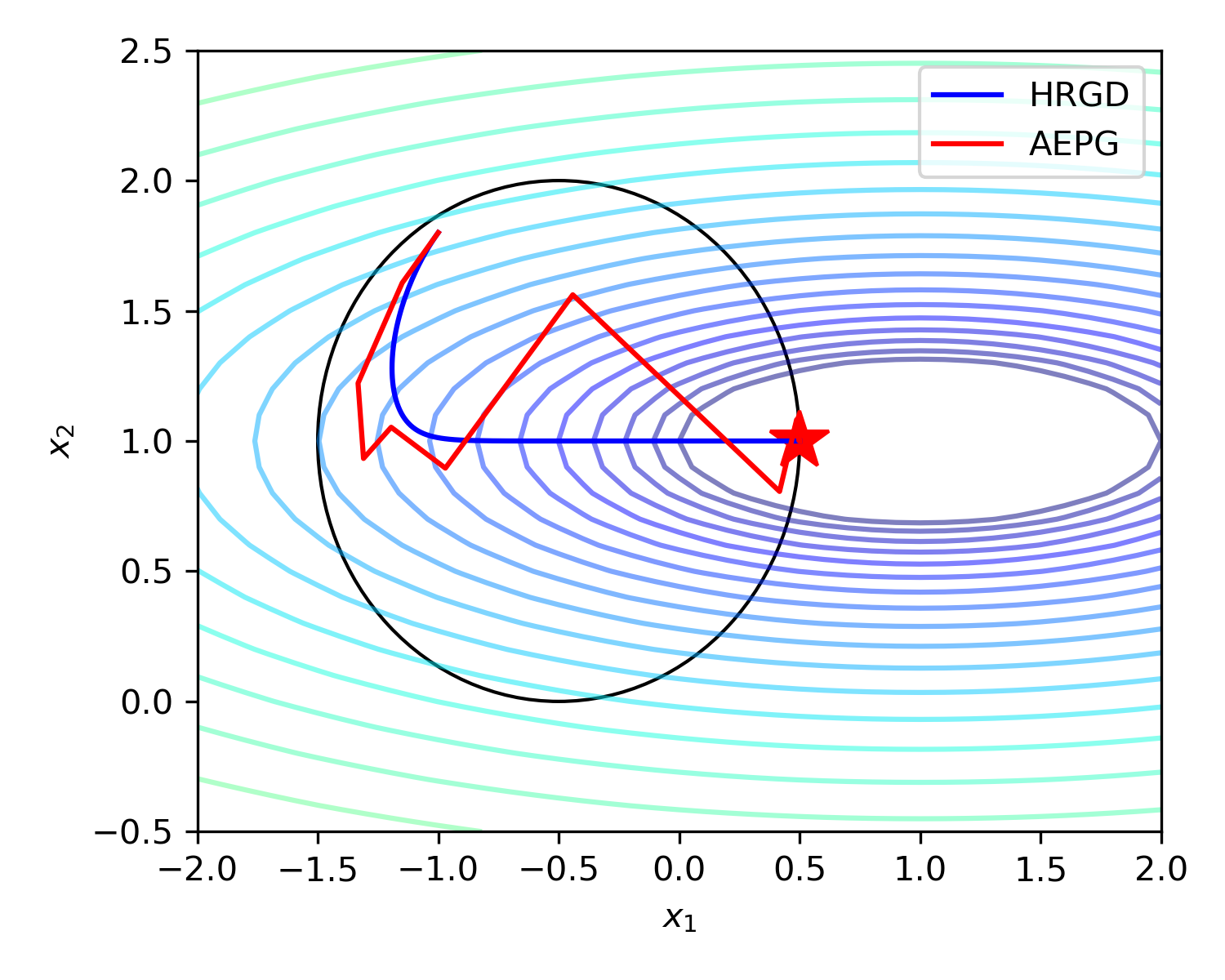
(a) Quadratic

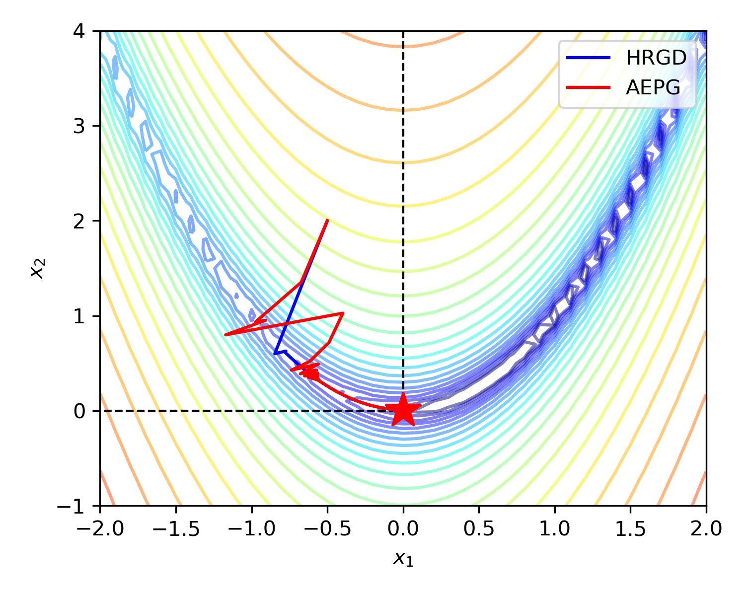
(b) Rosenbrock

Figure 1. Contour plot and trajectories of AEPG and HRGD on the constrained quadratic problem with $\alpha=10$ (a) and the constrained Rosenbrock problem with $\alpha=100$ (b). The red star in each plot represents the minimum point.

6.1.1. Convex objectives

We start with the following constrained quadratic problem:

$$\min\quad f(x_{1},x_{2})=(x_{1}-1)^{2}+\alpha(x_{2}-1)^{2},$$

s.t. $$(x_{1}+0.5)^{2}+(x_{2}-1)^{2}\leq 1,$$

where $\alpha$ is a positive constant. With the given constraint, the minimum value of $f$ is $0.25$ achieved at $(0.5,1)$. In our experiments, we vary the value of $\alpha$, which corresponds to the condition number of $\nabla^{2}f$, and solve the problems by HRGD (2.2) with $A=H(x)$, and AEPG (Algorithm 1) with $A^{\dagger}=H(x)^{-1}$. Here the Hessian matrix is defined by $H=\nabla^{2}h$, with

$$h(x_{1},x_{2})=u\ln u-u,\quad u:=u(x_{1},x_{2})=1-(x_{1}+0.5)^{2}-(x_{2}-1)^{2}.$$

The initial point is set at $(-1,1.8)$. The results are presented in Table 1, also shown in Figure 1 (a).

Table 1. Number of iterations of HRGD and AEPG to achieve $\epsilon$ accuracy on the constrained quadratic problem. Ratio = the number of iterations of HRGD / the number of iterations of AEPG.

$\alpha$	$\epsilon$	HRGD	AEPG	Ratio
1	1e-7	416	103	4
10	1e-6	3175	47	67
100	1e-5	23120	723	32
1000	1e-4	14190	1715	8
10000	1e-3	147284	5075	29

6.1.2. Nonconvex objectives

We then consider the benchmark 2D-Rosenbrock function of the form

$$f(x_{1},x_{2})=(x_{1}-1)^{2}+\alpha(x_{2}-x_{1}^{2})^{2},$$

where $\alpha$ is a positive constant. This is a standard test case for optimization algorithms. The global minimum $(1,1)$ is inside a long, narrow, parabolic flat valley. Finding the valley is simple, but finding the actual minimum of the function is less trivial. In this example, we test the constrained problem:

$$\min\quad f(x_{1},x_{2})=(x_{1}-1)^{2}+\alpha(x_{2}-x_{1}^{2})^{2},\quad\text{s.t. }\quad x_{1}<0,\;x_{2}>0.$$

With the given constraint, the minimum value of $f$ becomes $1$ at $(0,0)$. We vary the value of $\alpha$, which controls the condition number of $\nabla^{2}f$ and solve the problem by NGD with $A=H(x)$, and AEPG (Algorithm 1) with $A^{\dagger}=H(x)^{-1}$. Here the Hessian matrix is defined by $H=\nabla^{2}h$, with

$$h(x_{1},x_{2})=K(-x_{1})+K(x_{2}),\quad K(s)=s\ln s-s,$$

which leads to $A^{\dagger}=\text{diag}(-x_{1},x_{2})$. The initial point is set at $(-0.5,2)$. The results are presented in Table 2. Numerically, we observe that with a suitably larger step size, AEPG still converges to the minimum point, as shown in Figure 1 (b).

Table 2. Number of iterations of HRGD and AEPG to achieve $\epsilon$ accuracy on the constrained Rosenbrock problem. Here $\alpha$ controls the condition number of $\nabla^{2}f$; the stopping criteria is $|f(x)-f^{*}|<\epsilon$; Ratio = the number of iterations of HRGD / the number of iterations of AEPG.

$\alpha$	$\epsilon$	HRGD	AEPG	Ratio
1	1e-7	7896	4802	2
10	1e-6	7935	1563	4
100	1e-5	8712	1656	5
1000	1e-4	28705	1618	18
10000	1e-3	226524	3346	68

6.1.3. $D$-Optimal Design Problem

Consider the problem of estimating a vector $x\in\mathbb{R}^{m}$ from measurements $y\in\mathbb{R}^{n}$ given by the relationship

$$y=Ux+\delta,\quad\delta\sim\mathcal{N}(0,1),$$

where $U=[u_{1},\cdots,u_{n}]^{\top}$ is a matrix that contains $n$ test (column) vectors $u_{i}\in\mathbb{R}^{m}$. A reasonable goal during the design phase of an experiment is to minimize the covariance matrix, which is proportional to $(U^{\top}U)^{-1}$. With the D-optimality criteria, the problem can be written as a minimum determinant problem [42]:

$$\min_{\theta} L(\theta):=\log\det\left(\sum_{i=1}^{n}\theta_{i}u_{i}u_{i}^{\top}\right)^{-1},$$ (6.1)

s.t. $$\sum_{i=1}^{n}\theta_{i}=1\quad\text{and}\quad\theta_{i}\geq 0,\quad i\in[n].$$

This is a convex problem, with the unit simplex as feasible region. In computational geometry, the $D$-optimal design problem arises as a dual problem of the minimum volume covering ellipsoid (MVCE) problem, and is useful in various application areas, for example, computational statistics and data mining [42].

To apply AEPG (Algorithm 1) to solve (6.1), we define the Hessian matrix by $H=\nabla^{2}h$, with

$$h(\theta)=\sum_{i=1}^{n}K(\theta_{i}),\quad K(s)=s\ln s-s.$$

from which we have $H(\theta)^{-1}={\rm diag}(\theta_{1},...,\theta_{n})$. Also note that $B=[1,1,...,1]$, thus the preconditioning matrix defined by (3.7) has the form of

$$A^{\dagger}(\theta) =H^{-1}-H^{-1}B^{\top}(BH^{-1}B^{\top})^{-1}BH^{-1}$$ (6.2)

$$={\rm diag}(\theta_{1},\cdots,\theta_{n})-\theta\theta^{\top},$$

where $BH^{-1}B^{\top}=\sum_{i=1}^{n}\theta_{i}=1$ is used. From the form of the preconditioning matrix in (6.2), we see that the computation of AEPG is independent of $m$ (the dimension of the test vectors $u_{i}$). Hence, AEPG is well-suited for solving D-optimal design problems constructed by high-dimensional test vectors.

Several other algorithms have been proposed for solving (6.1), for instance, the interior point method and the Frank–Wolfe (FW) method [12]. The interior point method needs the second-order derivative of $f$, while the FW method is a first-order gradient method. To make the comparison more convincing, we also consider FW with away steps (FW-away), an effective strategy that improves the vanilla FW algorithm’s convergence speed and solution accuracy. For details on applying FW and FW-away to solve the D-optimal design problem, see [10, Chapter 5.2.7].

In our experiments, we fix $n=1000$ (number of test vectors), and compare AEPG (Algorithm 1) with the other algorithms when $m=10,30,50,80,100,200,300,400,500$. We generate test vectors $u_{i}$ using independent random Gaussian distributions with zero mean and unit variance. The initial point is set as $\theta_{0}=(\frac{1}{n},...,\frac{1}{n})$. All computation is done in Python 3.7 on a 2 GHz PC with 16 GB Memory.

Comparison with the interior point method (IPM). For cases where $m=10,30,50,80,100$, we compare AEPG with the IPM . Specifically, we set the stopping criteria as $|L(\theta)-L^{*}|<10^{-7}$ and compare the computation time needed for both methods to achieve the stopping criteria. The results are summarized in Table 3, which shows that the computation time of AEPG is much less than that of IPM, especially for relatively large $m$ ($m>10$).

Table 3. Comparison between computational time (seconds) of AEPG and IPM on the D-optimal design problem, using datasets with varying dimensions of test vectors $m$ and a fixed number of test vectors $n=1000$.

m	n	AEPG	IPM
10	1000	2.84	1.39
30	1000	2.93	6.15
50	1000	3.02	21.33
80	1000	2.63	112.92
100	1000	2.44	253.37

Comparison with the Frank-Wolfe (FW) method. For cases where $m=200,300,400,500$, the IPM failed to solve the problems, we compare AEPG with the FW method and FW-away method. The results are presented in Figure 2. In all cases, we see that the vanilla FW algorithm does not find solutions that meet the stopping criteria, and AEPG takes less time than FW-away to reach the minimum value when $m=300,400,500$.

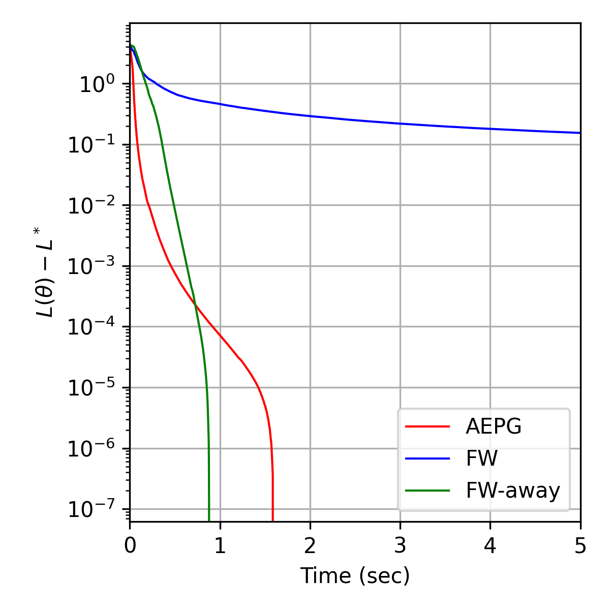
(a) $m=200$

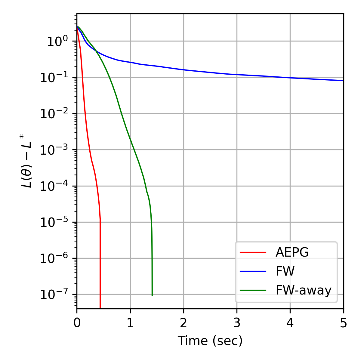
(b) $m=300$

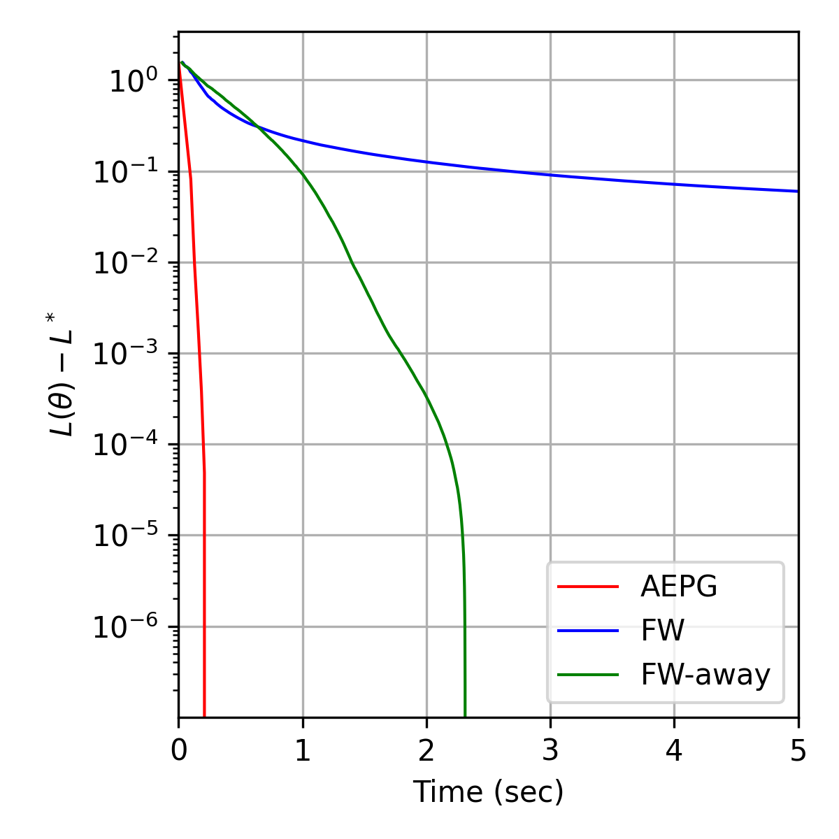
(c) $m=400$

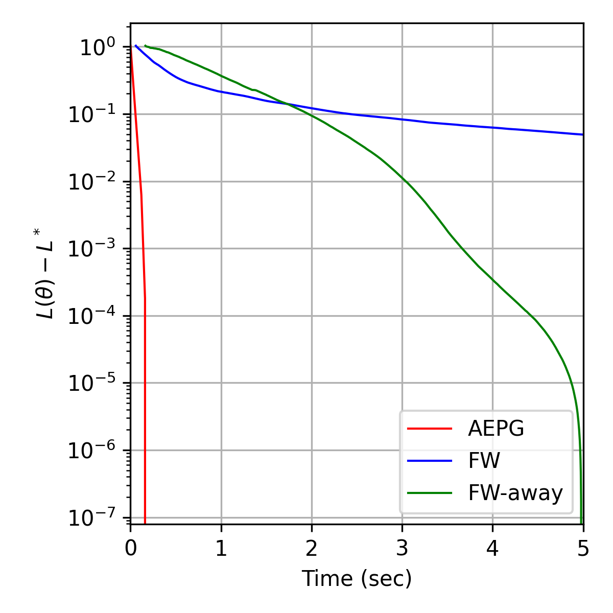
(d) $m=500$

Figure 2. Comparison between computational time (seconds) of AEPG and the FW/FW-away method on the D-optimal design problem, using datasets with varying dimensions of test vectors $m$ and a fixed number of test vectors $n=1000$

In both comparison experiments, we observe that unlike the FW-away algorithm and the IPM, whose computation time increases as $m$ gets larger, the computation time of AEPG is almost at the same level in all cases. The advantage of AEPG over the IPM and the FW-away algorithm becomes increasingly evident as $m$ gets larger.

6.2. Wasserstein natural gradient

Let $\rho$ be a 2-dimensional Gaussian mixture model given by

$$\rho(x;\theta)=w\mathcal{N}(x;(\theta_{1},3),I)+(1-w)\mathcal{N}(x;(\theta_{2},2),I),$$

where $w\geq 0$ is a weight factor. Following [32], we formulate the data fitting problem

$$\min_{\theta}\bigg{\{}L(\theta)=\frac{1}{2}\int_{\Omega}|\rho(x;\theta)-\rho^{*}(x)|^{2}dx\bigg{\}}.$$

Here, $\Omega$ is a compact domain, and $\rho^{*}(x)$ is the observed reference density function. In our experiments, we set $w=0.05$, $\Omega=[0,5]^{2}$, and $\rho^{*}(x)=\rho(x;(1,3))$. The initial point is set at $(4,4.2)$.

We apply the least-squares formulation (5.13) and (5.14) to compute the Wasserstein natural gradient and compare the performance of WNGD (2.2) and AEPG (Algorithm 1), the trajectories are present in Figure 3(b). We observe that both WNGD and AEPG are able to find the global minima and AEPG converges with fewer iterations. We also present the trajectories of GD and AEGD (using standard gradient) in Figure 3(a) and see that both methods with standard gradient got stuck at a local minimum.

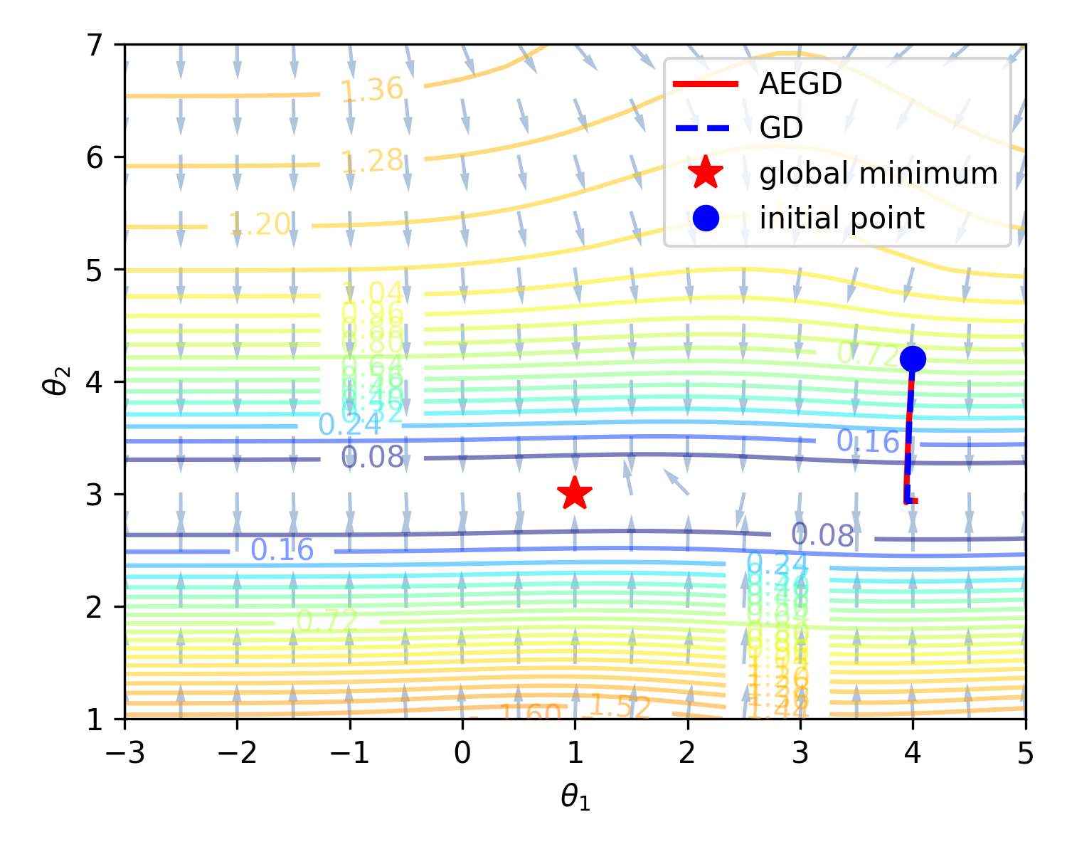
(a) Standard gradient

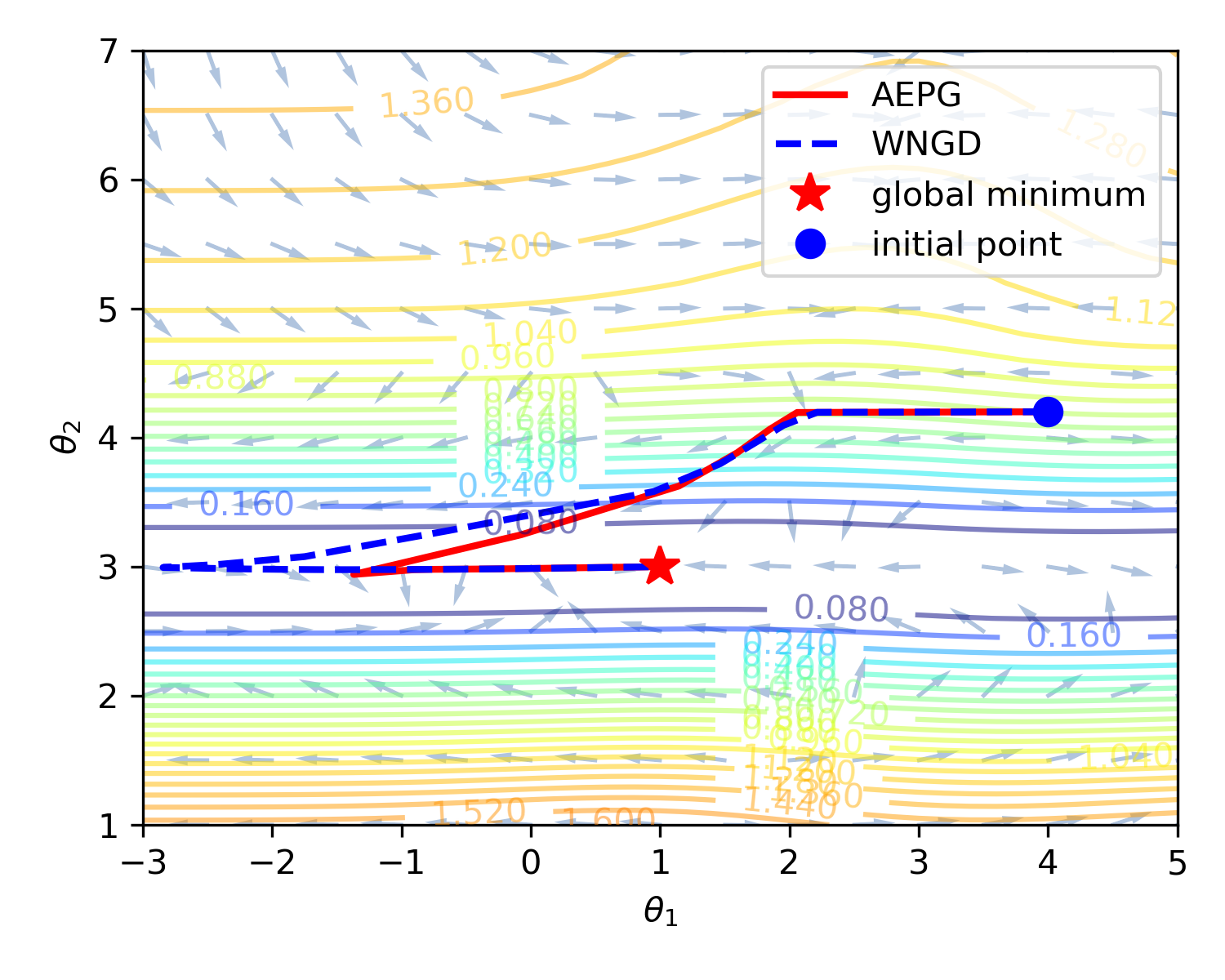
(b) Wasserstein natural gradient

Figure 3. Gaussian mixture model: level sets, vector fields, and convergent paths using (a) methods with standard gradient (b) methods with the Wasserstein natural gradient.

7. Discussion

This work proposes a unified framework to apply AEGD (Adaptive gradient method with energy) techniques based on a general preconditioning descent direction for solving constrained optimization problems. The key idea is to incorporate the benefits of both the descent direction adapting to the geometry of the problem and the step size being adjusted by an energy variable.

Theoretically, we show that AEPG is unconditionally energy stable, irrespective of step size. When the base step size is suitably small, we proved that AEPG is guaranteed to find a minimum value of the objective function. For the descent direction preconditioned by a positive definite matrix, we also derived the convergence rates for three types of objective functions: general differentiable functions, nonconvex functions that satisfy Polyak–Lojasiewic’s (PL) condition, and convex functions.

We investigate two application tasks where the optimization problem with explicit or implicit constraints. One application is the optimization problems with parameters in a convex set. We follow the strategy in [3], endowing the feasible set with a Riemannian metric so that AEPG is applicable. Extension to the case, also with a linear equality constraint, is done by adjusting the preconditioning matrix by a projection operator. We again establish convergence theories under a mild set of assumptions. Another application is the optimization problems over the probability density space with the Wasserstein metric. In order to compute the natural gradient $G(\theta)^{-1}\nabla L(\theta)$ in AEPG efficiently, we follow the strategy in [32] by converting the natural gradient as the solution to a least-squares problem.

Numerical results show that AEPG exhibits faster convergence when compared with NGD, especially on ill-conditioned or nonconvex problems. In particular, these results indicate that the choice of the preconditioning matrix not only can change the rate of convergence but also influence the stationary point where the iterates converge, given a nonconvex optimization landscape.

Most efficient choices of Riemannian metrics are unclear for manifolds with complicated structures. Good options should probably combine the characteristics of specific problems and applications. Indeed, identifying a proper preconditioning matrix yielding faster convergence without introducing a computational overhead is essential. Furthermore, efficient methods for computing the natural gradient for large-scale optimization problems are also critical.

Funding

This work has been partially supported by National Science Foundation (NSF) grants DMS1812666 and DMS2135470 to Hailiang Liu and Xuping Tian; Air Force Office of Scientific Research (AFOSR), Multi-University Research Initiative (MURI) FA 9550 18-1-0502 grant to Levon Nurbekyan, and National Science Foundation (NSF) grant DMS-1913129 to Yunan Yang.

Data Availability

The synthetic data supporting Table 3 and Figure 2 are included at https://github.com/txping/AEPG.

Declarations

Conflict of interest

The authors have no relevant financial or non-financial interests to disclose.

Appendix A Technical proofs

In this section, we prove some theoretical results stated in Section 2:

A.1. Proof of Theorem 2.4

To examine the convergence behavior of AEPG (1.3), we reformulate it as

$$\theta_{k+1}=\theta_{k}-\eta_{k}A_{k}^{-1}\nabla L(\theta_{k}),\quad\eta_{k}:=\eta\frac{r_{k+1}}{l(\theta_{k})}.$$ (A.1)

Using $\alpha$-smoothness of $L$, we have

$$L(\theta_{k+1}) =L(\theta_{k}-\eta_{k}A_{k}^{-1}\nabla L(\theta_{k}))$$ (A.2)

$$\leq L(\theta_{k})-\eta_{k}\nabla L(\theta_{k})^{\top}A_{k}^{-1}\nabla L(\theta_{k})+\frac{\eta^{2}_{k}\alpha}{2}\|A_{k}^{-1}\nabla L(\theta_{k})\|^{2}$$

$$\leq L(\theta_{k})-\eta_{k}\|\nabla L(\theta_{k})\|^{2}_{A^{-1}_{k}}+\frac{\eta^{2}_{k}\alpha}{2\lambda_{1}}\|\nabla L(\theta_{k})\|^{2}_{A^{-1}_{k}}$$

$$=L(\theta_{k})-\eta_{k}\left(1-\frac{\eta_{k}\alpha}{2\lambda_{1}}\right)\|\nabla L(\theta_{k})\|^{2}_{A^{-1}_{k}}.$$

This ensures that $L(\theta_{k})$ is strictly decreasing as long as $\|\nabla L(\theta_{k})\|^{2}_{A^{-1}_{k}}\neq 0$, providing that

$$0<\eta_{k}<\frac{2\lambda_{1}}{\alpha}.$$ (A.3)

Hence we have $L(\theta_{k})$ converges as $k\to\infty$. We further sum (A.2) over $k$ to get

$$\sum_{k=0}^{\infty}\eta_{k}\left(1-\frac{\eta_{k}\alpha}{2\lambda_{1}}\right)\|\nabla L(\theta_{k})\|^{2}_{A^{-1}_{k}}\leq\sum_{k=0}^{\infty}\left(L(\theta_{k})-L(\theta_{k+1})\right)\leq L(\theta_{0})-\inf L(\theta_{k})<\infty.$$

This implies

$$\lim_{k\to\infty}\eta_{k}\left(1-\frac{\eta_{k}\alpha}{2\lambda_{1}}\right)\|\nabla L(\theta_{k})\|^{2}_{A^{-1}_{k}}=0.$$ (A.4)

With $\eta\leq\eta_{s}$, Lemma 2.2 gaurantees that $\eta_{k}:=\eta\frac{r_{k+1}}{l(\theta_{k})}\geq\frac{\eta r^{*}}{l(\theta_{0})}$ when $r_{0}\geq\frac{L(\theta_{0})-L^{*}}{2l^{*}\lambda_{1}}$. With $\eta\leq\eta_{0}=\frac{\lambda_{1}l^{*}}{\alpha r_{0}}$, we have $\eta_{k}:=\eta\frac{r_{k+1}}{l(\theta_{k})}\leq\frac{\lambda_{1}}{\alpha}$. These two bounds imply that $\eta_{k}\left(1-\frac{\eta_{k}\alpha}{2\lambda_{1}}\right)\geq\frac{\eta r^{*}}{2l(\theta_{0})}>0$, which together with (A.4) ensures that $\|\nabla L(\theta_{k})\|^{2}_{A^{-1}_{k}}\to 0$, hence $\|\nabla L(\theta_{k})\|\to 0$ since $A^{-1}$ is positive definite. Therefore, $L(\theta_{k})$ is guaranteed to converge to a local minimum value of $L$.

A.2. Proof of Theorem 2.5

(ii) Using the $\alpha$-smoothness assumption and similar derivation as (A.2), we have

$$L(\theta_{k+1})-L(\theta_{k}) \leq-\eta_{k}\left(1-\frac{\eta_{k}\alpha}{2\lambda_{1}}\right)\|\nabla L(\theta_{k})\|^{2}_{A^{-1}_{k}}$$

$$\leq-\frac{\eta_{k}}{2}\|\nabla L(\theta_{k})\|^{2}_{A^{-1}_{k}}\quad\text{(since $\eta_{k}\leq\lambda_{1}/\alpha$)}$$

$$\leq-\frac{\eta_{k}}{2\lambda_{n}}\|\nabla L(\theta_{k})\|^{2}.$$ (A.5)

Denote $w_{k}=L(\theta_{k})-L(\theta^{*})$, then the PL property of function $L$ implies

$$\frac{1}{2}\|\nabla L(\theta_{k})\|^{2}\geq\mu(L(\theta_{k})-L(\theta^{*}))=\mu w_{k}.$$ (A.6)

With this property, (A.5) can be written as

$$w_{k+1}-w_{k}\leq-\frac{\mu\eta_{k}}{\lambda_{n}}w_{k}\quad\Rightarrow\quad w_{k+1}\leq\Big{(}1-\frac{\mu\eta_{k}}{\lambda_{n}}\Big{)}w_{k}.$$ (A.7)

By induction,

$$w_{k} \leq w_{0}\prod_{j=0}^{k-1}\Big{(}1-\frac{\mu\eta_{j}}{\lambda_{n}}\Big{)}=w_{0}\exp\left(\sum_{j=0}^{k-1}{\rm log}\Big{(}1-\frac{\mu\eta_{j}}{\lambda_{n}}\Big{)}\right)\leq w_{0}\exp\left(-\mu\sum_{j=0}^{k-1}\frac{\eta_{j}}{\lambda_{n}}\right).$$

Note for $j<k$ that $\eta_{j}=\eta\frac{r_{j+1}}{l(\theta_{j})}\geq\eta\frac{r_{k}}{l(\theta_{0})},$ hence,

$$w_{k}\leq W_{0}\exp\Big{(}-\frac{c_{0}kr_{k}}{\lambda_{n}}\Big{)},\quad c_{0}=\frac{\mu\eta}{l(\theta_{0})}.$$

To ensure convergence of $\theta_{k}$, we use $\alpha$-smoothness for $L$ and scheme (A.1) to get

$$L(\theta_{k+1})-L(\theta_{k}) \leq\nabla L(\theta_{k})^{\top}(\theta_{k+1}-\theta_{k})+\frac{\alpha}{2}\|\theta_{k+1}-\theta_{k}\|^{2}$$

$$\leq-\frac{1}{\eta_{k}}\|\theta_{k+1}-\theta_{k}\|^{2}_{A_{k}}+\frac{\alpha}{2}\|\theta_{k+1}-\theta_{k}\|^{2}$$

$$\leq(-\frac{\lambda_{1}}{\eta_{k}}+\frac{\alpha}{2})\|\theta_{k+1}-\theta_{k}\|^{2}$$

$$\leq-\frac{\lambda_{1}}{2\eta_{k}}\|\theta_{k+1}-\theta_{k}\|^{2}\quad\text{(since $\eta_{k}\leq\lambda_{1}/\alpha$)},$$

which further implies

$$w_{k}-w_{k+1}\geq\frac{\lambda_{1}}{2\eta_{k}}\|\theta_{k+1}-\theta_{k}\|^{2}.$$ (A.8)

The PL property (A.6) when combined with (A.1) gives

$$\|A_{k}(\theta_{k+1}-\theta_{k})\|^{2}=\eta^{2}_{k}\|\nabla L(\theta_{k})\|^{2}\geq 2\mu\eta^{2}_{k}w_{k}\quad\Rightarrow\quad\frac{1}{\sqrt{w_{k}}}\geq\frac{\sqrt{2\mu}\eta_{k}}{\lambda_{n}\|\theta_{k+1}-\theta_{k}\|}.$$ (A.9)

Using $w_{k}>w_{k+1}$, we have

$$\sqrt{w_{k}}-\sqrt{w_{k+1}} \geq\frac{1}{2\sqrt{w_{k}}}(w_{k}-w_{k+1})\geq\frac{\sqrt{2\mu}\lambda_{1}}{4\lambda_{n}}\|\theta_{k+1}-\theta_{k}\|.$$

Here the last inequality is by (A.8) and (A.9). Taking summation over $k$ gives

$$\sum_{k=0}^{\infty}\|\theta_{k+1}-\theta_{k}\|\leq\frac{4\lambda_{n}}{\sqrt{2\mu}\lambda_{1}}\sqrt{w_{0}}.$$

This yields (2.12), which ensures the convergence of $\{\theta_{k}\}$.

(iii) With the convexity assumption on $L$, we have

$$w_{k}:=L(\theta_{k})-L(\theta^{*}) \leq\nabla L(\theta_{k})^{\top}(\theta_{k}-\theta^{*})\leq\|\nabla L(\theta_{k})\|\|\theta_{k}-\theta^{*}\|,$$

where we used the Cauchy-Schwarz inequality. We claim that for convex $f$,

$$\|\theta_{k}-\theta^{*}\|\leq\|\theta_{0}-\theta^{*}\|.$$ (A.10)

The proof is defer to the end of this subsection. Thus we have

$$\|\nabla L(\theta_{k})\|\geq\frac{w_{k}}{\|\theta_{k}-\theta^{*}\|}\geq\frac{w_{k}}{\|\theta_{0}-\theta^{*}\|}.$$ (A.11)

This when combined with (A.5) (since $\eta_{k}\leq\lambda_{1}/\alpha$) leads to

$$w_{k+1}\leq w_{k}-\frac{\eta_{k}}{2\lambda_{n}\|\theta_{0}-\theta^{*}\|^{2}}w_{k}^{2}.$$ (A.12)

This implies $w_{k}\geq w_{k+1}$. Multiplying $\frac{1}{w_{k+1}w_{k}}$ on both sides gives

$$\frac{1}{w_{k}}\leq\frac{1}{w_{k+1}}-\frac{\eta_{k}}{2\lambda_{n}\|\theta_{0}-\theta^{*}\|^{2}}\frac{w_{k}}{w_{k+1}}\leq\frac{1}{w_{k+1}}-\frac{\eta_{k}}{2\lambda_{n}\|\theta_{0}-\theta^{*}\|^{2}}.$$

Using $\eta_{j}=\eta\frac{r_{j+1}}{l(\theta_{j})}\geq\eta\frac{r_{k}}{l(\theta_{0})}$, we proceed to obtain

$$\frac{1}{w_{k}} \geq\frac{1}{w_{k-1}}+\frac{\eta_{k-1}}{2\lambda_{n}\|\theta_{0}-\theta^{*}\|^{2}}$$

$$\geq\frac{1}{w_{0}}+\frac{1}{2\lambda_{n}\|\theta_{0}-\theta^{*}\|^{2}}\sum_{j=0}^{k-1}\eta_{j}$$

$$\geq\frac{k\eta r_{k}}{2\lambda_{n}l(\theta_{0})\|\theta_{0}-\theta^{*}\|^{2}}.$$

Hence for $\max_{j<k}\eta_{j}\leq\lambda_{1}/\alpha$, we have

$$L(\theta_{k})-L(\theta^{*})=w_{k}\leq\frac{c_{1}\lambda_{n}\|\theta_{0}-\theta^{*}\|^{2}}{kr_{k}},\quad c_{1}=\frac{2l(\theta_{0})}{\eta}.$$

Finally, we prove claim (A.10). We proceed with

$$\theta_{k+1}-\theta^{*} =\theta_{k}-\theta^{*}-\eta_{k}A_{k}^{-1}\nabla L(\theta_{k})$$

$$=\theta_{k}-\theta^{*}-\eta_{k}A_{k}^{-1}(\nabla L(\theta_{k})-\nabla L(\theta^{*}))$$

$$=\theta_{k}-\theta^{*}-\eta_{k}A_{k}^{-1}\left(\int_{0}^{1}\nabla^{2}L(\theta^{*}+s(\theta_{k}-\theta^{*}))ds=:B_{k}\right)(\theta_{k}-\theta^{*}).$$

Denote $d_{k}:=\|\theta_{k}-\theta^{*}\|$, we have

$$d_{k+1} =\|(I-\eta_{k}A_{k}^{-1}B_{k})(\theta_{k}-\theta^{*})\|$$

$$\leq\max_{0\leq\xi\leq\frac{\alpha}{\lambda_{1}}}|1-\eta_{k}\xi|d_{k}.$$

For $\eta_{k}\leq\lambda_{1}/\alpha$, we have

$$d_{k+1} \leq d_{k},$$

hence $d_{k}\leq d_{0}$ for any integer $k$. This completes the proof.

A.3. Proof of Theorem 2.9

(3) The proof is similar to the proof for Theorem 2.4. Using $\alpha$-smoothness, we have

$$L(\theta_{k+1}) =L(\theta_{k}-\eta_{k}A^{\dagger}_{k}\nabla L(\theta_{k}))$$ (A.13)

$$\leq L(\theta_{k})-\eta_{k}\nabla L(\theta_{k})^{\top}A^{\dagger}_{k}\nabla L(\theta_{k})+\frac{\eta^{2}_{k}\alpha}{2}\|A^{\dagger}_{k}\nabla L(\theta_{k})\|^{2}.$$

Since $A^{\dagger}_{k}=P_{k}G_{k}^{-1}=G_{k}^{-1}P_{k}^{\top}$, we have

$$L(\theta_{k+1}) \leq L(\theta_{k})-\eta_{k}\|P_{k}^{\top}\nabla L(\theta_{k})\|^{2}_{G_{k}^{-1}}+\frac{\alpha\eta_{k}^{2}}{2\lambda_{1}}\|P_{k}^{\top}\nabla L(\theta_{k})\|^{2}_{G_{k}^{-1}}$$

$$=L(\theta_{k})-\eta_{k}\left(1-\frac{\eta_{k}\alpha}{2\lambda_{1}}\right)\|P_{k}^{\top}\nabla L(\theta_{k})\|^{2}_{G_{k}^{-1}}.$$ (A.14)

This ensures that $L(\theta_{k})$ is strictly decreasing as long as $\|P_{k}^{\top}\nabla L(\theta_{k})\|^{2}_{G^{-1}_{k}}\neq 0$, providing that A.3 holds. For the rest of the proof, we refer the readers to A.1.

(4) We now turn to estimate convergence rates, while we use

$$\quad P_{k}=I-G_{k}^{-1}B^{\top}(BG_{k}^{-1}B^{\top})^{-1}B$$

so that $BP_{k}=0$.

(i) In the proof of (i) for Theorem 2.5, we replace $v_{k}=G^{-1}_{k}\nabla l(\theta_{k})$ by $G_{k}^{-1}P_{k}^{\top}\nabla l(\theta_{k})$, thus obtain the stated convergence bound for $\min_{j<k}\|P_{j}^{\top}\nabla L(\theta_{j})\|^{2}$.

(ii) We first show convergence of $\theta_{k}$. Using $\eta_{k}\leq\frac{\lambda_{1}}{\alpha}$, we further bound (A.3) by

$$L(\theta_{k+1})\leq L(\theta_{k})-\frac{\eta_{k}}{2}\|P_{k}^{\top}\nabla L(\theta_{k})\|^{2}_{G_{k}^{-1}}.$$ (A.15)

This and

$$\theta_{k+1}-\theta_{k}=-\eta_{k}G_{k}^{-1}P_{k}^{\top}\nabla L(\theta_{k})\in K,\quad K:=\{p|\quad Bp=0\}$$

lead to

$$L(\theta_{k+1})-L(\theta_{k})\leq-\frac{\lambda_{1}}{2\eta_{k}}\|\theta_{k+1}-\theta_{k}\|^{2}\quad\Rightarrow\quad w_{k}-w_{k+1}\geq\frac{\lambda_{1}}{2\eta_{k}}\|\theta_{k+1}-\theta_{k}\|^{2}.$$ (A.16)

The projected PL property (2.20) when combined with (A.16) gives

$$\|G_{k}(\theta_{k+1}-\theta_{k})\|^{2}=\eta^{2}_{k}\|P_{k}^{\top}\nabla L(\theta_{k})\|^{2}\geq 2\mu\eta^{2}_{k}w_{k}\quad\Rightarrow\quad\frac{1}{\sqrt{w_{k}}}\geq\frac{\sqrt{2\mu}\eta_{k}}{\lambda_{n}\|\theta_{k+1}-\theta_{k}\|}.$$ (A.17)

Combining (A.16) with (A.17) gives

$$\sqrt{w_{k}}-\sqrt{w_{k+1}}\geq\frac{1}{2\sqrt{w_{k}}}(w_{k}-w_{k+1})\geq\frac{\sqrt{2\mu}\lambda_{1}}{4\lambda_{n}}\|\theta_{k+1}-\theta_{k}\|.$$

This ensures that $\theta_{k}$ is a Cauchy sequence, hence $\theta_{k}\to\theta^{*}$ as $k\to\infty$.

Next we show the convergence rate of $w_{k}=L(\theta_{k})-L(\theta^{*})$. From (A.15) we have

$$w_{k+1}-w_{k}=L(\theta_{k+1})-L(\theta_{k})\leq-\frac{\eta_{k}}{2\lambda_{n}}\|P_{k}^{\top}\nabla L(\theta_{k})\|^{2}$$ (A.18)

for $\eta_{k}\leq\frac{\lambda_{1}}{\alpha}$. By the the projected PL condition (2.20), we have

$$\|P_{k}^{\top}\nabla L(\theta_{k})\|^{2}\geq 2\mu w_{k},$$

hence

$$w_{k+1}\leq w_{k}\Big{(}1-\frac{\mu\eta_{k}}{\lambda_{n}}\Big{)},$$

which is exactly (A.7), hence an induction argument will imply

$$w_{k}\leq w_{0}\exp\Big{(}-\frac{c_{0}kr_{k}}{\lambda_{n}}\Big{)},\quad c_{0}=\frac{\mu\eta}{l(\theta_{0})}.$$

(iii) For linear constraint $q(\theta)=B\theta-b$, we have $\theta_{k+1}-\theta_{k}\in K=\{p|\quad Bp=0\}$ with $B=\nabla q(\theta_{k})$, hence $\theta_{k}-\theta^{*}\in K=\{p|\quad Bp=0\}$. By the convexity of $L$,

$$w_{k}:=L(\theta_{k})-L(\theta^{*}) \leq\nabla L(\theta_{k})^{\top}(\theta_{k}-\theta^{*})$$

$$=\nabla L(\theta_{k})^{\top}P_{k}(\theta_{k}-\theta^{*})$$

$$=(P_{k}^{\top}\nabla L(\theta_{k}))^{\top}(\theta_{k}-\theta^{*})$$

$$\leq\|P_{k}^{\top}\nabla L(\theta_{k})\|\|\theta_{k}-\theta^{*}\|,$$

which implies

$$\|P_{k}^{\top}\nabla L(\theta_{k})\|\geq\frac{w_{k}}{\|\theta_{k}-\theta^{*}\|}\geq\frac{w_{k}}{\|\theta_{0}-\theta^{*}\|}.$$

This when combined with (A.18) gives

$$w_{k+1}-w_{k}\leq-\frac{\eta_{k}}{2\lambda_{n}}\|P_{k}^{\top}\nabla L(\theta_{k})\|^{2}\leq-\frac{\eta_{k}w_{k}^{2}}{2\lambda_{n}\|\theta_{0}-\theta^{*}\|^{2}}.$$

This is the same as (A.12), and the rest argument in the proof for Theorem 2.5 (iii) applies here.

Appendix B Construction of $h$

We now present a construction of $h$ for $\mathcal{M}$ when (3.1) holds with a smooth concave $U$. We simply put

$$h(\theta)=K(U(\theta)),\quad\theta\in\operatorname{int}(\mathcal{M}),$$

where $K:(0,\infty)\to\mathbb{R}$ is a smooth function. Note that

$$\nabla h(\theta)=K^{\prime}(U(\theta))\nabla U(\theta),$$ (B.1)

$$\nabla^{2}h(\theta)=K^{\prime\prime}(U(\theta))\nabla U(\theta)\otimes\nabla U(\theta)+K^{\prime}(U(\theta))\nabla^{2}U(\theta),$$

it is clear that $K$ should be chosen to satisfy the following:

1. $\lim_{s\to 0^{+}}K^{\prime}(s)=-\infty$,

2. $\forall s>0$, $K^{\prime\prime}(s)>0$,

3. $\forall s>0$, $K^{\prime}(s)<0$ when $U$ is not an affine function.

Two common choices for $K$ are $-\ln(s)$ and $s\ln(s)-s$. See [3] for other admissible choices.

Lemma B.1.

Let $K$ be chosen to satisfy (i)-(iii) above, the strict convexity of $h=K(U)$ can be ensured only if

$$\xi\cdot\nabla U(\theta)=0,~{}\xi^{T}\nabla^{2}U(\theta)\xi=0~{}\Longrightarrow~{}\xi=0,\quad\forall\theta\in\operatorname{int}(\mathcal{M}).$$ (B.2)

Proof.

Let $\theta\in\operatorname{int}(\mathcal{M})$, and $\xi\in\mathbb{R}^{n}$. Based on the properties of $K$, we have that

$$\xi^{T}\nabla^{2}h(\theta)\xi=K^{\prime\prime}(U(\theta))|\nabla U(\theta)\xi|^{2}+K^{\prime}(U(\theta))\xi^{T}\nabla^{2}U(\theta)\xi^{T}\geq 0.$$

Equality holds if and only if

$$\xi\cdot\nabla U(\theta)=0\quad\text{and}\;\;\xi^{T}\nabla^{2}U(\theta)\xi=0.$$

Hence (B.2) implies the strict convexity of $h$. ∎

Remark B.2.

When $K(U)$ does not satisfy (B.2), it suffices to add a correction term to make $h$ strictly convex in $\mathcal{M}$. For instance, for domain

$$\mathcal{M}=\{\theta\in\mathbb{R}^{n}\;|\;U_{i}(\theta)\geq 0,i\in[p]\}$$ (B.3)

with each $U_{i}$ being concave, we can take

$$h(\theta)=\sum_{i=1}^{p}K(U_{i}(\theta))+\tilde{h}(\theta),\quad\theta\in\mathcal{M},$$

where $\tilde{h}$ is added to ensure the strict convexity of $h$ in $\mathcal{M}$. For example, if $\tilde{h}$ is strictly convex, we have that

$$\begin{split}\xi^{T}\nabla^{2}h(\theta)\xi=&\sum_{i=1}^{p}\left(K^{\prime\prime}(U_{i}(\theta))|\nabla U_{i}(\theta)\xi|^{2}+K^{\prime}(U_{i}(\theta))\xi^{T}\nabla^{2}U_{i}(\theta)\xi^{T}\right)+\xi^{T}\nabla^{2}\tilde{h}(\theta)\xi\\ \geq&\xi^{T}\nabla^{2}\tilde{h}(\theta)\xi>0,\quad\forall\xi\neq 0.\end{split}$$

Non-strictly convex choices for $\tilde{h}$ are also possible as long as it yields a strongly convex $h$ in combination with $(U_{i})_{i=1}^{p}$.

Example B.3.

For concreteness, we consider several examples below.

1. ($U$ is strictly concave) For domain $\mathcal{M}=\{\theta\in\mathbb{R}^{n}\;|\;U(\theta)\geq 0\}$ with $U=1-\theta^{T}S\theta$, where $S$ symmetric and positive definite, we can take

   $$h(\theta)=K(1-\theta^{T}S\theta).$$ (B.4)

2. ($\nabla U$ spans the whole space $\mathbb{R}^{n}$) For domain $\mathcal{M}=\{\theta\in\mathbb{R}^{n}\;|\;a_{i}\leq\theta_{i},i\in[n]\},$ we can take

   $$h(\theta)=\sum_{i=1}^{n}K(\theta_{i}-a_{i}).$$ (B.5)

3. For domain $\mathcal{M}=\{\theta\in\mathbb{R}^{n}~{}|~{}a_{i}\leq\theta_{i},i\in[p]\}$, where $1\leq p<n$ then

   $$h(\theta)=\sum_{i=1}^{p}K(\theta_{i}-a_{i})+\frac{1}{2}\sum_{i=p+1}^{n}\theta_{i}^{2},$$ (B.6)

   is a valid choice.

Appendix C On the projected PL condition

For the constrained minimization problem:

$$\min\quad L(\theta)=\frac{1}{2}\left(\beta\theta_{1}^{2}+\alpha\theta_{2}^{2}\right)$$

s.t. $$q(\theta)=a\theta_{1}+b\theta_{2}-1=0,$$

where $ab\not=0,\alpha\geq\beta>0$. The minimum point of this problem is

$$\theta^{*}=\bigg{(}\frac{a\alpha}{a^{2}\alpha+b^{2}\beta},\frac{b\beta}{a^{2}\alpha+b^{2}\beta}\bigg{)}.$$

Using $\nabla q(\theta)=(a,b)$ and (2.19), we have the projection matrix

$$P=\frac{1}{a^{2}+b^{2}}\begin{pmatrix}b^{2}&-ab\\ -ab&a^{2}\end{pmatrix},$$

and the projected gradient

$$P^{\top}\nabla L(\theta)=\frac{b\beta\theta_{1}-a\alpha\theta_{2}}{a^{2}+b^{2}}(b,-a)^{\top}.$$

To verify the projected PL condition, we note that

$$\|P^{\top}\nabla L(\theta)\|^{2} =\frac{(b\beta\theta_{1}-a\alpha\theta_{2})^{2}}{a^{2}+b^{2}}$$

$$=\frac{1}{a^{2}+b^{2}}\bigg{(}(b\beta+\frac{a^{2}\alpha}{b})\theta_{1}-\frac{a\alpha}{b}\bigg{)}^{2}$$

$$=\frac{1}{(a^{2}+b^{2})b^{2}}\bigg{(}(b^{2}\beta+a^{2}\alpha)\theta_{1}-a\alpha\bigg{)}^{2}$$

$$=\frac{(b^{2}\beta+a^{2}\alpha)^{2}}{(a^{2}+b^{2})b^{2}}(\theta_{1}-\theta^{*}_{1})^{2},$$

where $\theta_{2}=(1-a\theta_{1})/b$ was used in the second equality. Also,

$$L(\theta)-L(\theta^{*}) =\frac{1}{2}(\beta\theta^{2}_{1}+\alpha\theta^{2}_{2})-\frac{1}{2}(\beta\theta^{*2}_{1}+\alpha\theta^{*2}_{2})$$

$$=\frac{1}{2}\beta(\theta^{2}_{1}-\theta^{*2}_{1})+\frac{1}{2}\alpha(\theta^{2}_{2}-\theta^{*2}_{2})$$

$$=\frac{1}{2}\beta(\theta^{2}_{1}-\theta^{*2}_{1})+\frac{1}{2}\alpha\bigg{(}(\frac{1-a\theta_{1}}{b})^{2}-(\frac{1-a\theta^{*}_{1}}{b})^{2}\bigg{)}$$

$$=\bigg{(}\frac{1}{2}\beta+\frac{1}{2}\alpha\frac{a^{2}}{b^{2}}\bigg{)}(\theta^{2}_{1}-\theta^{*2}_{1})-\frac{a\alpha}{b^{2}}(\theta_{1}-\theta^{*}_{1})$$

$$=\frac{a^{2}\alpha+b^{2}\beta}{2b^{2}}(\theta_{1}-\theta^{*}_{1})\bigg{(}(\theta_{1}+\theta^{*}_{1})-\frac{2a\alpha}{a^{2}\alpha+b^{2}\beta}\bigg{)}$$

$$=\frac{a^{2}\alpha+b^{2}\beta}{2b^{2}}(\theta_{1}-\theta^{*}_{1})^{2}.$$

Hence the projected PL condition holds for $\mu>0$ if

$$\mu\leq\frac{a^{2}\alpha+b^{2}\beta}{a^{2}+b^{2}}.$$

References

- [1] P-A Absil, Robert Mahony, and Rodolphe Sepulchre, Optimization algorithms on matrix manifolds, Princeton University Press, 2008.
- [2] Zeyuan Allen-Zhu, Katyusha: The first direct acceleration of stochastic gradient methods, Proceedings of the 49th Annual ACM SIGACT Symposium on Theory of Computing, 2017, pp. 1200–1205.
- [3] Felipe Alvarez, Jérôme Bolte, and Olivier Brahic, Hessian Riemannian gradient flows in convex programming, SIAM journal on control and optimization 43 (2004), no. 2, 477–501.
- [4] Shun-Ichi Amari, Natural gradient works efficiently in learning, Neural computation 10 (1998), no. 2, 251–276.
- [5] Michael Arbel, Arthur Gretton, Wuchen Li, and Guido Montúfar, Kernelized Wasserstein natural gradient, arXiv preprint arXiv:1910.09652 (2019).
- [6] Jonathan Barzilai and Jonathan M Borwein, Two-point step size gradient methods, IMA journal of numerical analysis 8 (1988), no. 1, 141–148.
- [7] Dimitri P Bertsekas, Constrained optimization and Lagrange multiplier methods, Academic press, 2014.
- [8] Silvere Bonnabel, Stochastic gradient descent on Riemannian manifolds, IEEE Transactions on Automatic Control 58 (2013), no. 9, 2217–2229.
- [9] Léon Bottou, Stochastic gradient descent tricks, Neural Networks: Tricks of the Trade: Second Edition, 2012, pp. 421–436.
- [10] Gábor Braun, Alejandro Carderera, Cyrille W Combettes, Hamed Hassani, Amin Karbasi, Aryan Mokhtari, and Sebastian Pokutta, Conditional gradient methods, arXiv preprint arXiv:2211.14103 (2022).
- [11] Yifan Chen and Wuchen Li, Optimal transport natural gradient for statistical manifolds with continuous sample space, Information Geometry 3 (2020), no. 1, 1–32.
- [12] S Damla Ahipasaoglu, Peng Sun, and Michael J Todd, Linear convergence of a modified Frank–Wolfe algorithm for computing minimum-volume enclosing ellipsoids, Optimisation Methods and Software 23 (2008), no. 1, 5–19.
- [13] Timothy Dozat, Incorporating Nesterov Momentum into Adam, Proceedings of the 4th International Conference on Learning Representations, 2016, pp. 1–4.
- [14] John Duchi, Elad Hazan, and Yoram Singer, Adaptive subgradient methods for online learning and stochastic optimization., Journal of machine learning research 12 (2011), no. 7.
- [15] Daniel Gabay, Minimizing a differentiable function over a differential manifold, Journal of Optimization Theory and Applications 37 (1982), 177–219.
- [16] Jiang Hu, Andre Milzarek, Zaiwen Wen, and Yaxiang Yuan, Adaptive quadratically regularized Newton method for Riemannian optimization, SIAM Journal on Matrix Analysis and Applications 39 (2018), no. 3, 1181–1207.
- [17] Diederik P Kingma and Jimmy Ba, Adam: A method for stochastic optimization, Proceedings of the 3th International Conference on Learning Representations, 2015.
- [18] Wuchen Li, Alex Tong Lin, and Guido Montúfar, Affine natural proximal learning, Geometric Science of Information: 4th International Conference, GSI 2019, Toulouse, France, August 27–29, 2019, Proceedings 4, Springer, 2019, pp. 705–714.
- [19] Wuchen Li and Guido Montúfar, Natural gradient via optimal transport, Information Geometry 1 (2018), 181–214.
- [20] Wuchen Li and Jiaxi Zhao, Wasserstein information matrix, Information Geometry (2023), 1–53.
- [21] Changshuo Liu and Nicolas Boumal, Simple algorithms for optimization on Riemannian manifolds with constraints, Applied Mathematics & Optimization 82 (2020), 949–981.
- [22] Hailiang Liu and Xuping Tian, An adaptive gradient method with energy and momentum, Ann. Appl. Math 38 (2022), no. 2, 183–222.
- [23] by same author, AEGD: adaptive gradient descent with energy, Numerical Algebra, Control and Optimization (2023).
- [24] Liyuan Liu, Haoming Jiang, Pengcheng He, Weizhu Chen, Xiaodong Liu, Jianfeng Gao, and Jiawei Han, On the variance of the adaptive learning rate and beyond, Proceedings of the 8th International Conference on Learning Representations, 2020.
- [25] Liangchen Luo, Yuanhao Xiong, Yan Liu, and Xu Sun, Adaptive gradient methods with dynamic bound of learning rate, Proceedings of the 7th International Conference on Learning Representations, 2019.
- [26] Anton Mallasto, Tom Dela Haije, and Aasa Feragen, A formalization of the natural gradient method for general similarity measures, Geometric Science of Information: 4th International Conference, GSI 2019, Toulouse, France, August 27–29, 2019, Proceedings 4, Springer, 2019, pp. 599–607.
- [27] James Martens, New insights and perspectives on the natural gradient method, The Journal of Machine Learning Research 21 (2020), no. 1, 5776–5851.
- [28] Yurii Nesterov, A method of solving a convex programming problem with convergence rate , Doklady Akademii Nauk, vol. 269, 1983, pp. 543–547.
- [29] by same author, Introductory lectures on convex optimization: A basic course, vol. 87, Springer Science & Business Media, 2003.
- [30] Yurii Nesterov, Alexander Gasnikov, Sergey Guminov, and Pavel Dvurechensky, Primal–dual accelerated gradient methods with small-dimensional relaxation oracle, Optimization Methods and Software 36 (2021), no. 4, 773–810.
- [31] Jorge Nocedal and Stephen J. Wright, Numerical optimization, Springer, 2006.
- [32] Levon Nurbekyan, Wanzhou Lei, and Yunan Yang, Efficient natural gradient descent methods for large-scale PDE-based optimization problems, SIAM Journal on Scientific Computing 45 (2023), no. 4, A1621–A1655.
- [33] Stanley Osher, Bao Wang, Penghang Yin, Xiyang Luo, Farzin Barekat, Minh Pham, and Alex Lin, Laplacian smoothing gradient descent, Research in the Mathematical Sciences 9 (2022), no. 3, 55.
- [34] Boris T Polyak, Some methods of speeding up the convergence of iteration methods, Ussr computational mathematics and mathematical physics 4 (1964), no. 5, 1–17.
- [35] by same author, Introduction to optimization, (1987).
- [36] Sashank J Reddi, Satyen Kale, and Sanjiv Kumar, On the convergence of Adam and beyond, Proceedings of the 7th International Conference on Learning Representations, 2019.
- [37] Guillaume Sagnol and Maximilian Stahlberg, PICOS: A Python interface to conic optimization solvers, Journal of Open Source Software 7 (2022), no. 70, 3915.
- [38] A Shapiro and Y Wardi, Convergence analysis of gradient descent stochastic algorithms, Journal of optimization theory and applications 91 (1996), 439–454.
- [39] Zebang Shen, Zhenfu Wang, Alejandro Ribeiro, and Hamed Hassani, Sinkhorn natural gradient for generative models, Advances in Neural Information Processing Systems 33 (2020), 1646–1656.
- [40] Ilya Sutskever, James Martens, George Dahl, and Geoffrey Hinton, On the importance of initialization and momentum in deep learning, Proceedings of the 30th International Conference on Machine Learning, 2013, pp. 1139–1147.
- [41] Tijmen Tieleman and Geoffrey Hinton, Lecture 6.5-RMSProp: Divide the gradient by a running average of its recent magnitude, COURSERA: Neural networks for machine learning 4 (2012), 26–31.
- [42] Lieven Vandenberghe, Stephen Boyd, and Shao-Po Wu, Determinant maximization with linear matrix inequality constraints, SIAM journal on matrix analysis and applications 19 (1998), no. 2, 499–533.
- [43] Cédric Villani, Topics in optimal transportation, vol. 58, American Mathematical Soc., 2021.
- [44] Xiaoxia Wu, Simon S Du, and Rachel Ward, Global convergence of adaptive gradient methods for an over-parameterized neural network, arXiv preprint arXiv:1902.07111 (2019).
- [45] Lexing Ying, Natural gradient for combined loss using wavelets, Journal of Scientific Computing 86 (2021), no. 2, 1–10.
- [46] Hongchao Zhang and William W Hager, A nonmonotone line search technique and its application to unconstrained optimization, SIAM journal on Optimization 14 (2004), no. 4, 1043–1056.
- [47] Juntang Zhuang, Tommy Tang, Yifan Ding, Sekhar C Tatikonda, Nicha Dvornek, Xenophon Papademetris, and James Duncan, Adabelief optimizer: Adapting stepsizes by the belief in observed gradients, Advances in neural information processing systems 33 (2020), 18795–18806.