MARES: A macroscopic approach to the radar echo scatter from high-energy particle cascades

Abstract

In this work, we provide a macroscopic model to predict the radar echo signatures found when a radio signal is reflected from a cosmic-ray or neutrino-induced particle cascade propagating in a dense medium like ice. Its macroscopic nature allows for an energy independent runtime, taking less than 10 s for simulating a single scatter event. As a first application, we discuss basic signal properties and simulate the expected signal for the T-576 beam-test experiment at the Stanford Linear Accelerator Center (SLAC). We find good signal strength agreement with the only observed radar echo from a high-energy particle cascade to date.

I Introduction

The discovery of the cosmic neutrino flux by the IceCube collaboration in 2013 established neutrino astronomy as a new window on the universe [1]. The IceCube experiment covers a volume of roughly 1 km³ instrumented with optical Cherenkov detectors to probe the remnants of the neutrino-ice interaction. The instrumentation of this volume allows the detection of cosmic neutrinos in the TeV-PeV energy range, but due to the steeply falling neutrino flux, IceCube runs low in statistics above PeV energies [2]. As such, detecting the cosmic neutrino flux above PeV energies, requires probing larger volumes than the 1 km³ that is currently monitored by IceCube. Radio waves travel roughly ten times further than optical signals in ice [3, 4], and are therefore a promising probe for instrumenting such larger detection volumes. As such, passive radio detection of high-energy particle cascades in dense media has been widely explored by the so-called Askaryan radio detectors [5]. The emission mechanism is coherent Cherenkov emission due to the net negative excess charge that builds up in the relativistic cascade as it propagates in the medium [6]. Its feasibility was shown in the laboratory [7], as well as in the radio detection of cosmic ray air showers [8, 9], but to date no neutrino-induced particle cascade has been identified. In this work, we discuss active radio detection of high-energy cosmic-ray or neutrino-induced particle cascades in dense media through the radar echo technique. Using a radio transmitter, a volume is constantly illuminated with radio waves. When a cosmic-ray or neutrino-induced particle cascade traverses the volume, the radio waves reflect off of the ionization plasma left in its wake. The reflection can subsequently be observed using a radio receiver. The earliest attempts date from the 1940s, when Blackett and Lovell theorized that the method may be suitable for the in-air detection of cosmic-ray air showers [10]. Concurrently, in 1941, Eckersley showed that a crucial component in earlier radar scatter modeling efforts was missing: the collisional damping of the free ionization charges responsible for the possible scatter [11]. As will be shown in Section 2, the main effect of this is that the plasma constituents, the free ionization charges, need to be treated as a collection of individual scattering objects, rather than a perfect coherent reflector over the plasma surface.

In spite of the calculation by Eckersley, several attempts were still made over the years to probe cosmic-ray air showers [11, 12], with a revival of the method in the early 2000s [13]. However, further theoretical advancements [14, 15], as well as limits obtained by the TARA experiment [16], finally deemed the radar echo method insufficient to probe cosmic-ray air showers.

Around the same time $(2010-2015)$, it was realized that cascades in dense media provide much more favorable detection properties. The main advantage is found in the drastic increase of the ionization plasma density left in the wake of the cascade [17, 18]. This triggered several experimental efforts to probe particle cascades propagating in dense media in the laboratory [19, 20], leading to the successful radar detection of such a cascade at the SLAC T-576 experiment [21] by the Radar Echo Telescope (RET) collaboration.

This successful detection initiated the Radar Echo Telescope for Cosmic Rays (RET-CR) experiment. Its goal is to probe the in-ice continuation of cosmic-ray air shower cores penetrating a high altitude ice sheet [22, 23]. RET-CR uses a cosmic-ray surface detector located on top of the ice sheet to trigger an in-ice radar detector. The in-ice detector aims to detect the continuation of the cosmic-ray particle cascade into the ice. As such, detecting this signal will show the in-nature proof-of-concept of the radar echo method to probe in-ice particle cascades. After the RET-CR experiment, the final goal of the RET collaboration is to perform neutrino astronomy using the radar echo telescope for neutrinos (RET-N) [24].

Although several modeling efforts for scattering radio waves off of in-air particle cascades have been developed [13, 25, 14, 15], currently the only available model to simulate the radar echo process from relativistic particle cascades in dense media is RadioScatter [26]. RadioScatter provides a particle level simulation of scattering from ionization deposits, which can be generated by, for example, the GEANT4 [27] toolkit.

In this work, we present a complementary, deterministic, modeling approach called MARES, a Macroscopic Approach to the Radar Echo Scatter. MARES provides an analytic, macroscopic treatment of the radar echo problem. The simulation code is written in c++ and designed to provide significant speedups in simulation time relative to existing particle level codes [26], which have energy-dependent runtime.

We first outline the scattering formalism by introducing the radar cross-section (RCS) for a macroscopic volume of coherent scatterers. Subsequently, the approach is extended to cover the full cascade, including its relativistic propagation, the latter leading to a non-trivial cascade RCS. As a first application, we discuss basic signal scattering properties and apply our model to the T-576 experiment at SLAC, showing good agreement with the observed signal.

II Radar scattering from a macroscopic volume of charges

The object we intend to detect is the ionization trail left in the wake of a relativistically moving particle cascade. Therefore, it is crucial to work at the electric field level, such that we are able to trace the phase information and determine the interference between different emission points within the plasma. As such, starting from the radar range equation, we first derive its electric field equivalent to obtain the field amplitude at the scattering point, which is subsequently re-emitted to the receiver. The signal phase and amplitude are traced independently.

The base of our calculation is initially found in the radar range equation [28]. This allows us to predict the scatter from a static macroscopic target having a radar scatter cross-section $\sigma_{RCS}$,

$$\begin{split}P_{R}&=P_{T}\frac{G_{T}G_{R}\lambda^{2}}{(4\pi)^{3}(R_{T}R_{R})^{2}}\sigma_{RCS},\end{split}$$ (1)

where the received power, $P_{R}$, is a function of the transmitted power, $P_{T}$; the gain of the transmitter and receiver antennas, $G_{T}$ and $G_{R}$; the distances of both antennas to the scattering element, $R_{T},R_{R}$; and the wavelength, $\lambda$, of the radio wave.

Using the medium impedance, for this work taken to be ice, $Z_{ice}$, and the antenna effective area $A_{R}=\left(\frac{\lambda^{2}G_{R}}{4\pi}\right)$  [28], the received power is related to the electric field amplitude $|E_{R}|$,

$$P_{R} =\frac{E_{R}^{2}}{2Z_{ice}}A_{R},$$ (2)

$$|E_{R}| =\sqrt{2Z_{ice}P_{R}\left(\frac{\ 4\pi}{\lambda^{2}G_{R}}\right)}.$$ (3)

This now allows us to re-write Eq. 1 in terms of the received electric field amplitude,

$$|E_{R}|=\frac{1}{4\pi R_{T}R_{R}}\sqrt{2Z_{ice}P_{T}G_{T}}\sqrt{\sigma_{RCS}}.$$ (4)

II.1 The damped electron radar cross-section

The scattering object under consideration in this work is the ionization plasma left in the wake of a high-energy particle cascade in ice. The calculations reported here are based on a model of the medium dominated by a damping rate parameter of $\omega_{c}/(2\pi)=\nu_{c}\approx 100\;\pm\;50$ THz. The order of magnitude is consistent with collision rates of electrons in ice, as derived in [26] and consistent with the electron mobility results found in [29]. In this model $\omega_{c}$ is much larger than the typical radio frequencies in the MHz-GHz range at which we aim to probe the plasma.

As such, the plasma is treated as a collection of individual scattering objects, oscillating in the incoming field, with the oscillation being strongly damped by collisions with the medium particles.

An emitter with transmit power $P_{T}$ and gain $G_{T}$ induces an electric field at the single charge equal to,

$$|E_{e}|=\sqrt{\frac{2Z_{ice}P_{T}G_{T}}{4\pi R_{T}^{2}}}.$$ (5)

For an incoming plane wave, the equation of motion for a single free charge in the plasma volume is properly modeled as a damped-driven oscillator with no natural frequency ($\omega_{0}=0$, free particle). Defining the collisional ratio,

$$W=\left(\frac{1}{\omega^{2}-i\omega\omega_{c}}\right),$$ (6)

the amplitude of the oscillation is found to be [30],

$$|x_{e}|=\frac{qE_{e}}{m}\left(\frac{1}{\omega^{2}-i\omega\omega_{c}}\right)=\frac{qE_{e}}{m}W=A_{0}W,$$ (7)

which is driven by the electric field at the scattering location $E_{e}$. The amplitude can be written in terms of the collision-less amplitude $A_{0}=qE_{e}m^{-1}$ that is damped by the collisional ratio, $W$. Here $q$ and $m$ respectively denote the charge and mass of the oscillator.

Having solved the equation of motion for the scatter, we obtain the scattered electric field at an arbitrary observer location through the standard field equations,

$$\vec{E}_{e,R} = \frac{q}{(4\pi\epsilon_{0})c^{2}R_{R}}[\hat{n}\times(\hat{n}\times\hat{\ddot{x}}_{e})]$$ (8)

$$= \frac{|E_{e}|(\omega^{2}W)}{R_{R}}\left(\frac{\sigma_{Th}G_{Hz}}{4\pi}\right)^{1/2}\;\;\hat{p}.$$

Here $\hat{n}$ denotes the unit vector pointing from the charge to the receiver. The final expression is written in terms of the Thomson scattering cross-section $\sigma_{Th}=\frac{8\pi}{3}r_{e}^{2}$, for which all constants sum to the classical electron radius $r_{e}\sim 2.8\cdot 10^{-15}$ m, and the Hertzian dipole gain factor $G_{Hz}~{}=\frac{3}{2}\sin^{2}(\theta)$ originating from the cross-product in the numerator of Eq. 8. The field is oscillating in the $\hat{p}$ direction given by the polarization of the incoming wave.

Eq. 4, now allows us to identify the radar scattering cross-section of the damped free electron:

$$\sigma_{RCS,e}=(\omega^{2}W)^{2}\sigma_{Th}G_{Hz}.$$ (9)

II.2 Scattering from a macroscopic volume

In this work, we construct our model based on the scatter off of $M$ coherent segments each containing a collection of $N_{i}$, $i=1,..,M$, scatterers. The geometry of this setup is outlined in Fig. 1. In order for a segment to satisfy the coherence condition, the dimensions of its scattering volume $d_{x},d_{y},d_{z}$ have to be much smaller than the relevant dimensions in the system. The relevant dimensions are given by the transmitter-cascade distance, $R_{T}$; the cascade-receiver distance, $R_{R}$ and the wavelength at which the plasma is probed, $\lambda_{T}$. As such, we require $d_{x},d_{y},d_{z}\ll R_{T},R_{R},\lambda_{T}$. Using this condition, the electric fields of the $N_{i}$ individual electrons within a segment will add constructively at our receiver.

The received power under coherence scales as $N_{i}^{2}$, hence the scatter from a single segment is given by,

$$P_{R,i}\propto|\vec{E}_{R,i}(R_{i},t)|^{2}=|N_{i}{E}_{e,R_{i}}(R_{i},t)|^{2},$$ (10)

with $E_{e,R_{i}}$ the scattered field from a single electron given by Eq. 8.

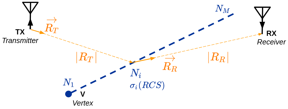
Figure 1: Basic diagram of the radar scatter of a line of scattering centers (segments).

II.3 Energy balance

We obtained the radar scatter from a macroscopic volume containing $N_{i}$ free electrons starting from a microscopic, single particle approach. The scattering off the individual particles attenuates the incoming wave. To calculate the response of multiple segments, we have to consider that part of the incoming wave energy is scattered away before reaching a following segment along its direction of propagation. The energy taken from the incoming wave by a single electron and which is re-scattered is [30]:

$$\left<P(t)\right>=\left<{F}(t)\dot{x}_{e}\right>=\frac{1}{2m}(qE_{0}\omega W)^{2}\omega_{c}.$$ (11)

For a volume $V$ containing $N$ electrons with electron number density $n_{e}$, the power density $\mathcal{P}=\frac{P}{V}=\left<P(t)\right>n_{e}$ is:

$$\mathcal{P}_{loss}=\frac{1}{2}\epsilon_{0}(\omega_{p}E_{0}\omega W)^{2}\omega_{c}$$ (12)

where $\omega_{p}=2\pi\nu_{p}$ is the angular plasma frequency,

$$\nu_{p}=\left(\frac{n_{e}q^{2}}{m\epsilon_{0}}\right)^{1/2}\approx 8980\sqrt{n_{e}\;[\mathrm{g/cm^{3}}]}.$$ (13)

Using the irradiance $I=\frac{\epsilon_{0}c}{2}E_{0}^{2}$, and attenuation of the incoming radio wave, $\beta=\frac{\omega_{c}}{c}(\omega\omega_{p}W)^{2}$, we can now identify $\mathcal{P}_{loss}=I\beta$.

Having obtained the power density taken from the incoming wave based on the microscopic approach outlined above, in the following we show this can also be obtained from pure macroscopic quantities. Following [26, 31], the macroscopic approach is based on the change in index of refraction, $n$, of the volume $V$ under consideration. Using this macroscopic point of view, the radar echo originates from the polarization of the medium upon an incoming electromagnetic wave and its subsequent de-excitation.

In the plasma under our consideration, $\mu=\mu_{0}$ and $\epsilon=\epsilon_{0}(1+\chi_{e})$ and therefore, the dispersion relation for the propagation of an incoming electromagnetic wave becomes, to good approximation ([31]):

$$k =\frac{\omega}{c}\left[1+\omega_{p}^{2}W\right]^{1/2}\simeq\frac{\omega}{c}\left[1+\frac{1}{2}\omega_{p}^{2}W\right]$$ (14)

$$=\mathrm{Re}(k)+i\;\mathrm{Im}(k).$$

The propagating radio wave ($\vec{k}$) gains an imaginary term, the plasma attenuation, $\beta$:

$$\beta =2\;\mathrm{Im}(k)=2\frac{\omega}{c}\;\mathrm{Im}(n)\simeq\frac{\omega}{c}\omega_{p}^{2}\;\mathrm{Im}(W)$$ (15)

$$=\frac{\omega_{c}}{c}(\omega\omega_{p}W)^{2}.$$

The attenuation of the radio waves considered along a path is the radio transparency, $\mathcal{T}$ :

$$P(z)=P_{0}e^{\int_{0}^{z}-\beta(l)dl}=P_{0}\mathcal{T}.$$ (16)

The attenuation of a radio wave going through a plasma volume $V$ of thickness $l$ and area $A$ can now be obtained as,

$$\mathcal{P}_{att} =\frac{\Delta P}{V}=\frac{1}{V}P_{0}(1-\mathcal{T})$$ (17)

$$=\frac{IA}{Al}(1-e^{-\beta l})\approx\frac{I}{l}\beta l=I\beta.$$

Here we used that in our case of interest, the over-damped regime ($\omega,\omega_{p}\ll\omega_{c}$), $\beta=\frac{\omega_{p}^{2}}{c\ \omega_{c}}$ becomes small. It follows that our plasma is indeed well described by the damped driven oscillator model, and the energy balance is obtained from both microscopic and macroscopic considerations. This also implies that the plasma needs to be treated as a collection of individual scattering objects oscillating and re-emitting in the incoming field, contrary to the so-called overdense regime ($\omega,\omega_{c}\ll\omega_{p}$), where the plasma would act as a perfect reflector scattering over its macroscopic surface.

III The particle cascade

We now apply the formalism developed in the previous section to the ionization plasma left in the wake of our particle cascade. To do so, we need a model of our plasma. For this, we first consider the relativistic particle cascade itself. Its longitudinal profile is parameterized as a function of column depth $X[\mathrm{g/cm}^{2}]$ following Greisen [32, 33]:

$$N(X)=\frac{0.31}{\sqrt{\text{ln}(E/E_{crit})}}e^{\frac{X}{X_{0}(1-1.5\text{ln}(s))}},$$ (18)

with $E[\mathrm{MeV}]$ the energy of the primary cascade-inducing particle, and $s$ the shower age. The lateral particle distribution inside the cascade front is taken from the Nishimura and Kamata parametrization [34],

$$w(r,s)=\frac{\Gamma(4.5-s)}{\Gamma(s)\Gamma(4.5-2s)}\left(\frac{r}{r_{0}}\right)^{s-1}\left(\frac{r}{r_{0}}+1\right)^{s-1}.$$ (19)

The parameters in these models can easily be adapted for ice instead of air by using the critical energy $E_{crit}=78.6$ MeV; the Molière radius $r_{0}=7$ cm; and the interaction length $X_{0}(ice)=36.08\;\text{g}/\text{cm}^{2}\simeq X_{0}(air)$ [18]. Given the longitudinal particle spread in the cascade front is much smaller than the radial spread, this is safely approximated by the delta-function $w(r,h)=w(r)\delta(h)$. From this, the number of ionization particles within a longitudinal step of $dX=1\;\mathrm{g/cm^{2}}$, corresponding to a length $dl=dX/\rho_{ice}$ cm is obtained assuming a constant average ionization loss of 2 $\mathrm{MeV/g/cm^{2}}$.

As we are interested in the number of ionization electrons, we have to consider a mean ionization energy. Following [35], this is chosen at 20 eV. Assuming an ionization energy of 20 eV, the number of ionization electrons over a length $dX$ becomes $N_{ion,e}dX=10^{5}$ per relativistic lepton inside the particle cascade. The free ionization charge density at a depth $X$ within a volume $dV(r)=2\pi r\;dr\;dl$ is now obtained as,

$$n_{e,plasma}(X,r)\simeq\frac{N_{ion,e}dX}{dV}\int_{r}^{r+dr}N(X,E_{p})w(r^{\prime},s)dr^{\prime}.$$ (20)

The obtained density profile for a $10$ PeV particle cascade is shown in Fig. 2.

It is important to note that the number of particles that are instantly available for scattering depends strongly on the lifetime of the free electron plasma left in the wake of a high energy particle cascade. This lifetime is found to be of the same order as other relevant timescales in the system. The total cascade propagation time is $t_{p}\sim O(10-100)$ ns, and the probing frequency has a period of $t_{f}\sim O(1-20)$ ns. The plasma lifetime, $\tau$, is a function of the medium temperature and purity [29], and found to be of the order $\tau\sim O(1-50)$ ns (see Appendix C). The effect of different plasma lifetimes is discussed in section V.1, and unless otherwise indicated, for now, we will consider a lifetime of $\tau=10$ ns throughout this work.

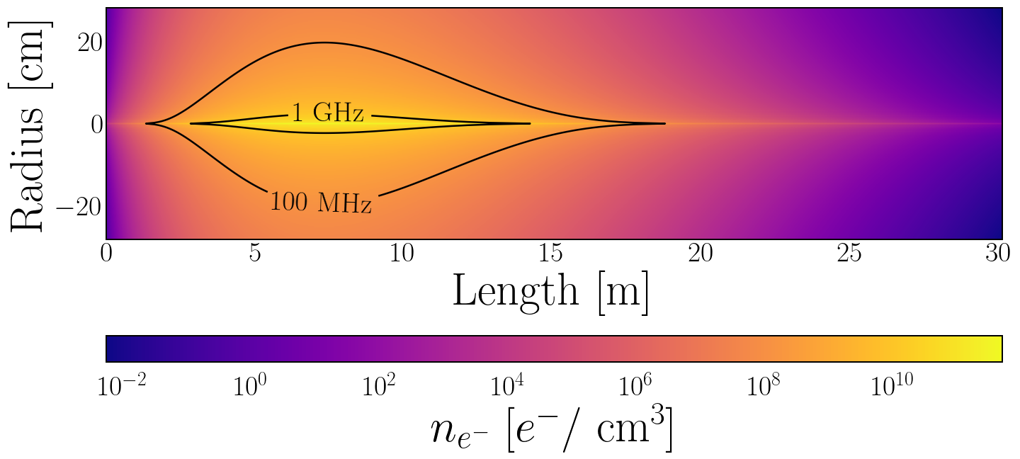
Figure 2: The cascade density profile $n_{e}$ of a $10^{7}$ GeV primary. The density and plasma frequency $\nu_{p}$ scale with the energy of the cascade’s primary, $E_{p}$. Curves of constant plasma frequency (and density) have been added for reference.

IV Scattering off of the cascade

In the tens of MHz to GHz regime, the transmitted wavelength, $\lambda_{T}$, becomes the smallest scale under consideration, $O(10\text{~{}cm}-10\text{~{}m})$. Therefore, we cannot approximate the ionization plasma left in the wake of a high-energy particle cascade as a point-like object, but have to consider its structure.

A more general description is found in describing the cascade as a collection of $M$ segments, each consisting of $N_{i}$, $i=1,..,M$ coherently scattering charges. The segment volumes need to be small enough to preserve coherence under $\lambda_{T}$. As such, in this work we use volumes of size $O(0.1\;\mathrm{cm}^{3})$. The volume size of an individual segment is, however, a free parameter of the model, and we have confirmed that the simulation results presented here converge under decreasing segment volumes (see Appendix B).

In determining the observed field amplitude at our receiver from the full cascade, we now have to account for interference between the segments. Segmenting our cascade into $M$ coherent scattering volumes and considering the individual phases of the scattered field at the receiver allows obtaining the power at the receiver,

$$P_{R,cascade}\propto|\vec{E}_{R,cascade}(R,t)|^{2}=$$

$$|\sum_{i=1}^{M}{E}_{R,i}(R_{i},t)*e^{i(kR_{i}-\omega t+\psi)}|^{2}.$$ (21)

The phase per segment $\phi_{i}=kR_{i}-\omega t+\psi$ is composed of three terms:

• $kR_{i}=k(R_{T,i}+R_{R,i})$ captures the phase shift over the propagation of the wave from the transmitter scattered to the receiver.

• $\omega t$ captures the phase shift at the receiver, considering the time of emission.

• $\psi$ is the unique relative phase per element. Under the damped-driven oscillator model, there is a frequency dependent phase difference between the driving force and the movement of the oscillator,

  $$\psi=\arctan\left(\frac{\omega_{c}\omega}{\omega_{0}^{2}-\omega^{2}}\right)=\arctan\left(-\frac{\omega_{c}}{\omega}\right).$$ (22)

  In the over-damped limit under consideration ($w_{c}\gg w$), this phase is constant and equal to $\psi\simeq-\pi/2$.

Three additions have to be made to our model when considering scattering off of a realistic cascade.

First is the inclusion of the lifetime of the plasma under consideration. Including lifetime effects, the total number of particles inside a scattering segment becomes time dependent and is written as,

$$N_{i}(t,t_{0})=N_{0,i}\cdot e^{-\frac{t-t_{0}}{\tau}}\Theta(t-t_{0}),$$ (23)

with $t_{0}$, the time at which the segment is created, and $\Theta(x)$ denoting the Heaviside step function.

Second, we have to take into account that the incoming wave is not only attenuated by the medium, but that part of its power is scattered away by other segments along the line of sight between the transmitter and the segment under consideration as outlined in Section II. To account for this effect, we have to include the transparency factor, ${\cal T}$, defined in Eq. 16. The transparency factor will be included into the scattering cross-section for a single cascade segment. Therefore, the single segment scattering cross-section does not stand by itself, but rather considers previous segments along the line of sight to the transmitter. Incorporating both effects, the radar scattering cross-section for a single scattering segment is given by,

$$\sigma_{RCS,i}(t,t_{0})=\sigma_{Th}N_{e,i}^{2}(\omega^{2}W)^{2}\cdot G_{Hz}\cdot{\cal T}\cdot e^{-\frac{2(t-t_{0})}{\tau}}\Theta(t-t_{0}).$$ (24)

The third and final effect to include is the attenuation of the incoming wave by the medium in which it propagates before reaching the plasma. The attenuation length is a free parameter in our model and attenuates the final field by a factor, $E_{R,i}=E_{R,i}^{no\;att}e^{-(R_{T}+R_{R})/L_{att}}$. In the following, we fix the attenuation length to $L_{att}=1.45$ km [3]. Given that the attenuation length varies with location [3, 4], a specific attenuation length or parameterization is left to site-specific studies. Implementing this into Eq. 7, now allows us to obtain the amplitude of the field from a single cascade scattering segment at the receiver as,

$$|E_{R,i}|=\frac{\sqrt{2Z_{ice}P_{T}G_{T}}}{4\pi R_{T}R_{R}}\sqrt{\sigma_{RCS,i}}e^{-(R_{T}+R_{R})/L_{att}}.$$ (25)

IV.1 Geometry

Given the different scales in which the relevant physics of the scatter occur, different effects are evaluated in different frames of reference. The three relevant frames considered in this work are shown in Fig. 3(a) and discussed in detail in Appendix A.1. The first frame is the bi-static scattering frame $\{\vec{e_{x}},\vec{e_{y}},\vec{e_{z}}\}$, defined by the transmitter and receiver locations. The cascade frame defined by $\{\vec{e_{L}},\vec{e_{R}},\vec{e_{n}}\}$ and the plane of incidence frame defined by $\{\vec{e_{U}},\vec{e_{V}},\vec{e_{W}}\}$, are both needed to compute the cascade response and the transparency factor ${\cal T}$.

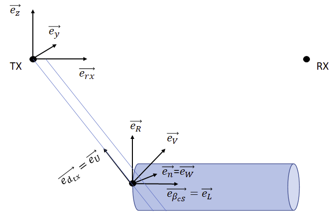
(a) The reference frames considered for this work. For illustration purposes, the cascade is directed along the $\vec{e}_{RX}$ axis in the $(\vec{e}_{rx},\vec{e}_{z})$ plane. In this case, the vectors $\vec{e}_{y}$, and $\vec{e}_{n}=\vec{e}_{W}$ are directed into the paper and all other vectors lie in the transmitter, receiver, cascade plane.

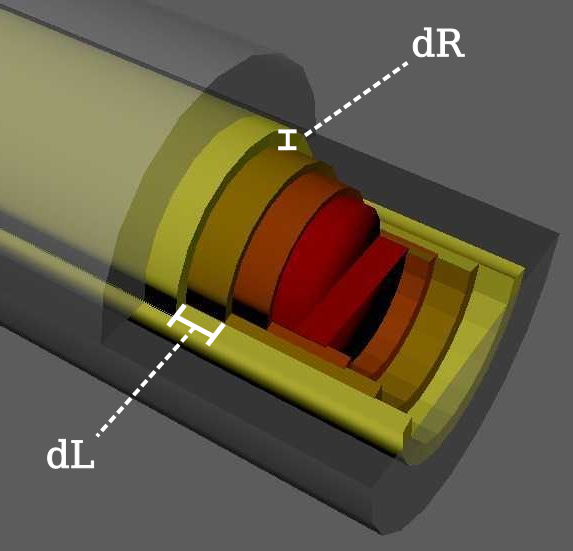
(b) Illustration of the cascade segmentation into semicircular rings.

Figure 3: The segmentation of the cascade. The cascade is sliced along the line of sight vector $\vec{e}_{U}$ (top). The segmentation is done using semicircular rings of width $\Delta L=1$ cm, radially subdivided with a thickness of $\Delta r=1$ mm (bottom).

The cascade segmentation is done by considering semi-circular ring segments in the cascade frame defined along the line of sight direction $\vec{e_{U}}$, as illustrated in Fig. 3(b). Each ring segment has a constant radial thickness of $\Delta r=1$ mm and width along the cascade axis of $\Delta L=1$ cm. Both dimensions are chosen such that the particle density is, to very good approximation, constant within the half-circular ring segment, which is small enough to fulfill the coherence requirement for an individual segment. These parameters have been checked for convergence (see Appendix B), and they remain independent of the results presented here.

A further approximation is subsequently made by positioning all half-circular ring segments along a ray path into a single coherent scattering center located at the intersection of the incoming ray with the cascade axis, defined by the center of the innermost ring. Placing the segments at the cascade axis along the line of sight from the transmitter has the advantage that ${\cal T}$ is directly obtained and numerically efficient to implement, but does introduce a small error in our calculation due to the slightly incorrect placement of the segments. However, given that most of the particles are located (very) close to the cascade axis, the induced error is small. For example, a ray crossing a cascade segment at $r=2$ cm from the cascade axis under 80 degrees incidence is placed incorrectly by $O(\mathrm{cm})$.

V Results

In this section, we discuss relativistic propagation effects as well as the effect of the finite lifetime of the cascade. Furthermore, we apply our model to the SLAC T-576 experiment and confirm that the observed scatter is consistent with our model prediction.

V.1 Lifetime

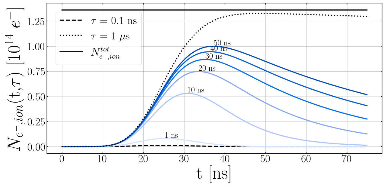
(a) The free ionization electron number as function of time for a $E_{p}=10^{7}$ GeV cascade. The straight, top line is the total amount of electrons ionized by the cascade, and represents the theoretical maximum of electrons that can be scattered off.

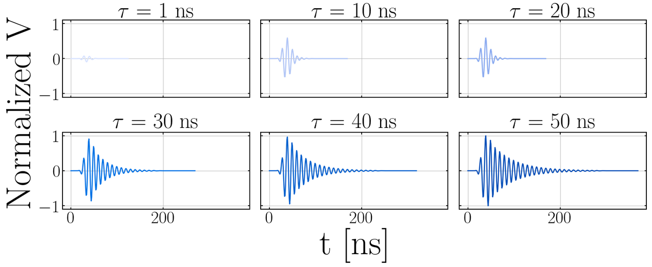
(b) Illustration of the effect of different free ionization electron lifetimes on the expected pulse shape. The pulse amplitude is normalized to its peak found for $\tau=50$ ns.

Figure 4: The effect of the ionization electron plasma lifetime on the total number of particles available for scattering at any instant in time (4(a)), and the observed (normalized) pulse shape at the detector (4(b)).

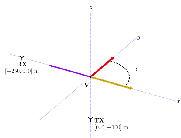
(a) The cascade interaction point is set at $V(0,0,0)$. The cascade direction is indicated by the colored arrows. The cascade is rotated in the $xy$-plane through the angle $\delta$, defined by $\delta=0^{\circ}$ (yellow) for cascade propagation along the x-axis and $\delta=90^{\circ}$ (red) along the y-axis and $\delta=180^{\circ}$ (purple) along the $-\hat{x}$-axis. The receiver is located in the $xy$-plane at $Rx(-250,0,0)$ m. The transmitter is located at $z=-100$ m, directly below the cascade vertex at $Tx(0,0,-100)$ m.

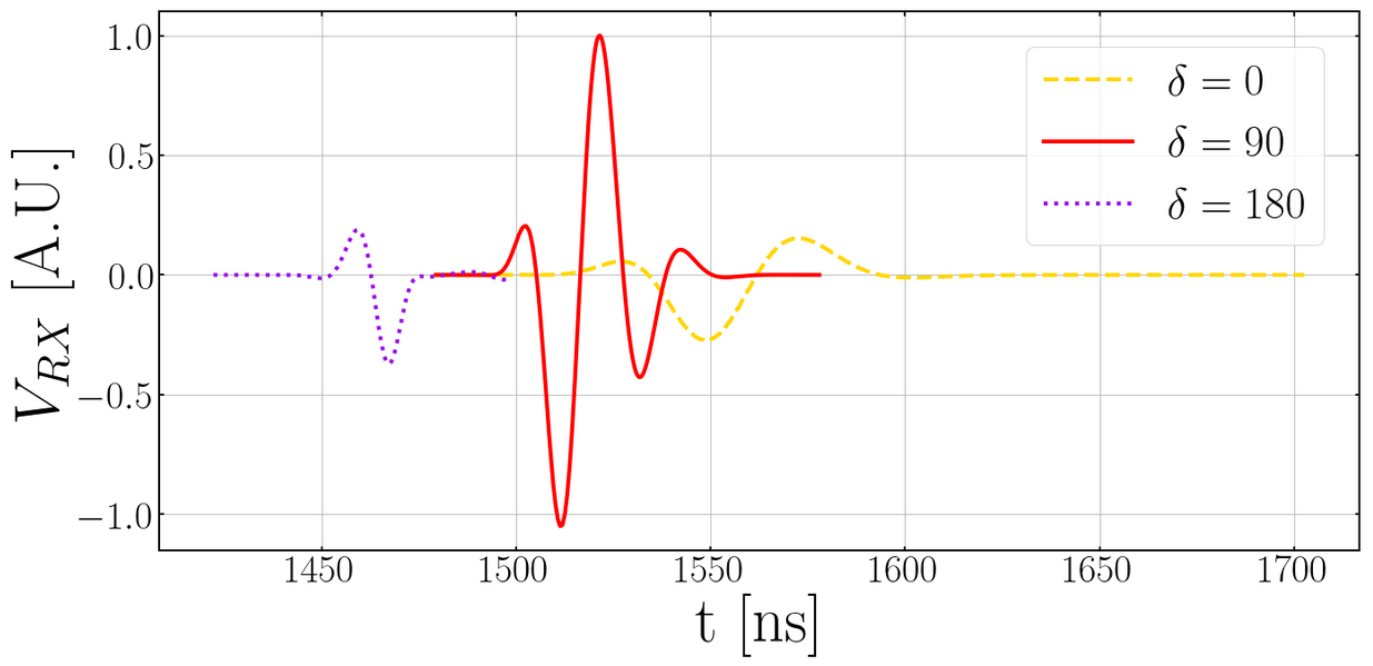
(b) MARES waveforms considering three events in the $xy$-plane at $\delta=0^{\circ}$ (yellow striped line) $\delta=90^{\circ}$ (full red line) and $\delta=180^{\circ}$ (purple dotted line). At $t=0$ the cascade is initiated. The amplitude has been normalized to the highest voltage.

Figure 5:

As introduced in Section III, and outlined in Appendix C, the plasma lifetime depends on the medium temperature and purity and ranges from $\tau\sim O(1-50)$ ns. Here we describe its effect on the scatter. If a cascade of energy $E_{p}$ starts at a $t=0$, the amount of free electrons at any given instant can be described as the convolution of Eqs. 18 and 23:

$$N_{e^{-},ion}(E_{p},t,\tau)=N(E_{p},t\cdot c\cdot\rho_{ice})\circledast e^{-\frac{t}{\tau}}\Theta(t),$$ (26)

where we make use of $c$ (the speed of the cascade front) and the density of the medium $\rho_{ice}$ to find the column density. This is shown in Fig. 4(a), where we observe that $\tau$ shapes the peak number of electrons available for scattering ($\{N_{ion}(t,\tau)\}_{max}$) and the moment in time when it happens, both important effects for the radar scatter signal.

The effect on the plasma lifetime for a typical signal is shown in Fig. 4(b). It is seen that for short lifetimes, below approximately 30 ns, the pulse amplitude increases. For longer lifetimes, the amplitude is constant and maximal, as effectively the entire ionization trail is alive at a certain moment in time. Hence, for lifetimes longer than approximately 30 ns, the amplitude is no longer increasing, but the pulse duration is, and a clear exponential decay with its duration determined by the lifetime becomes apparent.

V.2 Realistic cascade simulations

The limited plasma lifetime and its relativistic propagation cause the scattering from different segments to interfere, and geometry-dependent signal features appear. This is investigated by considering different geometries for which relativistic propagation effects become apparent. To outline the effects of the relativistic propagation of the cascade, we show the simulated electric fields for three different radar scatter events with different geometries presented in Fig. 5.

The geometry under consideration is shown in Fig. 5(a), where we fix the interaction vertex to $(x,y,z)=(0,0,0)$ m, the receiver is located at $(x,y,z)=(-250,0,0)$ m and the transmitter is fixed 100 m below the interaction vertex at $(x,y,z)=(0,0,-100)$ m.

It should be noted that the described signal features strongly depend on the transmitter location relative to the cascade. As such, the features described below provide intuition on the process, but are not general given that we fix our transmitter. The cascade direction is restricted to the $xy$-plane, varying the angle $\delta$, where for $\delta=0^{\circ}$ the cascade is moving away from the receiver in the $+\hat{x}$ direction, rotating clockwise to $+\hat{y}$, the direction defined by $\delta=90^{\circ}$. The cascade direction is indicated by the purple, red and yellow arrows. The same color scheme is used in Fig. 5(b), to indicate the corresponding waveforms for these geometries.

Fig. 5(b) shows the raw electric field observed for a transmit frequency of 50 MHz, considering different cascade directions in the $xy$-plane. Here, relativistic effects become apparent. The pulse is most compressed containing higher frequencies relative to the transmit frequency when the cascade is moving toward the receiver ($\delta=180^{\circ}$, purple dotted line), and stretched, containing lower frequencies, when it is moving away from the receiver ($\delta=0^{\circ}$, yellow striped line). The higher amplitude pulse is seen at ($\delta=90^{\circ}$, red full line).

The overall more complicated three-body (transmitter-cascade-receiver) geometry demands for a more elaborate investigation to obtain a detailed explanation for the full phase-space, and will be discussed in a forthcoming paper.

V.3 The T-576 experiment

To date, the T-576 experiment at SLAC provides the only positive observation of a radar scatter from a high-energy particle cascade [21]. The target material in this case was not ice, but high density Polyethylene (HDPE), where it is noted that HDPE has very similar properties to ice. This provides us with a benchmark to test our model, and allows providing an independent verification of the obtained experimental results. In the following, we use the parameters published in [20, 21], summarized in Table 1. We deviate from our nominal value for the lifetime ($\tau_{nominal}=10$ ns), and use the value that was estimated in [21], based on the T576 observation, $\tau=3$ ns. Given the strong signal dependence on lifetime discussed in Fig. 4(b), we estimate its error at the ns level. The free charge collision frequency $\nu_{c}=100$ THz, as well as the mean electron ionization energy $E_{ion}=20$ eV are kept at their nominal values.

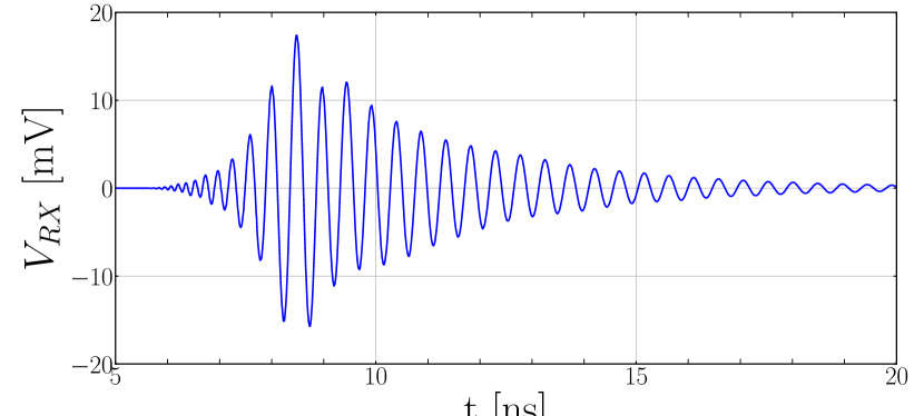
Figure 6: The predicted MARES signal of the T-576 experiment [21]

Parameters	Signal error estimate
Experimental configuration
$E_{p}=10~{}\mathrm{GeV}/\mathrm{e}^{-}$
$N_{p}=10^{9}~{}\mathrm{e}^{-}$
$\vec{x}_{t}=(-3.8,0,-0.3)~{}\mathrm{m}$
$\vec{x}_{r}=(-3.877,0,0.3)~{}\mathrm{m}$
$\vec{x}_{c}=(0,0,0)~{}\mathrm{m}$
$\lambda_{t}=2.1~{}\mathrm{GHz}$	$\sim 7$ dB (See Table 1 of  [21])
$P_{t}=50~{}\mathrm{W}$
$G_{t}=12~{}\mathrm{dB}$
$G_{r}=18~{}\mathrm{dB}$
$n=1.51$
MARES parameters	Signal error estimate
$E_{ion}=(20\pm 2)~{}\mathrm{eV}/\mathrm{e}^{-}$	$O(10\%)$
$\nu_{c}=(100\pm 50)~{}\mathrm{THz}$	$O(100\%)$
$\tau=(3\pm 1)$ ns	$O(33\%)$

Table 1: T576 parameters used as input for the MARES simulation, including error estimates. Error estimates on these parameters are taken from [21] if provided and elaborated upon in the text.

We performed a full MARES simulation using the framework outlined above, for which the result is shown in Fig. 6. As we provide an estimate that matches reality well, it is important to note the errors on the different parameters available for the simulation. As such, an estimate on these errors is also given in Table 1. It follows that our estimate should be interpreted at the order of magnitude level. To conclude, for the given geometry, the observed field amplitude is at the same order of magnitude compared to the amplitude found in Fig. 3 of [21].

VI Conclusions

We developed the MARES model to describe the radar echo from the ionization plasma left in the wake of a high-energy particle cascade developing in a dense medium like ice. The formalism is deterministic and allows for a computation of the scattering process, with a single simulation taking $O(\mathrm{s})$.

As a first application, we find good agreement with the radar echo signal observed at the SLAC T-576 experiment. Furthermore, we studied the effect of the free ionization charge lifetime on the expected radar signal and introduce a radar scatter example that highlights the relationship between the geometry of the scatter and the signal features. Both examples show how a deterministic model like MARES can be used to quantify these observables.

The MARES code is currently available within the RET collaboration, and will be made public in the near future.

Appendix A Frames of reference

A.1 The bi-static scattering frame

First, we define the bi-static scattering frame by placing the (0,0,0) origin at the transmitter (TX), the $\vec{e}_{rx}$ unit vector points from TX to the receiver (RX), and $\vec{e}_{z}$ is the vertical. We now define:

$$\vec{e}_{y}=\vec{e}_{z}\times\vec{e}_{rx}\ ;\ \vec{e}_{x}=\vec{e}_{y}\times\vec{e}_{z},$$ (27)

such that, $\{\vec{e}_{x},\vec{e}_{y},\vec{e}_{z}\}$ defines a right-handed orthogonal basis. In this frame, the cascade is defined by the interaction vertex $\vec{V}_{CS}$, and the cascade direction $\vec{\beta}_{CS}$. This frame allows to directly evaluate the bi-static radar scattering equation for our segments.

A.2 The cascade frame

The cascade frame is defined by the cascade direction $\vec{e}_{\beta_{CS}}$ and the direction vector pointing from the cascade to the transmitter, $\vec{d_{tx}}=\vec{V}_{CS}-\vec{0}$, with unit vector $\vec{e}_{d_{tx}}$. The cascade frame is defined by $\{\vec{e}_{L},\vec{e}_{R},\vec{e}_{n}\}$. Here,

$$\vec{e}_{L}=\vec{e}_{\beta_{CS}}\ ;\ \vec{e}_{n}=\vec{e}_{L}\times\vec{e}_{d_{tx}}\ ;\ \vec{e}_{R}=\vec{e}_{n}\times\vec{e}_{L}.$$ (28)

This frame allows for a universal cascade parameterization along its longitudinal direction $\vec{e}_{L}$, and radial direction $\vec{e}_{R}$.

A.3 The plane of incidence frame

The plane of incidence frame is defined as $\{\vec{e}_{U},\vec{e}_{V},\vec{e}_{W}\}$ and is constructed similarly as the cascade frame,

$$\vec{e}_{U}=\vec{e}_{d_{tx}}\ ;\ \vec{e}_{V}=\vec{e}_{n}\times\vec{e}_{d_{tx}}\ ;\ \vec{e}_{W}=\vec{e_{n}}.$$ (29)

The line of sight from the transmitter to the cascade, and thus the direction of propagation of the transmitted radio wave is defined by $\vec{e}_{U}$. The polarization of the emitted radio wave is now naturally found in the $\{\vec{e}_{V},\vec{e}_{W}\}$ plane.

Note that this frame is orthogonal only in the plane wave approximation, which is valid under the condition that the effective length of the cascade in ice, $L$, is small compared to the distance to the antennas $R_{T},R_{R}$, such that the incidence angle along the cascade is constant to good approximation.

Appendix B Convergence

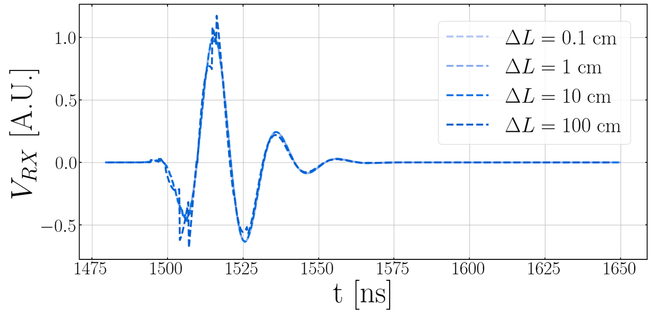
(a) Convergence of the step size parameter $\Delta L$, fixing $\Delta r$ to its nominal value, $\Delta r=1$ mm.

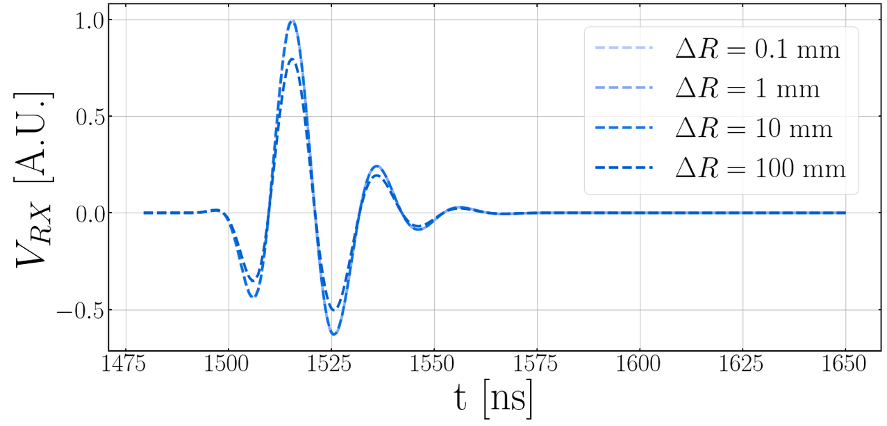
(b) Convergence of the step size parameter $\Delta r$, fixing $\Delta L$ to its nominal value, $\Delta L=1$ cm.

Figure 7: Convergence over the segmentation step size parameters $\Delta L$ and $\Delta r$ considering the geometry outlined in Fig. 5(a), using $\delta=90^{\circ}$, and $\theta=90^{\circ}$. The pulse peak amplitude is normalized to the amplitude found using the nominal values $\Delta L=1$ cm and $\Delta r=1$ mm.

To check for convergence of the MARES model over its segmentation steps, $\Delta L$, and $\Delta r$, we consider the geometry outlined in Fig. 5(a), using $\delta=90^{\circ}$, and $\theta=90^{\circ}$, for which the projected cascade size towards the observer is maximized. In Fig. 7(a), we fix $\Delta r$ to its nominal value $\Delta r=1$ mm, and vary $\Delta L$, where in Fig. 7(b) we fix $\Delta L$ to its nominal value $\Delta L=1$ cm, and vary $\Delta r$. It follows that the results converge for step sizes roughly a factor of 10 above the nominal values used for this work. However, given that this only considers a single geometry, we recommend using the nominal step size when running the simulation.

Appendix C Free electron lifetime

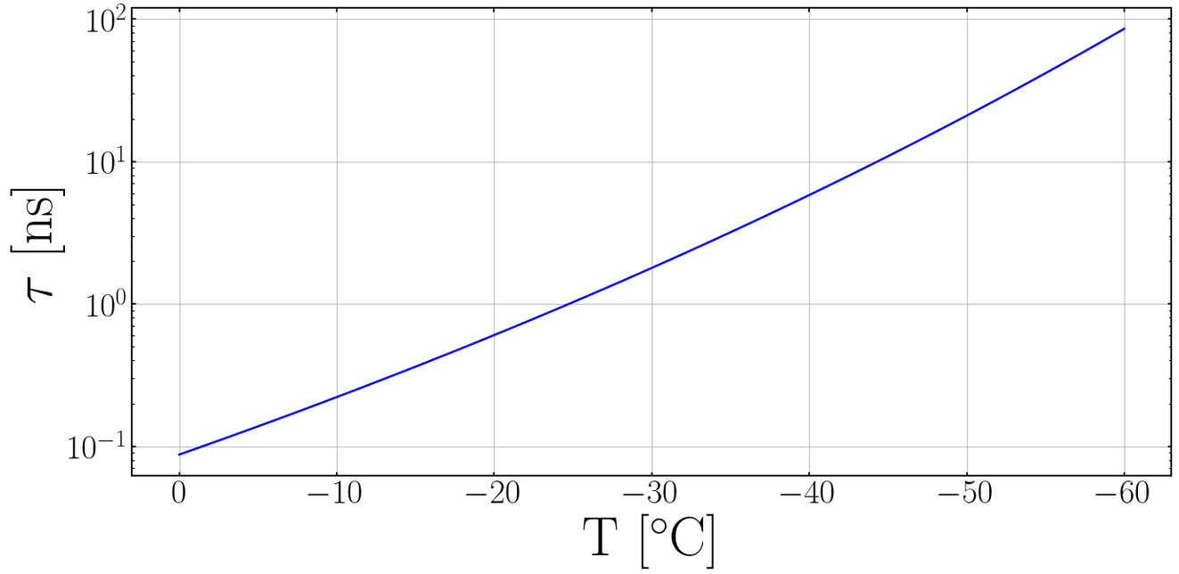
Figure 8: The free electron lifetime as function of temperature.

The total number of free ionization electrons available for scattering is well described through a standard decay $N(t,\tau)=N(t=0,\tau)e^{-t/\tau}$, assuming the ionization occurs at the time $t=0$. Here, $\tau$ denotes the free electron lifetime.

As such, we are interested in obtaining an accurate value, or range of values, for the free electron lifetime, $\tau$, for ice. Over the last few decades, several measurements have been made that allow to determine $\tau$ for ice. We are interested in the temperature range of ice typically found in polar regions, T=[$-60^{\circ}~{}$C, $0^{\circ}$ C] [36, 37]. Therefore, following a recent overview work [38], we base ourselves on results obtained in 1952 by Auty and Cole [39], and related measurements by De Haas et al., in 1983 [29].

Auty and Cole took measurements of the dielectric constant of ice to obtain the dielectric relaxation time $\tau_{c}$ (not to be confused with the free electron lifetime),

$$\tau_{c}=Ae^{\frac{B}{k_{B}T}}$$ (30)

with A = $5.3\cdot 10^{-16}$ s, $B=0.575$ eV, and $k_{B}=8.617\cdot 10^{-5}\;\mathrm{eV\;K^{-1}}$, where the latter is Boltzmann’s constant.

These results were subsequently used by De Haas et al., who performed a series of measurements to obtain the free electron lifetime in ice as function of temperature. This was done by directing X-ray or 3 MeV electron bunches into a block of ice, after which the ice conductivity was obtained as a function of time [29].

In Fig. 3 of [29], the electron trapping rate in ice, $f_{r}=1/\tau\mathrm{[s^{-1}]}$, is presented as a function of reciprocal temperature $10^{3}/T\;\mathrm{[K^{-1}]}$ and fitted using the Arrhenius equation to obtain:

$$\tau=\tau_{c}/C=(A/C)e^{\frac{B}{k_{B}T}}$$ (31)

with $C$ a scale factor reported in the caption of Fig. 3 of  [29], equal to $C=1/(2.5\cdot 10^{5})$, and $\tau_{C}$ is taken from the Auty and Cole measurements.

This allows us to calculate the free electron lifetime over our temperature range of interest, $T=[-60^{\circ}$ C, $0^{\circ}$ C], as shown in Fig. 8. It follows, the lifetime ranges from roughly 0.1 ns at $0^{\circ}$ C up to $100$ ns at $-60^{\circ}$ C.

References

- [1] IceCube collaboration, Evidence for high-energy extraterrestrial neutrinos at the icecube detector, Science 342 (2013) 1242856.
- [2] IceCube collaboration, Improved Characterization of the Astrophysical Muon–neutrino Flux with 9.5 Years of IceCube Data, Astrophys. J. 928 (2022) 50 [2111.10299].
- [3] D. Besson et al., In situ radioglaciological measurements near taylor dome, antarctica and implications for ultra-high energy (uhe) neutrino astronomy, Astropart. Phys. 29 (2008) 130.
- [4] J.A. Aguilar et al., In situ, broadband measurement of the radio frequency attenuation length at summit station, greenland, J Glaciol 68 (2022) 1234–1242.
- [5] F.G. Schröder, Radio detection of cosmic-ray air showers and high-energy neutrinos, Prog. Part. Nucl. Phys. 93 (2017) 1.
- [6] G.A. Askaryan, Excess negative charge of an electron-photon shower and its coherent radio emission, Sov. Phys. JETP 14 (1962) 441.
- [7] K. Bechtol et al., SLAC T-510 experiment for radio emission from particle showers: Detailed simulation study and interpretation, Phys. Rev. D 105 (2022) 063025.
- [8] Codalema collaboration, Evidence for the charge-excess contribution in air shower radio emission observed by the codalema experiment, Astropart. Phys. 69 (2015) 50.
- [9] Pierre Auger collaboration, Probing the radio emission from air showers with polarization measurements, Phys. Rev. D 89 (2014) 052002 [1402.3677].
- [10] P.M.S. Blackett and A.C.B. Lovell, Radio echoes and cosmic ray showers, Proc. R. Soc. Lond. A 177 (1941) 183–186.
- [11] A.C.B. Lovell, Reminiscences and discoveries: The Blackett-Eckersley-Lovell correspondence of World War II and the origin of Jodrell Bank, Notes Rec. R. Soc. Lond. 47 (1) (1993) 119.
- [12] T. Matano et al., Tokyo large air shower project, Can J Phys 46 (1968) S255.
- [13] P.W. Gorham, On the possibility of radar echo detection of ultra-high energy cosmic ray- and neutrino-induced extensive air showers, Astropart. Phys. 15 (2001) 177.
- [14] J. Stasielak et al., Radar reflection off extensive air showers, EPJ Web of Conferences 53 (2013) 08013.
- [15] A.D. Filonenko, Coherent Scattering of Monochromatic RF Radiation by Ionization Electrons of an Extensive Air Shower., J. Exp. Theor. Phys. 117 (2013) 641–648.
- [16] Tara collaboration, First upper limits on the radar cross section of cosmic-ray induced extensive air showers, Astropart. Phys. 87 (2017) 1.
- [17] M. Chiba et al., Radar for detection of ultra-high-energy neutrinos reacting in a rock salt dome, Nucl. Instrum. Meth. A” 662 (2012) S222.
- [18] K.D. de Vries, K. Hanson and T. Meures, On the feasibility of radar detection of high-energy neutrino-induced showers in ice, Astropart. Phys. 60 (2015) 25.
- [19] K.D. de Vries, K. Hanson, T. Meures and A. O’Murchadha, On the feasibility of radar detection of high-energy cosmic neutrinos, PoS ICRC2015 (2015) 1168.
- [20] S. Prohira et al., Suggestion of coherent radio reflections from an electron-beam induced particle cascade, Phys. Rev. D 100 (2019) 072003.
- [21] S. Prohira et al., Observation of radar echoes from high-energy particle cascades, Phys. Rev. Lett. 124 (2020) 091101.
- [22] S. De Kockere et al., Simulation of in-ice cosmic ray air shower induced particle cascades, Phys. Rev. D 106 (2022) 043023.
- [23] Radar Echo Telescope collaboration, The radar echo telescope for cosmic rays: Pathfinder experiment for a next-generation neutrino observatory, Phys. Rev. D 104 (2021) 102006.
- [24] Radar Echo Telescope collaboration, The Radar Echo Telescope for Neutrinos, PoS ICRC2021 (2021) 1195.
- [25] H. Takai, I. Myers and J. Belz, Forward Scattering Radar for Ultra High Energy Cosmic Rays, in 32nd International Cosmic Ray Conference, vol. 3, p. 344, 2011.
- [26] S. Prohira and D. Besson, Particle-level model for radar based detection of high-energy neutrino cascades, Nucl. Instrum. Methods. Phys. Res. A 922 (2019) 161.
- [27] S.Agostinelli et al.Nucl. Instrum. Methods Phys. Res. A 506 (2003) 250.
- [28] C.A. Balanis, Antenna theory: analysis and design, Wiley-Interscience, 3 ed. (2005).
- [29] M.P. De Haas et al., Nanosecond time-resolved conductivity studies of pulse-ionized ice. 1. The mobility and trapping of conduction-band electrons in water and deuterium oxide ice, J. Phys. Chem. 87 (1983) 4089.
- [30] J.R. Taylor, Classical Mechanics, University Science Books, 1st ed. (2005).
- [31] J.D. Jackson, Classical Electrodynamics, Wiley, 3rd ed. (1999).
- [32] J.G. Wilson and K. Greisen, Progress in Cosmic Ray Physics, vol. 3, p. 17, North Holland Amsterdam (1956).
- [33] J.A.J. Matthews et al., A parameterization of cosmic ray shower profiles based on shower width, J. Phys. G: Nucl. Part. Phys. 37 (2010) 025202.
- [34] K. Kamata and J. Nishimura, The Lateral and the Angular Structure Functions of Electron Showers, Prog. theor. phys., Suppl. 6 (1958) 93.
- [35] N. Tîmneanu et al., Auger electron cascades in water and ice, Chemical Physics 299 (2004) 277.
- [36] P.P. Buford et al., Temperature profile for glacial ice at the south pole: Implications for life in a nearby subglacial lake, PNAS USA 99 (2002) 7844.
- [37] J.A. MacGregor et al., Radar attenuation and temperature within the greenland ice sheet, J. Geophys. Res. Earth. Surf. 120 (2015) 983.
- [38] A.A. Khamzin et al., Theoretical description of dielectric relaxation of ice with low concentration impurities, Chem. Phys. 541 (2021) 111040.
- [39] R.P. Auty and R.H. Cole, Dielectric Properties of Ice and Solid D2O, J. Chem. Phys. 20 (1952) 1309.