A Divergence-Free and $H(div)$-Conforming
Embedded-Hybridized DG Method for
the Incompressible Resistive MHD equations

Abstract

We proposed a divergence-free and $H\left(div\right)$-conforming embedded-hybridized discontinuous Galerkin (E-HDG) method for solving stationary incompressible viso-resistive magnetohydrodynamic (MHD) equations. In particular, the E-HDG method is computationally far more advantageous over the hybridized discontinuous Galerkin (HDG) counterpart in general. The benefit is even significant in the three-dimensional/high-order/fine mesh scenario. On a simplicial mesh, our method with a specific choice of the approximation spaces is proved to be well-posed for the linear case. Additionally, the velocity and magnetic fields are divergence-free and $H\left(div\right)$-conforming for both linear and nonlinear cases. Moreover, the results of well-posedness analysis, divergence-free property, and $H\left(div\right)$-conformity can be directly applied to the HDG version of the proposed approach. The HDG or E-HDG method for the linearized MHD equations can be incorporated into the fixed point Picard iteration to solve the nonlinear MHD equations in an iterative manner. We examine the accuracy and convergence of our E-HDG method for both linear and nonlinear cases through various numerical experiments including two- and three-dimensional problems with smooth and singular solutions. For smooth problems, the results indicate that convergence rates in the $L^{2}$ norm for the velocity and magnetic fields are optimal in the regime of low Reynolds number and magnetic Reynolds number. Furthermore, the divergence error is machine zero for both smooth and singular problems. Finally, we numerically demonstrated that our proposed method is pressure-robust.

65N30, 76W05

1 Introduction

Magnetohydrodynamics (MHD) is a field within continuum mechanics that investigates the behavior of electrically conducting fluids in the presence of magnetic fields [31]. This coupled phenomenon holds significant importance across various sectors, including astrophysics [46, 47], planetary magnetism [20, 61], nuclear engineering [76, 39, 87], and the metallurgical industry [1, 30].

We consider a standard form of the stationary incompressible MHD equations as derived in [5]; see also [42, 43, 49]. Specifically, we omit effects related to high-frequency phenomena and convection current, focusing on a medium that is non-polarizable, non-magnetizable, and homogeneous

(1a) $$-\frac{1}{\textup{Re}}\Delta\boldsymbol{u}+\nabla p+(\boldsymbol{u}\cdot\nabla)\boldsymbol{u}+\kappa\boldsymbol{b}\times(\nabla\times\boldsymbol{b}) =\boldsymbol{g},$$

(1b) $$\nabla\cdot\boldsymbol{u} =0,$$

(1c) $$\frac{\kappa}{\textup{Rm}}\nabla\times(\nabla\times\boldsymbol{b})+\nabla r-\kappa\nabla\times(\boldsymbol{u}\times\boldsymbol{{d}}) =\boldsymbol{f},$$

(1d) $$\nabla\cdot\boldsymbol{b} =0,$$

where $\boldsymbol{u}$ is the velocity of the fluid (plasma or liquid metal), $\boldsymbol{b}$ the magnetic field, $p$ the fluid pressure, and $r$ a Lagrange multiplier that is associated with divergence constraint (1d) on $\boldsymbol{b}$. The system (1) is characterized by three dimensionless parameters: a fluid Reynolds number $\textup{Re}>0$, a magnetic Reynolds number $\textup{Rm}>0$, and a coupling parameter $\kappa=\textup{Ha}^{2}/(\textup{Re}\textup{Rm})$, with the Hartmann number $\textup{Ha}>0$. For a deeper exploration of these parameters and their usual values, we suggest referring to additional resources [5, 43, 31].

The major challenges in discretization of the MHD equations are: (i) The multi-physics feature. The occurrence of distinct physics could lead to disparate temporal (for the time-dependent MHD equations) and spatial scales. (ii) The nonlinearity. (iii) Incompressibility. The satisfaction of exact mass conservation stated in (1b) is closely tied to the concept of pressure-robust which is the statement about the lack of correlation between a priori error estimate for the velocity and the pressure error [73, 74, 57]. Significant solution error can be induced without global enforcement of the continuity equation in a pointwise manner [73, 74, 57]. By globality, we mean that the jump of the normal component of velocity has to vanish across the interior boundaries of elements on a given mesh. In addition to the large error in the solution, when utilizing a computed velocity field that doesn’t exactly maintain mass conservation as the advective velocity in a transport solver, spurious results could be introduced and could undermine the stability of the transport equation [83]. (iv) The solenoidal constraint for the magnetic field. The violation of this constraint will cause the wrong topologies of magnetic field lines, leading to plasma transport in an incorrect direction. Furthermore, nonphysical force proportional to the divergence error could be created, potentially inducing instability [19, 11, 89]. (v) The dual saddle-point structure of the velocity-pressure. The discretized system is subject to having a notorious conditional number owing to such a structure and thus is difficult to solve.

Many numerical schemes have been proposed to solve linear and nonlinear, time-dependent, and -independent MHD systems. Regarding spatial discretization, hybridized discontinuous Galerkin (HDG) methods have demonstrated remarkable success [67, 23, 80, 62, 45, 77]. The HDG methods were first introduced under the context of symmetric elliptic problems [25] to overcome the common criticism had by discontinuous Galerkin (DG) methods which require significantly more globally coupled unknowns than continuous Galerkin methods due to the duplication of degrees of freedoms (DOFs) on element boundaries [24]. The HDG methods reduce the computational cost of DG methods by introducing variables uniquely defined on the intersections of element boundaries and removing local (element-wise) DOFs through static condensation which was initially used in mixed finite element methods (i.e.,[16]). Consequently, the HDG methods are more efficient while retaining the attractive features of DG methods such as being highly suitable for solving convection-dominated problems in complex geometries, delivering high-order accuracy in approximations, and accommodating $h$/$p$ refinement [52]. The computational cost of HDG methods can be further lowered by making facet variables introduced in HDG methods continuous across the skeleton of the mesh. These methods are referred to as the embedded discontinuous Galerkin (EDG) methods and were first proposed for solving elliptic problems in [51]. Later, an EDG method was developed for incompressible flow in [63, 64] where it showed that the method inherited many of the desirable features of DG methods but only required the same amount of DOFs as the continuous Galerkin method on a given mesh. Unfortunately, the conservative property can be compromised by the employment of the EDG method [64]. In particular, the velocity field is not globally pointwise divergence-free, and the mass is only weakly conserved in the local sense. To strike a balance between HDG and EDG methods, an embedded-hybridized discontinuous Galerkin (E-HDG) method was first developed in [84] for Stokes equations. The method is proved to be globally pointwise-divergence-free and automatically divergence-conforming. Further, the number of global DOFs can be substantially reduced by using a continuous basis for facet velocity field while maintaining a facet pressure discontinuous over facets. The methodology was later adopted to space-time discretization to solve incompressible flow on moving domains [53, 54] and is proved to be exactly global mass conserving, locally momentum conserving, and energy-stable.

To address the issue of the divergence-free constraint on the velocity field, several approaches have been suggested within the framework of DG, HDG, or E-HDG methods. A way to achieve it is to use divergence-conforming elements in the approximation of velocity. It is discussed in [27, 48, 40] for DG methods. Alternatively, the constraint can be satisfied locally using solenoidal approximation space for DG methods [8, 58, 70, 92, 60] and globally for HDG methods [21]. On the other hand, divergence-conformity can be acquired with the help of facet variables and proper design of numerical flux for HDG [68, 69, 82, 65, 83, 78, 45] and E-HDG [84, 53, 54] methods. Another option to obtain globally divergence-free methods is to perform post-processing using special projection operators [14, 26, 90, 28, 29, 50, 66]. One can also apply pressure-correction methods that relies on Helmholtz decomposition to maintain the divergence-free constraint [18, 59].

We remark that the divergence-free constraint on the magnetic field given in (1d) can be implied by the initial condition in the context of time-dependent MHD equations on the continuous level and it is also known as the solenoidal involution property of the magnetic field. However, such a property can be destroyed by temporal and spatial discretization errors. There are numerous methods that have been proposed to satisfy the $\nabla\cdot{\boldsymbol{b}}=0$ constraint in MHD calculations and some of the ideas can be linked to the approaches developed to handle the $\nabla\cdot{\boldsymbol{u}}=0$ constraint in the context of solving incompressible flow. These methods include source term methods [79, 56], the projection method [19, 33] (similar to the projection-correction methods [18, 59]), the hyperbolic divergence cleaning methods [32, 60, 17, 23] (similar to artificial compressibility methods [12, 13]), the locally divergence-free methods [70, 92] (use locally solenoidal approximation space and is similar to [8, 58, 60]), the globally divergence-free methods [40] (use globally solenoidal approximation space), and the constrained transport (CT) methods [36, 11, 75, 89]. We would like to note that the works on DG methods [88, 72, 71] for solving the ideal MHD system can be interpreted as high-order CT-type methods. A similar idea is also extended to solve the incompressible MHD system as well [41]. In this work, we focus on the stationary incompressible MHD system stated in (1), and the divergence-free constraint on the magnetic field is solved together with the entire system augmented by the Lagrange multiplier $r$. The resulting formulation is amenable to obtaining divergence-conforming finite element methods through the hybridization of facet Lagrange multiplier variable [45]. Again, the globally divergence-free property of the magnetic field can also be achieved by post-processing [66, 80] within the scope of the DG/HDG methods.

In this paper, we devised a divergence-free and $H\left(div\right)$-conforming E-HDG meth-
-od for solving the stationary incompressible viso-resistive MHD equations given in (1). To that end, a divergence-conforming E-HDG method for the linearized MHD system is proposed. The conformity can be achieved, by following an idea similar to [84, 53], through hybridization via a facet pressure and a facet Lagrange multiplier field which is discontinuous between facets, as is a typical HDG method [45]. In this paper, we extended the work [67] and ensure divergence-free and $H\left(div\right)$-conforming properties. This is in contrast to the work [45] where the authors hybridized the other popular class of DG methods called interior penalty discontinuous Galerkin (IPDG) methods [34, 7, 91, 6, 8] to construct the divergence-free and divergence-conforming HDG method for the time-dependent incompressible viso-resistive MHD equations. To ensure stability, the penalty parameter in IPDG methods, as the one in typical Nitsche methods, needs to be set to be sufficiently large. Nonetheless, the information on how exactly large it should be is unavailable. On the other hand, our approach does not suffer from such difficulty and the criteria of the stabilization parameters are well-defined. Toward being embedded and hybridized, we use a continuous basis for facet velocity and facet magnetic field. With a few assumptions, our proposed scheme is proved to be well-posed as long as the stabilization parameters satisfy certain criteria. The resultant E-HDG discretization for the linearized model is then incorporated into the fixed point Picard iteration to construct a fully nonlinear solver. Moreover, divergence-free and $H\left(div\right)$-conforming properties still hold for the nonlinear case. Finally, we remark that divergence-free and $H\left(div\right)$-conforming HDG version of the proposed approach can be easily obtained by mild modification of the approximation space for facet variables. Further, all results we discussed in the context of our E-HDG method are still applied, including well-posedness, divergence-free property, and $H{div}$-conformity.

The paper is organized as follows. Section 2 outlines the notations. In Section 3 both the HDG and E-HDG formulation for the linearized incompressible viso-resistive MHD equations are proposed. In addition, the well-posedness of both formulations is proved. Further, we proved the divergence-free property and $H\left(div\right)$-conformity of both velocity (i.e., pointwise mass conservation) and magnetic (i.e., pointwise absence of magnetic monopoles) fields for linear and nonlinear cases. The implementation aspect is discussed in Section 4 where we also compared the computational costs required by HDG and E-HDG methods. Several numerical examples for linear and nonlinear incompressible viso-resistive MHD equations are presented to demonstrate the accuracy and convergence of our proposed methods in both two- and three-dimensional settings. Section 5 concludes the paper with future work.

2 Notations

In this section, we introduce common notations and conventions to be used in the rest of the paper. Let $\Omega\subset{\mathbb{R}}^{d}$, $d=2,3$, be a bounded domain such that it is simply connected and its boundary ${\partial\Omega}$ is a Lipschitz manifold with only one component. Suppose that we have a triangulation of $\Omega$ and partition $\Omega$ into a finite number of nonoverlapping $d$-dimensional simplices, i.e., triangle and tetrahedron for two and three dimensions, respectively. We assume that the triangulation is shape-regular, i.e., for all $d$-dimensional simplices in the triangulation, the ratio of the diameter of the simplex and the radius of an inscribed $d$-dimensional ball is uniformly bounded. We will use ${\Omega_{h}}$ and ${\mathcal{E}_{h}}$ to denote the sets of $d$- and ($d-1$)-dimensional simplices of the triangulation and call ${\mathcal{E}_{h}}$ the mesh skeleton of the triangulation. The boundary and interior mesh skeletons are defined by ${\mathcal{E}_{h}^{\partial}}:=\{e\in{\mathcal{E}_{h}}\,:\,e\subset\partial\Omega\}$ and ${\mathcal{E}_{h}^{o}}:={\mathcal{E}_{h}}\setminus{\mathcal{E}_{h}^{\partial}}$. We also define ${{\partial\Omega}_{h}}:=\left\{{\partial K}:K\in{\Omega_{h}}\right\}$. The mesh size of triangulations is $h:=\max_{K\in{\Omega_{h}}}\text{diam}(K)$.

We use $\left(\cdot,\cdot\right)_{D}$ (respectively $\left<\cdot,\cdot\right>_{D}$) to denote the $L^{2}$-inner product on $D$ if $D$ is a $d$- (respectively $(d-1)$-) dimensional domain. The standard notation $W^{s,p}(D)$, $s\geq 0$, $1\leq p\leq\infty$, is used for the Sobolev space on $D$ based on $L^{p}$-norm with differentiability $s$ (see, e.g., [37]) and $\left\|\cdot\right\|_{W^{s,p}(D)}$ denotes the associated norm. In particular, if $p=2$, we use $H^{s}(D):=W^{s,2}(D)$ and $\left\|\cdot\right\|_{s,D}$. $W^{s,p}({\Omega_{h}})$ denotes the space of functions whose restrictions on $K$ reside in $W^{s,p}(K)$ for each $K\in{\Omega_{h}}$ and its norm is $\left\|u\right\|_{W^{s,p}({\Omega_{h}})}^{p}:=\sum_{K\in{\Omega_{h}}}\left\|u|_{K}\right\|_{W^{s,p}(K)}^{p}$ if $1\leq p<\infty$ and $\left\|u\right\|_{W^{s,\infty}({\Omega_{h}})}:=\max_{K\in{\Omega_{h}}}\left\|u|_{K}\right\|_{W^{s,\infty}(K)}$. For simplicity, we use $\left(\cdot,\cdot\right)$, $\left<\cdot,\cdot\right>$, $\left\|\cdot\right\|_{s}$, $\left\|\cdot\right\|_{{{\partial\Omega}_{h}}}$, and $\left\|\cdot\right\|_{W^{s,\infty}}$ for $\left(\cdot,\cdot\right)_{\Omega}$, $\left<\cdot,\cdot\right>_{{{\partial\Omega}_{h}}}$, $\left\|\cdot\right\|_{s,\Omega}$, $\left\|\cdot\right\|_{0,{{\partial\Omega}_{h}}}$, and $\left\|\cdot\right\|_{W^{s,\infty}({\Omega_{h}})}$, respectively.

For vector- or matrix-valued functions these notations are naturally extended with a component-wise inner product. We define similar spaces (respectively inner products and norms) on a single element and a single skeleton face/edge by replacing ${\Omega_{h}}$ with $K$ and ${\mathcal{E}_{h}}$ with $e$. We define the gradient of a vector, the divergence of a matrix, and the outer product symbol $\otimes$ as:

$$\left(\nabla\boldsymbol{u}\right)_{ij}=\frac{\partial u_{i}}{\partial x_{j}},\quad\left(\nabla\cdot\boldsymbol{L}\right)_{i}=\nabla\cdot\boldsymbol{L}\left(i,:\right)=\sum_{j=1}^{d}\frac{\partial\boldsymbol{L}_{ij}}{\partial x_{j}},\quad\left(\boldsymbol{a}\otimes\boldsymbol{b}\right)_{ij}=a_{i}b_{j}=\left(\boldsymbol{a}\boldsymbol{b}^{T}\right)_{ij}.$$

The curl of a vector when $d=3$ takes its standard form, $\left(\nabla\times\boldsymbol{b}\right)_{i}=\sum_{j,k}\epsilon_{ijk}\frac{\partial\boldsymbol{b}_{k}}{\partial x_{j}}$, where $\epsilon$ is the Levi-Civita symbol. When $d=2$, let us explicitly define the curl of a vector as the scalar quantity $\nabla\times\boldsymbol{b}=\frac{\partial\boldsymbol{b}_{2}}{\partial x_{1}}-\frac{\partial\boldsymbol{b}_{1}}{\partial x_{2}}$, and the curl of a scalar as the vector quantity $\nabla\times a=\left(\frac{\partial a}{\partial x_{2}},-\frac{\partial a}{\partial x_{1}}\right)$. In this paper $\boldsymbol{n}$ denotes a unit outward normal vector field on faces/edges. If $\partial K^{-}\cap\partial K^{+}\in{\mathcal{E}_{h}}$ for two distinct simplices $K^{-},K^{+}$, then $\boldsymbol{n}^{-}$ and $\boldsymbol{n}^{+}$ denote the outward unit normal vector fields on $\partial K^{-}$ and $\partial K^{+}$, respectively, and $\boldsymbol{n}^{-}=-\boldsymbol{n}^{+}$ on $\partial K^{-}\cap\partial K^{+}$. We simply use $\boldsymbol{n}$ to denote either $\boldsymbol{n}^{-}$ or $\boldsymbol{n}^{+}$ in an expression that is valid for both cases, and this convention is also used for other quantities (restricted) on a face/edge $e\in{\mathcal{E}_{h}}$. We also define $\boldsymbol{N}:=\boldsymbol{n}\otimes\boldsymbol{n}$ and $\boldsymbol{T}:=\boldsymbol{I}-\boldsymbol{N}$. For a scalar quantity $u$ which is double-valued on $e:=\partial K^{-}\cap\partial K^{+}$, the jump term on $e$ is defined by $[\![{u\boldsymbol{n}}]\!]|_{e}=u^{+}\boldsymbol{n}^{+}+u^{-}\boldsymbol{n}^{-}$ where $u^{+}$ and $u^{-}$ are the traces of $u$ from $K^{+}$- and $K^{-}$-sides, respectively. For double-valued vector quantity $\boldsymbol{u}$ and matrix quantity $\boldsymbol{L}$, jump terms are $[\![{\boldsymbol{u}\cdot\boldsymbol{n}}]\!]|_{e}=\boldsymbol{u}^{+}\cdot\boldsymbol{n}^{+}+\boldsymbol{u}^{-}\cdot\boldsymbol{n}^{-}$ and $[\![{\boldsymbol{L}\boldsymbol{n}}]\!]|_{e}=\boldsymbol{L}^{+}\boldsymbol{n}^{+}+\boldsymbol{L}^{-}\boldsymbol{n}^{-}$ where $\boldsymbol{L}\boldsymbol{n}$ denotes the matrix-vector product.

We define ${\mathcal{P}}_{k}\left(K\right)$ as the space of polynomials of degree at most $k$ on $K$, with $k\geq 0$, and we define

$${\mathcal{P}}_{k}\left({\Omega_{h}}\right):=\left\{u\in L^{2}(\Omega)\;:\;\left.u\right\rvert_{K}\in{\mathcal{P}}_{k}\left(K\right)\;\forall K\in{\Omega_{h}}\right\}.$$

The space of polynomials on the mesh skeleton ${\mathcal{P}}_{k}\left({\mathcal{E}_{h}}\right)$ is similarly defined, and their extensions to vector- or matrix-valued polynomials $\left[{\mathcal{P}}_{k}({\Omega_{h}})\right]^{d}$, $\left[{\mathcal{P}}_{k}({\Omega_{h}})\right]^{d\times d}$, $\left[{\mathcal{P}}_{k}({\mathcal{E}_{h}})\right]^{d}$, etc, are straightforward.

3 An E-HDG Formulation

First, consider the incompressible viso-resistive MHD system linearized from Eq. (1)

(2a) $$-\frac{1}{\textup{Re}}\Delta\boldsymbol{u}+\nabla p+(\boldsymbol{w}\cdot\nabla)\boldsymbol{u}+\kappa\boldsymbol{{d}}\times(\nabla\times\boldsymbol{b}) =\boldsymbol{g},$$

(2b) $$\nabla\cdot\boldsymbol{u} =0,$$

(2c) $$\frac{\kappa}{\textup{Rm}}\nabla\times(\nabla\times\boldsymbol{b})+\nabla r-\kappa\nabla\times(\boldsymbol{u}\times\boldsymbol{{d}}) =\boldsymbol{f},$$

(2d) $$\nabla\cdot\boldsymbol{b} =0.$$

Here, $\boldsymbol{{d}}$ is a prescribed magnetic field and $\boldsymbol{w}$ is a prescribed velocity field. From this point forward, we assume (see, e.g., [22, 55] for similar assumptions) $\boldsymbol{{d}}\in\left[W^{1,\infty}\left(\Omega\right)\right]^{d}$, $\boldsymbol{w}\in\left[W^{1,\infty}\left({\Omega_{h}}\right)\right]^{d}\cap H(div,\Omega)$, $\nabla\cdot\boldsymbol{w}=0$ and $\boldsymbol{g},\boldsymbol{f}\in\left[L^{2}\left(\Omega\right)\right]^{d}$.

Given that we would like to hybridize an LDG method, we cast (2) into a first-order form by introducing auxiliary variables $\boldsymbol{L}$ and $\boldsymbol{J}$,

(3a) $$\textup{Re}\boldsymbol{L}-\nabla\boldsymbol{u} =\boldsymbol{0},$$

(3b) $$-\nabla\cdot\boldsymbol{L}+\nabla p+(\boldsymbol{w}\cdot\nabla)\boldsymbol{u}+\kappa\boldsymbol{{d}}\times(\nabla\times\boldsymbol{b}) =\boldsymbol{g},$$

(3c) $$\nabla\cdot\boldsymbol{u} =0,$$

(3d) $$\frac{\textup{Rm}}{\kappa}\boldsymbol{J}-\nabla\times\boldsymbol{b} =\boldsymbol{0},$$

(3e) $$\nabla\times\boldsymbol{J}+\nabla r-\kappa\nabla\times(\boldsymbol{u}\times\boldsymbol{{d}}) =\boldsymbol{f},$$

(3f) $$\nabla\cdot\boldsymbol{b} =0,$$

with (Dirichlet) boundary conditions

(4) $$\boldsymbol{u}=\boldsymbol{u}_{D},\quad\boldsymbol{b}:=\boldsymbol{b}_{D},\quad r=0\qquad\textrm{ on }{\partial\Omega}.$$

In addition, we require the compatibility condition for $\boldsymbol{u}_{D}$ and the mean-value zero condition for $p$:

(5) $$\left<\boldsymbol{u}_{D}\cdot\boldsymbol{n},1\right>_{{\partial\Omega}}=0,\qquad(p,1)_{\Omega}=0.$$

To achieve divergence-conforming property, we introduce constant parameters $\alpha_{1},\beta_{1},\beta_{2}\in{\mathbb{R}}$, and define the numerical flux inspired from the work [67] as

(6) $$\small\left[\begin{array}[]{c}{\hat{\boldsymbol{F}}}^{1}\cdot\boldsymbol{n}\\ {\hat{\boldsymbol{F}}}^{2}\cdot\boldsymbol{n}\\ {\color[rgb]{0,0,0}{\hat{\boldsymbol{F}}}^{3}\cdot\boldsymbol{n}}\\ {\hat{\boldsymbol{F}}}^{4}\cdot\boldsymbol{n}\\ {\hat{\boldsymbol{F}}}^{5}\cdot\boldsymbol{n}\\ {\color[rgb]{0,0,0}{\hat{\boldsymbol{F}}}^{6}\cdot\boldsymbol{n}}\end{array}\right]=\left[\begin{array}[]{c}-{\hat{\boldsymbol{u}}}\otimes\boldsymbol{n}\\ -\boldsymbol{L}\boldsymbol{n}+m\boldsymbol{u}+{\color[rgb]{0,0,0}\hat{p}}\boldsymbol{n}+\frac{1}{2}\kappa\boldsymbol{{d}}\times\left(\boldsymbol{n}\times\left(\boldsymbol{b}+\hat{\boldsymbol{b}}\right)\right)+\alpha_{1}\left(\boldsymbol{u}-{\hat{\boldsymbol{u}}}\right)\\ {\color[rgb]{0,0,0}\boldsymbol{u}\cdot\boldsymbol{n}}\\ -\boldsymbol{n}\times\hat{\boldsymbol{b}}\\ \boldsymbol{n}\times\boldsymbol{J}+{\color[rgb]{0,0,0}\hat{r}}\boldsymbol{n}-\frac{1}{2}\kappa\boldsymbol{n}\times\left(\left(\boldsymbol{u}+{\hat{\boldsymbol{u}}}\right)\times\boldsymbol{{d}}\right)+\left(\beta_{1}\boldsymbol{T}+\beta_{2}\boldsymbol{N}\right)\left(\boldsymbol{b}-\hat{\boldsymbol{b}}\right)\\ {\color[rgb]{0,0,0}\boldsymbol{b}\cdot\boldsymbol{n}}\end{array}\right],$$

where $m:=\boldsymbol{w}\cdot\boldsymbol{n}$. It should be noted that ${\hat{\boldsymbol{u}}}$, $\hat{p}$, $\hat{\boldsymbol{b}}$, and $\hat{r}$ are the restrictions (or trace) of $\boldsymbol{u}$, ${p}$, $\boldsymbol{b}$, and $r$ on ${\mathcal{E}_{h}}$. These ${\hat{\boldsymbol{u}}}$, $\hat{p}$, $\hat{\boldsymbol{b}}$, and $\hat{r}$ will be regarded as unknowns in discretizations to obtain an E-HDG method. It will be shown that the conditions $\alpha_{1}>\frac{1}{2}\left\|\boldsymbol{w}\right\|_{L^{\infty}}$, and $\beta_{1}\boldsymbol{T}+\beta_{2}\boldsymbol{N}>0$ are sufficient for the well-posedness of our E-HDG formulation. Note that all 6 components of the E-HDG flux, ${\hat{\boldsymbol{F}}}$, for simplicity are denoted in the same fashion (by a bold italic symbol). It is, however, clear from (3) that ${\hat{\boldsymbol{F}}}^{1}$ is a third order tensor, ${\hat{\boldsymbol{F}}}^{2}$ is a second order tensor, ${\hat{\boldsymbol{F}}}^{3}$ is a vector, etc, and that the normal E-HDG flux components, ${\hat{\boldsymbol{F}}}^{i}\cdot\boldsymbol{n}$ in (6), are tensors of one order lower.

For discretization, we introduce the discontinuous piecewise and the continuous polynomial spaces

$${\mathbf{G}_{h}:=\left[{\mathcal{P}}_{k}({\Omega_{h}})\right]^{d\times d},\qquad\mathbf{V}_{h}:=\left[{\mathcal{P}}_{k}({\Omega_{h}})\right]^{d},\qquad\mathbf{Q}_{h}:={\mathcal{P}}_{{\color[rgb]{0,0,0}\overline{k}}}({\Omega_{h}}),}$$

$${\mathbf{H}_{h}:=\left[{\mathcal{P}}_{k}({\Omega_{h}})\right]^{\tilde{d}},\qquad\mathbf{C}_{h}:=\left[{\mathcal{P}}_{k}({\Omega_{h}})\right]^{d},\qquad\mathbf{S}_{h}:={\mathcal{P}}_{{\color[rgb]{0,0,0}\overline{k}}}({\Omega_{h}}),\qquad\mathbf{M}_{h}:=\left[{\mathcal{P}}_{k}({\mathcal{E}_{h}}){\color[rgb]{0,0,0}\cap\mathcal{C}({\mathcal{E}_{h}})}\right]^{d},}$$

$${\mathbf{P}_{h}:=\left[{\mathcal{P}}_{k}({\mathcal{E}_{h}})\right],\qquad\mathbf{\Lambda}_{h}:=\left[{\mathcal{P}}_{k}({\mathcal{E}_{h}}){\color[rgb]{0,0,0}\cap\mathcal{C}({\mathcal{E}_{h}})}\right]^{d},\qquad\mathbf{\Gamma}_{h}:=\left[{\mathcal{P}}_{k}({\mathcal{E}_{h}})\right],}$$

where $\tilde{d}=3$ if $d=3$, $\tilde{d}=1$ if $d=2$, $\overline{k}:=k-1$, and $\mathcal{C}({\mathcal{E}_{h}})$ is the continuous function space defined on the mesh skeleton.

Remark 1.

The functions in $\mathbf{M}_{h}$ and $\mathbf{\Lambda}_{h}$ are used to approximate the trace of the velocity and the magnetic field respectively. By slightly modifying these spaces (i.e., $\mathbf{M}_{h}:=\left[{\mathcal{P}}_{k}({\mathcal{E}_{h}})\right]^{d}$ and $\mathbf{\Lambda}_{h}:=\left[{\mathcal{P}}_{k}({\mathcal{E}_{h}})\right]^{d}$), a divvergence-free and $H{div}$-conforming HDG method can be obtained. All the results presented in Sections 3.1, 3.2 and 3.3 can be directly applied to the HDG method. In addition, we will numerically compare the computational time needed by HDG and E-HDG methods in Section 4.

Let us introduce two identities which are useful throughout the paper:

(7a) $$\left(\boldsymbol{u},\boldsymbol{{d}}\times\left(\nabla\times\boldsymbol{b}\right)\right)_{K} =\left(\boldsymbol{b},\nabla\times\left(\boldsymbol{u}\times\boldsymbol{{d}}\right)\right)_{K}+\left<\boldsymbol{{d}}\times\left(\boldsymbol{n}\times\boldsymbol{b}\right),\boldsymbol{u}\right>_{\partial K},$$

(7b) $$\left[\boldsymbol{{d}}\times\left(\boldsymbol{n}\times\boldsymbol{b}\right)\right]\cdot\boldsymbol{u} =-\left[\boldsymbol{n}\times\left(\boldsymbol{u}\times\boldsymbol{{d}}\right)\right]\cdot\boldsymbol{b}.$$

These identities follow from integration by parts and vector product identities.

Next, we multiply (3a) through (3f) by test functions $(\boldsymbol{G},\boldsymbol{v},q,\boldsymbol{J},\boldsymbol{{c}},s)$, integrate by parts all terms, and introduce the numerical flux (6) in the boundary terms. This results in a local discrete weak formulation:

(8a) $$\textup{Re}\left(\boldsymbol{L}_{h},\boldsymbol{G}\right)_{K}+\left(\boldsymbol{u}_{h},\nabla\cdot\boldsymbol{G}\right)_{K}+\left<{\hat{\boldsymbol{F}}}_{h}^{1}\cdot\boldsymbol{n},\boldsymbol{G}\right>_{\partial K} =0,$$

(8b) $$\left(\boldsymbol{L}_{h},\nabla\boldsymbol{v}\right)_{K}-\left(p_{h},\nabla\cdot\boldsymbol{v}\right)_{K}-\left(\boldsymbol{u}_{h}\otimes\boldsymbol{w},\nabla\boldsymbol{v}\right)_{K}\quad$$

$$+\kappa\left(\boldsymbol{b}_{h},\nabla\times\left(\boldsymbol{v}\times\boldsymbol{{d}}\right)\right)_{K}+\left<{\hat{\boldsymbol{F}}}_{h}^{2}\cdot\boldsymbol{n},\boldsymbol{v}\right>_{\partial K} =\left(\boldsymbol{g},\boldsymbol{v}\right)_{K},$$

(8c) $$-\left(\boldsymbol{u}_{h},\nabla q\right)_{K}+\left<{\color[rgb]{0,0,0}{\hat{\boldsymbol{F}}}_{h}^{3}\cdot\boldsymbol{n}},q\right>_{\partial K} =0,$$

(8d) $$\frac{\textup{Rm}}{\kappa}\left(\boldsymbol{J}_{h},\boldsymbol{H}\right)_{K}-\left(\boldsymbol{b}_{h},\nabla\times\boldsymbol{H}\right)_{K}+\left<{\hat{\boldsymbol{F}}}_{h}^{4}\cdot\boldsymbol{n},\boldsymbol{H}\right>_{\partial K} =0,$$

(8e) $$\left(\boldsymbol{J}_{h},\nabla\times\boldsymbol{{c}}\right)_{K}-\left(r_{h},\nabla\cdot\boldsymbol{{c}}\right)_{K}-\kappa\left(\boldsymbol{u}_{h},\boldsymbol{{d}}\times\left(\nabla\times\boldsymbol{{c}}\right)\right)_{K}\quad$$

$$+\left<{\hat{\boldsymbol{F}}}_{h}^{5}\cdot\boldsymbol{n},\boldsymbol{{c}}\right>_{\partial K} =\left(\boldsymbol{f},\boldsymbol{{c}}\right)_{K},$$

(8f) $$-\left(\boldsymbol{b}_{h},\nabla s\right)_{K}+\left<{\color[rgb]{0,0,0}{\hat{\boldsymbol{F}}}_{h}^{6}\cdot\boldsymbol{n}},s\right>_{\partial K} =0,$$

for all $(\boldsymbol{G},\boldsymbol{v},q,\boldsymbol{H},\boldsymbol{{c}},s)\in\mathbf{G}_{h}\left(K\right)\times\mathbf{V}_{h}\left(K\right)\times\mathbf{Q}_{h}\left(K\right)\times\mathbf{H}_{h}\left(K\right)\times\mathbf{C}_{h}\left(K\right)\times\mathbf{S}_{h}\left(K\right)$ and for all $K\in{\Omega_{h}}$, where $\boldsymbol{u}_{h}$, $\boldsymbol{L}_{h}$, …, are the discrete counterparts of $\boldsymbol{u}$, $\boldsymbol{L}$, …, and ${\hat{\boldsymbol{F}}}_{h}^{i}$ is the discrete counterpart of ${\hat{\boldsymbol{F}}}^{i}$ in (6) by replacing the unknowns $\boldsymbol{u}$, $\boldsymbol{L}$, …, with their discrete counterparts.

Since ${\hat{\boldsymbol{u}}}$, $\hat{p}$, $\hat{\boldsymbol{b}}$, and $\hat{r}$ are facet unknowns, we need to equip extra equations to make the system (8) well-posed. To that end, we observe that an element $K$ communicates with its neighbors only through the trace unknowns. For the E-HDG method to be conservative, we weakly enforce the continuity of the numerical flux (6) across each interior edge. Since ${\hat{\boldsymbol{u}}}_{h}$ and $\hat{\boldsymbol{b}}_{h}$ are single-valued on ${\mathcal{E}_{h}}$, we have automatically that $[\![{{\hat{\boldsymbol{F}}}_{h}^{1}\cdot\boldsymbol{n}}]\!]=\boldsymbol{0}$ and $[\![{{\hat{\boldsymbol{F}}}_{h}^{4}\cdot\boldsymbol{n}}]\!]=\boldsymbol{0}$. The conservation constraints to be enforced are reduced to

(9) $$\left<[\![{{\hat{\boldsymbol{F}}}_{h}^{2}\cdot\boldsymbol{n}}]\!],\boldsymbol{\mu}\right>_{e}=0,\qquad\left<[\![{{\hat{\boldsymbol{F}}}_{h}^{3}\cdot\boldsymbol{n}}]\!],\rho\right>_{e}=0,$$

$$\left<[\![{{\hat{\boldsymbol{F}}}_{h}^{5}\cdot\boldsymbol{n}}]\!],\boldsymbol{\lambda}\right>_{e}=0,\qquad\left<[\![{{\hat{\boldsymbol{F}}}_{h}^{6}\cdot\boldsymbol{n}}]\!],\gamma\right>_{e}=0,$$

for all $(\boldsymbol{\mu},\rho,\boldsymbol{\lambda},\gamma)\in\mathbf{M}_{h}\left(e\right)\times\mathbf{P}_{h}\left(e\right)\times\mathbf{\Lambda}_{h}\left(e\right)\times\mathbf{\Gamma}_{h}\left(e\right)$, and for all $e$ in ${\mathcal{E}_{h}^{o}}$. Finally, we enforce the Dirichlet boundary conditions through the facet unknowns:

(10) $$\left<{\hat{\boldsymbol{u}}}_{h},\boldsymbol{\mu}\right>_{e}=\left<\boldsymbol{u}_{D},\boldsymbol{\mu}\right>_{e},\qquad\left<\hat{\boldsymbol{b}}_{h},\boldsymbol{\lambda}\right>_{e}=\left<\boldsymbol{b}_{D},\boldsymbol{\lambda}\right>_{e},\qquad\left<\hat{r}_{h},\gamma\right>_{e}=0,$$

for all $(\boldsymbol{\mu},\boldsymbol{\lambda},\gamma)\in\boldsymbol{M}_{h}\left(e\right)\times\boldsymbol{\Lambda}_{h}\left(e\right)\times\Gamma_{h}\left(e\right)$ for all $e$ in ${\mathcal{E}_{h}^{\partial}}$.

Furthermore, we have to enforce the following constraint to ensure well-posedness:

(11) $$\left<{\hat{\boldsymbol{u}}}_{h}\cdot\boldsymbol{n},\rho\right>_{e}=\left<\boldsymbol{u}_{h}\cdot\boldsymbol{n},\rho\right>_{e},$$

for all $\rho\in\mathbf{P}_{h}\left(e\right)$ for all $e$ in ${\mathcal{E}_{h}^{\partial}}$. This constraint means that we weakly enforce ${\hat{\boldsymbol{u}}}_{h}=\boldsymbol{u}_{h}$ on the boundary, and is also used in [64, 81, 83] where hybridized IPDG methods are developed for solving incompressible Navier-Stokes Equations. Moreover, a similar constraint is also applied to the magnetic field to ensure pointwise satisfaction of no monopole condition,

(12) $$\left<\hat{\boldsymbol{b}}_{h}\cdot\boldsymbol{n},\gamma\right>_{e}=\left<\boldsymbol{b}_{h}\cdot\boldsymbol{n},\gamma\right>_{e},$$

for all $\gamma\in\mathbf{\Gamma}_{h}\left(e\right)$ for all $e$ in ${\mathcal{E}_{h}^{\partial}}$.

In Eq. (8)-(12) we seek $(\boldsymbol{L}_{h},\boldsymbol{u}_{h},p_{h},\boldsymbol{J}_{h},\boldsymbol{b}_{h},r_{h})\in\mathbf{G}_{h}\times\mathbf{V}_{h}\times\mathbf{Q}_{h}\times\mathbf{H}_{h}\times\mathbf{C}_{h}\times\mathbf{S}_{h}$ and $({\hat{\boldsymbol{u}}}_{h},\hat{p},\hat{\boldsymbol{b}}_{h},\hat{r}_{h})\in\mathbf{M}_{h}\times\mathbf{P}_{h}\times\mathbf{\Lambda}_{h}\times\mathbf{\Gamma}_{h}$. For simplicity, we will not state explicitly that equations hold for all test functions, for all elements, or for all edges.

We will refer to $\boldsymbol{L}_{h},\boldsymbol{u}_{h},p_{h},\boldsymbol{J}_{h},\boldsymbol{b}_{h},$ and $r_{h}$ as the local variables, and to equation (8) on each element as the local solver. This reflects the fact that we can solve for local variables element-by-element as functions of ${\hat{\boldsymbol{u}}}_{h},\hat{p}_{h},\hat{\boldsymbol{b}}_{h},$ and $\hat{r}_{h}$. On the other hand, we will refer to ${\hat{\boldsymbol{u}}}_{h},\hat{p}_{h},\hat{\boldsymbol{b}}_{h},$ and $\hat{r}_{h}$ as the global variables, which are governed by equations (9),(10), and (11) on the mesh skeleton. Finally, for the uniqueness of the discrete pressure $p_{h}$, we enforce the discrete counterpart of (5):

(13) $$(p_{h},1) =0.$$

3.1 Well-posedness of the E-HDG formulation

In this subsection, we discuss the well-posedness of (8)–(13). We would like to point out that the result presented in this subsection is also valid for the HDG version of our proposed method.

Theorem 3.1.

Let $\Omega$ be simply connected with one component to ${\partial\Omega}$. Let $\alpha_{1}$, $\beta_{1}$, $\beta_{2}$ $\in{\mathbb{R}}$ such that $\alpha_{1}>\frac{1}{2}\left\|\boldsymbol{w}\right\|_{L^{\infty}(\Omega)}$ and $\beta_{1}\boldsymbol{T}+\beta_{2}\boldsymbol{N}>0$. The system (8)–(13) is well-posed, in the sense that given $\boldsymbol{f}$, $\boldsymbol{g}$, $\boldsymbol{u}_{D}$, and $\boldsymbol{h}_{D}$, there exists a unique solution ${\left(\boldsymbol{L}_{h},\boldsymbol{u}_{h},p_{h},\boldsymbol{J}_{h},\boldsymbol{b}_{h},r_{h},{\hat{\boldsymbol{u}}}_{h},\hat{p}_{h},\hat{\boldsymbol{b}}_{h},\hat{r}_{h}\right)}$.

Proof 3.2.

(8)–(13) has the same number of equations and unknowns, so it is enough to show that $\left(\boldsymbol{g},\boldsymbol{f},\boldsymbol{u}_{D},\boldsymbol{b}_{D}\right)=\boldsymbol{0}$ implies ${(\boldsymbol{L}_{h},\boldsymbol{u}_{h},p_{h},\boldsymbol{J}_{h},\boldsymbol{b}_{h},r_{h},{\hat{\boldsymbol{u}}}_{h},\hat{p}_{h},\hat{\boldsymbol{b}}_{h},\hat{r}_{h})=\boldsymbol{0}}$. To begin, we take $(\boldsymbol{G},\boldsymbol{v},q,\boldsymbol{J},\boldsymbol{{c}},s)=(\boldsymbol{L}_{h},\boldsymbol{u}_{h},p_{h},\boldsymbol{J}_{h},\boldsymbol{b}_{h},r_{h})$, integrate by parts the first four terms of (8b) and the first term of (8e), sum the resulting equations in (8), and sum over all elements to arrive at

$$\textup{Re}\left\|\boldsymbol{L}_{h}\right\|_{0}^{2}+\frac{\textup{Rm}}{\kappa}\left\|\boldsymbol{J}_{h}\right\|_{0}^{2}-\left<{\hat{\boldsymbol{u}}}_{h}\otimes\boldsymbol{n},\boldsymbol{L}_{h}\right>+\left<\frac{m}{2}\boldsymbol{u}_{h},\boldsymbol{u}_{h}\right>+\left<\alpha_{1}(\boldsymbol{u}_{h}-{\hat{\boldsymbol{u}}}_{h}),\boldsymbol{u}_{h}\right>$$

(14) $$+\left<\hat{p}_{h}\boldsymbol{n},\boldsymbol{u}_{h}\right>+\left<\frac{1}{2}\kappa\boldsymbol{{d}}\times\left(\boldsymbol{n}\times\hat{\boldsymbol{b}}_{h}\right),\boldsymbol{u}_{h}\right>-\left<\boldsymbol{n}\times\hat{\boldsymbol{b}}_{h},\boldsymbol{J}_{h}\right>+\left<\hat{r}_{h}\boldsymbol{n},\boldsymbol{b}_{h}\right>$$

$$+\left<\left(\beta_{1}\boldsymbol{T}+\beta_{2}\boldsymbol{N}\right)(\boldsymbol{b}_{h}-\hat{\boldsymbol{b}}_{h}),\boldsymbol{b}_{h}\right>-\left<\frac{1}{2}\kappa\boldsymbol{n}\times\left({\hat{\boldsymbol{u}}}_{h}\times\boldsymbol{{d}}\right),\boldsymbol{b}_{h}\right> =0.$$

Here, we used the identity obtained from $\nabla\cdot\boldsymbol{w}=0$ and the integration by parts:

$$-\left(\boldsymbol{u}_{h},\boldsymbol{w}\cdot\nabla\boldsymbol{u}_{h}\right)_{K}\allowbreak=-\frac{1}{2}\left(\boldsymbol{w},\nabla(\boldsymbol{u}_{h}\cdot\boldsymbol{u}_{h})\right)_{K}\allowbreak =-\left<\frac{m}{2}\boldsymbol{u}_{h},\boldsymbol{u}_{h}\right>_{\partial K}.$$

Next, we set $({\boldsymbol{\mu},\rho,\boldsymbol{\lambda},\gamma})=({{\hat{\boldsymbol{u}}}_{h},\hat{p}_{h},\hat{\boldsymbol{b}}_{h},\hat{r}_{h}})$, and sum (9) over all interior edges to obtain

$$\left<-\boldsymbol{L}_{h}\boldsymbol{n}+m\boldsymbol{u}_{h}+\hat{p}_{h}\boldsymbol{n}+\frac{1}{2}\kappa\boldsymbol{{d}}\times\left(\boldsymbol{n}\times\boldsymbol{b}_{h}\right)+\alpha_{1}\left(\boldsymbol{u}_{h}-{\hat{\boldsymbol{u}}}_{h}\right),{\hat{\boldsymbol{u}}}_{h}\right>_{{{\partial\Omega}_{h}}\setminus{\partial\Omega}}$$

$$+\left<\boldsymbol{u}_{h}\cdot\boldsymbol{n},\hat{p}_{h}\right>_{{{\partial\Omega}_{h}}\setminus{\partial\Omega}}$$

(15) $$+\left<\boldsymbol{n}\times\boldsymbol{J}_{h}+\hat{r}_{h}\boldsymbol{n}-\frac{1}{2}\kappa\boldsymbol{n}\times\left(\boldsymbol{u}_{h}\times\boldsymbol{{d}}\right)+\left(\beta_{1}\boldsymbol{T}+\beta_{2}\boldsymbol{N}\right)\left(\boldsymbol{b}_{h}-\hat{\boldsymbol{b}}_{h}\right),\hat{\boldsymbol{b}}_{h}\right>_{{{\partial\Omega}_{h}}\setminus{\partial\Omega}}$$

$$+\left<\boldsymbol{b}_{h}\cdot\boldsymbol{n},\hat{r}_{h}\right>_{{{\partial\Omega}_{h}}\setminus{\partial\Omega}} =0,$$

where we used the continuity of $\boldsymbol{{d}}$ and the uniqueness of global variables to eliminate $\langle{\boldsymbol{{d}}\times({\boldsymbol{n}\times\hat{\boldsymbol{b}}_{h}}),{\hat{\boldsymbol{u}}}_{h}}\rangle_{{{\partial\Omega}_{h}}\setminus{\partial\Omega}}$ and $\langle{\boldsymbol{n}\times\left({\hat{\boldsymbol{u}}}_{h}\times\boldsymbol{{d}}\right),\hat{\boldsymbol{b}}_{h}}\rangle_{{{\partial\Omega}_{h}}\setminus{\partial\Omega}}$.

Since $\boldsymbol{u}_{D}=\boldsymbol{0}$ and $\boldsymbol{b}_{D}=\boldsymbol{0}$ by assumption, we conclude from the boundary conditions (10) that ${\hat{\boldsymbol{u}}}_{h}=\boldsymbol{0}$, $\hat{\boldsymbol{b}}_{h}=\boldsymbol{0}$, and $\hat{r}_{h}=0$ on ${\partial\Omega}$. In addition, from the constraint (11) we also have $\left<\boldsymbol{u}_{h}\cdot\boldsymbol{n},\hat{p}_{h}\right>_{e}=\left<{\hat{\boldsymbol{u}}}_{h}\cdot\boldsymbol{n},\hat{p}_{h}\right>_{e}$ on the boundary and hence $\left<\boldsymbol{u}_{h}\cdot\boldsymbol{n},\hat{p}_{h}\right>_{{\partial\Omega}}=0$. Given that all global variables are zero except for $\hat{p}_{h}$ and $\left<\boldsymbol{u}_{h}\cdot\boldsymbol{n},\hat{p}_{h}\right>_{{\partial\Omega}}=0$, the integrals in (3.2) can then be evaluated over ${{\partial\Omega}_{h}}$ without exclusion of domain boundary ${\partial\Omega}$ since the contribution on the boundary ${\partial\Omega}$ is zero. Subtracting (3.2) from (14) we arrive at

(16) $$\textup{Re}\left\|\boldsymbol{L}_{h}\right\|_{0}^{2}+\frac{\textup{Rm}}{\kappa}\left\|\boldsymbol{J}_{h}\right\|_{0}^{2}+\left<\alpha_{1}(\boldsymbol{u}_{h}-{\hat{\boldsymbol{u}}}_{h}),(\boldsymbol{u}_{h}-{\hat{\boldsymbol{u}}}_{h})\right>+\left<\frac{m}{2}\boldsymbol{u}_{h},\boldsymbol{u}_{h}\right>\quad$$

$$\quad-\left<m\boldsymbol{u}_{h},{\hat{\boldsymbol{u}}}_{h}\right>+\left<\left(\beta_{1}\boldsymbol{T}+\beta_{2}\boldsymbol{N}\right)\left(\boldsymbol{b}_{h}-\hat{\boldsymbol{b}}_{h}\right),\boldsymbol{b}_{h}-\hat{\boldsymbol{b}}_{h}\right> =0.$$

Finally, using the fact that $\boldsymbol{w}\in H(div,\Omega)$ and ${\hat{\boldsymbol{u}}}_{h}=\boldsymbol{0}$ on ${\partial\Omega}$, we can freely add $0=\left<\frac{m}{2}{\hat{\boldsymbol{u}}}_{h},{\hat{\boldsymbol{u}}}_{h}\right>$ to rewrite (16) as

(17) $$\textup{Re}\left\|\boldsymbol{L}_{h}\right\|_{0}^{2}+\frac{\textup{Rm}}{\kappa}\left\|\boldsymbol{J}_{h}\right\|_{0}^{2}+\left<\left(\alpha_{1}+\frac{m}{2}\right)(\boldsymbol{u}_{h}-{\hat{\boldsymbol{u}}}_{h}),(\boldsymbol{u}_{h}-{\hat{\boldsymbol{u}}}_{h})\right>\quad$$

$$+\left<\left(\beta_{1}\boldsymbol{T}+\beta_{2}\boldsymbol{N}\right)\left(\boldsymbol{b}_{h}-\hat{\boldsymbol{b}}_{h}\right),\boldsymbol{b}_{h}-\hat{\boldsymbol{b}}_{h}\right> =0.$$

Recalling $\alpha_{1}>\frac{1}{2}\left\|\boldsymbol{w}\right\|_{L^{\infty}}$ and $\beta_{1}\boldsymbol{T}+\beta_{2}\boldsymbol{N}>0$, we can conclude that $\boldsymbol{L}_{h}=\boldsymbol{0}$, $\boldsymbol{J}_{h}=\boldsymbol{0}$, that $\boldsymbol{u}_{h}={\hat{\boldsymbol{u}}}_{h}$, and $\boldsymbol{b}_{h}=\hat{\boldsymbol{b}}_{h}$ on ${\mathcal{E}_{h}}$. In addition, the last two results imply that $\boldsymbol{u}_{h}=\boldsymbol{b}_{h}=\boldsymbol{0}$.

Now, we integrate (8a) by parts to obtain $\nabla\boldsymbol{u}_{h}=\boldsymbol{0}$ in $K$, which implies that $\boldsymbol{u}_{h}$ is element-wise constant. The fact that $\boldsymbol{u}_{h}={\hat{\boldsymbol{u}}}_{h}$ on ${\mathcal{E}_{h}}$ means $\boldsymbol{u}_{h}$ is continuous across ${\mathcal{E}_{h}}$. Since $\boldsymbol{u}_{h}=\boldsymbol{0}$ on ${\partial\Omega}$, we conclude that $\boldsymbol{u}_{h}=\boldsymbol{0}$ and therefore ${\hat{\boldsymbol{u}}}_{h}=\boldsymbol{0}$.

Since $\boldsymbol{b}_{h}=\hat{\boldsymbol{b}}_{h}$ on ${\mathcal{E}_{h}}$, $\boldsymbol{b}_{h}$ is continuous on $\Omega$. Furthermore, the last conservation constraint in (9) implies that $\boldsymbol{b}_{h}\cdot\boldsymbol{n}$ is continuous on $\Omega$. Integrating both (8d) and (8f) by parts, we have $\nabla\times\boldsymbol{b}_{h}=\boldsymbol{0}$ and $\nabla\cdot\boldsymbol{b}_{h}=0$ on $\Omega$. When $\boldsymbol{b}_{h}\in H(div,\Omega)\cap H(curl,\Omega)$ and $\boldsymbol{b}_{h}=\boldsymbol{0}$ on ${\partial\Omega}$, and recalling that $\Omega$ is simply connected with one component to the boundary, there is a constant $C>0$ such that $\left\lVert\boldsymbol{b}_{h}\right\rVert_{0}\leq C(\left\lVert\nabla\cdot\boldsymbol{b}_{h}\right\rVert_{0}+\left\lVert\nabla\times\boldsymbol{b}_{h}\right\rVert_{0})$ [44, Lemma 3.4]. This implies that $\boldsymbol{b}_{h}=\boldsymbol{0}$, and hence $\hat{\boldsymbol{b}}_{h}=\boldsymbol{0}$.

Taking account of the vanishing variables we had discussed, integrating by parts reduces (8b) and (8e) to:

(18) $$(\nabla p_{h},\boldsymbol{v})_{K}-\left<\left(p_{h}-\hat{p}_{h}\right)\boldsymbol{n},\boldsymbol{v}\right>_{{\partial K}}=0,$$

and

(19) $$(\nabla r_{h},\boldsymbol{{c}})_{K}-\left<\left(r_{h}-\hat{r}_{h}\right)\boldsymbol{n},\boldsymbol{{c}}\right>_{{\partial K}}=0,$$

respectively. Given that $p_{h}|_{K}$, $r_{h}|_{K}\in{\mathcal{P}}_{k-1}\left(K\right)$, we can invoke the argument of Nédélec space to conclude that $p_{h}=\hat{p}_{h}$ and $r_{h}=\hat{r}_{h}$ on ${\partial K}$ (Proposition 4.6 in [82]). This implies that $(\nabla p_{h},\boldsymbol{v})_{K}=0$ and $(\nabla r_{h},\boldsymbol{{c}})_{K}=0$. Thus, $p_{h}$ and $r_{h}$ are elementwise constants. Since $r_{h}=\hat{r}_{h}$ on ${\mathcal{E}_{h}^{o}}$, then $r_{h}$ is continuous on $\Omega$, and since $r_{h}=0$ on ${\partial\Omega}$, we can conclude that $r_{h}=0$, and hence $\hat{r}_{h}=0$. Finally, we use the result $p_{h}=\hat{p}_{h}$ on ${\mathcal{E}_{h}^{o}}$ to conclude that $p_{h}$ is continuous and a constant on $\Omega$. Using the zero-average condition (13) yields $p_{h}=0$ and hence $\hat{p}_{h}=0$.

3.2 Well-posedness of the local solver

A key advantage of HDG or E-HDG methods is to separate the computation of the local variables $(\boldsymbol{L}_{h},\boldsymbol{u}_{h},p_{h},\boldsymbol{J}_{h},\boldsymbol{b}_{h},r_{h})$ and the global variables $({{\hat{\boldsymbol{u}}}_{h},\hat{p}_{h},\hat{\boldsymbol{b}}_{h},\hat{r}_{h}})$. In our E-HDG scheme, we first solve (8) for local unknowns $(\boldsymbol{L}_{h},\boldsymbol{u}_{h},p_{h},\boldsymbol{J}_{h},\boldsymbol{b}_{h},r_{h})$ as a function of $({{\hat{\boldsymbol{u}}}_{h},\hat{p}_{h},\hat{\boldsymbol{b}}_{h},\hat{r}_{h}})$ (local solver), then these are substituted into (9) on the mesh skeleton to solve for the unknowns $({{\hat{\boldsymbol{u}}}_{h},\hat{p}_{h},\hat{\boldsymbol{b}}_{h},\hat{r}_{h}})$ (global solver). Finally, $(\boldsymbol{L}_{h},\boldsymbol{u}_{h},\allowbreak p_{h},\allowbreak\boldsymbol{J}_{h},\boldsymbol{b}_{h},r_{h})$ are computed with the local solver using $({{\hat{\boldsymbol{u}}}_{h},\hat{p}_{h},\hat{\boldsymbol{b}}_{h},\hat{r}_{h}})$, so well-posedness of the local solver is essential. We would like to point out that the result presented in this subsection is also valid for the HDG version of our proposed method.

Theorem 3.3.

Let $\alpha_{1},\beta_{1},\beta_{2}\in{\mathbb{R}}$ such that $\alpha_{1}>\frac{1}{2}\left\|\boldsymbol{w}\right\|_{L^{\infty}(\Omega)}$ and $\beta_{1}\boldsymbol{T}+\beta_{2}\boldsymbol{N}>0$. The local solver given by (8) is well-posed. In other words, given $({\hat{\boldsymbol{u}}}_{h},\hat{p}_{h},\hat{\boldsymbol{b}}_{h},\hat{r}_{h},\boldsymbol{g},$ $\boldsymbol{f},\rho_{h})$, there exists a unique solution $(\boldsymbol{L}_{h},\boldsymbol{u}_{h},p_{h},\boldsymbol{J}_{h},\boldsymbol{b}_{h},r_{h})$ of the system.

Proof 3.4.

We show that $({\hat{\boldsymbol{u}}}_{h},\hat{p}_{h},\hat{\boldsymbol{b}}_{h},\hat{r}_{h},\boldsymbol{g},\boldsymbol{f},\rho_{h})=\boldsymbol{0}$ implies ${(\boldsymbol{L}_{h},\boldsymbol{u}_{h},p_{h},\boldsymbol{J}_{h},\boldsymbol{b}_{h},r_{h})=\boldsymbol{0}}$. To begin, set $({\hat{\boldsymbol{u}}}_{h},\hat{p}_{h},\hat{\boldsymbol{b}}_{h},\hat{r}_{h},\boldsymbol{g},\boldsymbol{f},\rho_{h})=\boldsymbol{0}$.

Take $(\boldsymbol{G},\boldsymbol{v},q,\boldsymbol{J},\boldsymbol{{c}},s)=(\boldsymbol{L}_{h},\boldsymbol{u}_{h},p_{h},\boldsymbol{J}_{h},\boldsymbol{b}_{h},r_{h})$, integrate by parts the first four terms in (8b) and the first term in (8e), and sum the resulting equations to get

(20) $$\textup{Re}\left\|\boldsymbol{L}_{h}\right\|_{0,K}^{2}+\left<\left(\alpha_{1}+\frac{m}{2}\right)\boldsymbol{u}_{h},\boldsymbol{u}_{h}\right>_{\partial K}$$

$$\quad+\frac{\textup{Rm}}{\kappa}\left\|\boldsymbol{J}_{h}\right\|_{0,K}^{2}+\left<\left(\beta_{1}\boldsymbol{T}+\beta_{2}\boldsymbol{N}\right)\boldsymbol{b}_{h},\boldsymbol{b}_{h}\right>_{{\partial K}}=0.$$

Recalling $\alpha_{1}>\frac{1}{2}\left\|\boldsymbol{w}\right\|_{L^{\infty}}$ and $\beta_{1}\boldsymbol{T}+\beta_{2}\boldsymbol{N}>0$, we can yield

$$\boldsymbol{L}_{h}=\boldsymbol{0},\quad\boldsymbol{J}_{h}=\boldsymbol{0},\quad\text{ in }K;\qquad\boldsymbol{u}_{h}=\boldsymbol{0},\quad\boldsymbol{b}_{h}=\boldsymbol{0},\quad\text{ on }{\partial K}.$$

Using an argument similar to that in Section 3.1 we can conclude $\boldsymbol{u}_{h}=\boldsymbol{b}_{h}=\boldsymbol{0}$ in $K$. From (8b) and (8e), we have:

(21) $$(\nabla p_{h},\boldsymbol{v})_{K}-\left<p_{h}\boldsymbol{n},\boldsymbol{v}\right>_{{\partial K}}=0,$$

and

(22) $$(\nabla r_{h},\boldsymbol{{c}})_{K}-\left<r_{h}\boldsymbol{n},\boldsymbol{{c}}\right>_{{\partial K}}=0,$$

respectively. Similar to the Section 3.1, we can invoke the argument of Nédélec space to conclude that $p_{h}=0$ and $r_{h}=0$ on ${\partial K}$. Therefore, $\left(\nabla p_{h},\boldsymbol{v}\right)_{K}=0$ and $\left(\nabla r_{h},\boldsymbol{{c}}\right)_{K}=0$. This implies $p_{h}$ and $r_{h}$ must be constant. However, $p_{h}=0$ and $r_{h}=0$ on ${\partial K}$, $p_{h}$ and $r_{h}$ are identically zero in $K$.

3.3 Conservation properties of the E-HDG method

In this section, we prove that our method is divergence-free and $H\left(div\right)$-conforming for both velocity (i.e., the exactness of mass conservation) and magnetic (i.e., the absence of magnetic monopoles) fields. Additionally, we would like to point out that the result presented in this subsection is also valid for the HDG version of our proposed method.

Proposition 1 (divergence-free property and $H\left(div\right)$-conformity for the velocity field).

Let $\boldsymbol{u}_{h}\in\mathbf{V}_{h}$ and ${\hat{\boldsymbol{u}}}_{h}\in\mathbf{M}_{h}$ be the solution to the proposed E-HDG discretization (8)-(13), then

(23a) $$\nabla\cdot\left(\left.\boldsymbol{u}_{h}\right\rvert_{K}\right)=0, \forall K\in{\Omega_{h}};$$

(23b) $$\left.[\![{\boldsymbol{u}_{h}\cdot\boldsymbol{n}}]\!]\right\rvert_{e}=0, \forall e\in{\mathcal{E}_{h}^{o}}.$$

(23c) $$\boldsymbol{u}_{h}\cdot\boldsymbol{n}={\hat{\boldsymbol{u}}}_{h}\cdot\boldsymbol{n}, \text{on }e\text{ and }\forall e\in{\mathcal{E}_{h}^{\partial}}.$$

Proof 3.5.

Apply integration-by-parts to Eq. (8c):

(24) $$\left(\nabla\cdot\left(\left.\boldsymbol{u}_{h}\right\rvert_{K}\right),q\right)_{K}=0,\quad\forall q\in\mathbf{Q}_{h}(K),\,\forall K\in{\Omega_{h}}.$$

Since $\nabla\cdot\left(\left.\boldsymbol{u}_{h}\right\rvert_{K}\right)\in\mathbf{Q}_{h}(K)$, we can take $q=\nabla\cdot\left(\left.\boldsymbol{u}_{h}\right\rvert_{K}\right)$, yielding $\left\lVert\nabla\cdot\left(\left.\boldsymbol{u}_{h}\right\rvert_{K}\right)\right\rVert_{0,K}^{2}=0$, which implies that $\nabla\cdot\left(\left.\boldsymbol{u}_{h}\right\rvert_{K}\right)=0$ for all $K\in{\Omega_{h}}$. It follows from Eq. (9) that:

(25) $$\left<[\![{{\hat{\boldsymbol{F}}}_{h}^{3}\cdot\boldsymbol{n}}]\!],\rho\right>_{e}=\left<[\![{\boldsymbol{u}_{h}\cdot\boldsymbol{n}}]\!],\rho\right>_{e}=0,\quad\forall\rho\in\mathbf{P}_{h}(e),\,\forall e\in{\mathcal{E}_{h}^{o}}.$$

Since $\left.[\![{\boldsymbol{u}_{h}\cdot\boldsymbol{n}}]\!]\right\rvert_{e}\in\mathbf{P}_{h}(e)$, we can take $\rho=[\![{\boldsymbol{u}_{h}\cdot\boldsymbol{n}}]\!]$, yielding $\left\lVert[\![{\boldsymbol{u}_{h}\cdot\boldsymbol{n}}]\!]\right\rVert_{0,e}^{2}=0$ for all $e\in{\mathcal{E}_{h}^{o}}$. Thus, $\left.[\![{\boldsymbol{u}_{h}\cdot\boldsymbol{n}}]\!]\right\rvert_{e}=0$ for all $e\in{\mathcal{E}_{h}^{o}}$. The proof of Eq. (23c) follows the same argument with the aid of Eq. (11).

Proposition 2 (divergence-free property and $H\left(div\right)$-conformity for the magnetic field).

Let $\boldsymbol{b}_{h}\in\mathbf{C}_{h}$ and $\hat{\boldsymbol{b}}_{h}\in\mathbf{\Lambda}_{h}$ be the solution to the proposed E-HDG discretization (8)-(13), then

(26a) $$\nabla\cdot\left(\left.\boldsymbol{b}_{h}\right\rvert_{K}\right)=0, \forall K\in{\Omega_{h}};$$

(26b) $$\left.[\![{\boldsymbol{b}_{h}\cdot\boldsymbol{n}}]\!]\right\rvert_{e}=0, \forall e\in{\mathcal{E}_{h}^{o}}.$$

(26c) $$\boldsymbol{b}_{h}\cdot\boldsymbol{n}=\hat{\boldsymbol{b}}_{h}\cdot\boldsymbol{n}, \text{on }e\text{ and }\forall e\in{\mathcal{E}_{h}^{\partial}}.$$

Proof 3.6.

The result holds by directly following the similar argument as the proof of Proposition 1.

Remark 2.

As can be seen, both Propositions 1 and 2 also hold true for the nonlinear case. That is, they are still valid if $\boldsymbol{w}$ and $\boldsymbol{{d}}$ are replaced by $\boldsymbol{u}_{h}$ and $\boldsymbol{b}_{h}$ in Formulation (8)-(9).

4 Numerical Results

A nonlinear solver can be constructed through the employment of the linear E-HDG (or HDG) scheme given by Formulation (8)-(13) in a fixed point Picard iteration. If we consider the linearized MHD equations (2) to be a linear map $\left(\boldsymbol{w},\boldsymbol{{d}}\right)\mapsto\left(\boldsymbol{u},\boldsymbol{b}\right)$, then any fixed point of that mapping is a solution to the nonlinear incompressible viso-resistive MHD equations (1). With this in mind, we can use the general linearized incompressible MHD E-HDG (or HDG) scheme (8)–(13) in an iterative manner to numerically solve the nonlinear incompressible MHD equations. Let the superscript denote an iteration number, we set the initial guess $\boldsymbol{u}_{h}^{0}=\boldsymbol{0}$ and $\boldsymbol{b}_{h}^{0}=\boldsymbol{0}$ and the stopping criterion

(27) $$\max\left\{\frac{\left\lVert\boldsymbol{u}_{h}^{i}-\boldsymbol{u}_{h}^{i-1}\right\rVert_{0}}{\left\lVert\boldsymbol{u}_{h}^{i}\right\rVert_{0}},\frac{\left\lVert\boldsymbol{b}_{h}^{i}-\boldsymbol{b}_{h}^{i-1}\right\rVert_{0}}{\left\lVert\boldsymbol{b}_{h}^{i}\right\rVert_{0}}\right\}<\varepsilon,$$

where $\varepsilon$ is the user-defined tolerance. In particular, we take $\varepsilon=O(10^{-10})$ in all numerical experiments for nonlinear testing cases.

In this section, we present a set of numerical experiments to demonstrate the capability of the E-HDG method for both linear and nonlinear cases. First, we compare the DOFs and the actual computational time (wall-clock time) required by HDG and E-HDG methods. Then we numerically investigate the order of accuracy for the linearized scheme by applying the E-HDG method to two- and three-dimensional problems with smooth solutions. The convergence of a two-dimensional singular problem defined on a nonconvex domain is also presented. Moreover, we also demonstrate our method is pressure-robustness by solving smooth manufactured solutions. Finally, the order of accuracy for the nonlinear solver where we apply the E-HDG method in a Picard iteration is studied through two- and three-dimensional problems with smooth solutions including a stationary liquid duct flow in plasma physics. It should be emphasized that the divergence-free property and divergence-conformity still hold true for our nonlinear solver and will be numerically demonstrated as well.

Our methods (both HDG and E-HDG) are implemented based on the Modular Finite Element Method (MFEM) library [4]. Furthermore, we use the direct solver of MUMPS [2, 3] through PETSc [10, 9] to solve the systems of linear equations composed by the Schur complement resulting from the discretization (8)–(13). In addition, we take stabilization parameters $\alpha_{1}=\left\{125,1000\right\}$ and $\beta_{1}=\beta_{2}=\left\{1,100,1000\right\}$. Although it is proved that the well-posedness of both local and global solvers can be guaranteed by the conditions $\alpha_{1}>\frac{1}{2}\left\|\boldsymbol{w}\right\|_{L^{\infty}}$, and $\beta_{1}\boldsymbol{T}+\beta_{2}\boldsymbol{N}>0$, we numerical found that proper amount of increment in the values of the stabilization parameters can result in improved the order of accuracy. However, too large values of the parameters can cause serious adverse effects in convergence.

Remark 3.

In this work, the auxiliary variables $\boldsymbol{L}_{h}$ and $\boldsymbol{J}_{h}$ can be locally eliminated through local Eq. (8a) and (8d) respectively. Since the numerical flux in (8a) only associates with a single global variable ${\hat{\boldsymbol{u}}}_{h}$, the local variable $\boldsymbol{L}_{h}$ can be expressed by $\boldsymbol{u}_{h}$ and ${\hat{\boldsymbol{u}}}_{h}$ thanks to the block diagonal structure endowed by the term $\textup{Re}\left(\boldsymbol{L}_{h},\boldsymbol{G}\right)_{K}$. A similar procedure can also be followed to express $\boldsymbol{J}_{h}$ by $\boldsymbol{b}_{h}$ and $\hat{\boldsymbol{b}}_{h}$ with the help of Eq. (8d). Through the elimination, the assembly operation (construct local Schur complement and allocate to the global matrix) and reconstruction operation (solve for local variables with the given global variables) can be computationally cheaper. In our implementation, we did not perform elimination but accelerated the operations by taking advantage of the block diagonal structure to achieve a fast matrix inversion.

Remark 4.

Even though we proved the method is well-posed in Theorem 3.1, the inclusion of the pressure constraint given in (13) is not straightforward to implement. Note that the discretization is ill-posed without the pressure constraint and the local variable $p_{h}$ and global variable $\hat{p}_{h}$ can only be determined up to constant. Such a singular system can still be handled by Krylov type of iterative solve without breakdown [15, 35]. However, we would like to use a direct solver and hence an additional treatment is necessary. In this paper, we simply restrict a global variable $\hat{p}_{h}$ on one edge $e\in{\mathcal{E}_{h}}$ to be zero such that both $p_{h}$ and $\hat{p}_{h}$ can be determined. Once the system is solved by the direct solver, we then enforce the pressure constraint (13) by post-processing.

Remark 5.

All $L^{\infty}$-norm is computed by picking the maximum value among the local evaluations that are carried out on each element. On each element, we evaluate the set of quadrature points that have the order of accuracy $2k+3$ and select the maximum.

4.1 Computational Performance of the proposed HDG and E-HDG methods

In this subsection, we discussed the computational costs of the HDG and the E-HDG discretization. In particular, the comparison is based on Formulation (8)-(13) but with different trace approximation spaces (see Remark 1). Table 1 summarizes the DOFs needed by the HDG and E-HDG methods, and Table 2 concludes the computational time used by the HDG and E-HDG methods. The computational time presented in each cell of Table 2 is the total wall-clock time needed by the assembly, linear solver, and reconstruction. In particular, it is based on the maximum measurement among all MPI processes.

It is observed that the reduction in DOFs becomes more significant in a three-dimensional setting on the finer meshes. Specifically, we are able to save at most 72.58% of DOFs when using the E-HDG method with $k=1$ on a mesh made of 24576 elements. It also directly reflects on the reduction in the computational time which can be found in Table 2. In this case, 47.74% of total computational time is saved. However, we observe that on coarser meshes only a limited amount of computational time is saved even though there are great reductions in DOFs. This discrepancy could be explained with the aid of Table 3 where in each cell a time taken by the linear solver is presented in the percentage of total computational time. Specifically speaking, the presentation of reduction in total computational time in Table 2 is roughly consistent with the presentation of linear solver time in Table 3, which indicates that the advantage of downsizing DOFs may become more substantial when the linear solver time dominates the total computational time. In other words, reducing DOFs may not largely affect the assembly and reconstruction time required by the HDG and E-HDG methods.

Besides computational time, the management of memory is also beneficial from the reduction in DOFs. The most prominent observation can be found in Table 2. On the three-dimensional mesh of 24576 elements, the linear solver fails when using the HDG methods along with $k=3$ and $k=4$ due to insufficient memory. Such difficulty can be overcome by using the E-HDG method where the linear solver still successfully works under the same circumstance.

Two-dimension
DOFs used in the HDG method
elem. #	$k=1$	$k=2$	$k=3$	$k=4$
2	60	90	120	150
8	192	288	384	480
32	672	1.01E+03	1.34E+03	1.68E+03
128	2.50E+03	3.74E+03	4.99E+03	6.24E+03
512	9.60E+03	1.44E+04	1.92E+04	2.40E+04
DOFs used in the E-HDG method
elem. #	$k=1$	$k=2$	$k=3$	$k=4$
2	36	66	96	126
8	100	196	292	388
32	324	660	996	1.33E+03
128	1.16E+03	2.40E+03	3.65E+03	4.90E+03
512	4.36E+03	9.16E+03	1.40E+04	1.88E+04
Percentage of reduction in DOFs (%)
elem. #	$k=1$	$k=2$	$k=3$	$k=4$
2	40.00	26.67	20.00	16.00
8	47.92	31.94	23.96	19.17
32	51.79	34.52	25.89	20.71
128	53.69	35.79	26.84	21.47
512	54.62	36.42	27.31	21.85

Three-dimension
DOFs used in the HDG method
elem. #	$k=1$	$k=2$	$k=3$	$k=4$
6	432	864	1.44E+03	2.16E+03
48	2.88E+03	5.76E+03	9.60E+03	1.44E+04
364	2.07E+04	4.15E+04	6.91E+04	1.04E+05
3072	1.57E+05	3.13E+05	5.22E+05	7.83E+05
24576	1.22E+06	2.43E+06	4.06E+06	6.08E+06
DOFs used in the E-HDG method
elem. #	$k=1$	$k=2$	$k=3$	$k=4$
6	156	378	744	1.25E+03
48	882	2.19E+03	4.46E+03	7.69E+03
364	5.93E+03	1.47E+04	3.05E+04	5.31E+04
3072	4.35E+04	1.08E+05	2.24E+05	3.93E+05
24576	3.34E+05	8.24E+05	1.72E+06	3.02E+06
Percentage of reduction in DOFs (%)
elem. #	$k=1$	$k=2$	$k=3$	$k=4$
6	63.89	56.25	48.33	41.94
48	69.38	61.98	53.56	46.62
364	71.38	64.45	55.93	48.79
3072	72.21	65.59	57.05	49.83
24576	72.58	66.14	57.59	50.33

Table 1: The summary of DOFs used in E-HDG and HDG methods with the discretization given in (8)-(13). The column ”elem. #” indicates the number of elements used in a given mesh.

Two-dimension
Total number of MPI processes
elem. #	$k=1$	$k=2$	$k=3$	$k=4$
2	1	1	1	1
8	1	1	1	1
32	2	2	2	2
128	2	2	2	2
512	4	4	4	4
Total wall-clock time by the HDG method (sec)
elem. #	$k=1$	$k=2$	$k=3$	$k=4$
2	0.02	0.03	0.07	0.18
8	0.03	0.09	0.25	0.69
32	0.05	0.18	0.50	1.39
128	0.15	0.67	1.98	5.54
512	0.31	1.39	4.01	11.29
Total wall-clock time by the E-HDG method (sec)
elem. #	$k=1$	$k=2$	$k=3$	$k=4$
2	0.01	0.03	0.07	0.18
8	0.02	0.09	0.25	0.69
32	0.05	0.18	0.50	1.39
128	0.14	0.66	1.96	5.51
512	0.27	1.36	3.98	11.21
Reduction in total computational time (%)
elem. #	$k=1$	$k=2$	$k=3$	$k=4$
2	50.00	0.00	0.00	0.00
8	33.33	0.00	0.00	0.00
32	0.00	0.00	0.00	0.00
128	6.67	1.49	1.01	0.54
512	12.90	2.16	0.75	0.71

Three-dimension
Total number of MPI processes
elem. #	$k=1$	$k=2$	$k=3$	$k=4$
6	1	1	1	2
48	1	2	2	2
364	2	4	4	8
3072	2	8	8	16
24576	4	16	16	32
Total wall-clock time by the HDG method (sec)
elem. #	$k=1$	$k=2$	$k=3$	$k=4$
6	0.17	1.81	11.06	25.04
48	1.17	7.04	44.79	197.09
364	4.96	29.47	182.88	412.77
3072	43.90	127.43	783.20	1726.52
24576	303.48	879.87	-	-
Total wall-clock time by the E-HDG method (sec)
elem. #	$k=1$	$k=2$	$k=3$	$k=4$
6	0.16	1.77	11.03	25.05
48	1.14	6.93	45.03	198.85
364	4.65	28.49	182.44	404.38
3072	37.91	117.19	739.76	1650.05
24576	158.59	522.89	3341.03	7473.77
Reduction in total computational time (%)
elem. #	$k=1$	$k=2$	$k=3$	$k=4$
6	5.88	2.21	0.27	-0.04
48	2.56	1.56	-0.54	-0.89
364	6.25	3.33	0.24	2.03
3072	13.64	8.04	5.55	4.43
24576	47.74	40.57	-	-

Table 2: The summary of total computational time (the averaged maximum of wall-clock time over five runs of identical setting, among all MPI processes) taken by E-HDG and HDG methods to solve the two- and three-dimensional problems with the discretization given in (8)-(13). The two-dimensional problem is the one presented in Section 4.2.1 with $\textup{Re}=\textup{Rm}=1$ and the three-dimensional problem is the one presented in Section 4.2.3 with $\textup{Re}=\textup{Rm}=1$. The column ”elem. #” indicates the number of elements used in a given mesh.

Two-dimension
Linear solver time by the HDG method (%)
elem. #	$k=1$	$k=2$	$k=3$	$k=4$
2	57.14	33.33	14.29	5.56
8	33.33	11.11	4.00	1.45
32	20.00	11.11	4.00	1.44
128	20.00	5.95	3.03	1.59
512	19.67	7.91	4.34	2.21
Linear solver time by the E-HDG method (%)
elem. #	$k=1$	$k=2$	$k=3$	$k=4$
2	100.00	33.33	14.29	5.56
8	44.44	11.11	4.00	1.44
32	22.22	7.87	4.00	1.72
128	14.29	4.52	2.55	1.27
512	11.01	5.60	3.27	1.78

Three-dimension
Linear solver time by the HDG method (%)
elem. #	$k=1$	$k=2$	$k=3$	$k=4$
6	6.06	2.76	1.01	1.68
48	3.41	1.85	1.85	0.50
364	8.37	4.26	1.92	1.44
3072	16.67	11.70	7.90	6.16
24576	51.57	47.70	-	-
Linear solver time by the E-HDG method (%)
elem. #	$k=1$	$k=2$	$k=3$	$k=4$
6	6.35	1.92	0.85	0.67
48	1.75	1.01	2.67	0.28
364	1.83	1.44	0.64	0.68
3072	2.57	3.01	2.23	2.28
24576	8.25	12.79	12.41	12.58

Table 3: The summary of linear solver computational time (the percentage of total computational time presented in Table 2) taken by E-HDG and HDG methods to solve the two- and three-dimensional problems with the discretization given in (8)-(13). The two-dimensional problem is the one presented in Section 4.2.1 with $\textup{Re}=\textup{Rm}=1$ and the three-dimensional problem is the one presented in Section 4.2.3 with $\textup{Re}=\textup{Rm}=1$. The column ”elem. #” indicates the number of elements used in a given mesh.

The analysis presented in the preceding paragraph may offer an incomplete depiction of the correlation between DOFs and computational time. This limitation arises from the potential inapplicability of the discussed insights to iterative solvers, which are heavily relied upon to address large-scale problems. In the context of two-dimensional convention-dominated flows for aerospace applications, the block-Jacobi iterative solver is stable for the DG method, marginally stable for the HDG methods, and is unstable for the EDG method [38]. However, ILU-preconditioned GMRES performs well for the HDG and EDG methods on a given mesh with convergence rates of EDG topping both DG and HDG methods [38]. The finding may serve as a hint that an E-HDG method could still outperformance an HDG method with a proper choice of preconditioned iterative solver. Indeed, it is observed in [84] that the algebraic structure of the system resulting from an E-HDG method is more amenable to fast iterative solvers in the context of solving the Stokes equations. Numerical examples in [84] also demonstrate that the E-HDG is considerably faster than the HDG method for a given accuracy with a carefully constructed preconditioner. Nonetheless, the dual saddle-point structure of the linearized incompressible viso-resistive MHD equations (1) could make the design of a preconditioner even more difficult and hence it will be included in our future work. We remark that a multilevel block preconditioner devised for the HDG method to solve time-dependent incompressible viso-resistive MHD equations has been also proposed in [77] recently.

4.2 Linear examples

A sequence of linear numerical experiments is carried out to verify our method in this subsection. We first analyze the accuracy and convergence with a two-dimensional smooth manufactured solution. In addition, the pressure robustness of our method is also tested. We then analyze the accuracy and convergence with a two-dimensional singular manufactured solution. Finally, we perform the analysis of the accuracy, convergence, and pressure robustness with a three-dimensional smooth manufactured solution.

4.2.1 Two-dimensional smooth manufactured solution

This example illustrates the convergence of the E-HDG scheme applied to a problem posed on the square domain $\Omega=(0,1)\times(0,1)$. In particular, the two-dimensional manufactured vortex solution considered in [45] is adopted. We take $\textup{Re}=\textup{Rm}\in\left\{1,1000\right\}$ and $\kappa=1$, and set $\boldsymbol{g}$ and $\boldsymbol{f}$ such that the manufactured solution for (3)-(5) is

(28a) $$\begin{split}\boldsymbol{u}=\begin{pmatrix}-2x^{2}E^{x}\left(-y^{2}+y\right)\left(2y-1\right)\left(x-1\right)^{2},\\ -xy^{2}E^{x}\left(x\left(x+3\right)-2\right)\left(x-1\right)\left(y-1\right)^{2}\end{pmatrix},\end{split}$$

(28b) $$\begin{split}\boldsymbol{b}=\begin{pmatrix}-2x^{2}E^{x}\left(-y^{2}+y\right)\left(2y-1\right)\left(x-1\right)^{2},\\ -xy^{2}E^{x}\left(x\left(x+3\right)-2\right)\left(x-1\right)\left(y-1\right)^{2}\end{pmatrix},\end{split}$$

(28c) $$\begin{split}{p}={p}_{0}\sin{(\pi x)}\sin{(\pi y)},\end{split}$$

(28d) $$\begin{split}r=0,\end{split}$$

with the prescribed fields $\boldsymbol{w}=\boldsymbol{u}$ and $\boldsymbol{{d}}=\boldsymbol{b}$, and a constant ${p}_{0}$. Table 4 shows the convergence rates for each local variable and the divergence errors measured in $L^{\infty}$-norm. The results with different Re and Rm numbers are presented and the corresponding convergence plots are presented in Figure 1. According to Table 4, the increment in Re and Rm seems to facilitate the convergence rates of some local variables in this problem. The most obvious ones are $\hat{\boldsymbol{L}}$, $\boldsymbol{u}_{h}$, and $\boldsymbol{b}_{h}$. To conclude the convergence rates from the numerical result, the result of $\textup{Re}=\textup{Rm}=1$ is focused since the result of the other case is somehow irregular. For this problem, we observe the super convergence rate of $\overline{k}+3/2$ for $r_{h}$, the optimal convergence rates of $k+1$ for $\boldsymbol{u}_{h},\boldsymbol{b}_{h}$, the optimal convergence rate of $\overline{k}+1$ for $p_{h}$, and sub-optimal convergence rates of $k$ for $\boldsymbol{L}_{h},\boldsymbol{J}_{h}$.

To numerically assess the pressure robustness of our method, we solved the manufactured solution problem using meshes of 32 elements and 512 elements, a polynomial degree of $k=2$, and a range of ${p}_{0}$ values. The results of this study are displayed in Table 5. It is clear from the table that the $L^{2}$-errors of all local variables including the velocity and magnetic fields are independent of ${p}_{0}$ regardless of what mesh is used. The observation implies that these errors do not depend on the pressure field and hence our method could be pressure robust. A noteworthy finding is that the error in the magnetic field is also independent of the pressure field, which is also observed in [45]. A plausible argument could be the absence of the pressure field in the magnetic induction equation given in (2c).

$\textup{Re}=\textup{Rm}=1,\kappa=1$
	$\textup{Re}\boldsymbol{L}_{h}$	$\boldsymbol{u}_{h}$	$p_{h}$	$\frac{\textup{Rm}}{\kappa}\boldsymbol{J}_{h}$	$\boldsymbol{b}_{h}$	$r_{h}$	$\left\lVert\nabla\cdot{\boldsymbol{u}_{h}}\right\rVert_{\infty}$	$\left\lVert\nabla\cdot{\boldsymbol{b}_{h}}\right\rVert_{\infty}$
$k=1$	1.02	2.29	1.12	1.20	2.40	1.96	3.85E-15	4.06E-15
$k=2$	2.02	3.08	2.21	2.28	3.06	2.73	3.44E-14	2.71E-14
$k=3$	3.04	4.06	3.17	3.35	4.03	3.75	7.94E-14	8.45E-14
$k=4$	4.03	5.08	4.28	4.51	4.91	4.79	2.90E-13	4.55E-13
$\textup{Re}=\textup{Rm}=1000,\kappa=1$
$k=1$	1.29	1.34	0.99	1.36	1.46	0.65	4.30E-15	2.54E-15
$k=2$	2.93	4.05	2.02	3.01	4.14	2.40	2.50E-14	2.17E-14
$k=3$	3.98	5.28	3.02	3.85	5.18	3.81	1.35E-12	1.07E-13
$k=4$	4.16	5.21	4.00	4.17	5.20	4.39	2.67E-12	2.22E-12

Table 4: Convergence rates of all local variables and divergence errors of velocity and magnetic fields for the E-HDG method applied to solve the two-dimensional problem with a smooth manufactured solution given in (28) where we set ${p}_{0}=1$. The corresponding results are also presented in Figure 1. In this table, the convergence rates are evaluated at the last two data sets and the divergence errors are evaluated at the last data set.

32 elements in total, $h\approx 1.46E-1$
$p_{0}$	$\textup{Re}\left\lVert\boldsymbol{L}-\boldsymbol{L}_{h}\right\rVert_{0}$	$\left\lVert\boldsymbol{u}-\boldsymbol{u}_{h}\right\rVert_{0}$	$\left\lVert{p}-p_{h}\right\rVert_{0}$	$\frac{\textup{Rm}}{\kappa}\left\lVert\boldsymbol{J}-\boldsymbol{J}_{h}\right\rVert_{0}$	$\left\lVert\boldsymbol{b}-\boldsymbol{b}_{h}\right\rVert_{0}$	$\left\lVert r-r_{h}\right\rVert_{0}$	$\left\lVert\nabla\cdot{\boldsymbol{u}_{h}}\right\rVert_{\infty}$	$\left\lVert\nabla\cdot{\boldsymbol{b}_{h}}\right\rVert_{\infty}$
1	2.09E-2	1.27E-3	5.57E-2	1.67E-2	9.66E-4	3.97E-2	7.15E-16	7.49E-16
10	2.09E-2	1.27E-3	2.02E-1	1.67E-2	9.66E-4	3.97E-2	1.40E-15	6.11E-16
25	2.09E-2	1.27E-3	4.90E-1	1.67E-2	9.66E-4	3.97E-2	2.78E-15	6.66E-16
100	2.09E-2	1.27E-3	1.95	1.67E-2	9.66E-4	3.97E-2	1.03E-14	6.38E-16
512 elements in total, $h\approx 3.66E-2$
1	1.27E-3	1.09E-5	2.30E-3	7.48E-4	1.07E-5	1.40E-3	4.44E-15	3.77E-15
10	1.27E-3	1.09E-5	1.26E-2	7.48E-4	1.07E-5	1.40E-3	7.41E-15	3.77E-15
25	1.27E-3	1.09E-5	3.11E-2	7.48E-4	1.07E-5	1.40E-3	1.73E-14	4.05E-15
100	1.27E-3	1.09E-5	1.24E-1	7.48E-4	1.07E-5	1.40E-3	7.92E-14	4.11E-15

Table 5: The errors in the local variables for the smooth manufactured solution given in (28) for meshes of 32 and 512 elements, a polynomial degree of $k=2$, and a range of $p_{0}$ values. The physical parameters are set to be $\textup{Re}=\textup{Rm}=1$ and $\kappa=1$.

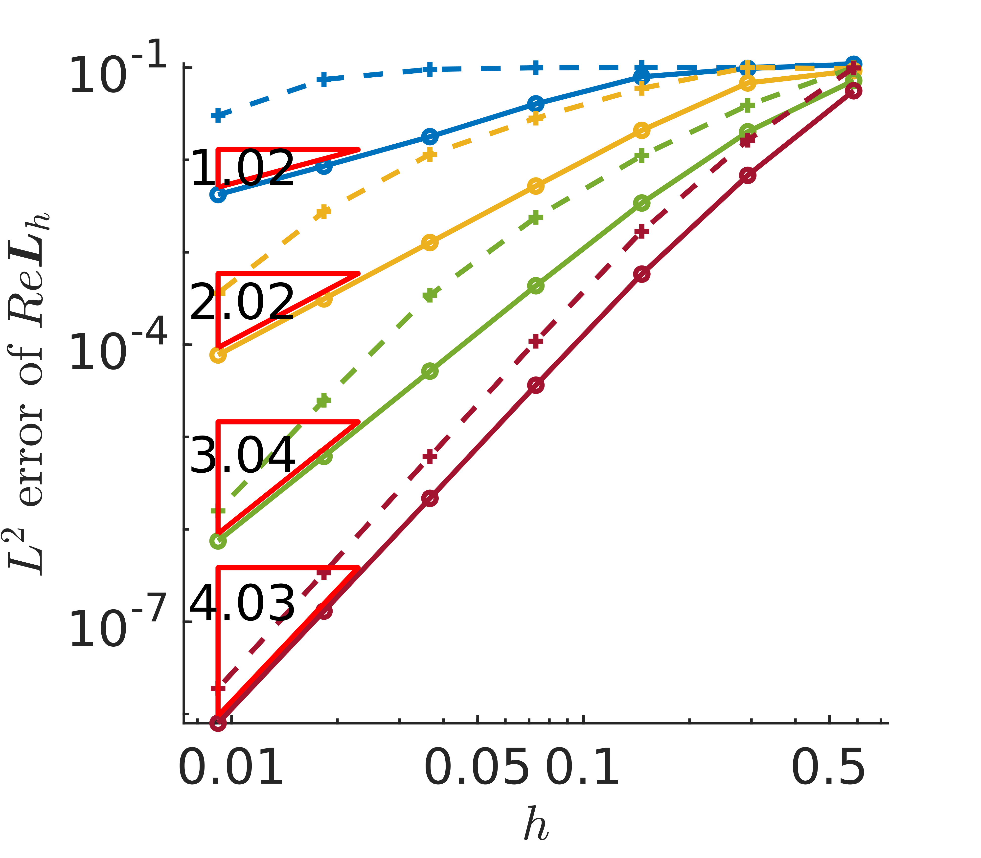
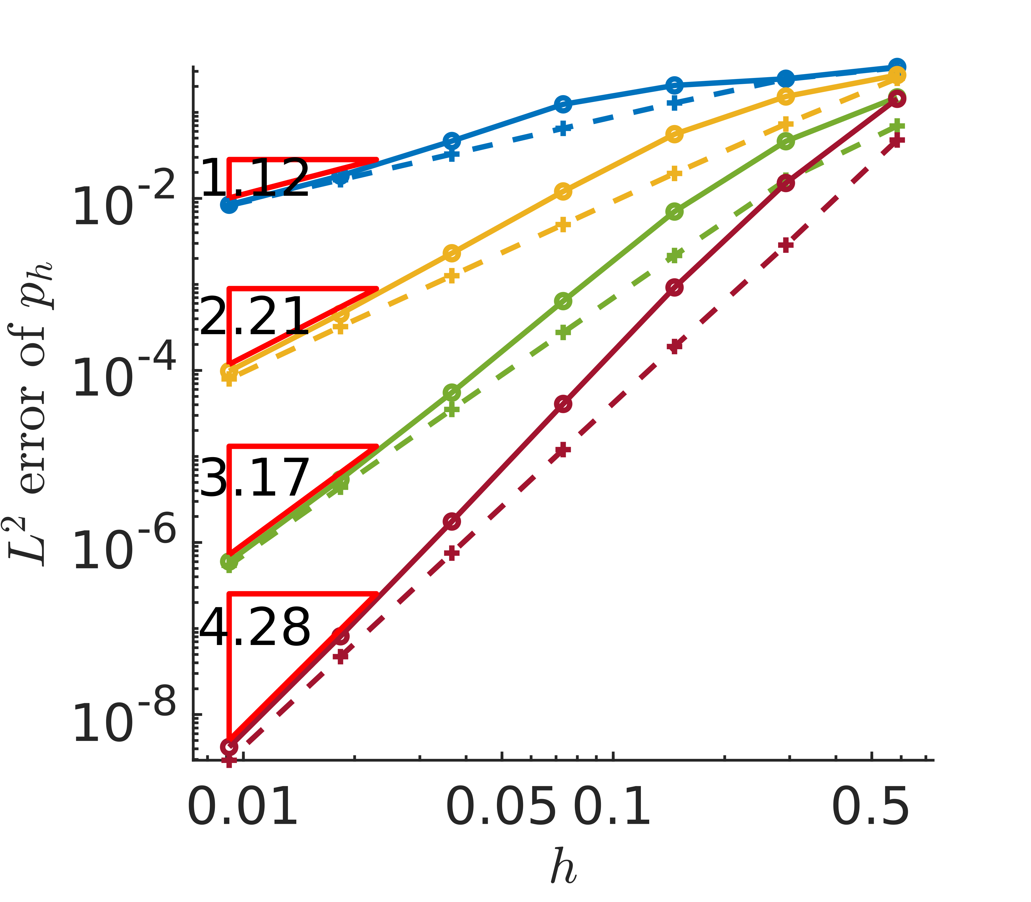
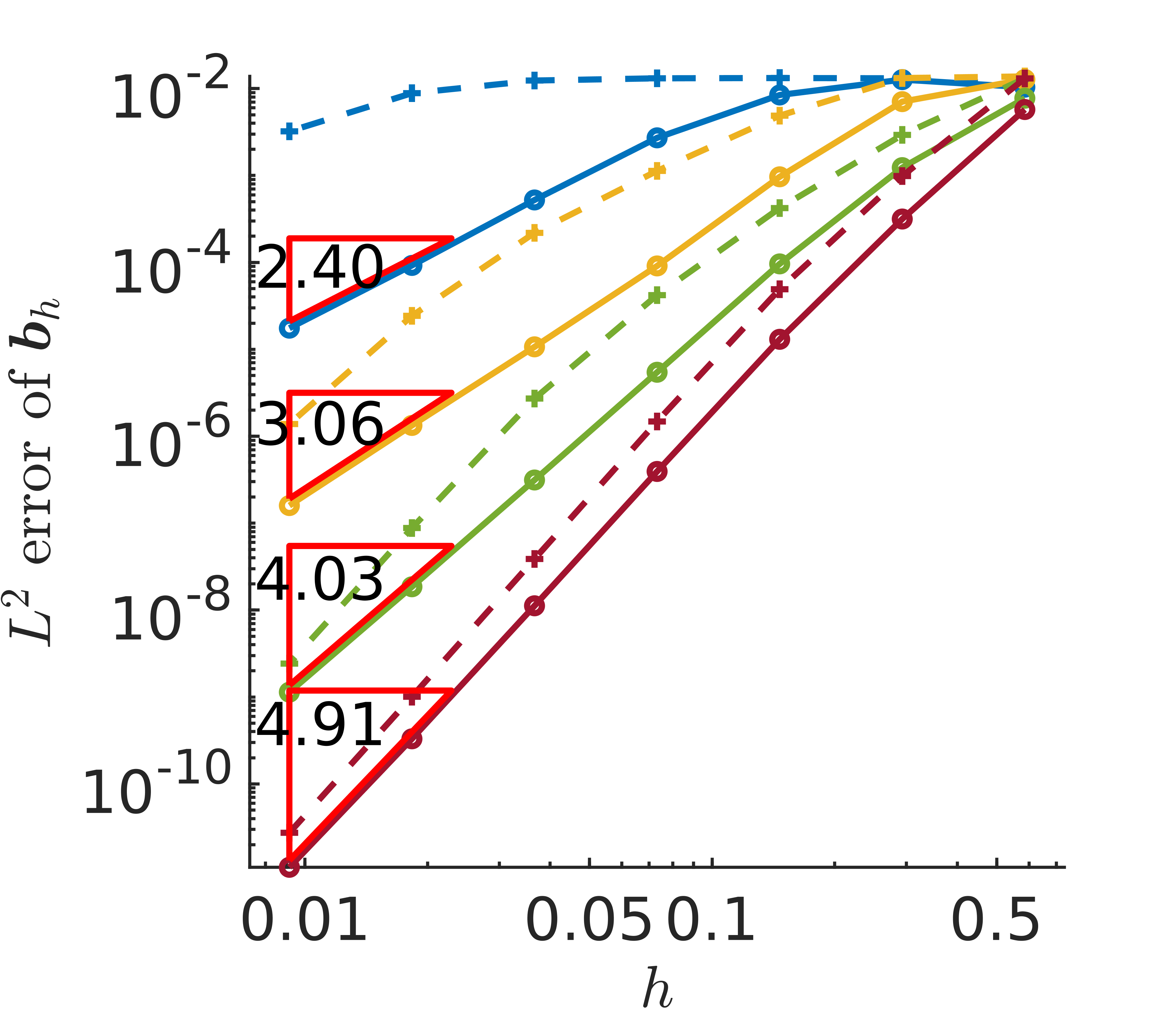
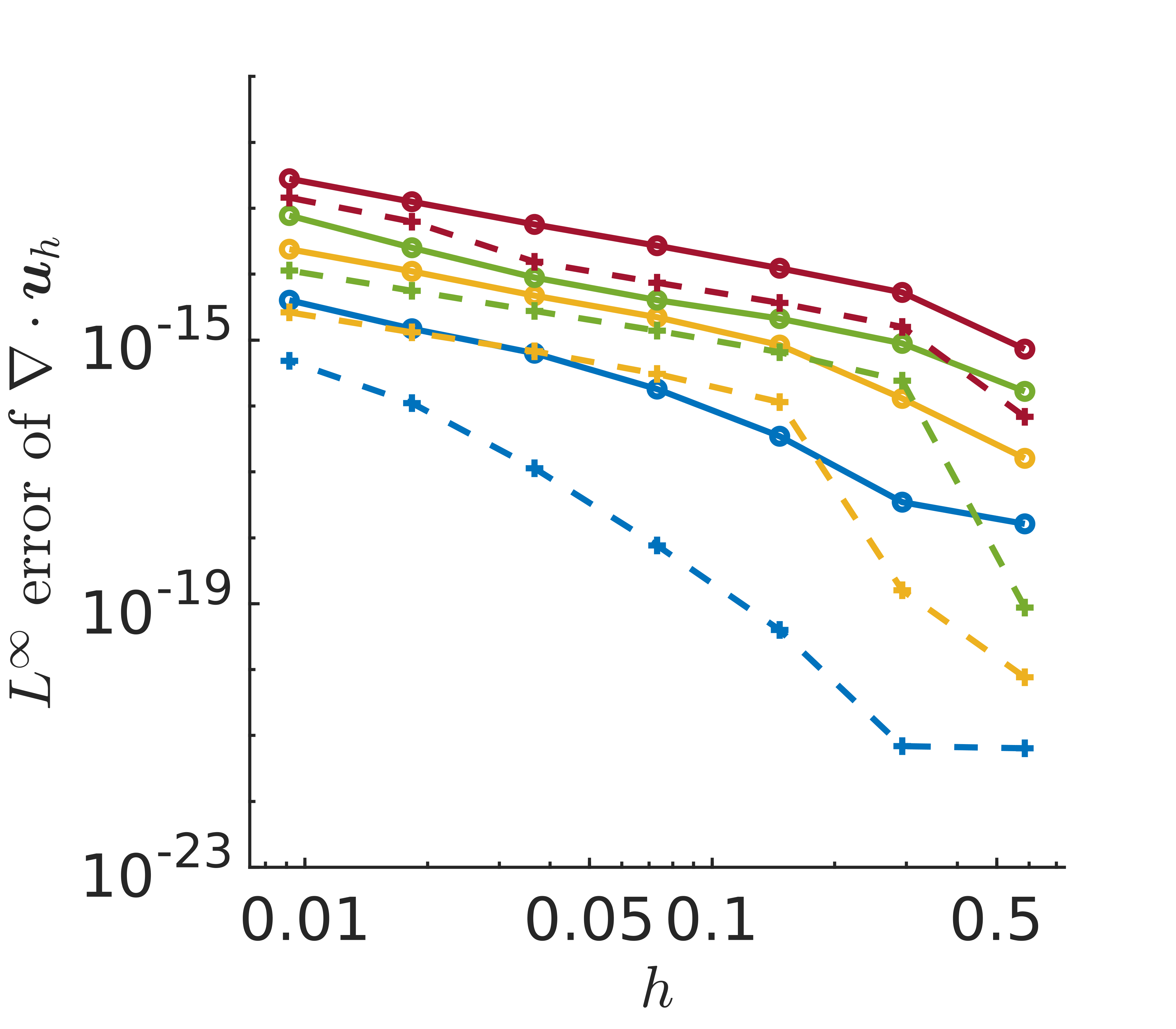
Figure 1: Convergence histories of all local variables and divergence errors for the E-HDG method applied to solve the two-dimensional problem with a smooth manufactured solution given in (28) where we set ${p}_{0}=1$. Only the convergence rates for $\textup{Re}=\textup{Rm}=1$ are presented here.

4.2.2 Two-dimensional singular manufactured solution

To assess the robustness of our E-HDG scheme, it is applied to solve the problem where a strong singularity exists on the boundary. The example illustrates the convergence of the E-HDG scheme using a manufactured solution with a singularity (similar to the example in Section 5.2 of [55] and Section 5.3 of [67]). In particular, we consider the nonconvex domain $\Omega=(-1,1)\times(-1,1)\backslash[0,1)\times(-1,0]$. We take $\textup{Re}=\textup{Rm}=\kappa=1$, $\boldsymbol{w}=\boldsymbol{0}$, and $\boldsymbol{{d}}=(-1,1)$. We pick $\boldsymbol{g}$ and $\boldsymbol{f}$ such that the analytical solution of (3)-(5) has the form

(29a) $$\begin{split}\boldsymbol{u}=\begin{pmatrix}\rho^{\lambda}\left[(1+\lambda)\sin{(\phi)}\psi(\phi)+\cos{(\phi)}\psi^{\prime}(\phi)\right],\\ \rho^{\lambda}\left[-(1+\lambda)\cos{(\phi)}\psi(\phi)+\sin{(\phi)}\psi^{\prime}(\phi)\right]\end{pmatrix},\end{split}$$

(29b) $$\begin{split}\boldsymbol{b}=\nabla{\left(\rho^{2/3}\sin{\left(\frac{2\phi}{3}\right)}\right)},\end{split}$$

(29c) $$\begin{split}{p}=-\rho^{\lambda-1}\frac{\left(1+\lambda\right)^{2}\psi^{\prime}(\phi)+\psi^{\prime\prime\prime}(\phi)}{1-\lambda},\end{split}$$

(29d) $$\begin{split}r=0,\end{split}$$

where

$$\psi(\phi)=\cos{(\lambda\omega)}\left[\frac{\sin{\left((1+\lambda)\phi\right)}}{1+\lambda}-\frac{\sin{\left((1-\lambda)\phi\right)}}{1-\lambda}\right]-\cos{\left((1+\lambda)\phi\right)}+\cos{\left((1-\lambda)\phi\right)},$$

$$\omega=\frac{3\pi}{2},\quad\lambda\approx 0.54448373678246,\quad\phi\in\left[0,\frac{3\pi}{2}\right].$$

For this problem, it is known that $\boldsymbol{u}\in\left[H^{1+\lambda}(\Omega)\right]^{2}$, ${p}\in H^{\lambda}(\Omega)$, and $\boldsymbol{b}\in\left[H^{2/3}(\Omega)\right]^{2}$, and the solution contains magnetic and hydrodynamic singularities that are among the strongest singularities [55].

Convergence results for this problem are summarized in Table 6 and shown in Figure 2. For the fluid variables $\boldsymbol{L}_{h}$, $\boldsymbol{u}_{h}$, and $p_{h}$, we observe convergence rates of approximately 2/3. For the magnetic variables $\boldsymbol{J}_{h}$, $\boldsymbol{b}_{h}$, and $r_{h}$, we observe convergence rates of approximated 1/5, 2/3, and 1/3 respectively. Compared to the result presented in [67], the convergence rates of the fluid variables are worse while the ones of the magnetic variables are similar. Remarkably, the divergence errors in both velocity and magnetic field are still close to machine zero in this singular problem.

In terms of accuracy, our E-HDG method is much worse than the HDG method presented in [67]. The reason behind this is that the singular point $(0,0)$ has to be explicitly evaluated for enforcing the Dirichlet boundary condition in the E-HDG method in which a continuous function basis for the global variable $\hat{\boldsymbol{b}}_{h}$ is used and a quadrature point coincide with the singular point $(0,0)$ that also acts as a nodal point. Such an obstacle can be circumvented by using a discontinuous function basis along with Gauss quadrature. Indeed, we observed a similar level of accuracy compared to the result in [67] when switching our E-HDG method to the HDG method (not shown here).

$\textup{Re}=\textup{Rm}=\kappa=1$
	$\textup{Re}\boldsymbol{L}_{h}$	$\boldsymbol{u}_{h}$	$p_{h}$	$\frac{\textup{Rm}}{\kappa}\boldsymbol{J}_{h}$	$\boldsymbol{b}_{h}$	$r_{h}$	$\left\lVert\nabla\cdot{\boldsymbol{u}_{h}}\right\rVert_{\infty}$	$\left\lVert\nabla\cdot{\boldsymbol{b}_{h}}\right\rVert_{\infty}$
$k=1$	0.64	0.64	0.65	0.09	0.68	0.46	1.70E-12	3.82E-11
$k=2$	0.63	0.63	0.65	0.12	0.65	0.31	7.57E-12	3.78E-10
$k=3$	0.65	0.67	0.69	0.20	0.64	0.32	1.68E-11	8.57E-10
$k=4$	0.66	0.68	0.71	0.26	0.62	0.36	3.68E-11	4.26E-09

Table 6: Convergence rates of all local variables and divergence errors of velocity and magnetic fields for the E-HDG method applied to solve the two-dimensional problem with a singular manufactured solution given in (29). The corresponding results are also presented in Figure 2. In this table, the convergence rates are evaluated at the last two data sets and the divergence errors are evaluated at the last data set.

Figure 2: Convergence histories of all local variables and divergence errors for the E-HDG method applied to solve the two-dimensional problem with a manufactured solution given in (29) where a strong singularity exists in the magnetic field.

4.2.3 Three-dimensional smooth manufactured solution

We now apply our E-HDG method to a three-dimensional problem on structured tetrahedron meshes. Note that our well-posedness analysis is still valid for this case. We set $\Omega=(0,1)\times(0,1)\times(0,1)$ and take $\textup{Re}=\textup{Rm}\in\left\{1,1000\right\}$ and $\kappa=1$. In this testing case, we choose the forcing function such that the exact solution is given by

(30a) $$\begin{split}\boldsymbol{u}=\begin{pmatrix}-\left(y\cos{(y)}+\sin{y}\right)e^{x},\\ y\sin{(y)}e^{x}-\left(z\cos{(z)}+\sin{(z)}\right)e^{y},\\ z\sin{(z)}e^{y}\end{pmatrix},\end{split}$$

(30b) $$\begin{split}\boldsymbol{b}=\boldsymbol{u}\end{split}$$

(30c) $$\begin{split}{p}={p}_{0}\left(2E^{x}\sin{(y)}z^{2}-\left(\frac{-2}{3}(e\cos{(1)}-\cos{(1)}-e+1\right)\right)\end{split}$$

(30d) $$\begin{split}r=0\end{split}$$

with the prescribed fields $\boldsymbol{w}=\boldsymbol{u}$ and $\boldsymbol{{d}}=\boldsymbol{b}$, and a constant ${p}_{0}$. Table 7 summarizes the convergence rates of all local variables along with the divergence errors measured in $L^{\infty}$-norm. The corresponding convergence histories are shown in Figure 3. Similar to the two-dimensional smooth testing case presented in Section 4.2.1, we observed that the convergence rates are affected by Re and Rm here as well but in an adverse manner. The effect is evident in $\boldsymbol{L}_{h}$, $\boldsymbol{u}_{h}$ and $\boldsymbol{b}_{h}$. Given that the result of $\textup{Re}=\textup{Rm}=1000$ is somehow irregular, we derive the convergence rates from the testing case of $\textup{Re}=\textup{Rm}=1$. As can be seen, $p_{h}$ and $r_{h}$ exhibit superconvergence with a rate of $\overline{k}+3/2$, and the convergence rates of ${\hat{\boldsymbol{u}}}$ and $\boldsymbol{b}_{h}$ are optimal with $k+1$. For $\boldsymbol{L}_{h}$ and $\boldsymbol{J}_{h}$, the convergence rate is, however, suboptimal with $k$. The conclusion is consistent with the one made in Section 4.2.1 where the two-dimensional smooth manufactured solution is applied.

The numerical assessment of the pressure robustness of our method is also carried out for a three-dimensional setting in this section. We solved the manufactured solution problem using meshes of 48 elements and 24576 elements, a polynomial degree of $k=2$, and a range of ${p}_{0}$. Table 8 shows the results. Similar to the two-dimensional case displayed in Table 5, we observe that the $L^{2}$-errors in velocity and magnetic field are independent of the $L^{2}$-error in pressure on different meshes.

$\textup{Re}=\textup{Rm}=1,\kappa=1$
	$\textup{Re}\boldsymbol{L}_{h}$	$\boldsymbol{u}_{h}$	$p_{h}$	$\frac{\textup{Rm}}{\kappa}\boldsymbol{J}_{h}$	$\boldsymbol{b}_{h}$	$r_{h}$	$\left\lVert\nabla\cdot{\boldsymbol{u}_{h}}\right\rVert_{\infty}$	$\left\lVert\nabla\cdot{\boldsymbol{b}_{h}}\right\rVert_{\infty}$
$k=1$	0.72	1.78	1.81	1.02	2.04	1.95	6.19E-13	2.11E-13
$k=2$	2.21	3.50	2.85	2.21	3.23	2.79	1.41E-12	1.29E-12
$k=3$	3.08	3.99	3.66	3.22	4.19	3.75	9.07E-10	1.96E-11
$k=4$	4.22	5.23	4.73	4.24	5.23	4.70	3.66E-09	8.06E-11
$\textup{Re}=\textup{Rm}=1000,\kappa=1$
$k=1$	0.47	1.38	1.89	0.56	0.77	1.96	5.73E-13	2.13E-13
$k=2$	1.28	2.25	3.01	1.31	2.19	2.93	1.64E-12	1.45E-12
$k=3$	3.64	4.69	3.92	3.77	4.72	3.93	1.46E-09	1.93E-11
$k=4$	3.94	4.22	4.91	4.03	4.29	5.49	5.55E-09	5.94E-09

Table 7: Convergence rates of all local variables and divergence errors of velocity and magnetic fields for the E-HDG method applied to solve the three-dimensional problem with a smooth manufactured solution given in (30) where we set ${p}_{0}=1$. The corresponding results are also presented in Figure 3. In this table, the convergence rates are evaluated at the last two data sets and the divergence errors are evaluated at the last data set.

48 elements in total, $h\approx 1.06E-1$
$p_{0}$	$\textup{Re}\left\lVert\boldsymbol{L}-\boldsymbol{L}_{h}\right\rVert_{0}$	$\left\lVert\boldsymbol{u}-\boldsymbol{u}_{h}\right\rVert_{0}$	$\left\lVert{p}-p_{h}\right\rVert_{0}$	$\frac{\textup{Rm}}{\kappa}\left\lVert\boldsymbol{J}-\boldsymbol{J}_{h}\right\rVert_{0}$	$\left\lVert\boldsymbol{b}-\boldsymbol{b}_{h}\right\rVert_{0}$	$\left\lVert r-r_{h}\right\rVert_{0}$	$\left\lVert\nabla\cdot{\boldsymbol{u}_{h}}\right\rVert_{\infty}$	$\left\lVert\nabla\cdot{\boldsymbol{b}_{h}}\right\rVert_{\infty}$
1	7.52E-2	2.69E-3	1.59	6.42E-2	2.42E-3	1.29	2.42E-13	2.19E-13
10	7.52E-2	2.69E-3	5.99	6.42E-2	2.42E-3	1.29	2.99E-13	2.48E-13
25	7.52E-2	2.69E-3	15.57	6.42E-2	2.42E-3	1.29	3.09E-13	2.53E-13
100	7.52E-2	2.69E-3	64.09	6.42E-2	2.42E-3	1.29	2.89E-13	2.60E-13
24576 elements in total, $h\approx 2.64E-2$
1	3.19E-3	2.10E-5	3.16E-2	2.70E-3	2.53E-5	2.90E-2	1.40E-12	1.43E-12
10	3.19E-3	2.10E-5	5.83	2.70E-3	2.53E-5	2.90E-2	1.40E-12	1.31E-12
25	3.19E-3	2.10E-5	15.55	2.70E-3	2.53E-5	2.90E-2	1.41E-12	1.22E-12
100	3.19E-3	2.10E-5	64.13	2.70E-3	2.53E-5	2.90E-2	1.32E-12	1.44E-12

Table 8: The errors in the local variables for the smooth manufactured solution given in (30) for meshes of 48 and 24576 elements, a polynomial degree of $k=2$, and a range of $p_{0}$ values. The physical parameters are set to be $\textup{Re}=\textup{Rm}=1$ and $\kappa=1$.

Figure 3: Convergence histories of all local variables and divergence errors for the E-HDG method applied to solve the three-dimensional problem with a smooth manufactured solution given in (30) where we set ${p}_{0}=1$. Only the convergence rates for $\textup{Re}=\textup{Rm}=1$ are presented here.

4.3 Nonlinear examples

To verify our nonlinear solver, we conducted several numerical experiments and studied the accuracy and convergence. The first example is the two-dimensional smooth manufactured solution, the second one is the so-called Hartmann flow problem, and the last one is the three-dimensional smooth manufactured solution.

4.3.1 Two-dimensional smooth manufactured solution

Our first numerical experiment for the nonlinear solver is a steady manufactured solution. In particular, we use the same solution presented in Section 4.2.1 to investigate the convergence. The results are concluded in Table 9 and are illustrated in Figure 4. The observed convergence rates are almost the same as the rates observed in the linear problem presented in Section 4.2.1. Moreover, the divergence errors have the same order of magnitude in both tables.

$\textup{Re}=\textup{Rm}=1,\kappa=1$
	$\textup{Re}\boldsymbol{L}_{h}$	$\boldsymbol{u}_{h}$	$p_{h}$	$\frac{\textup{Rm}}{\kappa}\boldsymbol{J}_{h}$	$\boldsymbol{b}_{h}$	$r_{h}$	$\left\lVert\nabla\cdot{\boldsymbol{u}_{h}}\right\rVert_{\infty}$	$\left\lVert\nabla\cdot{\boldsymbol{b}_{h}}\right\rVert_{\infty}$
$k=1$	1.02	2.29	1.12	1.20	2.40	1.96	4.02E-15	3.72E-15
$k=2$	2.02	3.08	2.21	2.28	3.06	2.73	2.39E-14	2.66E-14
$k=3$	3.04	4.06	3.17	3.35	4.03	3.75	7.75E-14	7.65E-14
$k=4$	4.03	5.08	4.28	4.51	4.91	4.79	2.81E-13	5.65E-13
$\textup{Re}=\textup{Rm}=1000,\kappa=1$
$k=1$	1.27	1.35	0.99	1.38	1.47	0.65	2.69E-15	2.83E-15
$k=2$	2.93	4.04	2.02	3.01	4.14	2.40	2.61E-14	2.35E-14
$k=3$	3.98	5.28	3.02	3.85	5.18	3.81	1.13E-12	1.10E-13
$k=4$	4.16	5.20	4.00	4.17	5.20	4.39	2.78E-12	1.73E-12

Table 9: Convergence rates of all local variables and divergence errors of velocity and magnetic fields for the nonlinear solver applied to solve the two-dimensional problem with a smooth manufactured solution given in (28) where we set ${p}_{0}=1$. The corresponding results are also presented in Figure 4. In this table, the convergence rates are evaluated at the last two data sets and the divergence errors are evaluated at the last data set.

Figure 4: Convergence histories of all local variables and divergence errors for the nonlinear solver applied to solve the two-dimensional problem with a smooth manufactured solution given in (28) where we set ${p}_{0}=1$. Only the convergence rates for $\textup{Re}=\textup{Rm}=1$ are presented here.

4.3.2 Two-dimensional Hartmann flow

We next consider the Hartmann channel flow, a generalization of the classic plane Poiseuille problem to the setting of the incompressible resistive MHD. In this problem, a conducting incompressible fluid (liquid metal, for example) in a domain $(-\infty,\infty)\times(-l_{0},l_{0})\times(-\infty,\infty)$ (bounded by infinite parallel plates in the $x_{2}$ direction) is driven by a uniform pressure gradient $G:=-\frac{\partial{p}}{\partial x_{1}}$ in the $x_{1}$ direction, and is subject to a uniform external magnetic field $b_{0}$ in the $x_{2}$ direction. In addition, we enforce no-slip boundary conditions on the $x_{2}$ boundaries and assume the infinite parallel plates are perfectly insulating. The resulting flow pattern admits an analytical solution that is one dimension in nature. In this numerical study, we consider the simulation of Hartmann flow in a two-dimensional domain $\Omega=(0,0.025)\times(-1,1)$. If we define the characteristic velocity as $u_{0}:=\sqrt{Gl_{0}/\rho}$ and consider the driving pressure gradient $G$ as a forcing term (incorporated in $\boldsymbol{g}$), the nondimensionalized solution with $\boldsymbol{g}=(1,0)$, $\boldsymbol{f}=\boldsymbol{0}$ takes the form (see, i.e., [85, 86])

(31a) $$\begin{split}\boldsymbol{u}=\left(\frac{\textup{Re}}{Ha\tanh{(Ha)}}\left[1-\frac{\cosh{(Ha\cdot y)}}{\cosh{(Ha)}}\right],0\right),\end{split}$$

(31b) $$\begin{split}\boldsymbol{b}=\left(\frac{1}{\kappa}\left[\frac{\sinh{(Ha\cdot y)}}{\sinh{(Ha)}}-y\right],1\right),\end{split}$$

(31c) $$\begin{split}{p}=-\frac{1}{2\kappa}\left[\frac{\sinh{(Ha\cdot y)}}{\sinh{(Ha)}}-y\right]^{2}-{p}_{0},\end{split}$$

(31d) $$\begin{split}r=0\end{split}$$

where $Ha:=\sqrt{\kappa\textup{Re}\textup{Rm}}$, and ${p}_{0}$ is a constant that enables ${p}$ to satisfy the zero average pressure condition.

At refinement level $l$, the domain is divided into $l\times 80l$ squares, each of which is divided into two triangles from top right to bottom left. Figure 5 shows the convergence plots with $\textup{Re}=\textup{Rm}=7.07$ and $\kappa=200$ and the corresponding convergence rates are summarized in Table 10. The convergence rates for $\boldsymbol{L}_{h}$, $\boldsymbol{u}_{h}$, $p_{h}$, $\boldsymbol{J}_{h}$, $\boldsymbol{b}_{h}$, and $r_{h}$ are observed to be approximately $k$, $k-1/2$, $\overline{k}+1$, $k$, $k+1/2$, and $\overline{k}+1$. The observation is mostly consistent with the rates observed in Section 4.2.1 and 4.2.3 except for the ones of the velocity and magnetic fields, which are sub-optimal here.

$\textup{Re}=\textup{Rm}=7.07,\kappa=200$
	$\textup{Re}\boldsymbol{L}_{h}$	$\boldsymbol{u}_{h}$	$p_{h}$	$\frac{\textup{Rm}}{\kappa}\boldsymbol{J}_{h}$	$\boldsymbol{b}_{h}$	$r_{h}$	$\left\lVert\nabla\cdot{\boldsymbol{u}_{h}}\right\rVert_{\infty}$	$\left\lVert\nabla\cdot{\boldsymbol{b}_{h}}\right\rVert_{\infty}$
$k=1$	1.01	3.68	1.01	1.03	1.87	1.26	3.52E-09	5.50E-12
$k=2$	2.08	1.81	2.03	1.96	2.58	1.74	2.95E-08	1.28E-10
$k=3$	3.20	2.59	3.16	3.55	3.64	3.18	1.30E-07	2.90E-10
$k=4$	4.17	3.72	4.13	4.21	4.20	3.96	3.16E-07	7.02E-10

Table 10: Convergence rates of all local variables and divergence errors of velocity and magnetic fields for the nonlinear solver applied to solve the two-dimensional Hartmann flow problem that admits the solution given in (31). The corresponding results are also presented in Figure 5. In this table, the convergence rates are evaluated at the last two data sets and the divergence errors are evaluated at the last data set.

Figure 5: Convergence histories of all local variables and divergence errors for the nonlinear solver applied to solve the two-dimensional Hartmann flow problem that admits the solution given in (31).

4.3.3 Three-dimensional smooth manufactured solution

We finally consider the three-dimensional nonlinear problem. The example demonstrates the convergence of the nonlinear solver using a smooth three-dimensional smooth manufactured solution that is the same as the one presented in Section 4.2.3. The numerical results are concluded in Table 11 and demonstrated in Figure 11. The observed convergence rates are consistent with the rates presented in Section 4.3.3 where a linear problem with the same smooth manufactured solution is solved. Particularly, Table 11 is almost identical to Table 7. In addition, the same order of magnitude is observed in both tables for the divergence errors.

However, it is well known that the Picard solver does not necessarily converge, and whether the iteration converges or not depends on the initial guess. Moreover, we found that the convergence of the Picard solver is substantially influenced by the physical parameters $\textup{Re},\textup{Rm}$, the degree of approximation $k$, and the refinement of mesh. Particularly, in the testing cases with $\textup{Re}=\textup{Rm}=1000$ and $k>1$, the Picard iteration does not converge using the initial guess $\boldsymbol{u}_{h}^{0}=\boldsymbol{b}_{h}^{0}=\boldsymbol{0}$. By taking $\textup{Re}=\textup{Rm}=1000$, the Picard iteration begins to stall when $k=2$ is applied on the mesh of 364 elements, $k=3$ is applied on the mesh of 48 elements, and $k=4$ is applied on the mesh of 6 elements. Only the case with $k=1$ does converge on a sequence of meshes with 6, 48, 364, 3072, and 24576 elements, and the result of this case is also presented in Table 11 and in Figure 11.

$\textup{Re}=\textup{Rm}=1,\kappa=1$
	$\textup{Re}\boldsymbol{L}_{h}$	$\boldsymbol{u}_{h}$	$p_{h}$	$\frac{\textup{Rm}}{\kappa}\boldsymbol{J}_{h}$	$\boldsymbol{b}_{h}$	$r_{h}$	$\left\lVert\nabla\cdot{\boldsymbol{u}_{h}}\right\rVert_{\infty}$	$\left\lVert\nabla\cdot{\boldsymbol{b}_{h}}\right\rVert_{\infty}$
$k=1$	0.72	1.78	1.81	1.02	2.04	1.95	6.89E-13	2.97E-13
$k=2$	2.21	3.50	2.85	2.21	3.23	2.78	1.37E-12	1.37E-12
$k=3$	3.08	3.99	3.66	3.22	4.19	3.75	9.32E-10	2.07E-11
$k=4$	4.22	5.23	4.73	4.24	5.23	4.70	3.47E-09	8.38E-11
$\textup{Re}=\textup{Rm}=1000,\kappa=1$
$k=1$	0.47	1.36	1.89	0.57	0.80	1.96	6.08E-13	2.47E-13

Table 11: Convergence rates of all local variables and divergence errors of velocity and magnetic fields for the nonlinear solver applied to solve the three-dimensional problem with a smooth manufactured solution given in (30) where we set ${p}_{0}=1$. The corresponding results are also presented in Figure 6. In this table, the convergence rates are evaluated at the last two data sets and the divergence errors are evaluated at the last data set.

Figure 6: Convergence histories of all local variables and divergence errors for the nonlinear solver applied to solve the three-dimensional problem with a smooth manufactured solution given in (30) where we set ${p}_{0}=1$. Only the convergence rates for $\textup{Re}=\textup{Rm}=1$ are presented here.

5 Conclusion

In this paper, we proposed an E-HDG method for linearization of the incompressible viso-resistive MHD equations and carried out the well-posedness analysis. Particularly, we showed that on a simplicial mesh the well-posedness of our method can be guaranteed by (i) an order lower approximation in local pressure $p_{h}$ and Lagrange multiplier $r_{h}$, and (ii) suitable stabilization parameters. Furthermore, the divergence constraints on velocity and magnetic fields are proved to be satisfied pointwisely and globally. Hence, our proposed method is automatically divergence-conforming. Additionally, all results can be applied to the HDG version of our proposed approach. One of the motivations for considering E-HDG in lieu of HDG methods lies in computational performance. Indeed, we see a significant acceleration in execution time, which is reflected by the fewer DOFs used in the E-HDG method in the testing cases where the linear solver dominates total computational time (i.e., three dimensions with a high-order approximation on a fine mesh). Linear problems with both smooth and singular solutions are presented to examine the convergence of the proposed E-HDG method. For problems with smooth solutions, both two- and three-dimensional settings are tested. The numerical convergence rates are shown to be optimal for both velocity and magnetic fields in the regime of low Reynolds number and magnetic Reynolds number. Moreover, our method is numerically verified to be pressure-robust. For the singular solution, the convergence rate is limited by the regularity of the solution. However, the divergence-conforming property is still numerically observed. By incorporating the E-HDG discretization into the fixed point Picard iteration, we can solve the full nonlinear incompressible viso-resistive MHD equations in an iterative manner. Moreover, both velocity and magnetic fields are still globally pointwise divergence-free. The convergence of the nonlinear solver is investigated through nonlinear problems with smooth solutions. It is found that the Picard solver does not converge in some cases on three-dimensional meshes in the regime of high Reynolds number and magnetic Reynolds number. Otherwise, the convergence rates are almost identical to the ones observed in the linear tests of both two- and three-dimensional settings. In addition, divergence errors in both velocity and magnetic fields are indeed observed to be machine zero.