Assurance methods for designing a clinical trial with a delayed treatment effect

Abstract

An assurance calculation is a Bayesian alternative to a power calculation. One may be performed to aid the planning of a clinical trial, specifically setting the sample size or to support decisions about whether or not to perform a study. Immuno-oncology (IO) is a rapidly evolving area in the development of anticancer drugs. A common phenomenon that arises from IO trials is one of delayed treatment effects, that is, there is a delay in the separation of the survival curves. To calculate assurance for a trial in which a delayed treatment effect is likely to be present, uncertainty about key parameters needs to be considered. If uncertainty is not considered, then the number of patients recruited may not be enough to ensure we have adequate statistical power to detect a clinically relevant treatment effect. We present a new elicitation technique for when a delayed treatment effect is likely to be present and show how to compute assurance using these elicited prior distributions. We provide an example to illustrate how this could be used in practice. Open-source software is provided for implementing our methods. Our methodology makes the benefits of assurance methods available for the planning of IO trials (and others where a delayed treatment expect is likely to occur).

, , and (<year>), <journal title>, <journal name> <year> <vol> Page <xxx>-<xxx>

1 Introduction

Assurance calculations are growing in popularity as an aid for the design of clinical trials. An assurance calculation is a Bayesian alternative to a classical frequentist power calculation: instead of assuming parameters take particular values, we now assume prior distributions for them, thus incorporating uncertainty. The concept of an assurance calculation was first considered by Spiegelhalter and Freedman¹, then developed by O’Hagan et al², who coined the term ‘assurance’. Note that the assurance method has had other terms accredited to it, such as average power, expected power and predictive power³. When calculating assurance, first prior distributions for unknown parameters are sampled from and then clinical trials are simulated using these sampled values, with the prior predictive probability that the trial will be ‘successful’ being the proportion of the simulated trials that meet our stated success criteria. These success criteria are not fixed by the assurance method; instead, they are set independently by the sponsor and can be any criteria that the sponsor wishes to consider (eg, that the observed treatment effect will be positive, statistically significant at the appropriate size and exceed a clinically relevant threshold). More recently, assurance has been used in the wider context of calculating the probability of success (PoS) for a future Phase III trial, usually after a Phase IIb trial^{4, 5}; other authors have calculated the probability of obtaining regulatory approval with clinically relevant effects on key endpoints after Phase IIb^{6, 7}. Note that the proposed trial need not be analysed using Bayesian methods (although this is still possible).

Assurance provides a more realistic assessment of the probability a trial will give rise to a ‘successful’ outcome, compared to a conventional power calculation. The high failure rates of clinical trials are well-documented⁸, and there are several examples where promising results from small early phase trials have not been replicated in larger subsequent Phase III trials⁹. Assurance calculations for Phase III trials should capture the strength of the available evidence after mitigating the selection bias often inherent in early phase data when a necessary condition for progress is positive Phase Ib or Phase II results, and also accounting for any limitations in the available data in light of planned shifts in the patient population, outcome and treatment between phases. Accurate and reliable evaluations of risk can be used to optimize trial design and analysis plans. For example, assurance can be used to support decisions regarding study sample size, and quantitatively measure how effective various trial setups are at reducing risks, such as the timing and number of planned interim analyses^{10, 4}. Furthermore, assurance evaluations can also enable better informed go/no-go decisions regarding study conduct. Of course sponsors, such as pharmaceutical companies and public funding bodies, may choose to fund a pivotal clinical trial (or indeed a program of pivotal clinical trials) regardless of whether it has a low assurance if the corresponding expected net present value (eNPV) is sufficiently high, thus targeting resources towards research programs with the greatest expected impact for patients.

Immuno-oncology (IO) is a rapidly evolving area in the development of anticancer drugs. In trials of IO therapies, non constant treatment effects violating the proportional hazards (PH) assumption have been observed on time-to-event endpoints such as progression-free survival (PFS) and overall survival (OS). See for example, CheckMate 017¹². In a systematic review of 63 pivotal randomized controlled trials (RCTs) of anti-programmed cell death protein-1 and anti-programmed death/ligand 1 therapies¹³, 15 studies were identified with suspected nonproportional hazards due to reasons including crossing of the OS survival curves^{14, 15} or a delay in the separation of the PFS survival curves¹⁶. In what follows, we focus on the latter scenario and refer to this as a delayed treatment effect (DTE). There are several challenges associated with the design and analysis of trials with nonproportional hazards. Firstly, the primary estimand should be defined with a clinically interpretable measure used to summarize the benefit of the test treatment versus control¹⁷, and an unbiased estimator should be selected to target it. Secondly, the test of the null hypothesis of no benefit of treatment versus control should be carefully selected acknowledging the impact of potential deviations from PH on the attained power of commonly applied procedures, such as the log-rank test¹¹. When planning a trial where we suspect (but are not certain) that there will be a delay in the treatment effect, and furthermore are uncertain about the length of the delay if there is one, the target event number and corresponding sample size needs to be carefully chosen to provide confidence it will be able to meet its objectives in light of these uncertainties.

As IO trials are becoming more common, so are trials in which a DTE is observed. However, to the best of our knowledge, there has been no published work on eliciting prior distributions and calculating assurance for when a DTE is likely to be present in a clinical trial with time-to-event endpoints. In this article, we propose a method for how to elicit the relevant parameters for this trial and how to perform an assurance calculation.

In Section 2, we briefly discuss the assurance method and how it is being used in practice. In Section 3, we introduce DTEs and present an elicitation method for this situation. In Section 5, we illustrate how our method can be used to calculate assurance. In Section 6, we investigate the robustness of our parameterisation and lastly we conclude with a brief summary in Section 7. Free software for implementing our methods is found in the Appendix.

2 Assurance

Suppose that a randomised controlled trial (RCT) is to be conducted to compare an experimental treatment with a control intervention (we assume that this is the current standard of care, but could also be a placebo). A hypothesis test is to be carried out to test the null hypothesis $H_{0}$ that the treatment effect $\theta=0$ versus the alternative hypothesis $H_{1}$ that $\theta\neq 0$. For a power calculation, the sample size is chosen to solve

$$P(\text{Reject }H_{0}|\theta=\theta_{A})=\pi^{*},$$ (1)

for some desired probability $\pi^{*}$ (usually 80% or 90%) and a minimum clinically relevant treatment effect $\theta_{A}$.

The power of the test of $H_{0}$ at $\theta_{A}$ represents the probability of rejecting $H_{0}$ if the true value of $\theta$ is as large as $\theta_{A}$. However, since the true value of $\theta$ may differ from $\theta_{A}$, the attained power of the test may deviate from the target $\pi^{\star}$. Assurance is the unconditional probability that the trial will end with the desired outcome, which can be derived via

$$P(\text{`Successful trial'})=\int P(\text{`Successful trial'}|\theta)f(\theta)\text{d}(\theta),$$ (2)

where $f(\theta)$ is the prior distribution for the true treatment effect $\theta$. If a successful trial simply corresponds to rejecting $H_{0}$, Equation 2 is the expected power, interpreting $\theta_{A}$ in Equation 1 as the true value of the treatment effect, rather than some minimum clinically relevant difference.

If the desired outcome is to reject $H_{0}$ with data which favours the experimental treatment, then the event ‘successful trial’ may be defined as ‘Reject $H_{0}$ with $\hat{\theta}>0$’. When calculating assurance, a key question is how to define the prior distribution $f(\theta)$ for the unknown treatment effect. One approach would be to take $f(\theta)$ as the posterior distribution for $\theta$ resulting from using clinical data from an early Phase II trial to update a weakly informative prior distribution. However, this approach may fail to incorporate other sources of relevant information, and may become challenging if there are differences between the treatment effect studied in Phase II and the quantity of interest in the future trial. Alternatively, the prior distribution(s) for the parameters of interest could be elicited from a group of experts, in light of the Phase IIb trial data, and any other information that is deemed relevant – data from drugs with a similar mechanism of action, knowledge about the disease area etc. For a detailed discussion about the method of eliciting parameters in these contexts, see Dallow et al¹⁰.

The reason expert elicitation is useful in these circumstances is to bridge the gap between data from the completed Phase IIb trial and the quantities of interest in the planned Phase III trial. For example, the future trial may consider different endpoints, the patient population may change, or a different dose/dosing regime may be proposed¹⁸. Also, when working in a rare disease setting, there may be limited data available. In this context, expert elicitation is useful as it allows the study team to combine heterogeneous sources of information (RCTs, case series, observational data) when a formal mathematical synthesis of these data would be very complex¹⁹.

Assurance for different trial designs has been considered. O’Hagan et al² considered eliciting beliefs for clinical trials with Normally distributed and dichotomous endpoints, Gasparini et al²⁰ also considered Normally distributed endpoints, Ren and Oakley²¹ considered eliciting beliefs for both parametric and non-parametric time-to-event outcomes. Alhussain and Oakley²² considered eliciting uncertainty about the variance of Normally distributed endpoints and Azzolina et al²³ produced a comprehensive literature review of assurance methods that use expert elicitation (both theoretical and applied).

Specifically for time-to-event endpoints, both power and sample size calculations have been well studied, under parametric and non-parametric model assumptions^{24, 25, 26, 27}. There has also been work on calculating assurance for survival trials. For example, Spiegelhalter et al ²⁸ considered stipulating a Normal prior distribution for the log hazard ratio under a PH assumption, as did Hiance et al²⁹. Ren and Oakley²¹ considered expert elicitation for both parametric and non-parametric models.

3 Methods

3.1 Delayed treatment effects

Figure 1 shows a Kaplan-Meier plot from a Phase III trial, CheckMate 017¹², in which a DTE was observed. The trial enrolled patients with advanced squamous-cell non-small-cell lung cancer (NSCLC) and compared the current standard of care, docetaxel, against an experimental treatment, nivolumab. The plot is based on the reconstructed individual patient data³⁰ derived from published Kaplan-Meier survival curves. We see that both the control and experimental treatment curves follow the same trajectory for some time approximately 3 months), after which they separate.

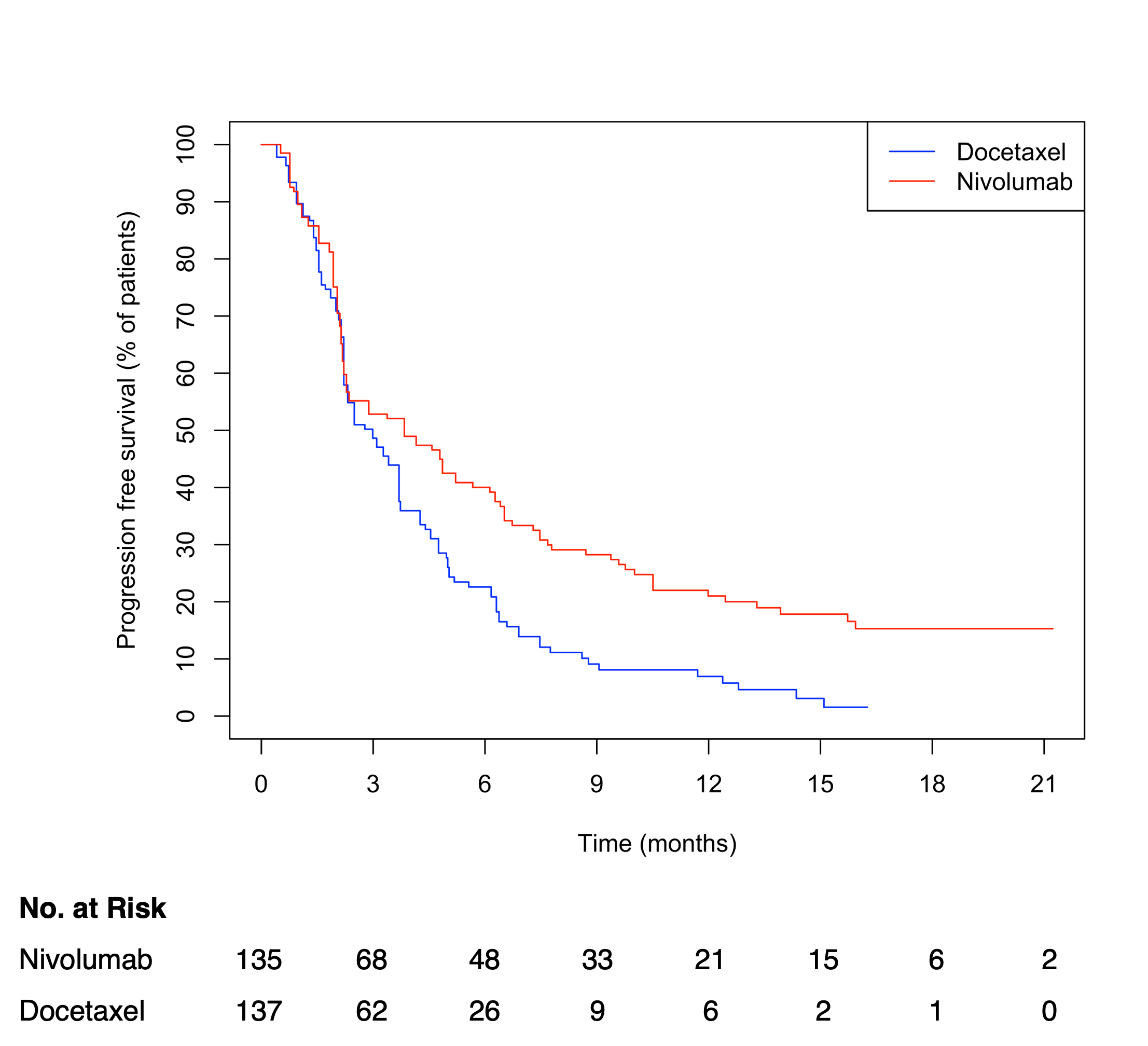
Figure 1: Kaplan-Meier plot of a Phase III trial, Checkmate 017¹², in which DTEs are present. The control and experimental treatment curves follow the same trajectory for approximately 3 months, after which they separate.

We introduce some notation. In a survival trial, suppose we have two groups: the control group and the experimental treatment group. We denote the hazard function for the control group as $h_{c}(t)$ and the hazard function for the experimental treatment group as $h_{c}(t)$.

In a typical survival trial, the alternative hypothesis, denoted as $H_{1}$, assumes that the hazard function for the experimental treatment group is less than or equal to the hazard function for the control group at all time points, that is $H_{1}$: $h_{t}(t)\leq h_{c}(t)$, $\forall t$. This suggests that patients in the experimental treatment arm immediately benefit from the intervention compared to those in the control arm. However, in a trial in which a DTE is thought likely to occur, we make a different assumption. We assume that the hazard function for the experimental treatment group is the same as that of the control group until a certain time $T$, which represents the delay in the experimental treatment taking effect. After time $T$, we assume that the experimental treatment group starts experiencing some benefit relative to the control group. Therefore, the hazard function for the experimental treatment group becomes a piecewise function:

$$h_{t}(t)=\begin{cases}h_{c}(t),&t\leq T\\ h^{*}_{t}(t),&t>T\end{cases},$$ (3)

where $h_{t}^{*}(t)\leq h_{c}(t)$ describes the benefit of the experimental treatment relative to control³¹.

In survival trials, the proportional hazards (PH) assumption is often made. This assumption states that the hazard ratio between the groups remains constant over time. It is used in Cox regression and the log-rank test, which is a standard statistical test in survival trials, is most powerful under this assumption. However, when DTEs are present, this assumption is violated because the hazard ratio becomes time-dependent. This poses challenges in designing and analyzing trials with DTEs.

Various researchers have proposed methodologies to address trials with DTEs^{33, 34, 35, 36, 37, 31, 38, 39, 40, 41}. However, most of these discussions focus on regaining statistical power lost due to the delay by using alternative analysis methods, such as weighted log-rank tests and the difference in restricted mean survival times (RMST)⁴². These methods aim to account for the time-dependent hazard ratio without assuming PH or the specific shape of the underlying survival curves.

3.2 Assurance for delayed treatment effects

As current literature focuses on power when DTEs are present, we introduce an elicitation technique and parameterisation to use in order to calculate assurance in these circumstances. By doing so, we are able to capture experts’ uncertainty of the relevant parameters and provide a more realistic judgement of the probability of success of the proposed trial. We suppose that the survival times in the control group follow a Weibull distribution with hazard function

$$h_{c}(t)=\gamma_{c}\lambda_{c}^{\gamma_{c}}t^{\gamma_{c}-1}$$ (4)

and corresponding survival function

$$S_{c}(t)=\text{exp}\{-(\lambda_{c}t)^{\gamma_{c}}\}.$$ (5)

We assume survival times in the experimental treatment group, after a delay of length $T$, also follow a Weibull distribution with different parameters to the control. This induces the hazard function

$$h_{t}^{*}(t)=\gamma_{t}\lambda_{t}^{\gamma_{t}}t^{\gamma_{t}-1}$$ (6)

and corresponding survival function

$$S_{t}^{*}(t)=\text{exp}\{-(\lambda_{c}T)^{\gamma_{c}}-\lambda_{t}^{\gamma_{t}}(t^{\gamma_{t}}-T^{\gamma_{t}})\}.$$ (7)

Prior to time $T$, we assume the experimental treatment group obeys the same survival function as the control (as seen in Equation 5). Thus, the survival function for the experimental treatment group is a piecewise function

$$S_{t}(t)=\begin{cases}\text{exp}\{-(\lambda_{c}t)^{\gamma_{c}}\},&t\leq T\\ \text{exp}\{-(\lambda_{c}T)^{\gamma_{c}}-\lambda_{t}^{\gamma_{t}}(t^{\gamma_{t}}-T^{\gamma_{t}})\},&t>T\end{cases}.$$ (8)

The hazard ratio of the two groups (derived from Equations 4 and 6) is

$$\text{HR}(t)=\begin{cases}1,&t\leq T\\ \frac{\gamma_{t}\lambda_{t}^{\gamma_{t}}t^{\gamma_{t}-1}}{\gamma_{c}\lambda_{c}^{\gamma_{c}}t^{\gamma_{c}-1}},&t>T\end{cases}.$$ (9)

3.3 Constructing the prior distributions

From Equations 5 and 8, we see that there are five unknowns: $T$, $\lambda_{c}$, $\gamma_{c}$, $\lambda_{t}$ and $\gamma_{t}$. To calculate assurance, prior distributions are required for these parameters. In the following sections we propose a method for eliciting these priors, including the questions to ask.

3.3.1 Prior for $T$

We first elicit judgements about $T$, the time at which the hazard function for the experimental treatment group differs from control and the treatment begins to take effect. We propose a prior of the form

$$T=\begin{cases}0,&\text{with probability }P_{\text{ND}}\\ D_{\text{delay}},&\text{with probability }1-P_{\text{ND}},\end{cases}$$ (10)

with $D_{\text{delay}}\sim\text{Gamma}(a,b)$. Any non-negative distribution could be used for $D_{\text{delay}}$ but we expect the Gamma distribution to be sufficiently flexible. We therefore need questions that an expert would be willing to answer and from which we can identify values for $P_{\text{ND}}$, $a$ and $b$. We elicit judgements about the probability $P_{\text{ND}}$ by asking the following question

“What is your probability that the treatment effect will not be subject to a delay? (i.e. the survival curves separate at time 0)”

We elicit judgements about the distribution of $D_{\text{delay}}$ by first stating

“Suppose that the treatment effect is subject to a delay. We now want you to consider your uncertainty about the delay.”

We would then use a standard method for eliciting a univariate distribution for $D_{\text{delay}}$. Methods for eliciting univariate distributions can be found in O’Hagan et al⁴³ and implemented using the Sheffield Elicitation Framework (SHELF)⁴⁴. SHELF is a package of protocols, templates and guidance documents for conducting expert elicitation. There are various methods that SHELF uses to elicit distributions, such as the ‘trial roulette’ method, or the ‘tertile’ and ‘quartile’ methods. In the ‘quartile’ method, the expert is asked to provide upper and lower bounds for the quantity of interest (QoI). They are also asked to provide values for the lower quartile, median, and upper quartile of the QoI. In all of the SHELF methods, parametric distributions are fit to these judgements using a least squares procedure: the parameters are chosen to ensure the fitted probabilities are as close as possible to elicited probabilities. Feedback is then provided to the expert to check the adequacy of the elicited distribution.

Example

Suppose the expert believes that there is a 10% chance that the treatment effect will not be subject to a delay and we set $P_{\text{ND}}$ = 0.1. To elicit beliefs about the distribution $D_{\text{delay}}$, we use the quartile method as described above. If the expert provides a lower quartile of 4, a median of 6 and an upper quartile of 8 then a Gamma($a,b$) distribution which captures these judgements sufficiently well is a Gamma(4.09, 0.642) distribution. Combining these beliefs, we obtain the following mixture prior distribution for $T$:

$$T=\begin{cases}0,&\text{with probability }0.1\\ \text{Gamma}(4.09,0.642),&\text{with probability }0.9.\end{cases}$$

The fitted quartiles of a Gamma(4.09, 0.642) distribution are 4.07, 5.87 and 8.13. In an elicitation session, the expert would be presented with this distribution and additional quantities, with the opportunity to revise judgements and change the distribution as appropriate.

3.3.2 Prior(s) for $\lambda_{c}$, $\gamma_{c}$

There are two parameters to elicit judgements on for the survival times in the control group; $\lambda_{c}$, also known as the scale parameter, and $\gamma_{c}$, the shape parameter. We assume that there exists some historical data about the intervention that will be used in the control group, that is

$$\pi(\lambda_{c},\gamma_{c}|\boldsymbol{x}_{\text{hist}}),$$

where $\boldsymbol{x}_{\text{hist}}$ is the historical data for the control group intervention. We assume we are able to use this historical data to specify prior distributions for the parameters. Schmidli et al⁴⁵ consider using a meta-analytic-predictive (MAP) prior for parameters in the control group when there are historical data available. Bertsche et al⁴⁶ extend this method to specifically consider time-to-event data. Alternatively, to include expert elicitation at this stage, see Ren and Oakley²¹, who consider eliciting beliefs when survival times are assumed to follow a Weibull distribution (among other distributions).

3.3.3 Prior(s) for $\lambda_{t}$, $\gamma_{t}$

The final two parameters which we need to elicit beliefs on are the two treatment parameters, $\lambda_{t}$ and $\gamma_{t}$. We would not expect an expert to make judgements about these parameters directly. We instead follow usual elicitation practice of eliciting judgments about observable quantities⁴⁷, from which a prior for $\lambda_{t}$, $\gamma_{t}$ can be inferred. Possible choices of observable quantities are

• median survival time on the experimental treatment;

• survival probability at time $t$; and

• greatest distance between survival curves and how big is this difference.

In practice, we have found experts have a preference to make judgements about hazard ratios, e.g.

• hazard ratio at time $t$; and

• maximum hazard ratio and when this occurs.

To elicit both parameters, $\lambda_{t}$ and $\gamma_{t}$, we require the expert to provide their beliefs for at least two of the above questions. However, if we make a simplifying assumption that $\gamma_{t}=\gamma_{c}$ then Equation 9 reduces to

$$\text{HR}(t)=\begin{cases}1,&t\leq T\\ \bigg{(}\frac{\lambda_{t}}{\lambda_{c}}\bigg{)}^{\gamma_{c}},&t>T\end{cases}.$$ (11)

We can rearrange Equation 11, for the case when $t>T$, to obtain

$$\lambda_{t}=\lambda_{c}\text{HR}^{\frac{1}{\gamma_{c}}}.$$ (12)

In Equation 12, we have two known parameters, $\lambda_{c}$ and $\gamma_{c}$, and two unknown parameters, $\lambda_{t}$ and HR. Therefore, we are able to indirectly elicit beliefs about $\lambda_{t}$ by asking questions about the hazard ratio (HR) for when $t>T$ (known as the post-delay hazard ratio, $\text{HR}^{*}$, from now on). As such, we believe that this quantify is a sensible one to ask about and one that the experts will be happy to answer. Hence the assumption $\gamma_{t}=\gamma_{c}$ simplifies the elicitation task. We investigate the implications of this assumption in Section 6.

For $\text{HR}^{*}$, we propose a prior of the form

$$\text{HR}^{*}=\begin{cases}1,&\text{with probability }P_{\text{NE}}\\ D_{\text{HR}},&\text{with probability }1-P_{\text{NE}},\end{cases}$$ (13)

with $D_{\text{HR}}\sim\text{Gamma}(c,d)$. Again, any non-negative distribution could be used for $D_{\text{HR}}$. As with $T$, we therefore need questions that an expert would be willing to answer and from which we can identify values for $P_{\text{NE}}$, $c$ and $d$. We elicit judgements about the probability $P_{\text{NE}}$ by asking the following

“What is your probability that the experimental treatment will not show some benefit compared to the control?”

We elicit judgements about the distribution $D_{\text{HR}}$ by stating

“Suppose that the experimental treatment will show some efficacy compared to control. We now want you to consider your uncertainty about the hazard ratio once the experimental treatment begins to take effect.”

We would then use a standard method for eliciting a univariate distribution for $D_{\text{HR}}$, as presented in Section 3.3.1.

Example

Suppose the expert believes that there is a 5% chance that the experimental treatment will not show any benefit compared to control, then $P_{\text{NE}}=0.05$. For the distribution $D_{\text{HR}}$, using the quartile method: if the expert provides a lower quartile of 0.4, a median of 0.55 and an upper quartile of 0.65, then a Gamma(7.8, 14.1) sufficiently captures these beliefs. Combining these results, we obtain the following mixture prior for the post-delay hazard ratio:

$$\text{HR}^{*}=\begin{cases}1,&\text{with probability }0.05\\ \text{Gamma}(7.8,14.1),&\text{with probability }0.95,\end{cases}$$

The fitted quartiles of the Gamma(7.8, 14.1) distribution are 0.41, 0.53 and 0.67. As before, the distribution would be presented to the expert for feedback.

3.4 Computing assurance under the DTE model

We can use these mixture priors to calculate the assurance of a trial for different sample sizes using Algorithm 1. There are a number of free parameters ($n_{c},n_{t}$ and $E$) in Algorithm 1 that can be changed to reflect the operational constraints that might be present when running a clinical trial. Changing these parameters will have consequences on the assurance calculated, so it is important to consider different combinations of trial designs, to find the one which best suits the needs of the sponsor. For example, for a fixed $n_{c}$ and $n_{t}$, if we increase $E$ (the number of events) then we will almost surely increase the assurance, but this will come at the cost of needing to run the trial for a longer time.

In principle, it is easy to extend Algorithm 1 (and Algorithm 2, presented in Section 6.2) to suit the needs of the proposed clinical trial. For example, in both algorithms, a log-rank test is the method of analysis. However, any other choice of analysis— for example, a weighted log-rank test or difference in RMST curves—can be substituted into this stage of the algorithm, and the algorithm remains valid, as long as this analysis method is the one that would be implemented in practice. More complex trial designs can also be accommodated, such as more sophisticated recruitment schedules (compared to the default uniform recruitment, between time 0 and $R$) and to include interim analyses (or any other form of group sequential design).

Algorithm 1 calculating assurance when a DTE is present in a clinical trial

Inputs: sample sizes $n_{c}$ and $n_{t}$, the control prior $\pi(\lambda_{c},\gamma_{c})$, the elicited mixture priors $\pi(T)\pi(\text{HR}^{*})$, the number of events $E$ (we require $E\leq n_{c}+n_{t}$), the recruitment length $R$ and the number of iterations $N$.
For $i=1,\ldots,N$:

1. sample $\lambda_{c,i},\gamma_{c,i}$ from $\pi(\lambda_{c},\gamma_{c})$;

2. sample survival times for the control group $x_{1,i},\ldots,x_{n_{c},i}$ using $\lambda_{c,i}$, $\gamma_{c,i}$ (can use rweibull());

3. sample $T_{i},\text{HR}^{*}_{i}$ from $\pi(T)\pi(\text{HR}^{*})$;

4. transform $\text{HR}^{*}$ to $\lambda_{t,i}$ using Equation 12;

5. set $\gamma_{t,i}=\gamma_{c}$;

6. sample survival times for the experimental treatment group $y_{1,i},\ldots,y_{n_{t},i}$ using $T_{i}$, $\lambda_{t,i}$ and $\gamma_{t,i}$ (can use inversion sampling via Equation 8);

7. sample recruitment times $R_{1,i},\ldots,R_{n_{c}+n_{t},i}$ from Unif(0, $R$);

8. add the survival times from each group to the recruitment times to obtain a pseudo event time $P_{1,i},\ldots,P_{n_{c}+n_{t},i}$;

9. order the pseudo event times and define $E_{T}$ to be the time at which $E$ events have been observed;

10. remove any observation in which the recruitment time $R_{j,i}$ > $E_{T}$;

11. censor any observation for which the pseudo event time $P_{j,i}$ > $E_{T}$;

12. for any censored observation, redefine the survival time to be $E_{T}-R_{j,i}$;

13. perform the log-rank test and obtain the test statistic $S_{i}$ from $x_{1,i},\ldots,x_{n_{c},i}$ and $y_{1,i},\ldots,y_{n_{t},i}$;

14. define $U_{i}=1$ if $S_{i}$ > $\chi_{1,\alpha}^{2}$ and 0 otherwise, with $\chi_{1,\alpha}^{2}$ the $(100-\alpha)$th percentile of the Chi-squared distribution with 1 degree of freedom.

The assurance is then estimated as

$$\hat{P}(R)=\frac{1}{N}\sum^{N}_{i=1}U_{i}.$$

4 Software

We have developed open-source software — in the form of an R package and an online R Shiny app — for implementing the methodology introduced in Section 3. Instructions for downloading this software are found in the Appendix. Figures 3 and 4 are screenshots from the Shiny App, they are taken from the example given in Section 5.

5 Example

In this section, we illustrate the methods presented for calculating assurance for when a DTE is likely to be present in a trial. In this (hypothetical) example, we assume we are designing a two-arm Phase III superiority trial to test whether a new drug is beneficial versus the current standard of care, docetaxel, in patients with advanced non–small-cell lung cancer (NSCLC). As the drug is in the IO area, we are expecting a DTE to be present in the trial. The primary efficacy endpoint is overall survival, we assume uniform recruitment for 6 months, 1:1 allocation, and the data will be analysed with a log-rank test. We assume that the trial will be analysed (and the remaining patients censored) at an information fraction of 80%, that is when 80% of the prespecified sample size have experienced the event.

5.1 Prior distribution(s) for the control parameters

There exists historical data about the intervention that will be used in the control group, docetaxel, so we are able to use this prior knowledge to generate a distribution for the control group. In Bertsche et al⁴⁶, they found three trials in which docetaxel was used as the control in a clinical trial; INTEREST⁴⁸, ZODIAC⁴⁹ and REVEL⁵⁰. We also use the results from these three trials, but we use the published Kaplan-Meier curves to reconstruct the individual patient data³⁰. The three Kaplan-Meier curves can be see in in Figure 2. From the Kaplan-Meier curves, we see that all three of the trials seem fairly exchangeable, so we choose to pool the data from all three trials together. We then generate a posterior Monte Carlo Markov Chain (MCMC) sample for the two Weibull parameters, $\lambda_{c}$ and $\gamma_{c}$, using non-informative priors. The generated MCMC sample is then used as a prior distribution for the future trial of interest.

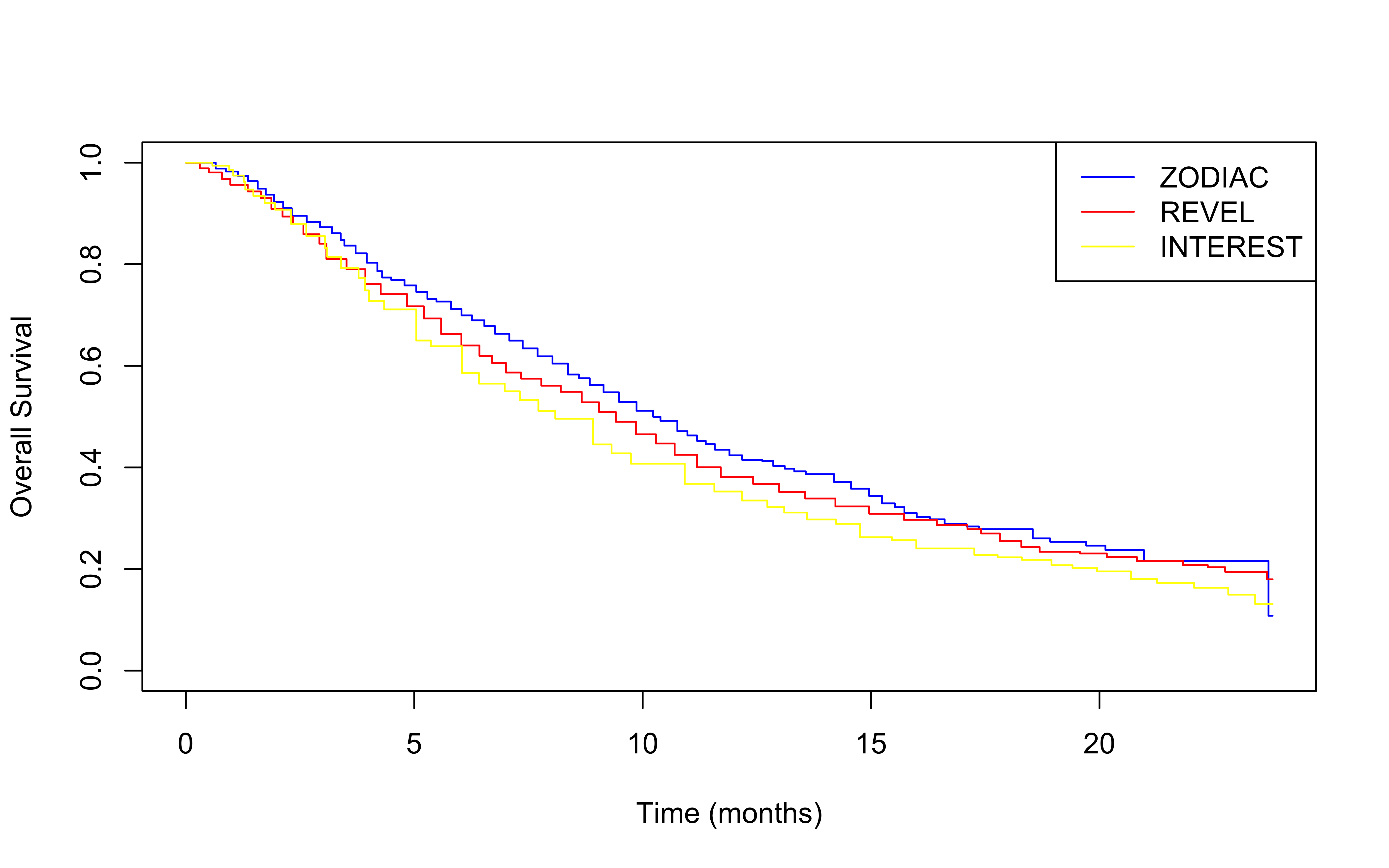
Figure 2: Reconstructed Kaplan-Meier curves for the docetaxel arm in three different trials: ZODIAC⁴⁹, REVEL⁵⁰ and INTEREST⁴⁸. We see that the three curves are similar and we assume exchangeability of the trials in our example.

5.2 Eliciting the prior distribution for the length of delay

The first QoI we elicit is the time at which the experimental treatment begins to take effect, relative to the control. We suppose that the expert believes that the probability that the experimental treatment will not be subject to a delay is 5%, that is $P_{\text{ND}}$ = 0.05. The expert is then asked about their beliefs about the length of the delay, conditional on there being a delay. The expert provides a median of 4 and two quartiles (25% and 75%) of 3 and 5, respectively. A Gamma($a,b$) distribution is fitted to these judgements, so $D_{\text{delay}}$ = Gamma(7.29, 1.76). Combining these beliefs using Equation 10, we have the following mixture prior distribution

$$T=\begin{cases}0,&\text{with probability }0.05\\ \text{Gamma(7.29, 1.76)},&\text{with probability }0.95\end{cases}.$$

The fitted quartiles of a Gamma(7.29, 1.76) distribution are 3.03, 3.95 and 5.05. The process of fitting this distribution is seen in Figure 3, which is a screenshot from the DTEAssurance Shiny App.

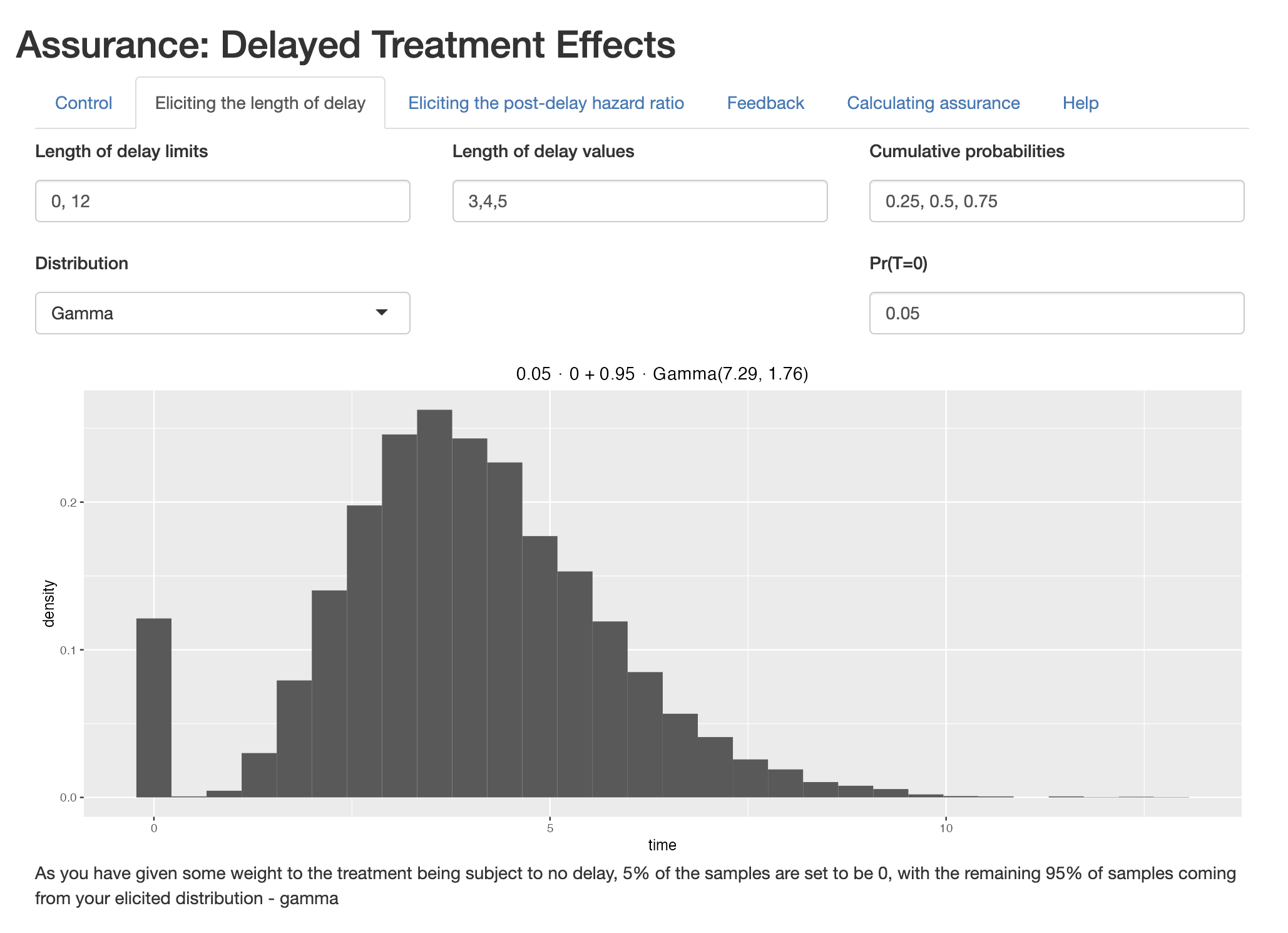
Figure 3: Screenshot from the DTEAssurance Shiny App (see Appendix). This tab shows elicitation of the length of delay, $T$, using the SHELF⁴⁴ ‘quantile’ method, as described in 3.3.1. The values used are the same as the example elicitation, seen in Section 5.2.

5.3 Eliciting the prior distribution for the post-delay hazard ratio

The second QoI is the hazard ratio exhibited once the experimental treatment begins to take effect, $\text{HR}^{*}$. We suppose that the expert believes that the probability that the experimental treatment will work no better than the control is 10%, that is $P_{\text{NE}}$ = 0.1. We then ask the expert to consider the case that the experimental treatment is better than the control and elicit their beliefs about the post-delay hazard ratio. The expert provides a median of 0.6 and two quartiles (25% and 75%) of 0.55 and 0.7, respectively. Again, we fit a Gamma($c,d$) to these judgements, so $D_{\text{HR}}$ = Gamma(29.6, 47.8). Again, combining these beliefs using Equation 13, we have the following mixture prior distribution

$$\text{HR}^{*}=\begin{cases}1,&\text{with probability }0.1\\ \text{Gamma(29.6, 47.8)},&\text{with probability }0.9\end{cases}.$$

The fitted quartiles of aGamma(29.6, 47.8) distribution are 0.54, 0.61 and 0.69.

5.4 Calculating assurance

We use these elicited prior distributions to calculate assurance for this example using Algorithm 1. Figure 4 is a screenshot from the DTEAssurance Shiny App, showing the calculated assurance curve given the elicited distributions. Furthermore, in Figure 5, an assurance curve is plotted to inform sample sizes required for this clinical trial. Also seen in Figure 5 are three other power/assurance curves. The two power curves correspond to including no uncertainty in the parameters, with the control parameters, $\lambda_{c}$ and $\gamma_{c}$, being the MLE from the three pooled data sets, as discussed in Section 5.1. The values for $T$ and $\text{HR}^{*}$ are the median values given by the experts. For one of the power curves, we have assumed that $T$ is 0, and therefore does not account for the fact that the treatment effect may be subject to a delay. Also shown is an assurance curve, corresponding to a more flexible approach to calculating assurance, this approach is presented in Section 6.2. The distributions/values for the first three curves are found in Table 1. We kept the recruitment scheduling, analysis method etc, as described at the start of Section 5, constant across all four scenarios.

In Figure 5, we see that both of the power calculations are much more optimistic than the other two scenarios; we require far fewer patients for the same power, at all sample sizes. This highlights the importance of incorporating uncertainty into the trial parameters. However, we must reiterate, the assurance method is not simply used for setting sample sizes for the proposed trial. We anticipate the assurance method being used as one step in a thorough process to decide whether or not to go ahead with the trial, and if we do run the trial, define the characteristics of the proposed trial; length, number of patients, number of events etc. For example, if we required a quicker trial, we may choose to decrease the number of events we need to observe before stopping the trial, $E$, but this will surely come at a cost of reducing the assurance/power seen. Therefore, it is important that a number of different trial designs are considered, and then assurance curves can be plotted to help inform the ultimate decision(s).

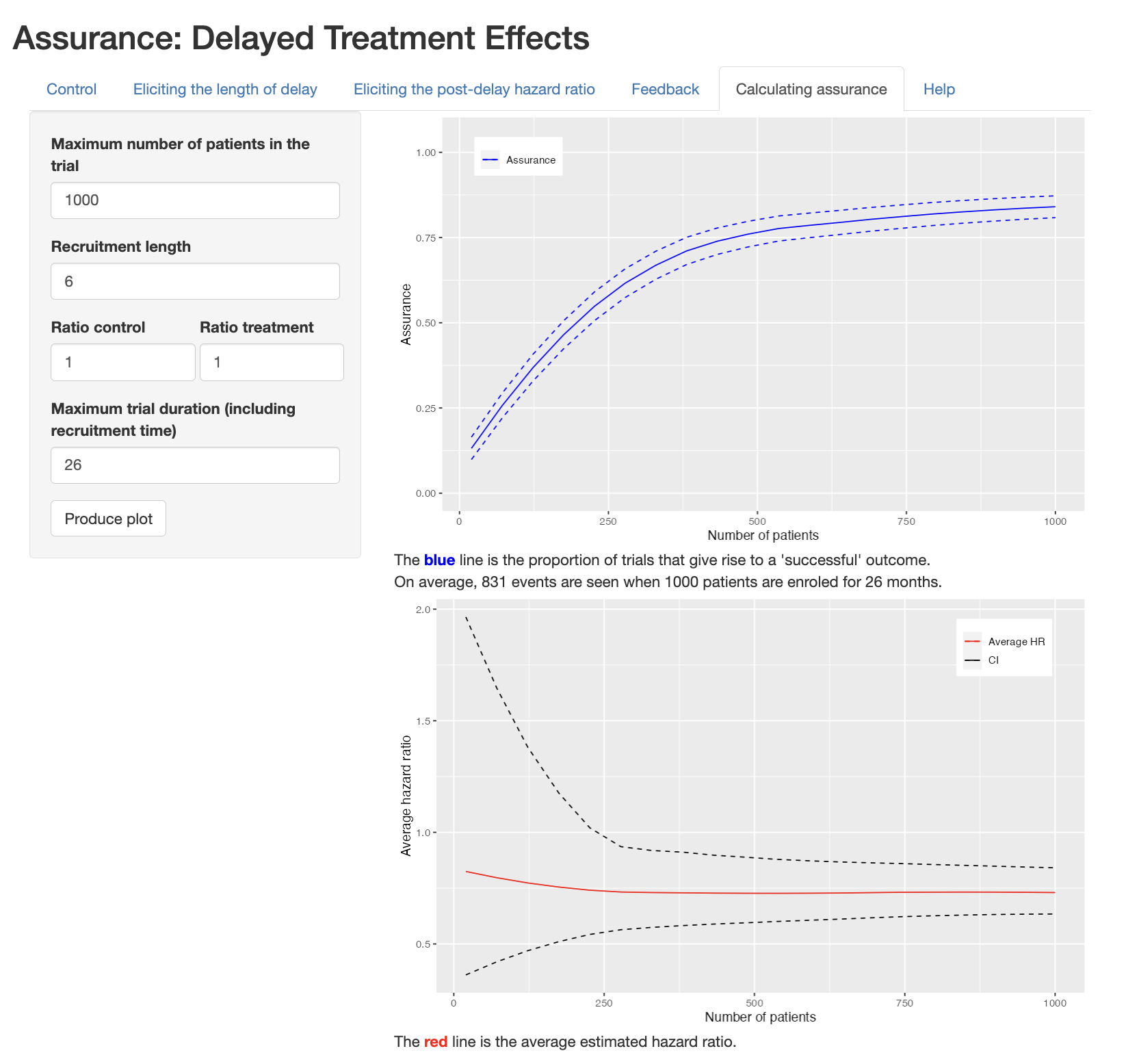
Figure 4: Screenshot from the DTEAssurance Shiny App (see Appendix). This tab shows the calculated assurance, given the input from the previous tabs (not shown) and the questions regarding the trial operating characteristics seen on the left-hand side. The inputs are the same as the example given in Section 5, and as such, the assurance curve is similar to the assurance curve seen in Figure 5.

Calculation	$\lambda_{c}$	$\gamma_{c}$	T	post-delay HR
Assurance	MCMC sample	MCMC sample	$\begin{cases}0,&\text{w.p. }0.05\\ \text{Ga}(7.29,1.76),&\text{w.p. }0.95\end{cases}$	$\begin{cases}0,&\text{w.p. }0.1\\ \text{Ga}(29.6,47.8),&\text{w.p. }0.9\end{cases}$
Power	1.21	0.074	4	0.6
Power assuming no delay	1.21	0.074	0	0.6

Table 1: Distribution/values for the parameters, for the first three scenarios seen in Figure 5.

Figure 5: Power/assurance curves for the example given in Section 5. We see that the sample size required for 80% power/assurance is greatly different under the different scenarios and highlights the importance of including uncertainty in the design stage of a clinical trial

6 Simplified prior distribution: discussion

To elicit the parameters in this scenario, we had to make a decision on the method that would be both effective and straightforward for the experts. As a result, we simplified the original parameterisation by fixing $\gamma_{t}=\gamma_{c}$. By doing so, we were able to focus on hazard ratios as the basis for our questioning, thus ensuring that the elicitation process was both easy and intuitive for the experts.

However, it’s important to investigate the robustness of this simplification. The results of our investigation are presented in the following section. Finally, we provide an alternative method for calculating assurance. This alternative is designed to accommodate situations in which the aforementioned simplification may not be preferred.

6.1 Robustness of the parameterisation

The investigation aimed to assess the impact of the simplification we introduced, $\gamma_{t}=\gamma_{c}$, into the model by comparing two parameterisation methods: Method A and Method B. Method A incorporated the simplification, while Method B allowed $\gamma_{t}$ to vary. Historical data from three clinical trials (Checkmate 017¹², Checkmate 141⁵¹, and Checkmate 017 and Checkmate 057 combined⁵², the Kaplan-Meier plots for these trials are seen in Figure 6) with observed DTE were used to estimate the five unknown parameters using both methods. For each of the three trials, we estimated the five unknown parameters in the parameterisation (from Equations 5 and 8) using the two methods introduced above. For clarity, Table 2 shows how the two methods estimate the five unknown parameters.

Figure 6: Kaplan-Meier plots for the data sets introduced in Section 6. For (a) the data set is from trial Checkmate 017¹², for (b) the data set is from trial Checkmate 141⁵¹ and for (c) the data set is from trials Checkmate 017 and Checkmate 057 combined⁵².

The estimated parametric survival curves generated by both methods are presented in Figure 7. Observing all three examples, we can see that the parametric treatment survival curve produced by Method B exhibits a marginally superior fit compared to the treatment curves derived from Method A. This is what we would intuitively expect, as Method B incorporates two free parameters, $\gamma_{t}$ and $\gamma_{c}$, while Method A only employs a single free parameter, $\gamma_{c}$. However, despite Method B giving a better fit to the data, Method A still approximates the data well. These findings suggest that even with the simplification introduced by Method A, the simplification introduced would likely have minimal practical impact on real decision-making processes.

Figure 7: The same Kaplan-Meier plots as in Figure 6, with estimates for both Method A and B (as introduced in Section 6) overlaid. For each data set, $T$ has been visually estimated. The control parameters, $\lambda_{c}$ and $\gamma_{c}$, have been estimated from the data (the overlaid blue line). In Method A, the simplification has been made ($\gamma_{t}=\gamma_{c})$ and then $\lambda_{t}$ has been estimated using a least squares procedure. In Method B, both the treatment parameters ($\lambda_{t},\gamma_{t})$ have been simultaneously estimated.

Power calculations were performed to quantify the difference in the experimental treatment survival curves. The results, depicted in Figure 8, showed almost indistinguishable power curves for both methods across all three datasets. This suggests that, in these examples, the assumption $\gamma_{t}=\gamma_{c}$ did not lead to different practical outcomes.

Method	$\boldsymbol{T}$	$\boldsymbol{\gamma_{c}}$	$\boldsymbol{\lambda_{c}}$	$\boldsymbol{\gamma}_{t}$	$\boldsymbol{\lambda}_{t}$
A	Visually	survreg(dist = "weibull")		$\gamma_{c}$	MLE
B				MLE	MLE

Table 2: How each of the five parameters are estimated in both of the methods introduced in Section 6, Method A is the simplification we made in the elicitation process (MLE = Maximum Likelihood Estimation).

Figure 8: Power curves for the two methods considered in Section 6, for all three of the trials. We see that, in all three cases, the power curves are very similar to each other, thus indicating that the simplification does not seem make any practical difference in these examples. Method A is the simplification we made in the elicitation process.

6.2 A more flexible approach to evaluating assurance

We have demonstrated that for the three historical trials considered, the simplification does not appear to have any practical implications. However, by making this simplification, the possible experimental treatment survival curves are constrained to align with the shape of the control survival curve. In Figure 9(a), it can be observed that the experimental treatment survival curves seem to be ‘parallel’ to the control curve due to this simplification and the fixed shape parameters, $\gamma_{t}=\gamma_{c}$, being the same for both curves.

Figure 9: (a) 10 sampled experimental treatment survival curves, generated by Algorithm 1, (b) pointwise confidence intervals (0.1 and 0.9) for 500 of these sampled experimental treatment curves, (c) 10 sampled experimental treatment survival curves, generated by Algorithm 2, (d) pointwise confidence intervals (0.1 and 0.9) for 500 of these sampled experimental treatment curves.

It is important to acknowledge that in certain trial designs, practitioners may feel uneasy about using this method, particularly if they believe that the experimental treatment survival curve would not align in a parallel manner to the control curve. In response to this concern, we have developed an alternative assurance calculation, referred to as Algorithm 2. Algorithm 2 aims to generate experimental treatment curves that would be obtained if we had not made the simplification and allowed the curves to be sampled from a Weibull($\lambda_{t},\gamma_{t}$) distribution after the delay occurred. The process is depicted in Figure 10.

To implement Algorithm 2, we utilize the elicited mixture prior distributions for $T$ and $\text{HR}^{*}$. First, we sample a large number of experimental treatment curves, denoted as $M$. Next, we sample a value for $T$ from the elicited prior distribution, as shown in Figure 10(a). We define $F$ as the time at which the control curve reaches a survival probability of 0.01. Then, we independently sample two survival probabilities, $s_{1}$ and $s_{2}$, at 0.25$F$ and 0.6$F$ through the trial, respectively, as depicted in Figure 10(b) and 10(c). The only condition imposed is that $s_{1}>s_{2}$. Using $T$, $s_{1}$ and $s_{2}$, we apply a least squares procedure to fit a Weibull distribution to these points, as illustrated in Figure 10(d).

The sampled experimental treatment curves obtained from Algorithm 2 can be used to calculate assurance in the same manner as Algorithm 1. Figure 9(c) displays 10 sampled experimental treatment curves using this more flexible method. Additionally, Figure 9(d) shows the pointwise confidence intervals of the experimental treatment curves. Comparing these figures to Figures 9(a) and (b), we observe that the pointwise confidence intervals are very similar, indicating that the sampled experimental treatment curves fall within the same boundaries. However, the alternative method allows for sampling a more diverse range of curves, providing increased flexibility.

We have implemented Algorithm 2 in the example presented in Section 5, and the results are seen in Figure 1. The flexible assurance curve closely resembles the assurance curve obtained using Algorithm 1. This demonstrates that the more flexible assurance method may not significantly impact decision-making, but it may make practitioners more comfortable if they believe that the imposed constraint is not representative of the potential experimental treatment curves observed in practice. It is worth noting that the selection of time points (0.25$F$ and 0.6$F$) for sampling survival probabilities in Algorithm 2 is somewhat arbitrary. These values were chosen to produce realistic experimental treatment survival curves. However, if more restrictive or flexible curves are desired, these two points could be adjusted accordingly (e.g., closer together or further apart).

Figure 10: Showing the process of how an experimental treatment survival line is drawn for the flexible assurance. (a) a delay time is drawn from the prior distribution for $T$, (b) $s_{1}$ is sampled from all the survival probabilities at $0.25F$ through the trial, (c) $s_{2}$ is sampled from all the survival probabilities at $0.6F$ through the trial, (d) a piecewise Weibull distribution is fit to these sampled points.

Algorithm 2 calculating flexible assurance for when DTEs are present

Inputs: sample sizes $n_{c}$ and $n_{t}$, the control prior $\pi(\lambda_{c},\gamma_{c})$, the elicited mixture prior $\pi(T,\text{HR}^{*})$, the number of events $E$ (we require $E\leq n_{c}+n_{t}$), the maximum trial length $L_{\text{max}}$, the recruitment length $R$, the number of initial samples $M$ and the number of iterations $N$.

1. Initialise an empty matrix $S\in\mathbb{R}^{M\times t}$, where $t$ is the length of a vector time = seq(0, $L_{\text{max}}$, by = 0.01);

2. for $j=1,\ldots,M$:

   1. sample $\lambda_{c,j},\gamma_{c,j}$ from $\pi(\lambda_{c},\gamma_{c})$;

   2. sample $T_{j}$, $\text{HR}^{*}_{j}$ from $\pi(T,\text{HR}^{*})$;

   3. transform $\text{HR}^{*}_{j}$ to $\lambda_{t,j}$ using Equation 12;

   4. set $\gamma_{t,j}=\gamma_{c}$;

   5. use $T_{j}$, $\lambda_{t,j}$, $\gamma_{t,j}$, and the control parameters $\lambda_{c}$, $\gamma_{c}$ to calculate the survival probability at each value of the time vector, using Equation 8;

   6. fill the $j$’th row of the matrix $S$ with these survival probabilities.

3. For $i=1,\ldots,N$:

   1. sample $\lambda_{c,i},\gamma_{c,i}$ from $\pi(\lambda_{c},\gamma_{c})$;

   2. define $F$ to be the time at which the survival probability in the control group equals 0.01 (using $\lambda_{c,i},\gamma_{c,i}$ and Equation 5);

   3. sample a survival probability, $s_{1,i}$, from the column in matrix $S$ which corresponds to $0.25F$;

   4. sample a survival probability, $s_{2,i}$ from the column in matrix $S$ which corresponds to $0.6F$ (we require $s_{2,i}<s_{1,i}$);

   5. sample $T_{i}$ from $\pi(T)$;

   6. simultaneously solve these equations to find the best fitting values of $\lambda_{t,i}$ and $\gamma_{t,i}$ (can use nleqslv());

   7. sample survival times for the control group $x_{1,i},\ldots,x_{n_{c},i}$ using the sampled $\lambda_{c,i}$, $\gamma_{c,i}$ (can use rweibull());

   8. sample survival times for the experimental treatment group $y_{1,i},\ldots,y_{n_{t},i}$ using the sampled $T_{i}$, and $\lambda_{t,i}$, $\gamma_{t,i}$ (can use inversion sampling);

   9. sample recruitment times $R_{1,i},\ldots,R_{n_{c}+n_{t},i}$ from Unif(0, $R$);

   10. add the survival times from each group to the recruitment times to obtain a pseudo event time $P_{1,i},\ldots,P_{n_{c}+n_{t},i}$;

   11. order the pseudo event times and define $E_{T}$ to be the time at which $E$ events have been observed;

   12. remove any observation in which the recruitment time $R_{j,i}$ > $E_{T}$;

   13. censor any observation for which the pseudo event time $P_{j,i}$ > $E_{T}$;

   14. for any censored observation, redefine the survival time to be $E_{T}-R_{j,i}$;

   15. perform the log-rank test and obtain the test statistic $S_{i}$ from $x_{1,i},\ldots,x_{n_{c},i}$ and $y_{1,i},\ldots,y_{n_{t},i}$;

   16. define $U_{i}=1$ if $S_{i}$ > $\chi_{1,\alpha}^{2}$ and 0 otherwise, with $\chi_{1,\alpha}^{2}$ the $(100-\alpha)$th percentile of the Chi-squared distribution with 1 degree of freedom.

The assurance is then estimated as

$$\hat{P}(R)=\frac{1}{N}\sum^{N}_{i=1}U_{i}.$$

7 Summary

In conclusion, assurance calculations have emerged as a valuable tool in the design and analysis of clinical trials. By incorporating Bayesian principles and considering prior distributions for unknown parameters, assurance calculations provide a more realistic assessment of a trial’s probability of success compared to traditional power calculations. This approach acknowledges the inherent uncertainties in clinical research and allows for the simulation of trial outcomes based on sampled prior distributions.

Assurance calculations offer several advantages for trial design and decision-making. They assist in optimizing sample size, assessing risks, and evaluating the effectiveness of different trial setups, including the timing and number of planned interim analyses. Furthermore, assurance evaluations enable better-informed go/no-go decisions regarding study conduct, directing resources towards research programs with the highest expected impact for patients.

In the rapidly evolving field of immuno-oncology, assurance calculations have the potential to address challenges associated with non-constant treatment effects and delayed treatment effects on time-to-event endpoints. We have extended the assurance method to include survival trials in which a delayed treatment effect is likely to occur.

Overall, assurance calculations provide a robust framework for quantifying the probability of success in clinical trials while considering uncertainty. By incorporating Bayesian methods and accommodating complexities in trial design, assurance calculations contribute to more informed decision-making, improved trial design, and ultimately, more effective and impactful clinical research.

ACKNOWLEDGEMENTS

This work has been supported by a University of Sheffield EPSRC Doctoral Training Partnership (DTP) Case Conversion with Novartis Scholarship [project reference 2610753].

DATA AVAILABILITY STATEMENT

Data sharing is not applicable to this article, as no new data were created or analysed in this study.

An R⁵³ package, DTEAssurance, for implementing the methods described in this paper is available on GitHub, at https://github.com/jamesalsbury/DTEAssurance. The website also includes an illustration of using the package to replicate the examples in this paper. This package is installed with the commands

install.packages("devtools")

devtools::install_github("jamesalsbury/DTEAssurance").

An app for implementing these methods, produced with shiny⁵⁴, can be used online at https://jamesalsbury.shinyapps.io/DTEApp/. A version of the app for offline use is included in the DTEAssurance package.

References

- 1 Spiegelhalter DJ, Freedman LS. A predictive approach to selecting the size of a clinical trial, based on subjective clinical opinion. Stat Med. 1986;5(1):1-13. doi:10.1002/sim.4780050103
- 2 O’Hagan A, Stevens JW, Campbell MJ. Assurance in clinical trial design. Pharmaceutical Statistics 2005;4. 187 - 201. doi:10.1002/pst.175.
- 3 Grieve, A.P. (2022). Hybrid Frequentist/Bayesian Power and Bayesian Power in Planning Clinical Trials (1st ed.). Chapman and Hall/CRC. https://doi.org/10.1201/9781003218531
- 4 Crisp A, Miller S, Thompson D, Best N. Practical experiences of adopting assurance as a quantitative framework to support decision making in drug development. Pharm Stat. 2018;17(4):317-328. doi:10.1002/pst.1856
- 5 Kinnersley N, Day S. Structured approach to the elicitation of expert beliefs for a Bayesian-designed clinical trial: a case study. Pharm Stat. 2013;12(2):104-113. doi:10.1002/pst.1552
- 6 Hampson LV, Holzhauer B, Bornkamp B, et al. A New Comprehensive Approach to Assess the Probability of Success of Development Programs Before Pivotal Trials. Clin Pharmacol Ther. 2022;111(5):1050-1060. doi:10.1002/cpt.2488
- 7 Hampson LV, Bornkamp B, Holzhauer B, et al. Improving the assessment of the probability of success in late stage drug development. Pharmaceutical Statistics. 2022; 21( 2): 439- 459. doi:10.1002/pst.2179
- 8 Götte, H., Schüler, A., Kirchner, M., and Kieser, M. (2015) Sample size planning for phase II trials based on success probabilities for phase III. Pharmaceut. Statist., 14: 515– 524. doi: 10.1002/pst.1717.
- 9 US Food and Drug Administration . 22 Case Studies Where Phase 2 and Phase 3 Trials Had Divergent Results. FDA 2017.
- 10 Dallow N, Best N, Montague TH. Better decision making in drug development through adoption of formal prior elicitation. Pharm Stat. 2018;17(4):301-316. doi:10.1002/pst.1854
- 11 Jiménez JL, Stalbovskaya V, Jones B. Properties of the weighted log-rank test in the design of confirmatory studies with delayed effects. Pharmaceutical Statistics. 2019; 18, 287 - 303.
- 12 Brahmer J, Reckamp KL, Baas P, et al. Nivolumab versus Docetaxel in Advanced Squamous-Cell Non-Small-Cell Lung Cancer. N Engl J Med. 2015;373(2):123-135. doi:10.1056/NEJMoa1504627
- 13 Mukhopadhyay P, Ye J, Anderson KM, et al. Log-Rank Test vs MaxCombo and Difference in Restricted Mean Survival Time Tests for Comparing Survival Under Nonproportional Hazards in Immuno-oncology Trials: A Systematic Review and Meta-analysis. JAMA Oncol. 2022;8(9):1294–1300. doi:10.1001/jamaoncol.2022.2666
- 14 Rizvi NA, Cho BC, Reinmuth N, et al; MYSTIC Investigators. Durvalumab with or without tremelimumab vs standard chemotherapy in first-line treatment of metastatic non-small cell lung cancer: the MYSTIC phase 3 randomized clinical trial. JAMA Oncol. 2020;6(5):661-674. doi:10.1001/jamaoncol.2020.0237
- 15 Herbst RS, Giaccone G, de Marinis F, et al; MYSTIC Investigators. Atezolizumab for First-Line Treatment of PD-L1-Selected Patients with NSCLC. N Engl J Med. 2020;383(14):1328-1339. doi:10.1056/NEJMoa1917346
- 16 Shitara K, Van Custem E, Bang YJ, et al. Efficacy and safety of pembrolizumab or pembrolizumab plus chemotherapy vs chemotherapy alone for patients with first-line, advanced gastric cancer: the KEYNOTE-062 phase 3 randomized clinical trial. JAMA Oncol. 2020;6(10):1571-1580. doi:10.1001/jamaoncol.2020.3370
- 17 International Council for Harmonisation. Addendum on estimands and sensitivity analysis in clinical trials to the guideline om statistical principles for clinical trials E9(R) (https://database.ich.org/sites/default/files/E9-R1_Step4_Guideline_2019_1203.pdf). 2019.
- 18 Holzhauer, B, Hampson, LV, Gosling, JP, et al. Eliciting judgements about dependent quantities of interest: The SHeffield ELicitation Framework extension and copula methods illustrated using an asthma case study. Pharmaceutical Statistics. 2022; 21( 5): 1005- 1021. doi:10.1002/pst.2212
- 19 Hampson LV, Whitehead J, Eleftheriou D, et al. Elicitation of expert prior opinion: application to the MYPAN trial in childhood polyarteritis nodosa. PLoS One. 2015;10(3):e0120981. Published 2015 Mar 30. doi:10.1371/journal.pone.0120981
- 20 Gasparini M, Di Scala L, Bretz F, Racine-Poon A. Predictive probability of success in clinical drug development. Epidemiology Biostatistics and Public Health (2013). 10. 10.2427/8760.
- 21 Ren S, Oakley JE. Assurance calculations for planning clinical trials with time-to-event outcomes.Stat Med. 2014;33(1):31-45. doi:10.1002/sim.5916.
- 22 Alhussain ZA, Oakley JE. Assurance for clinical trial design with normally distributed outcomes: Eliciting uncertainty about variances.Pharmaceutical Statistics. 2020;19:827–839.https://doi.org/10.1002/pst.2040
- 23 Azzolina D, Berchialla P, Gregori D, Baldi I. Prior Elicitation for Use in Clinical Trial Design and Analysis: A Literature Review. International Journal of Environmental Research and Public Health. 2021; 18(4):1833. https://doi.org/10.3390/ijerph18041833
- 24 Schoenfeld DA, Richter JR. Nomograms for calculating the number of patients needed for a clinical trial with survival as an endpoint. Biometrics 1982; 38:163–170.
- 25 Gross AJ, Clark VA. Survival Distributions: Reliability Applications in the Biomedical Sciences. Wesley: New York, 1975.
- 26 Freedman LS. Tables of the number of patients required in clinical trials using the logrank test. Statistics in Medicine 1982; 1:121–129.
- 27 Schoenfeld DA. Sample-size formula for the proportional-hazards regression model. Biometrics 1983; 39:499–503.
- 28 Spiegelhalter DJ, Abrams KR, Myles J (2004). Bayesian Approaches to Clinical Trials and Health-Care Evaluation: Spiegelhalter/Clinical Trials and Health-Care Evaluation.
- 29 Hiance A, Chevret S, Lévy V. A practical approach for eliciting expert prior beliefs about cancer survival in phase III randomized trial. J Clin Epidemiol. 2009;62(4):431-437.e2. doi:10.1016/j.jclinepi.2008.04.009
- 30 Liu N, Zhou Y, Lee JJ. IPDfromKM: reconstruct individual patient data from published Kaplan-Meier survival curves. BMC Med Res Methodol 21, 111 (2021). https://doi.org/10.1186/s12874-021-01308-8
- 31 Fine G.D. Consequences of Delayed Treatment Effects on Analysis of Time-to-Event Endpoints. Ther Innov Regul Sci 41, 535–539 (2007). https://doi.org/10.1177/009286150704100412
- 32 Fleming, T.R. and Harrington, D.P. (1991) Counting Processes and Survival Analysis. Wiley Series in Probability and Mathematical Statistics: Applied Probability and Statistics, John Wiley and Sons Inc., New York.
- 33 Zhang D, Quan H. Power and sample size calculation for log-rank test with a time lag in treatment effect. Stat Med. 2009;28(5):864-879. doi:10.1002/sim.3501
- 34 Lakatos E. Sample sizes based on the log-rank statistic in complex clinical trials [published correction appears in Biometrics 1988 Sep;44(3):923]. Biometrics. 1988;44(1):229-241.
- 35 Zucker D, Lakatos E. Weighted log rank type statistics for comparing survival curves when there is a time lag in the effectiveness of treatment, Biometrika, Volume 77, Issue 4, December 1990, Pages 853–864, https://doi.org/10.1093/biomet/77.4.853
- 36 Luo X, Turnbull BW, Cai H, Clark LC (1994) Regression for censored survival data with lag effects, Communications in Statistics - Theory and Methods, 23:12, 3417-3438, DOI: 10.1080/03610929408831455
- 37 Ristl R, Ballarini NM, Götte H, Schüler A, Posch M, König F. Delayed treatment effects, treatment switching and heterogeneous patient populations: How to design and analyze RCTs in oncology. Pharm Stat. 2021;20(1):129-145. doi:10.1002/pst.2062
- 38 Sit T, Liu M, Shnaidman M, Ying Z. Design and analysis of clinical trials in the presence of delayed treatment effect. Stat Med. 2016;35(11):1774-1779. doi:10.1002/sim.6889
- 39 Mukhopadhyay P, Huang W, Metcalfe P, Öhrn F, Jenner M, Stone A. Statistical and practical considerations in designing of immuno-oncology trials. J Biopharm Stat. 2020;30(6):1130-1146. doi:10.1080/10543406.2020.1815035
- 40 Chen T. Statistical issues and challenges in immuno-oncologyJournal for ImmunoTherapy of Cancer 2013;1:18. doi: 10.1186/2051-1426-1-18
- 41 Li W, Chen SY, Rong A. Estimation of delay time in survival data with delayed treatment effect. J Biopharm Stat. 2019;29(2):229-243. doi:10.1080/10543406.2018.1534857
- 42 Royston, P., Parmar, M.K. Restricted mean survival time: an alternative to the hazard ratio for the design and analysis of randomized trials with a time-to-event outcome. BMC Med Res Methodol 13, 152 (2013). https://doi.org/10.1186/1471-2288-13-152
- 43 O’Hagan A, Buck CE, Daneshkhah A, Eiser JE, Garthwaite PH, Jenkinson DJ, Oakley JE, Rakow T.UncertainJudgements: Eliciting Expert Probabilities. John Wiley and Sons Ltd: England, 2006
- 44 Oakley JE, O’Hagan A. SHELF: the Sheffield elicitation framework (version 2.0), School of Mathematics and Statistics, University of Sheffield, 2010 (http://www.jeremy-oakley.staff.shef.ac.uk/shelf/).
- 45 Schmidli H, Gsteiger S, Roychoudhury S, O’Hagan A, Spiegelhalter D and Neuenschwander B. (2014), Robust meta-analytic-predictive priors in clinical trials with historical control information. Biom, 70: 1023-1032. https://doi.org/10.1111/biom.12242
- 46 Bertsche A, Fleischer F, Beyersmann J, Nehmiz G. Bayesian Phase II optimization for time-to-event data based on historical information. Statistical Methods in Medical Research. 2019;28(4):1272-1289. doi:10.1177/0962280217747310
- 47 Kadane, J. and Wolfson, L.J. (1998), Experiences in elicitation. Journal of the Royal Statistical Society: Series D (The Statistician), 47: 3-19. https://doi.org/10.1111/1467-9884.00113
- 48 Kim ES, Hirsh V, Mok T, et al. Gefitinib versus docetaxel in previously treated non-small-cell lung cancer (INTEREST): a randomised phase III trial. Lancet. 2008;372(9652):1809-1818. doi:10.1016/S0140-6736(08)61758-4
- 49 Herbst RS, Sun Y, Eberhardt WE, et al. Vandetanib plus docetaxel versus docetaxel as second-line treatment for patients with advanced non-small-cell lung cancer (ZODIAC): a double-blind, randomised, phase 3 trial. Lancet Oncol. 2010;11(7):619-626. doi:10.1016/S1470-2045(10)70132-7
- 50 Garon EB, Ciuleanu TE, Arrieta O, et al. Ramucirumab plus docetaxel versus placebo plus docetaxel for second-line treatment of stage IV non-small-cell lung cancer after disease progression on platinum-based therapy (REVEL): a multicentre, double-blind, randomised phase 3 trial. Lancet. 2014;384(9944):665-673. doi:10.1016/S0140-6736(14)60845-X
- 51 Yen CJ, Kiyota N, Hanai N, et al. Two-year follow-up of a randomized phase III clinical trial of nivolumab vs. the investigator’s choice of therapy in the Asian population for recurrent or metastatic squamous cell carcinoma of the head and neck (CheckMate 141). Head Neck. 2020;42(10):2852-2862. doi:10.1002/hed.26331
- 52 Borghaei H, Gettinger S, Vokes EE, et al. Five-Year Outcomes From the Randomized, Phase III Trials CheckMate 017 and 057: Nivolumab Versus Docetaxel in Previously Treated Non-Small-Cell Lung Cancer [published correction appears in J Clin Oncol. 2021 Apr 1;39(10):1190]. J Clin Oncol. 2021;39(7):723-733. doi:10.1200/JCO.20.01605
- 53 R Core Team (2022). R: A language and environment for statistical computing. R Foundation for Statistical Computing, Vienna, Austria. URL: https://www.R-project.org/.
- 54 Chang W, Cheng J, Allaire JJ, et al. Shiny: Web Application Framework for R (2022). R package version 1.7.2. https://CRAN.R-project.org/package=shiny