Latent Diffusion
Counterfactual Explanations

Abstract

Counterfactual explanations have emerged as a promising method for elucidating the behavior of opaque black-box models. Recently, several works leveraged pixel-space diffusion models for counterfactual generation. To handle noisy, adversarial gradients during counterfactual generation–causing unrealistic artifacts or mere adversarial perturbations–they required either auxiliary adversarially robust models or computationally intensive guidance schemes. However, such requirements limit their applicability, e.g., in scenarios with restricted access to the model’s training data. To address these limitations, we introduce Latent Diffusion Counterfactual Explanations (LDCE). LDCE harnesses the capabilities of recent class- or text-conditional foundation latent diffusion models to expedite counterfactual generation and focus on the important, semantic parts of the data. Furthermore, we propose a novel consensus guidance mechanism to filter out noisy, adversarial gradients that are misaligned with the diffusion model’s implicit classifier. We demonstrate the versatility of LDCE across a wide spectrum of models trained on diverse datasets with different learning paradigms. Finally, we showcase how LDCE can provide insights into model errors, enhancing our understanding of black-box model behavior.

1 Introduction

Deep learning systems achieve remarkable results across diverse domains (e.g., Brown et al. (2020); Jumper et al. (2021)), yet their opacity presents a pressing challenge: as their usage soars in various applications, it becomes increasingly important to understand their underlying inner workings, behavior, and decision-making processes (Arrieta et al., 2020). There are various lines of work that facilitate a better understanding of model behavior, including: pixel attributions (e.g., Simonyan et al. (2014); Bach et al. (2015); Selvaraju et al. (2017); Lundberg & Lee (2017)), feature visualizations (e.g., Erhan et al. (2009); Simonyan et al. (2014); Olah et al. (2017)), concept-based methods (e.g., Bau et al. (2017); Kim et al. (2018); Koh et al. (2020)), inherently interpretable models (e.g., Brendel & Bethge (2019); Chen et al. (2019); Böhle et al. (2022)), and counterfactual explanations (e.g., Wachter et al. (2017); Goyal et al. (2019)).

In this work, we focus on counterfactual explanations that modify a (f)actual input with the smallest semantically meaningful change such that a target model changes its output. Formally, given a (f)actual input $x^{F}$ and (target) model $f$, Wachter et al. (2017) proposed to find the counterfactual explanation $x^{\textrm{CF}}$ that achieves a desired output $y^{\textrm{CF}}$ defined by loss function $\mathcal{L}$ and stays as close as possible to the (f)actual input defined by a distance metric $d$, as follows:

$$x^{\textrm{CF}}\in\operatorname*{arg\,min}\limits_{x^{\prime}}\lambda_{c}\mathcal{L}(f(x^{\prime}),\;y^{\textrm{CF}})+\lambda_{d}d(x^{\prime},\;x^{\textrm{F}})\quad.$$ (1)

Generating (visual) counterfactual explanations from above optimization problem poses a challenge since, e.g., relying solely on the classifier gradient often results in adversarial examples rather than counterfactual explanations with semantically meaningful (i.e., human comprehensible) changes. Thus, previous works resorted to adversarially robust models (e.g., Santurkar et al. (2019); Boreiko et al. (2022)), restricted the set of image manipulations (e.g., Goyal et al. (2019); Wang et al. (2021)), used generative models (e.g., Samangouei et al. (2018); Lang et al. (2021); Khorram & Fuxin (2022); Jeanneret et al. (2022)), or used mixtures of aforementioned approaches (e.g., Augustin et al. (2022)) to regularize towards the (semantic) data manifold. However, these requirements or restrictions can hinder the applicability, e.g., in real-world scenarios with restricted data access due to data privacy reasons.

Thus, we introduce Latent Diffusion Counterfactual Explanations (LDCE) which is devoid from such limitations. LDCE leverages recent class- or text-conditional foundational diffusion models combined with a novel consensus guidance mechanism that filters out adversarial gradients of the target model that are not aligned with the gradients of the diffusion model’s implicit classifier. Moreover, through the decoupling of the semantic from pixel-level details by latent diffusion models (Rombach et al., 2022), we not only expedite counterfactual generation but also disentangle semantic from pixel-level changes during counterfactual generation. To the best of our knowledge, LDCE is the first counterfactual approach that can be applied to any classifier; independent of the learning paradigm (e.g., supervised or self-supervised) and with extensive domain coverage (as wide as the foundational model’s data coverage), while generating high-quality visual counterfactual explanations of the tested classifier; see Figure 1. Code is available at https://github.com/lmb-freiburg/ldce.

In summary, our key contributions are the following:

• By leveraging recent class- or text-conditional foundation diffusion models (Rombach et al., 2022), we present the first approach that is both model- and dataset-agnostic (restricted only by the domain coverage of the foundation model).

• We introduce a novel consensus guidance mechanism that eliminates confounding elements, such as an auxiliary classifier, from the counterfactual generation by leveraging foundation models’ implicit classifiers as a filter to ensure semantically meaningful changes in the counterfactual explanations of the tested classifiers.

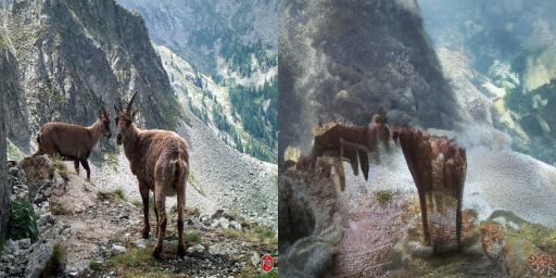
(a) alp $\rightarrow$ coral reef
on ImageNet with ResNet-50

(b) no-smile $\rightarrow$ smile
on CelebA HQ with DenseNet-121

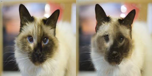
(c) birman $\rightarrow$ American pit bull
on Oxford Pets with OpenCLIP

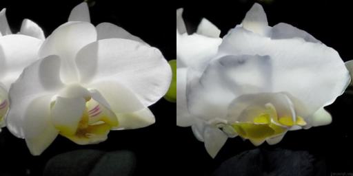
(d) moon orchid $\rightarrow$ rose
on Oxford Flowers with DINO+linear

Figure 1: LDCE(-txt) can be applied to any classifier, is dataset-agnostic, and works across various learning paradigms. We show counterfactual explanations (right) for the original image (left) for various dataset and classifier combinations.

2 Background

2.1 Diffusion models

Recent work showed that diffusion models can generate high-quality images (Sohl-Dickstein et al., 2015; Song & Ermon, 2019; Ho et al., 2020; Song et al., 2021; Rombach et al., 2022). The main idea is to gradually add small amounts of Gaussian noise to the data in the forward diffusion process and gradually undoing it in the learned reverse diffusion process. Specifically, given scalar noise scales $\{\alpha_{t}\}_{t=1}^{T}$ and an initial, clean image $x_{0}$, the forward diffusion process generates intermediate noisy representations $\{x_{t}\}_{t=1}^{T}$, with $T$ denoting the number of time steps. We can compute $x_{t}$ by

$$x_{t}=\sqrt{\alpha_{t}}x_{0}+\sqrt{1-\alpha_{t}}\epsilon_{t},\quad\textrm{where}\quad\epsilon_{t}\sim\mathcal{N}(\mathbf{0},\mathbf{I})\qquad.$$ (2)

The score estimator (i.e., parameterized denoising network) $\epsilon_{\theta}(x_{t},\;t)$–typically a modified U-Net (Ronneberger et al., 2015)–learns to undo the forward diffusion process for a pair $(x_{t},\;t)$:

$$\epsilon_{\theta}(x_{t},\;t)\approx\hat{\epsilon}_{t}=\frac{x_{t}-\sqrt{\alpha_{t}}x_{0}}{\sqrt{1-\alpha_{t}}}\quad.$$ (3)

Note that by rewriting Equation 3 (or 2), we can approximately predict the clean data point

$$\hat{x}_{0}\approx\frac{x_{t}-\sqrt{1-\alpha_{t}}\epsilon_{\theta}(x_{t},\;t)}{\sqrt{\alpha_{t}}}\quad.$$ (4)

To gradually denoise, we can sample the next less noisy representation $x_{t-1}$ with a sampling method $S(x_{t},\;\hat{\epsilon}_{t},\;t)\rightarrow x_{t-1}$, such as the DDIM sampler (Song et al., 2021):

$$x_{t-1}=\sqrt{\alpha_{t-1}}\frac{x_{t}-\sqrt{1-\alpha_{t}}\hat{\epsilon}_{t}}{\sqrt{\alpha_{t}}}+\sqrt{1-\alpha_{t-1}-\sigma^{2}_{t}}\hat{\epsilon}_{t}+\sigma_{t}\epsilon_{t}\quad.$$ (5)

Latent diffusion models

In contrast to GANs (Goodfellow et al., 2020), VAEs (Kingma & Welling, 2014; Rezende et al., 2014), or normalizing flows (Rezende & Mohamed, 2015), (pixel-space) diffusion models’ intermediate representations are high-dimensional, rendering the generative process computationally very intensive. To mitigate this, Rombach et al. (2022) proposed to operate diffusion models in a perceptually equivalent, lower-dimensional latent space $\mathcal{Z}$ of a regularized autoencoder $\mathcal{A}(x)=\mathcal{D}(\mathcal{E}(x))\approx x$ with encoder $\mathcal{E}$ and decoder $\mathcal{D}$ (Esser et al., 2021). Note that this also decouples semantic from perceptual compression s.t. the “focus [of the diffusion model is] on the important, semantic bits of the data” (Rombach et al. (2022), p. 4).

Controlled image generation

To condition the generation by some condition $c$, a class label or text, we need to learn a score function $\nabla_{x}\log p(x|c)$. Through, Bayes’ rule we can decompose the score function into an unconditional and conditional component:

$$\nabla_{x}\log p_{\eta}(x|c)=\nabla_{x}\log p(x)+\eta\nabla_{x}\log p(c|x)\quad,$$ (6)

where the guidance scale $\eta$ governs the influence of the conditioning signal. Note that $\nabla_{x}\log p(x)$ is just the unconditional score function and $\nabla_{x}\log p(c|x)$ can be a standard classifier. However, intermediate representations of the diffusion process have high noise levels and directly using a classifier’s gradient may result in mere adversarial perturbations (Augustin et al., 2022). To overcome this, previous work used noise-aware classifiers (Dhariwal & Nichol, 2021), optimized intermediate representation of the diffusion process (Jeanneret et al., 2023; Wallace et al., 2023), or used one-step approximations (Avrahami et al., 2022; Augustin et al., 2022; Bansal et al., 2023). In contrast to these works, Ho & Salimans (2022) trained a conditional diffusion model $\nabla_{x}\log p(x|c)$ with conditioning dropout and leveraged Bayes’ rule, i.e.,

$$\nabla_{x}\log p(c|x)=\nabla_{x}\log p(x|c)-\nabla_{x}\log p(x)\quad,$$ (7)

to substitute the conditioning component $\nabla_{x}\log p(c|x)$ from Equation 6:

$$\nabla_{x}\log p_{\eta}(x|c)=\nabla_{x}\log p(x)+\eta(\nabla_{x}\log p(x|c)-\nabla_{x}\log p(x))\quad.$$ (8)

2.2 Counterfactual explanations

A counterfactual explanation $x^{\textrm{CF}}$ is a sample with the smallest and semantically meaningful change to an original factual input $x^{\textrm{F}}$ in order to achieve a desired output. In contrast to adversarial attacks, counterfactual explanations focus on semantic (i.e., human comprehensible) changes. Initial works on visual counterfactual explanations used gradient-based approaches (Wachter et al., 2017; Santurkar et al., 2019; Boreiko et al., 2022) or restricted the set of image manipulations (Goyal et al., 2019; Akula et al., 2020; Wang et al., 2021; Van Looveren & Klaise, 2021; Vandenhende et al., 2022). Other works leveraged invertible networks (Hvilshøj et al., 2021), deep image priors (Thiagarajan et al., 2021), or used generative models to regularize towards the image manifold to generate high-quality visual counterfactual explanations (Samangouei et al., 2018; Lang et al., 2021; Sauer & Geiger, 2021; Rodriguez et al., 2021; Khorram & Fuxin, 2022; Jacob et al., 2022). Recent works also adopted (pixel-space) diffusion models due to their remarkable generative capabilities (Sanchez & Tsaftaris, 2022; Jeanneret et al., 2022; 2023; Augustin et al., 2022).

3 Latent diffusion counterfactual explanations (LDCE)

  Input: (f)actual image $x^{\textrm{F}}$, condition $c$, target model $f$, encoder $\mathcal{E}$, decoder $\mathcal{D}$, sampler $S$, distance function $d$, “where” function $\phi$, consensus threshold $\gamma$, time steps $T$, weighing factors $\eta,\;\lambda_{c},~{}\lambda_{d}$

  Output: counterfactual image $x^{\textrm{CF}}$

  $z_{T}\leftarrow\sqrt{\alpha_{t}}\mathcal{E}(x^{F})+\sqrt{1-\alpha_{t}}\epsilon_{t},\quad\textrm{where}\quad\epsilon_{t}\sim\mathcal{N}(\mathbf{0},\mathbf{I})\quad\textrm{// c.f.\hbox{}, Equation~{}\ref{eq:forward_diffusion}}$

  for $t=T,\;\dots,\;0$ do

     $\epsilon_{uc},\;\epsilon_{c}\leftarrow\epsilon_{\theta}(z_{t},\;t,\;\varnothing),\epsilon_{\theta}(z_{t},\;t,\;c)\;$

     $\hat{x}_{0}\leftarrow\mathcal{D}(\frac{z_{t}-\sqrt{1-\alpha_{t}}\epsilon_{uc}}{\sqrt{\alpha_{t}}})\quad\textrm{// c.f.\hbox{}, Equation~{}\ref{eq:DDIM_x0}}$

     $\texttt{cls\_score},\;\texttt{dist\_score}\leftarrow\sqrt{1-\alpha_{t}}\nabla_{z_{t}}\mathcal{L}(f(\hat{x}_{0}),\;c),\;\sqrt{1-\alpha_{t}}\nabla_{z_{t}}d(\hat{x}_{0},x^{\textrm{F}})$

     $\alpha_{i}\leftarrow\angle(\texttt{cls\_score}_{i},(\epsilon_{c}-\epsilon_{uc})_{i})$

     $\texttt{consensus}\leftarrow\phi(\alpha_{i},\;\gamma,\;\texttt{cls\_score}_{i},\;\mathbf{0})$

     $\hat{\epsilon}_{t}\leftarrow\epsilon_{uc}+\eta\cdot(\lambda_{c}\frac{\texttt{consensus}}{||\texttt{consensus}||_{2}}+\lambda_{d}\frac{\texttt{dist\_score}}{||\texttt{dist\_score}||_{2}})\cdot||\epsilon_{c}||_{2}$

     $z_{t-1}\leftarrow S(z_{t},\;\hat{\epsilon}_{t},\;t)\quad\textrm{// e.g.\hbox{}, Equation~{}\ref{eq:ddim_sampler}}$

  end for

  $x^{\textrm{CF}}\leftarrow\mathcal{D}(z_{0})$

Algorithm 1 Latent diffusion counterfactual explanations (LDCE).

Since generating (visual) counterfactual explanations $x^{\textrm{CF}}$ is inherently challenging due to high chance of adversarial perturbation by solely relying on the target model’s gradient, recent work resorted to (pixel-space) diffusion models to regularize counterfactual generation towards the data manifold by employing the following two-step procedure:

1. Abduction: add noise to the (f)actual image $x^{\textrm{F}}$ through the forward diffusion process, and

2. Interventional generation: guide the noisy intermediate representations by the gradients, or a projection thereof, from the target model $f$ s.t. the counterfactual $x^{\textrm{CF}}$ elicits a desired output $y^{\mathrm{CF}}$ from $f$.

Since intermediate representations of the diffusion model have high-noise levels and may result in mere adversarial perturbations, previous work proposed several schemes to combat these. This included sharing the encoder between target model and denoising network (Diff-SCM, Sanchez & Tsaftaris (2022)), albeit at the cost of model-specificity. Other work (DiME, Jeanneret et al. (2022) & ACE, Jeanneret et al. (2023)) proposed a computationally intensive iterative approach, where at each diffusion time step, they generated an unconditional, clean image to compute gradients on these unnoisy images, but necessitating backpropagation through the entire diffusion process up to the current time step. This results in computational costs of $\mathcal{O}(T^{2})$ or $\mathcal{O}(T\cdot I)$ for DiME or ACE, respectively, where $T$ is the number of diffusion steps and $I$ is the number of adversarial attack update steps in ACE. Lastly, Augustin et al. (2022) (DVCE) introduced a guidance scheme involving a projection between the target model and an auxiliary adversarially robust model. However, this requires the auxiliary model to be trained on a very similar data distribution (and task), which may limit its applicability in settings with restricted data access. Further, we found that counterfactuals generated by DVCE are confounded by the auxiliary model; see Appendix A for an extended discussion or Figure 3 of Augustin et al. (2022).

3.1 Overview

We propose Latent Diffusion Counterfactual Explanations (LDCE) that addresses above limitations: LDCE is model-agnostic, computationally efficient, and alleviates the need for an auxiliary classifier requiring (data-specific, adversarial) training. LDCE harnesses the capabilities of recent class- or text-conditional foundation (latent) diffusion models, augmented with a novel consensus guidance mechanism (Section 3.2). The foundational nature of the text-conditional (latent) diffusion model grants LDCE the versatility to be applied across diverse models, datasets (within reasonable bounds), and learning paradigms, as illustrated in Figure 1. Further, we expedite counterfactual generation by operating diffusion models within a perceptually equivalent, semantic latent space, as proposed by Rombach et al. (2022). This also allows LDCE to “focus on the important, semantic [instead of unimportant, high-frequency details] of the data” (Rombach et al. (2022), p. 4). Moreover, our novel consensus guidance mechanism ensures semantically meaningful changes during the reverse diffusion process by leveraging the implicit classifier (Ho & Salimans, 2022) of class- or text-conditional foundation diffusion models as a filter. Lastly, note that LDCE is compatible to and will benefit from future advancements of diffusion models. Algorithm 1 provides the implementation outline, which will be described in detail below.

Counterfactual generation in latent space

We propose generating counterfactual explanations within a perceptually equivalent, lower-dimensional latent space of an autoencoder (Esser et al., 2021) and rewrite Equation 1 as follows:

$$x^{\textrm{CF}}=\mathcal{D}(z^{\prime})\in\operatorname*{arg\,min}\limits_{z^{\prime}\in\mathcal{Z}=\{\mathcal{E}(x)|x\in\mathcal{X}\}}\lambda_{c}\mathcal{L}(f(\mathcal{D}(z^{\prime})),\;y^{\textrm{CF}})+\lambda_{d}d(\mathcal{D}(z^{\prime}),\;x^{\textrm{F}})\quad.$$ (9)

Yet, we found that generating counterfactual explanations directly in the autoencoder’s latent space (Esser et al., 2021) using a gradient-based approach only results in imperceptible, adversarial changes. Conversely, employing a diffusion model on the latent space produced semantically more meaningful changes. Further, it allows the diffusion model to “focus on the important, semantic bits of the data” (Rombach et al. (2022), p. 4) and the autoencoder’s decoder $\mathcal{D}$ fills in the unimportant, high-frequency image details. This contrasts prior works that used pixel-space diffusion models for counterfactual generation. We refer to this approach as LDCE-no consensus.

3.2 Consensus guidance mechanism

Figure 2: Our proposed consensus guidance mechanism employs a filtering approach of gradients leveraging the implicit classifier of diffusion models as reference for semantic meaningfulness.

To further mitigate the presence of semantically non-meaningful changes, we introduce a novel consensus guidance mechanism (see Figure 2). During the reverse diffusion process, our guidance mechanism exclusively allows for gradients from the target model that align with the freely available implicit classifier of a class- or text-conditional diffusion model (c.f., Equation 7). Consequently, we can use target models out-of-the-box and eliminate the need for auxiliary models that need to be (adversarially) trained on a similar data distribution (and task). We denote these variants as LDCE-cls for class-conditional or LDCE-txt for text-conditional diffusion models, respectively.

Our consensus guidance mechanism is inspired by the observation that both the gradient of the target model, and the unconditional and conditional score functions of the class- or text-conditional foundation diffusion model (c.f., Equation 7) estimate $\nabla_{x}\log p(c|x)$. The main idea of our consensus guidance mechanism is to leverage the latter as a reference for semantic meaningfulness to filter out misaligned gradients of the target model that are likely to result in non-meaningful, adversarial modifications. More specifically, we compute the angles $\alpha_{i}$ between the target model’s gradients $\nabla_{z_{t}}\mathcal{L}(f(\hat{x}_{0}),\;c)$ and the difference of the conditional and unconditional scores $\epsilon_{c}-\epsilon_{uc}$ (c.f., Equation 7) for each non-overlapping patch, indexed by $i$:

$$\alpha_{i}=\angle[(\sqrt{1-\alpha_{t}}\nabla_{z_{t}}\mathcal{L}(f(\hat{x}_{0}),\;c))_{i},\;(\epsilon_{c}-\epsilon_{uc})_{i}]\quad.$$ (10)

To selectively en- or disable gradients for individual patches, we introduce an angular threshold $\gamma$:

$$\phi_{i}(\alpha_{i},\;\gamma,\;\sqrt{1-\alpha_{t}}\nabla_{z_{t}}\mathcal{L}(f(\hat{x}_{0}),\;c))_{i},\;\mathbf{o})=\left\{\begin{array}[]{ll}\sqrt{1-\alpha_{t}}\nabla_{z_{t}}\mathcal{L}(f(\hat{x}_{0}),\;c))_{i},&\alpha_{i}\leq\gamma\\ \mathbf{o},&\alpha_{i}>\gamma\end{array}\right.,$$ (11)

where $\mathbf{o}$ is the overwrite value (in our case zeros $\mathbf{0}$). Note that by setting the overwrite value $\mathbf{o}$ to zeros, only the target model and the unconditional score estimator–which is needed for regularization towards the data manifold–directly influence counterfactual generation.

4 Experiments

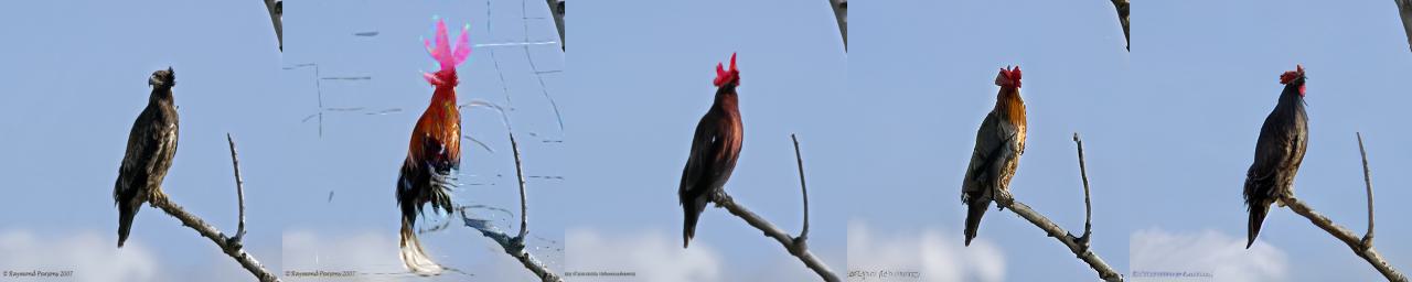
(a) bald eagle $\rightarrow$ rooster

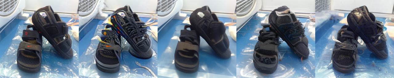
(b) sandal $\rightarrow$ running shoe

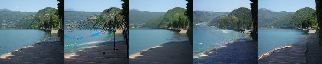
(c) lakeside $\rightarrow$ seashore

(d) barn $\rightarrow$ planetarium

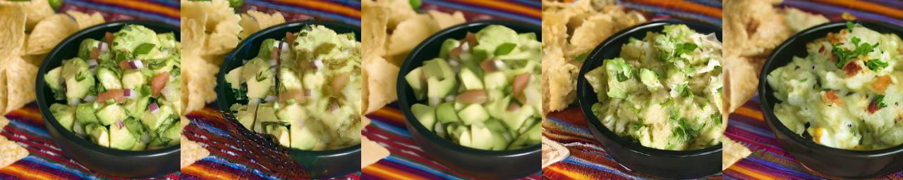
(e) guacamole $\rightarrow$ mashed potato

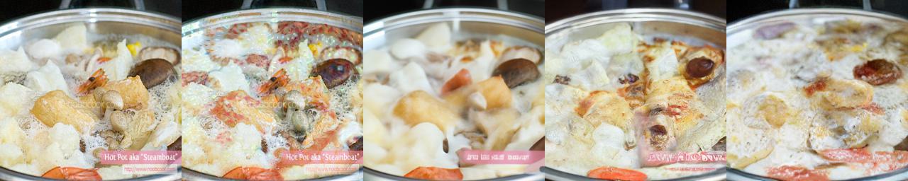
(f) hot pot $\rightarrow$ pizza

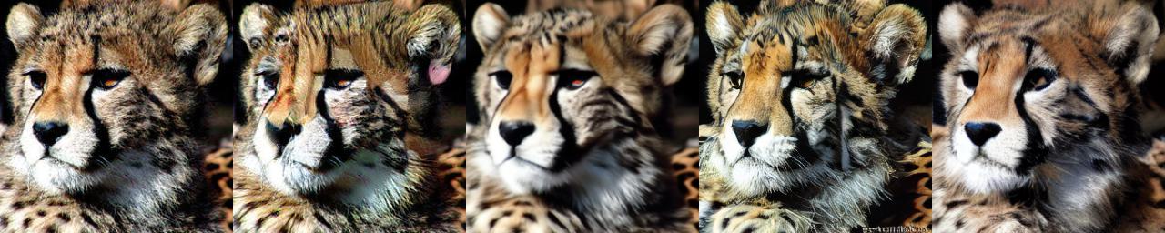
(g) cheetah $\rightarrow$ tiger

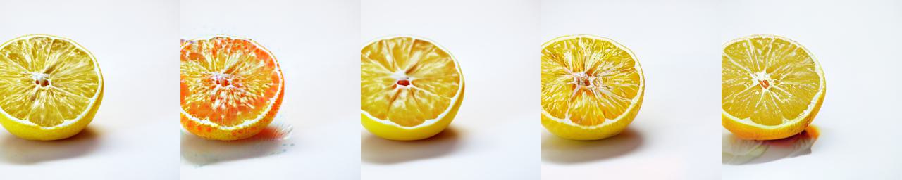
(h) lemon $\rightarrow$ orange

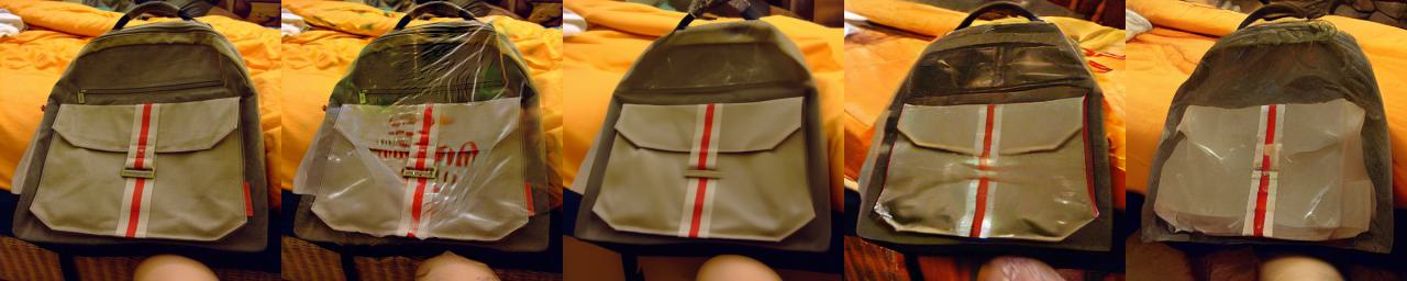
(i) backpack $\rightarrow$ plastic bag

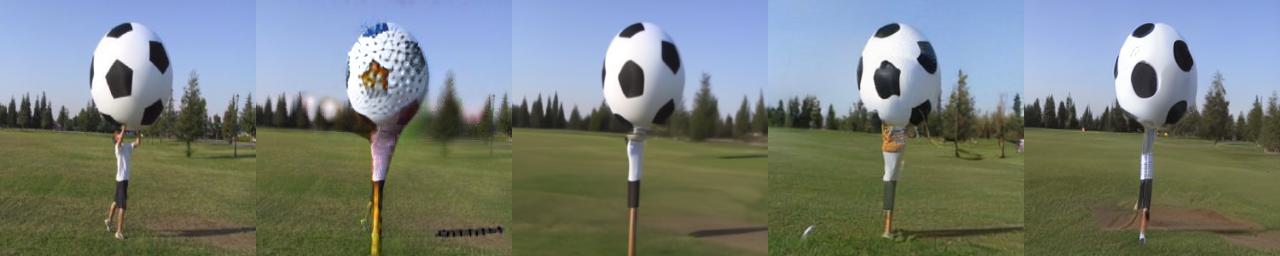
(j) soccer ball $\rightarrow$ golf ball

Figure 3: Qualitative comparison on ImageNet with ResNet-50. Left to right: original image, counterfactual images for SVCE, DVCE, LDCE-cls, and LDCE-txt. Appendix I provides more examples.

Datasets & models

We evaluated (and compared) LDCE on ImageNet (Deng et al., 2009) (on a subset of 10k images), CelebA HQ (Lee et al., 2020), Oxford Flowers 102 (Nilsback & Zisserman, 2008), and Oxford Pets (Parkhi et al., 2012). All datasets have image resolutions of 256x256. We used ResNet-50 (He et al., 2016), DenseNet-121 (Huang et al., 2017), OpenCLIP-VIT-B/32 (Cherti et al., 2022), and (frozen) DINO-VIT-S/8 with linear classifier (Caron et al., 2021) for ImageNet, CelebA HQ, Oxford Pets or Flowers 102, respectively, as target models. We provide dataset and model licenses in Appendix B and further model details in Appendix C.

Evaluation protocol

We use two protocols for counterfactual target class selection: (a) Semantic Hierarchy: we randomly sample one of the top-4 closest classes based on the shortest path based on WordNet (Miller, 1995). (b) Representational Similarity: we compute the instance-wise cosine similarity with SimSiam (Chen & He, 2021) features of the (f)actual images $x^{\mathrm{F}}$ and randomly sample one of the top-5 classes. Note that the latter procedure does not require any domain expertise compared to the former. We adopted the former for ImageNet and the latter for Oxford Pets and Flowers 102. For CelebA HQ, we selected the opposite binary target class.

The evaluation of (visual) counterfactual explanations is inherently challenging: what makes a good counterfactual is arguably very subjective. Despite this, we used various quantitative evaluation criteria covering commonly acknowledged desiderata. (a) Validity: We used Flip Ratio (FR), i.e., does the generated counterfactual $x^{\mathrm{CF}}$ yield the desired output $y^{\mathrm{CF}}$, and COUT (Khorram & Fuxin, 2022) that additionally takes the sparsity of the changes into account. Further, we used the $S^{3}$ criterion (Jeanneret et al., 2023) that computes cosine similarity between the (f)actual $x^{\textrm{F}}$ and counterfactual $x^{\textrm{CF}}$. While it has been originally introduced a closeness criterion, we found that $S^{3}$ correlates strongly with FR, i.e., we found a high Spearman rank correlation of $-0.83$ using the numbers from Table 2. (b) Closeness: We used L1 and L2 norms to assess closeness. However, note that L$p$ norms can be confounded by unimportant, high-level image details. (c) Realism: We used FID and sFID (Jeanneret et al., 2023) to assess realism. In contrast to FID, sFID removes the bias caused by the closeness desiderata. Appendix D provides more details.

Implementation details

We based LDCE-cls on a class-conditional latent diffusion model trained on ImageNet (Rombach et al., 2022) and LDCE-txt on a fine-tuned variant of Stable Diffusion v1.4 for 256x256 images (Pinkey, 2023). Model licenses and links to the weights are provided in Appendix B. For text conditioning, we mapped counterfactual target classes to CLIP-style text prompts (Radford et al., 2021). For our consensus guidance scheme, we used spatial regions of size 1x1 and chose zeros as overwrite values. We used L1 as a distance function $d$ to promote sparse changes. We used a diffusion respacing factor of 2 to expedite counterfactual generation at the cost of a reduction in image quality. We set the weighting factor $\eta$ to 2. We optimized other hyperparameters (diffusion steps $T$ and the other weighing factors $\lambda_{c},\;\gamma,\;\lambda_{d}$) on 10–20 examples. Note that these hyperparameters control the trade-off of the desiderata validity, closeness, and realism. Appendix E provides the selected hyperparameters.

4.1 Qualitative evaluation

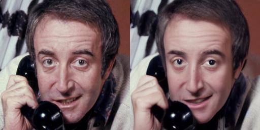
(a) young $\rightarrow$ old

(b) old $\rightarrow$ young

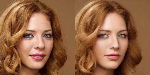
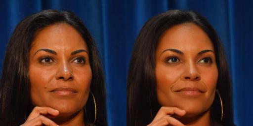
(c) smile $\rightarrow$ no smile

(d) no smile $\rightarrow$ smile

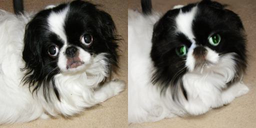
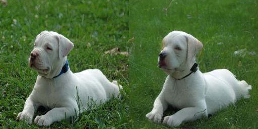
(e) jpn. chin $\rightarrow$ persian cat

(f) am. bulldog $\rightarrow$ beagle

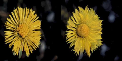
(g) coltsfoot $\rightarrow$ sunflower

(h) pink primrose $\rightarrow$ lotus

Figure 4: Qualitative results on CelebA HQ, Oxford Pets, and Flowers 102 using DenseNet-121, CLIP, and DINO with linear classifier, respectively. Left: original image. Right: counterfactual image generated by LDCE-txt. Additional examples are provided in Appendix I.

Figures 1, 3, and 4 show qualitative results for both LDCE-cls and LDCE-txt across a diverse range of models (from convolutional networks to transformers) trained on various real-world datasets (from ImageNet to CelebA-HQ, Oxford-Pets, or Flowers-102) with distinct learning paradigms (from supervision, to vision-only or vision-language self-supervision). We observe that LDCE-txt can introduce local changes, e.g., see Figure 1(b), as well as global modifications, e.g., see Figure 1(a). We observe similar local as well as global changes for LDCE-cls in Figure 3. Notably, LDCE-txt can also introduce intricate changes in the geometry of flower petals without being explicitly trained on such data, see Figure 1(d) or the rightmost column of Figure 4. Further, we found that counterfactual generation gradually evolves from coarse (low-frequency) features (e.g., blobs or shapes) at the earlier time steps towards more intricate (high-frequency) details (e.g., textures) at later time steps. We explores this further in Appendix F. Lastly, both LDCE variants can generate a diverse set of counterfactuals, instead of only single instances, by introducing stochasticity in the abduction step (see Appendix G for examples).

Figure 3 also compares LDCE with previous works: SVCE (Boreiko et al., 2022) and DVCE (Augustin et al., 2022). We found that SVCE often generates high-frequency (Figure 3(c)) or copy-paste-like artifacts (Figure 3(e)). Further, DVCE tends to generate blurry and lower-quality images. This is also reflected in its worse (s)FID scores in Table 1. Moreover, note that counterfactuals generated by DVCE are confounded by its auxiliary model; refer to Appendix A for an extended discussion. In contrast to SVCE and DVCE, both LDCE variants generate fewer artifacts, less blurry, and higher-quality counterfactual explanations. However, we also observed failure modes (e.g., distorted secondary objects) and provide examples in Appendix K. We suspect that some of these limitations are inherited from the underlying foundation diffusion model and, in part, to domain shift. We further discuss these challenges in Section 5.

4.2 Quantitative evaluation

Table 1: Comparison to SVCE and DVCE on ImageNet using ResNet-50.

Method	L1 ($\downarrow$)	L2 ($\downarrow$)	FID ($\downarrow$)	sFID ($\downarrow$)	FR ($\uparrow$)
$\ell_{1.5}$-SVCE† (Boreiko et al., 2022)	5038	25	22.44	28.44	83.82
DVCE (Augustin et al., 2022)	6453	24	23.94	28.99	84.0
LDCE-no consensus	12337	41	21.70	27.10	98.4
LDCE-cls	12375	42	14.03	19.25	83.1
LDCE-txt∗	11577	41	21.00	26.50	84.4
†: used an adversarially robust ResNet-50. ∗: diffusion model not trained on ImageNet.

We quantitatively compared LDCE to previous work ($\ell_{1.5}$-SVCE (Boreiko et al., 2022), DVCE (Augustin et al., 2022), and ACE (Jeanneret et al., 2023)) on ImageNet. Note that other previous work is hardly applicable to ImageNet or code is not provided, e.g., C3LT (Khorram & Fuxin, 2022). Note that we used a multiple-norm robust ResNet-50 (Croce & Hein, 2021) for $\ell_{1.5}$-SVCE since it is tailored for adversarially robust models. Further, we limited our comparison to ACE to their smaller evaluation protocol for ImageNet due to its computationally intensive nature.

Table 2: Comparison of LDCE-cls and LDCE-txt (^∗diffusion model not trained on ImageNet) to ACE on ImageNet with ResNet-50.

Method	FID	sFID	S3	COUT	FR
Zebra – Sorrel
ACE $\ell_{1}$	84.5	122.7	0.92	-0.45	47.0
ACE $\ell_{2}$	67.7	98.4	0.90	-0.25	81.0
LDCE-cls	84.2	107.2	0.78	-0.06	88.0
LDCE-txt∗	82.4	107.2	0.7113	-0.2097	81.0
Cheetah – Cougar
ACE $\ell_{1}$	70.2	100.5	0.91	0.02	77.0
ACE $\ell_{2}$	74.1	102.5	0.88	0.12	95.0
LDCE-cls	71.0	91.8	0.62	0.51	100.0
LDCE-txt∗	91.2	117.0	0.59	0.34	98.0
Egyptian Cat – Persian Cat
ACE $\ell_{1}$	93.6	156.7	0.85	0.25	85.0
ACE $\ell_{2}$	107.3	160.4	0.78	0.34	97.0
LDCE-cls	102.7	140.7	0.63	0.52	99.0
LDCE-txt∗	121.7	162.4	0.61	0.56	99.0

Table 1 shows that both LDCE variants achieve strong performance for the validity (high FR) and realism (low FID figures) desiderata. Unsurprisingly, we find that SVCE generates counterfactuals that are closer to the (f)actual image (lower L$p$ norms) since it specifically constraints optimization within a $\ell_{1.5}$-ball. We also note that unsurprisingly L$p$ norms are higher for both LDCE variants than for the other methods since L$p$ are confounded by unimportant, high-frequency image details that are not part of our counterfactual optimization, i.e., the decoder just fills in these details. This is corroborated by our qualitative inspection in Section 4.1. Furthermore, we found that both LDCE variants consistently outperform ACE across nearly all evaluation criteria; see Table 2. The only exception is FID, which is unsurprising given that ACE enforces sparse changes, resulting in counterfactuals that remain close to the (f)actual images. This is affirmed by ACE’s lower sFID scores, which accounts for this. We provide quantitative comparisons with other methods on CelebA HQ in Appendix H. Despite not being trained specifically for faces, LDCE-txt yielded competitive results to other methods.

Lastly, we evaluated the computational efficiency of diffusion-based counterfactual methods. Specifically, we compared throughput on a single NVIDIA RTX 3090 GPU with $24\text{\,}\mathrm{GB}$ memory for 20 batches with maximal batch size. We report that LDCE-txt only required $156\text{\,}\mathrm{s}$ for four counterfactuals, whereas DVCE needed $210\text{\,}\mathrm{s}$ for four counterfactuals, and ACE took $184\text{\,}\mathrm{s}$ for just a single counterfactual. Note that DiME, by design, is even slower than ACE. Above throughput differences translate to substantial speed-ups of $34\text{\,}\mathrm{\%}$ and $371\text{\,}\mathrm{\%}$ compared to DVCE or ACE, respectively.

Above results highlight LDCE as a strong counterfactual generation method. In particular, LDCE-txt achieves on par and often superior performance compared to previous approaches, despite being the only method not requiring any component to be trained on the same data as the target model–a property that, to the best of our knowledge, has not been available in any previous work and also enables applicability in real-world scenarios where data access may be restricted.

4.3 Identification and resolution of model errors

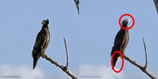
(a) kite $\rightarrow$ bald eagle

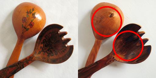
(b) maraca $\rightarrow$ wooden spoon

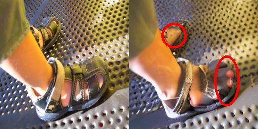
(c) running shoe $\rightarrow$ sandal

Figure 5: Examples of identified classification errors of ResNet-50. Left: original image that is misclassified. Right: counterfactual that is correctly classified. The red ellipses were added manually.

Counterfactual explanations should not solely generate high-quality images, like standard image generation, editing or prompt-to-prompt methods (Hertz et al., 2023), but should serve to better understand model behavior. More specifically, we showcase how LDCE-txt can effectively enhance our model understanding of ResNet-50 trained with supervision on ImageNet in the context of misclassifications. To this end, we generated counterfactual explanations of a ResNet-50’s misclassifications towards the true class. As illustrated in Figure 5, this elucidates missing or misleading features in the original image that lead to a misclassification. For instance, it reveals that ResNet-50 may misclassify young bald eagles primarily due to the absence of their distinctive white heads (and tails), which have yet to fully develop. Similarly, we found that painted wooden spoons may be misclassified as maraca, while closed-toe sandals may be confused with running shoes.

To confirm that these findings generalize beyond single instances, we first tried to synthesize images for each error type with InstructPix2Pix (Brooks et al., 2023), but found that it often could not follow the instructions; indicating that these model errors transcend ResNet-50 trained with supervision. Thus, we searched for 50 images on the internet, and report classification error rates of $88\text{\,}\mathrm{\%}$, $74\text{\,}\mathrm{\%}$, and $48\text{\,}\mathrm{\%}$ for the bald eagle, wooden spoon, or sandal model errors, respectively. Finally, we used these images to finetune the last linear layer of ResNet-50. To this end, we separated the 50 images into equally-sized train and test splits; finetuning details are provided in Appendix J. This effectively mitigated these model errors and reduced error rates on the test set by $40\text{\,}\mathrm{\%}$, $32\text{\,}\mathrm{\%}$, or $16\text{\,}\mathrm{\%}$, respectively.

5 Limitations

The main limitation of LDCE is its slow counterfactual generation, which hinders real-time, interactive applications. However, advancements in distilling diffusion models (Salimans & Ho, 2022; Song et al., 2023; Meng et al., 2023) or speed-up techniques (Dao et al., 2022; Bolya et al., 2023) offer promise in mitigating this limitation. Another limitation is the requirement for hyperparameter optimization. Although this is very swift, it still is necessary due to dataset differences and diverse needs in use cases. Lastly, while contemporary foundation diffusion models have expanded their data coverage (Schuhmann et al., 2021), they may not perform as effectively in specialized domains, e.g., for biomedical data, or may contain (social) biases (Bianchi et al., 2023; Luccioni et al., 2023).

6 Conclusion

We introduced LDCE to generate semantically meaningful counterfactual explanations using class- or text-conditional foundation (latent) diffusion models, combined with a novel consensus guidance mechanism. We show LDCE’s versatility across diverse models learned with diverse learning paradigms on diverse datasets, and demonstrate its applicability to better understand model errors and resolve them. Future work could employ our consensus guidance mechanism beyond counterfactual generation and incorporate spatial or textual priors.

Broader impact

Counterfactual explanations aid in understanding model behavior, can reveal model biases, etc. By incorporating latent diffusion models (Rombach et al., 2022), we make a step forward in reducing computational demands in the generation of counterfactual explanations. However, counterfactual explanations may be manipulated (Slack et al., 2021) or abused. Further, (social) biases in the foundation diffusion models (Bianchi et al., 2023; Luccioni et al., 2023) may also be reflected in counterfactual explanations, resulting in misleading explanations.

Author contributions

Project idea: S.S.; project lead: S.S. & K.F.; conceptualization of consensus guidance mechanism: K.F. with input from S.S.; method implementation: K.F. & S.S.; hyperparameter optimization: K.F.; implementation and execution of experiments: S.S. & K.F. with input from M.A. & T.B.; visualization: S.S. with input from K.F. (experimental results) & M.A. with input from S.S. & K.F. (Figure 2); interpretation of findings: K.F. & S.S. with input from M.A. & T.B.; guidance & feedback: M.A. & T.B.; funding acquisition: T.B.; paper writing: S.S. & K.F. crafted the first draft and all authors contributed to the final version.

Acknowledgments

This work was funded by the Bundesministerium für Umwelt, Naturschutz, nukleare Sicherheit und Verbraucherschutz (BMUV, German Federal Ministry for the Environment, Nature Conservation, Nuclear Safety and Consumer Protection) based on a resolution of the German Bundestag (67KI2029A) and the Deutsche Forschungsgemeinschaft (DFG, German Research Foundation) under grant number 417962828. K.F. acknowledges supported by the Deutscher Akademischer Austauschdienst (DAAD, German Academic Exchange Service) as part of the ELIZA program.

Appendix A Influence of the adversarial robust model in DVCE

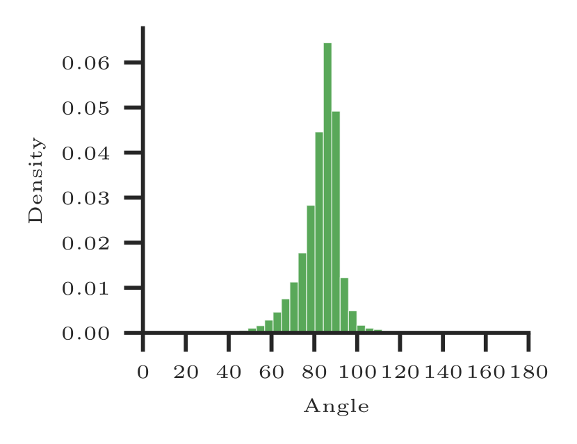
Figure 6: Distribution of angles between the gradient of the target and the robust classifier over 100 images over 100 timesteps.

DVCE (Augustin et al., 2022) uses a projection technique to promote semantically meaningful changes, i.e., they project the unit gradient of an adversarially robust model onto a cone around the unit gradient of the target model, when the gradient directions disagree, i.e., the angle between them exceeds an angular threshold $\alpha$. More specifically, Augustin et al. (2022) defined their cone projection as follows:

$$P_{\textrm{cone}(\alpha,v)}[w]:=\left\{\begin{array}[]{ll}\langle u,w\rangle u,&\angle(w,v)>\alpha\\ v,&\textrm{else}\end{array}\right.,$$ (12)

where $v,w$ are the unit gradients of the target classifier and adversarially robust classifier, respectively, $\textrm{cone}(\alpha,v):=\{w\in\mathbb{R}^{d}:\angle(v,w)\leq\alpha\}$, and

$$u=\sin{\alpha}\frac{P_{v^{\perp}}(w)}{||P_{v^{\perp}}(w)||_{2}}+\cos{\alpha}\frac{v}{||v||_{2}}\qquad,$$ (13)

where $P_{v^{\perp}(w)}:=w-\frac{\langle w,v\rangle}{\langle v,v\rangle}v$. However, due to the high dimensionality of the unit gradients ($\mathbb{R}^{256\cdot 256\cdot 3}$), they are nearly orthogonal with high probability. In fact, we empirically observed that ca. $97.73\text{\,}\mathrm{\%}$ of the gradients pairs have angles larger than 60^∘ during the counterfactual generation of 100 images from various classes; see Figure 6. As a result, we almost always use the cone projection and found that the counterfactuals are substantially influenced by the adversarially robust model: Figure 3 of Augustin et al. (2022) and Figure 7 highlight that the target model has a limited effect in shaping the counterfactuals. Consequently, we cannot attribute the changes of counterfactual explanations solely to the target model since they are confounded by the auxiliary adversarially robust model.

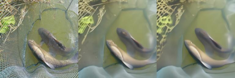
(a) tench $\rightarrow$ eel

(b) tiger shark $\rightarrow$ great white shark

(c) electric ray $\rightarrow$ great white shark

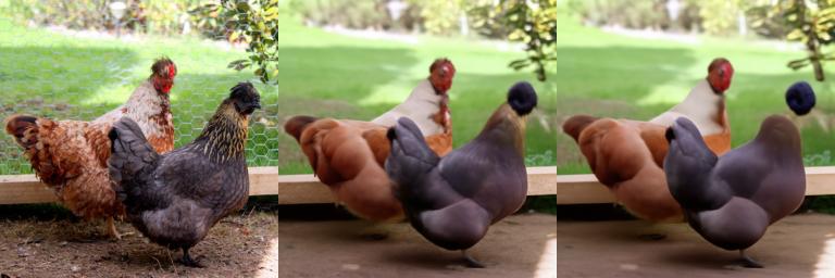
(d) hen $\rightarrow$ rooster

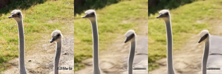
(e) ostrich $\rightarrow$ african grey

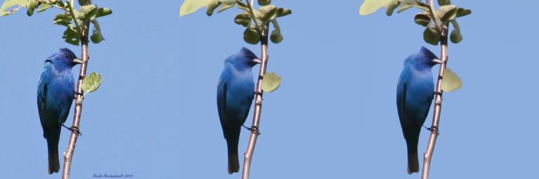
(f) indigo bunting $\rightarrow$ goldfinch

Figure 7: Qualitative examples illustrating the marginal influence of the target model in DVCE. From left to right: original image, counterfactual images generated using DVCE with cone projection using an angular threshold of $30^{\circ}$ and the robust classifier, and DVCE using the robust classifier only, i.e., without the target model.

Appendix B Dataset and model licenses

Table 3 and 4 provide licenses and URLs of the datasets or models, respectively, used in our work. Our implementation is built upon Rombach et al. (2022) (License: Open RAIL-M, URL: https://github.com/CompVis/stable-diffusion) and provided at https://github.com/lmb-freiburg/ldce (License: MIT).

Table 3: Licenses and URLs for the datasets used in our experiments.

Dataset	License	URL
CelebAMask-HQ (Lee et al., 2020)	CC BY 4.0	https://github.com/switchablenorms/CelebAMask-HQ
Oxford Flowers 102 (Nilsback & Zisserman, 2008)	GNU	https://www.robots.ox.ac.uk/~vgg/data/flowers/102/
ImageNet (Deng et al., 2009)	Custom	https://www.image-net.org/index.php
Oxford Pet (Parkhi et al., 2012)	CC BY-SA 4.0	https://www.robots.ox.ac.uk/~vgg/data/pets/

Table 4: Licenses and URLs for the target and diffusion models used in our experiments.

Models	License	URL
ImageNet class- conditional LDM (Rombach et al., 2022)	MIT	https://github.com/CompVis/latent-diffusion
Mini Stable diffusion 1.4 (Pinkey, 2023)	CreativeML Open RAIL-M (Rombach et al., 2022)	https://huggingface.co/justinpinkney/miniSD
ResNet-50 for ImageNet (He et al., 2016; TorchVision maintainers and contributors, 2016)	BSD 3	https://github.com/pytorch/vision
Adv. robust ResNet-50 for ImageNet (Boreiko et al., 2022)	MIT	https://github.com/valentyn1boreiko/SVCEs_code
DenseNet-121 (Huang et al., 2017) for CelebA HQ (Jacob et al., 2022)	Apache 2	https://github.com/valeoai/STEEX
DINO for Oxford Flowers 102 (Caron et al., 2021)	Apache 2	https://github.com/facebookresearch/dino
OpenCLIP for Oxford Pets (Cherti et al., 2022)	Custom	https://github.com/mlfoundations/open_clip
SimSiam (Chen & He, 2021)	CC BY-NC 4.0	https://github.com/facebookresearch/simsiam
CelebA HQ Oracle (Jacob et al., 2022)	Apache 2	https://github.com/valeoai/STEEX
Ported VGGFace2 model from (Cao et al., 2018)	MIT	https://github.com/cydonia999/VGGFace2-pytorch

Appendix C Model details

Below, we provide model details:

• ResNet50 (He et al., 2016) on ImageNet (Deng et al., 2009): We used the pretrained ResNet-50 model provided by torchvision (TorchVision maintainers and contributors, 2016).

• DenseNet-121 (Huang et al., 2017) on CelebA HQ (Lee et al., 2020): We used the pretrained DenseNet-121 model provided by Jacob et al. (2022).

• OpenCLIP (Radford et al., 2021; Cherti et al., 2022) on Oxford Pets (Parkhi et al., 2012): We used the provided weights of OpenCLIP ViT-B/32 (Dosovitskiy et al., 2021), and achieved a top-1 zero-shot classification accuracy of $90.5\text{\,}\mathrm{\%}$ using CLIP-style prompts (Radford et al., 2021).

• DINO+linear (Caron et al., 2021) on Oxford Flowers 102 (Nilsback & Zisserman, 2008): We used the pretrained DINO ViT-S/8 model, added a trainable linear classifier, and trained it on Oxford Flowers 102 for 30 epochs. We used SGD with a learning rate of 0.001 and momentum of 0.9, and cosine annealing (Loshchilov & Hutter, 2019). The model achieved a top-1 classification accuracy of $92.82\text{\,}\mathrm{\%}$.

Appendix D Evaluation criteria for counterfactual explanations

In this section, we discuss the evaluation criteria used to quantitatively assess the quality of counterfactual explanations. Even though quantitative assessment of counterfactual explanations is arguably very subjective, these evaluation criteria build a basis of quantitative evaluation based on the commonly recognized desiderata validity, closeness, and realism.

Flip Ratio (FR)

This criterion focuses on assessing the validity of $N$ counterfactual explanations by quantifying the degree to which the original class label $y_{i}^{\textrm{F}}$ of the original image $x_{i}^{\textrm{F}}$ flips the target classifier’s prediction $f$ to the counterfactual target class $y_{i}^{\textrm{CF}}$ for the counterfactual image $x_{i}^{\textrm{CF}}$:

$$\text{FR}=\frac{{\sum\limits_{i=1}^{N}\mathbb{I}(f(x^{\textrm{CF}}_{i})=y_{i}^{\textrm{CF}})}}{{N}}\qquad,$$ (14)

where $\mathbb{I}$ is the indicator function.

Counterfactual Transition (COUT)

Counterfactual Transition (COUT) (Khorram & Fuxin, 2022) measures the sparsity of changes in counterfactual explanations, incorporating validity and sparsity aspects. It quantifies the impact of perturbations introduced to the (f)actual image $x^{\textrm{F}}$ using a normalized mask $m$ that represents relative changes compared to the counterfactual image $x^{\textrm{CF}}$, i.e., $m=\delta(||x^{\textrm{F}}-x^{\textrm{CF}}||_{1})$, where $\delta$ normalizes the absolute difference to $[0,1]$. We progressively perturb $x^{\textrm{F}}$ by inserting top-ranked pixel batches from $x^{\textrm{CF}}$ based on these sorted mask values.

For each perturbation step $t\in\{0,\ldots,T\}$, we record the output scores of the classifier $f$ for the (f)actual class $y^{\textrm{F}}$ and the counterfactual class $y^{\textrm{CF}}$ throughout the transition from $x^{0}=x^{\textrm{F}}$ to $x^{T}=x^{\textrm{CF}}$. From this, we can compute the COUT score:

$$\textrm{COUT}=\textrm{AUPC}(y^{\textrm{CF}})-\textrm{AUPC}(y^{\textrm{F}})\in[-1,1]\qquad,$$ (15)

where the area under the Perturbation Curve (AUPC) for each class $y\in\{y^{\textrm{F}},y^{\textrm{CF}}\}$ is defined as follows:

$$\textrm{AUPC}(y)=\frac{1}{T}\sum_{t=0}^{T-1}\frac{1}{2}\left(f_{y}\left(x^{(t)}\right)+f_{y}\left(x^{(t+1)}\right)\right)\in[0,1]\qquad.$$ (16)

A high COUT score indicates that a counterfactual generation approach finds sparse changes that flip classifiers’ output to the counterfactual class.

SimSiam Similarity (S3)

This criterion measures the cosine similarity between a counterfactual image $x^{\textrm{CF}}$ and its corresponding (f)actual image $x^{\textrm{F}}$ in the feature space of a self-supervised SimSiam model $S$ (Chen & He, 2021):

$${S^{3}(x^{\textrm{CF}},x^{\textrm{F}})=\frac{{\mathcal{S}(x^{\textrm{CF}})\cdot\mathcal{S}(x^{\textrm{F}})}}{{\lVert\mathcal{S}(x^{\textrm{CF}})\rVert\lVert\mathcal{S}(x^{\textrm{F}})\rVert}}}\quad.$$ (17)

Lp norms

$Lp$ norms serve as closeness criteria by quantifying the magnitude of the changes between the counterfactual image $x_{i}^{\textrm{CF}}$ and original image $x_{i}^{\textrm{F}}$:

$$L_{p}=\frac{1}{N}\sum_{i=1}^{N}\|d_{i}\|_{p}\qquad,$$ (18)

where $0<p\leq\infty$ and $C,H,W$ are the number of channels, image height, and image width, respectively, and

$$\|d_{i}\|_{p}=\left(\sum_{c=1}^{C}\sum_{h=1}^{H}\sum_{w=1}^{W}|x_{i,c,h,w}^{\textrm{F}}-x_{i,c,h,w}^{\textrm{CF}}|^{p}\right)^{\frac{1}{p}}\qquad.$$ (19)

Note that $Lp$ norms can be confounded by unimportant, high-frequency image details.

Mean Number of Attribute Changes (MNAC)

Mean Number of Attribute Changes (MNAC) quantifies the average number of attributes modified in the generated counterfactual explanations. It uses an oracle model $O_{a}$ (i.e., VGGFace2 model (Cao et al., 2018)) which predicts the probability of each attribute $a\in\mathcal{A}$, where $\mathcal{A}$ is the entire attributes space. MNAC is defined as follows:

$$\text{MNAC}=\frac{1}{N}\sum_{i=1}^{N}\sum_{a\in\mathcal{A}}\left[\mathbb{I}\left(\mathbb{I}\left(O_{a}(x^{\textrm{CF}}_{i})>\beta\right)\neq\mathbb{I}\left(O_{a}(x^{\textrm{F}}_{i})>\beta\right)\right)\right]\qquad,$$ (20)

where ${\beta}$ is a threshold (typically set to 0.5) that determines the presence of attributes. MNAC quantifies the counterfactual method’s changes to the query attribute $q$, while remaining independent of other attributes. However, a higher MNAC value can wrongly assign accountability for spurious correlations to the counterfactual approach, when in fact they may be artifacts of the classifier.

Correlation Difference (CD)

Correlation Difference (CD) (Jeanneret et al., 2022) evaluates the ability of counterfactual methods to identify spurious correlations by comparing the Pearson correlation coefficient $c^{q,a}(x)$, of the relative attribute changes $\delta^{q}$ and $\delta^{a}$, before and after applying the counterfactual method. For each attribute $a$, the attribute change $\delta^{a}$ is computed between pairs of samples $i$ and $j$, as $\delta^{a}_{i,j}=\hat{y}^{a}_{i}-\hat{y}^{a}_{j}$, using the predicted probabilities $\hat{y}^{a}_{i}$ and $\hat{y}^{a}_{j}$ from the oracle model $O$ (i.e., VGGFace2 model (Cao et al., 2018)). The CD for a query attribute $q$ is then computed as:

$$\textrm{CD}_{q}=\frac{1}{N}\sum_{i=1}^{N}\sum_{a\in\mathcal{A}}|c^{q,a}(x^{\textrm{CF}})-c^{q,a}(x^{\textrm{F}})|\qquad.$$ (21)

Face Verification Accuracy (FVA) & Face Similarity (FS)

Face Verification Accuracy (FVA) quantifies whether counterfactual explanations for face attributes maintain identity while modifying the target attribute using the VGGFace2 model (Cao et al., 2018), or not. Alternatively, Jeanneret et al. (2023) proposed Face Similarity (FS) that addresses thresholding issues and the abrupt transitions in classifier decisions in FVA when comparing the (f)actual image $x^{\textrm{F}}$ and its corresponding counterfactual $x^{\textrm{CF}}$. FS directly measures the cosine similarity between the feature encodings, providing a more continuous assessment (similar to S³).

Fréchet Inception Distances (FID & sFID)

Fréchet Inception Distance (FID) (Heusel et al., 2017) and split FID (sFID) (Jeanneret et al., 2023) evaluate the realism of generated counterfactual images by measuring the distance on the dataset level between the InceptionV3 (Szegedy et al., 2016) feature distributions of real and generated images:

FID $$=\|\mu_{\textrm{F}}-\mu_{\textrm{CF}}\|_{2}^{2}+\text{Tr}(\Sigma_{\textrm{F}}+\Sigma_{\textrm{CF}}-2\sqrt{\Sigma_{\textrm{F}}\Sigma_{\textrm{CF}}})\qquad,$$ (22)

where $\mu_{\textrm{F}},\mu_{\textrm{CF}}$ and $\Sigma_{\textrm{F}},\Sigma_{\textrm{CF}}$ are the feature-wise mean or covariance matrices of the InceptionV3 feature distributions of real and generated images, respectively. However, there is a strong bias in FID towards counterfactual approaches that barely alter the pixels of the (f)actual inputs. To address this, Jeanneret et al. (2023) proposed to split the dataset into two subsets: generate counterfactuals for one subset, compute FID between those counterfactuals and the (f)actual inputs of the untouched subset, and vice versa, and then take the mean of the resulting FIDs.

Appendix E Hyperparameters

Table 5: Manually-tuned hyperparameters.

	LDCE-cls	LDCE-txt
Hyperparameters	ImageNet	ImageNet	CelebA HQ	Flowers	Oxford Pets
consensus threshold $\gamma$	45∘	50∘	55∘	45∘	45∘
starts timestep $T$	191	191	200	250	191
classifier weighting $\lambda_{c}$	2.3	3.95	4.0	3.4	4.2
distance weighting $\lambda_{d}$	0.3	1.2	3.3	1.2	2.4

Table 5 provides our manually tuned hyperparameters. For our LDCE-txt, we transform the counterfactual target classes $y^{\textrm{CF}}$ to CLIP-style text prompts (Radford et al., 2021), as follows:

• ImageNet: a photo of a {category name}.

• CelebA HQ: a photo of a {attribute name} person. (attribute name $\in$ {non-smiling, smiling, old, young}).

• Oxford Flowers 102: a photo of a {category name}, a type of flower.

• Oxford Pets: a photo of a {category name}, a type of pet.

We note that more engineered prompts may yield better counterfactual explanations, but we leave such studies for future work.

Appendix F Changes over the course of the counterfactual generation

We conducted a deeper analysis to understand how a (f)actual image $x^{\mathrm{F}}$ is transformed into a counterfactual explanation $x^{\mathrm{CF}}$. To this end, we visualized intermediate steps (linearly spaced) of the diffusion process in Figure 8. We found that the image gradually evolves from $x^{\mathrm{F}}$ to $x^{\mathrm{CF}}$ by modifying coarse (low-frequency) features (e.g., blobs or shapes) in the earlier steps and more intricate (high-frequency) features (e.g., textures) in the latter steps of the diffusion process.

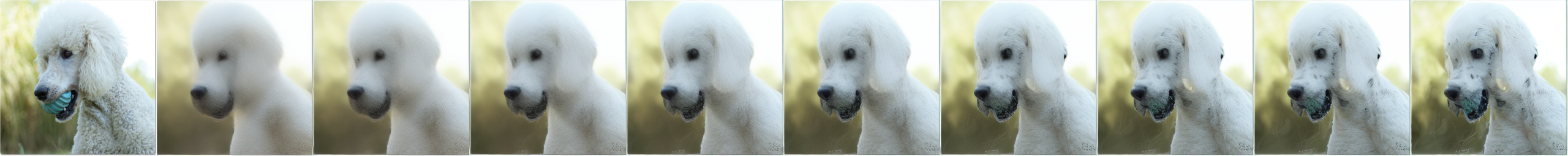
(a) standard poodle $\rightarrow$ dalmatian

(b) golf ball $\rightarrow$ baseball

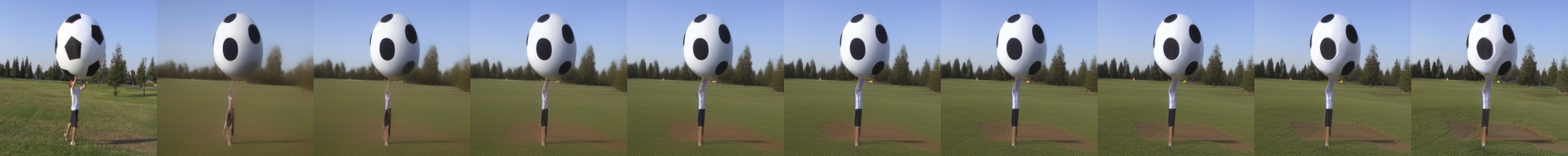
(c) soccer ball $\rightarrow$ golf ball

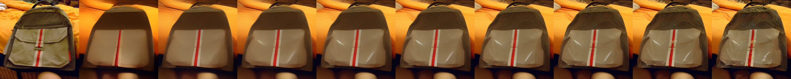
(d) backpack $\rightarrow$ plastic bag

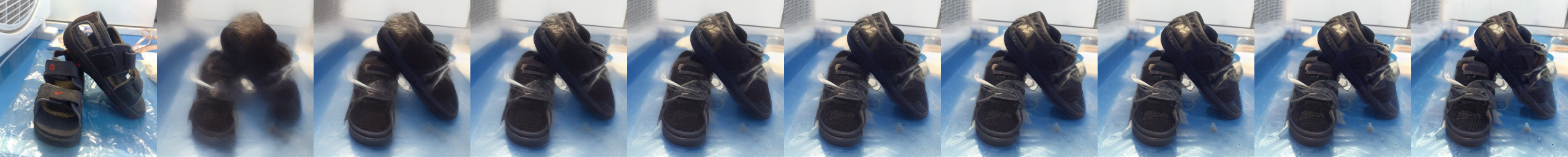
(e) sandal $\rightarrow$ running shoe

Figure 8: Visualization of changes over the course of the counterfactual generation. From left to right: (f)actual image $x^{\mathrm{F}}$, intermediate visualizations (linearly spaced) till final counterfactual $x^{\mathrm{CF}}$.

Appendix G Diversity of the generated counterfactual explanations

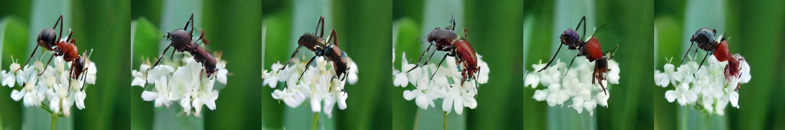
(a) ant $\rightarrow$ ground beetle

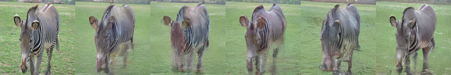
(b) zebra $\rightarrow$ hippopotamus

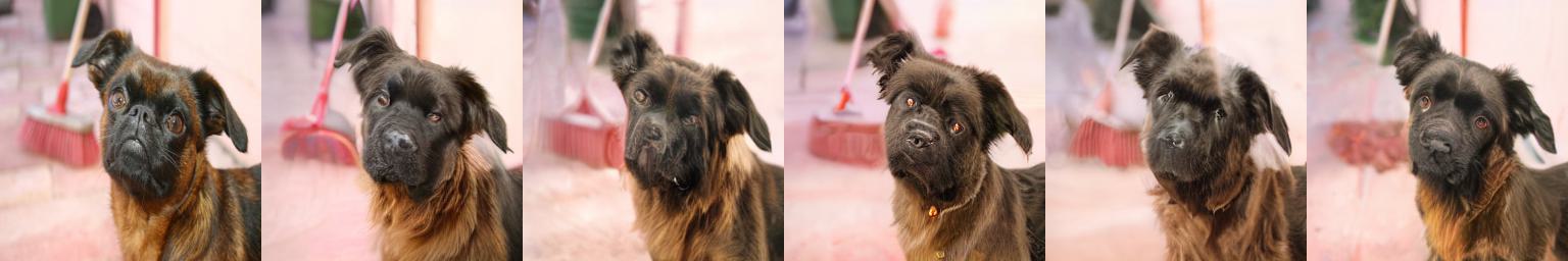
(c) brabancon griffon $\rightarrow$ newfoundland

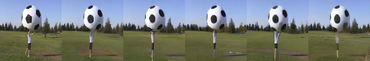
(d) soccer ball $\rightarrow$ golfball

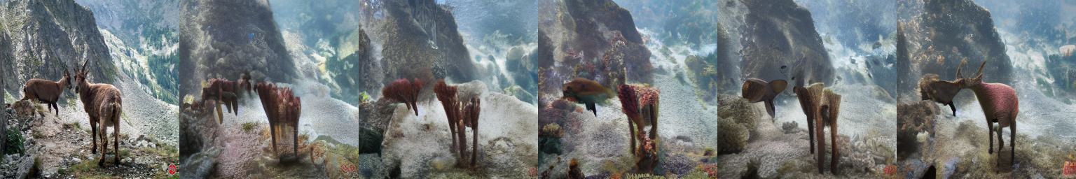
(e) alp $\rightarrow$ coral reef

Figure 9: Qualitative diversity assessment across five different random seeds (0-4) using LDCE-txt on ImageNet (Deng et al., 2009) with ResNet-50 (He et al., 2016). From left to right: original image, counterfactual image generated by LDCE-txt for five different seeds.

Diffusion models by design are capable of generating image distributions. While the used DDIM sampler (Song et al., 2021) is deterministic, we remark that the abduction step (application of forward diffusion onto the (f)actual input $x^{\textrm{F}}$) still introduces stochasticity in our approach, resulting in the generation of diverse counterfactual images. More specifically, Figure 9 shows that the injected noise influences the features that are added to or removed from the (f)actual image at different scales. Therefore, to gain a more comprehensive understanding of the underlying semantics driving the transitions in classifiers’ decisions, we recommend to generate counterfactuals for multiple random seeds.

Appendix H Quantitative results on CelebA HQ

Table 6 provides quantitative comparison to previous methods on CelebA HQ (Lee et al., 2020). We compared to DiVE (Rodriguez et al., 2021), STEEX (Jacob et al., 2022), DiME (Jeanneret et al., 2022), and ACE (Jeanneret et al., 2023) on CelebA HQ (Lee et al., 2020) using a DenseNet-121 (Jacob et al., 2022). Note that in contrast to previous works, LDCE-txt is not specifically trained on a face image distribution and still yields competitive quantitative results. Table 6, Figure 4(a)-(d) as well as Figure 12 demonstrate the ability of LDCE-txt to capture and manipulate distinctive facial features, also showcasing its efficacy in the domain of human faces: LDCE-txt inserts or removes local features such as wrinkles, dimples, and eye bags when moving along the smile and age attributes.

Table 6: Quantitative comparison to previous works using DenseNet-121 on CelebA HQ. All methods except for ours require access to the target classifier’s training data distribution.

Smile
Method	FID ($\downarrow$)	sFID ($\downarrow$)	FVA ($\uparrow$)	FS ($\uparrow$)	MNAC ($\downarrow$)	CD ($\downarrow$)	COUT ($\uparrow$)
DiVE (Rodriguez et al., 2021)	107.0	-	35.7	-	7.41	-	-
STEEX (Jacob et al., 2022)	21.9	-	97.6	-	5.27	-	-
DiME (Jeanneret et al., 2022)	18.1	27.7	96.7	0.6729	2.63	1.82	0.6495
ACE $\ell_{1}$ (Jeanneret et al., 2023)	3.21	20.2	100.0	0.8941	1.56	2.61	0.5496
ACE $\ell_{2}$ (Jeanneret et al., 2023)	6.93	22.0	100.0	0.8440	1.87	2.21	0.5946
LDCE-txt	13.6	25.8	99.1	0.756	2.44	1.68	0.3428
Age
DiVE (Rodriguez et al., 2021)	107.5	-	32.3	-	6.76	-	-
STEEX (Jacob et al., 2022)	26.8	-	96.0	-	5.63	-	-
DiME (Jeanneret et al., 2022)	18.7	27.8	95.0	0.6597	2.10	4.29	0.5615
ACE $\ell_{1}$ (Jeanneret et al., 2023)	5.31	21.7	99.6	0.8085	1.53	5.4	0.3984
ACE $\ell_{2}$ (Jeanneret et al., 2023)	16.4	28.2	99.6	0.7743	1.92	4.21	0.5303
LDCE-txt	14.2	25.6	98.0	0.7319	2.12	4.02	0.3297

Appendix I Additional qualitative examples

Figures 11, 12, 13, and 14 provide additional qualitative examples for ImageNet with ResNet-50, CelebA HQ with DenseNet-121, Oxford Pets with OpenCLIP VIT-B/32, or Oxford Flowers 102 with (frozen) DINO-VIT-S/8 with (trained) linear classifier, respectively. Note that, in contrast to standard image generation, editing or prompt-to-prompt tuning, we are interested in minimal semantically meaningful changes to flip a target classifier’s prediction (and not just generating the best looking image).

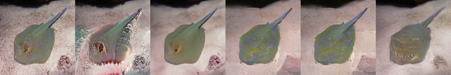
(a) stingray $\rightarrow$ great white shark

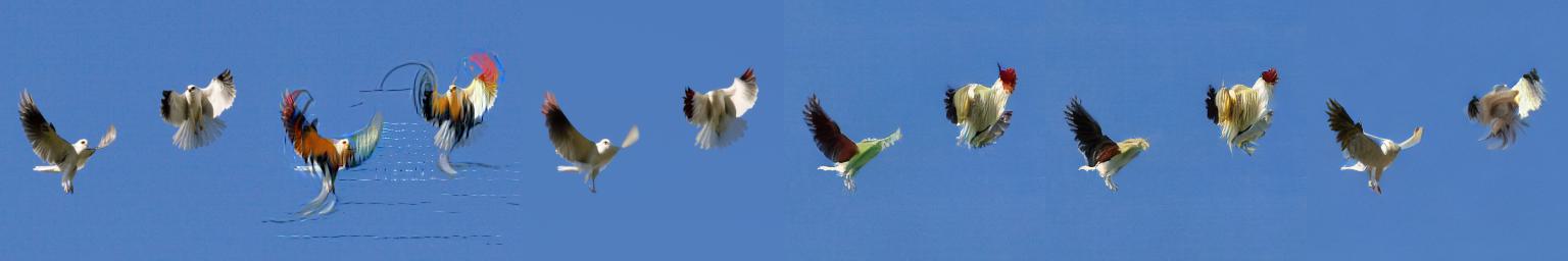
(b) kite $\rightarrow$ rooster

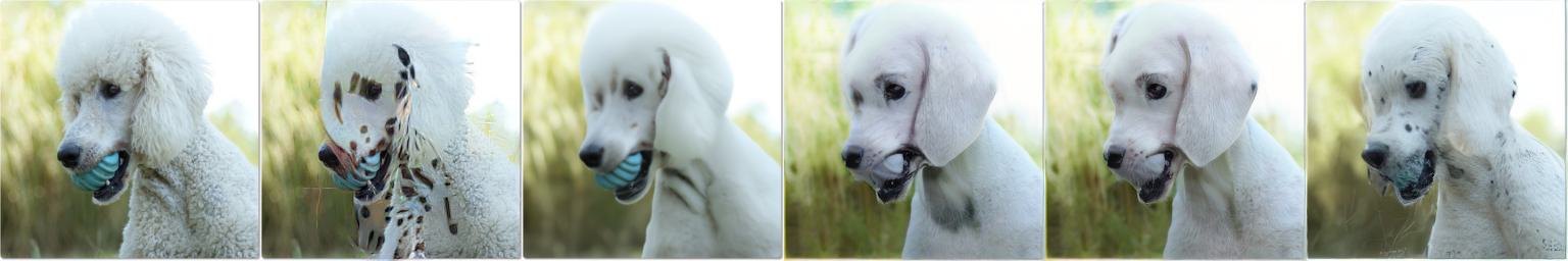
(c) poodle $\rightarrow$ dalmatian

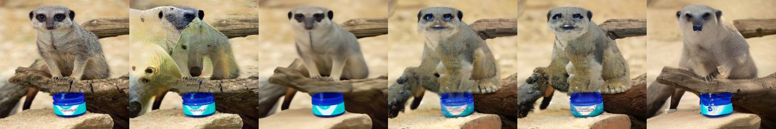
(d) meerkat $\rightarrow$ ice bear

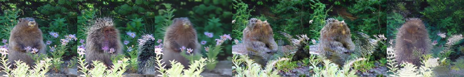
(e) marmot $\rightarrow$ porcupine

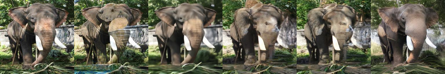
(f) indian elephant $\rightarrow$ african elephant

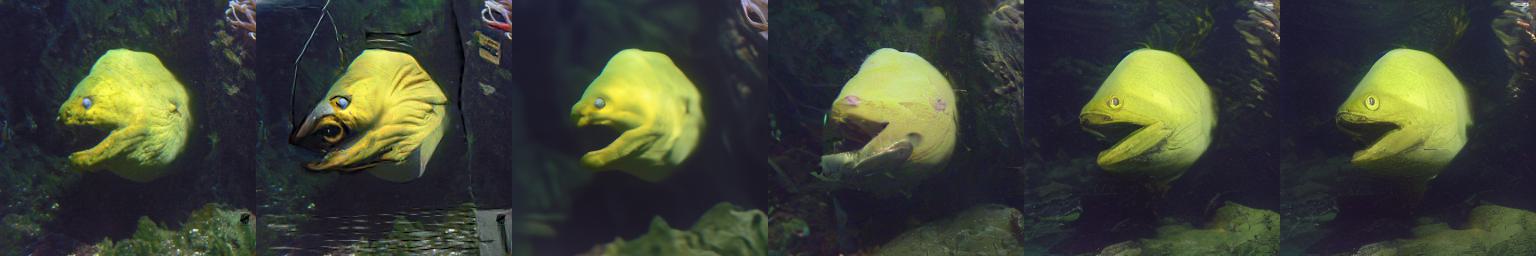
(g) eel $\rightarrow$ coho

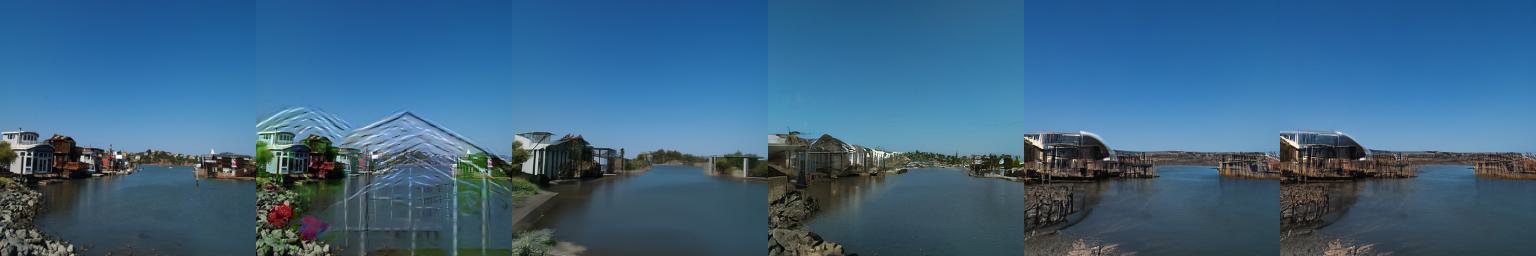
(a) boathouse $\rightarrow$ greenhouse

(b) digital watch $\rightarrow$ wall clock

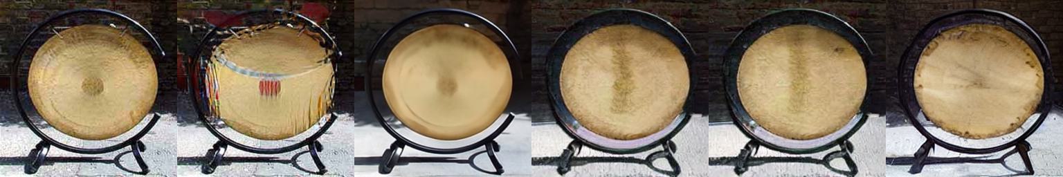
(c) gong $\rightarrow$ drum

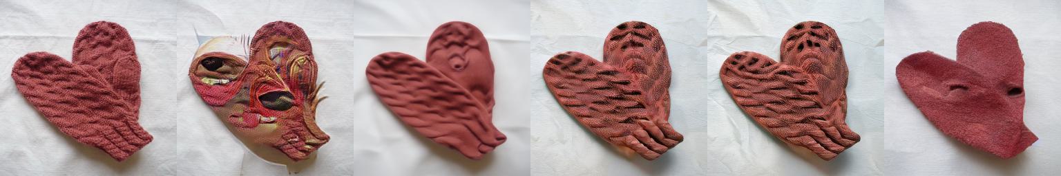
(d) mitten $\rightarrow$ mask

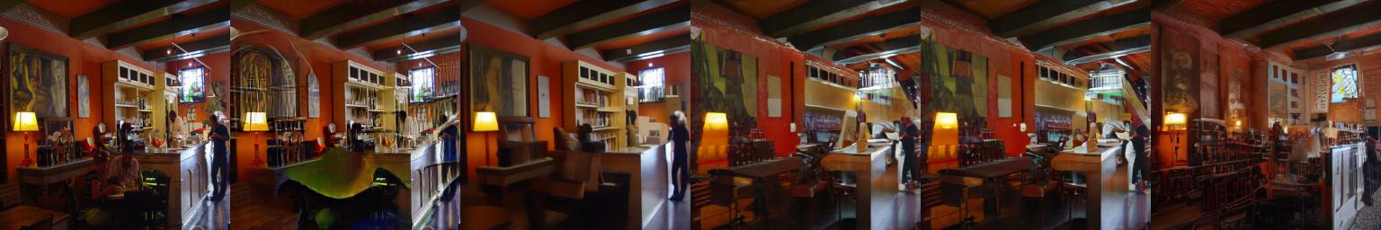
(e) restaurant $\rightarrow$ library

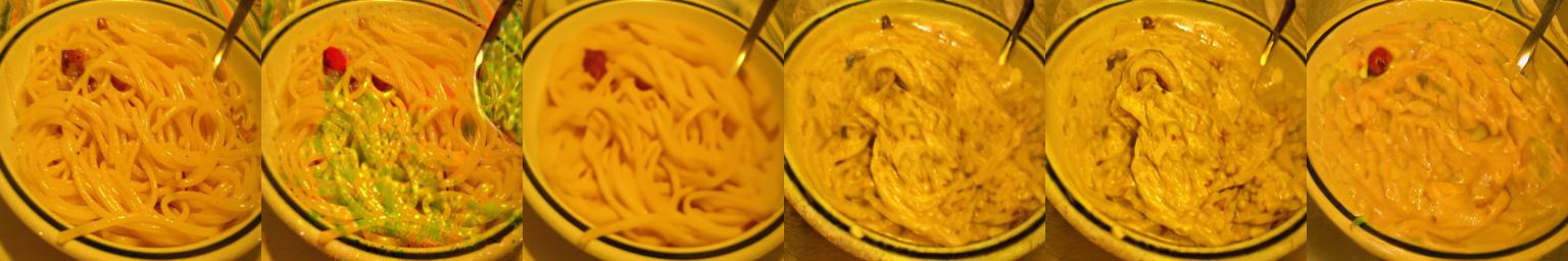
(f) carbonara $\rightarrow$ guacamole

(g) valley $\rightarrow$ cliff

Figure 11: Additional qualitative results for on ImageNet with ResNet-50. From left to right: original image, counterfactual images generated by SVCE (Boreiko et al., 2022), DVCE (Augustin et al., 2022), LDCE-no consensus, LDCE-cls, and LDCE-txt.

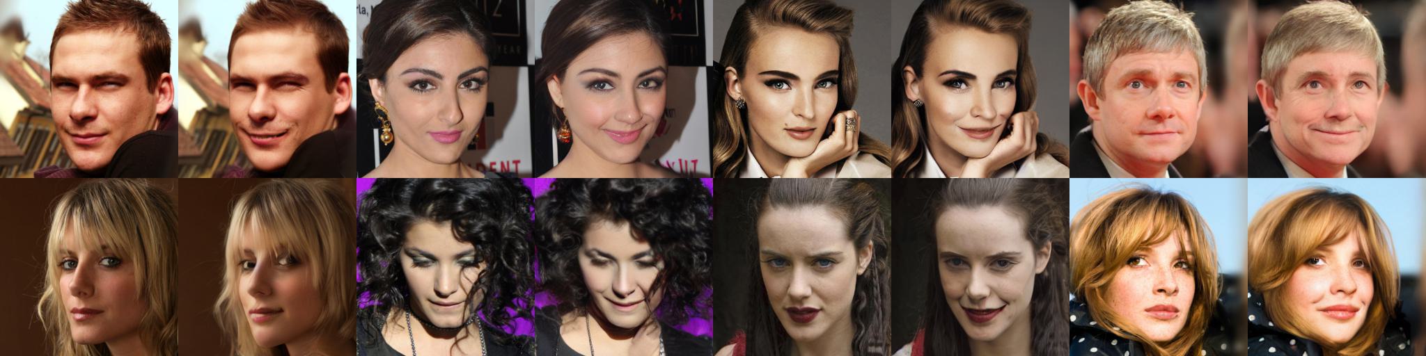
(a) no-smile $\rightarrow$ smile

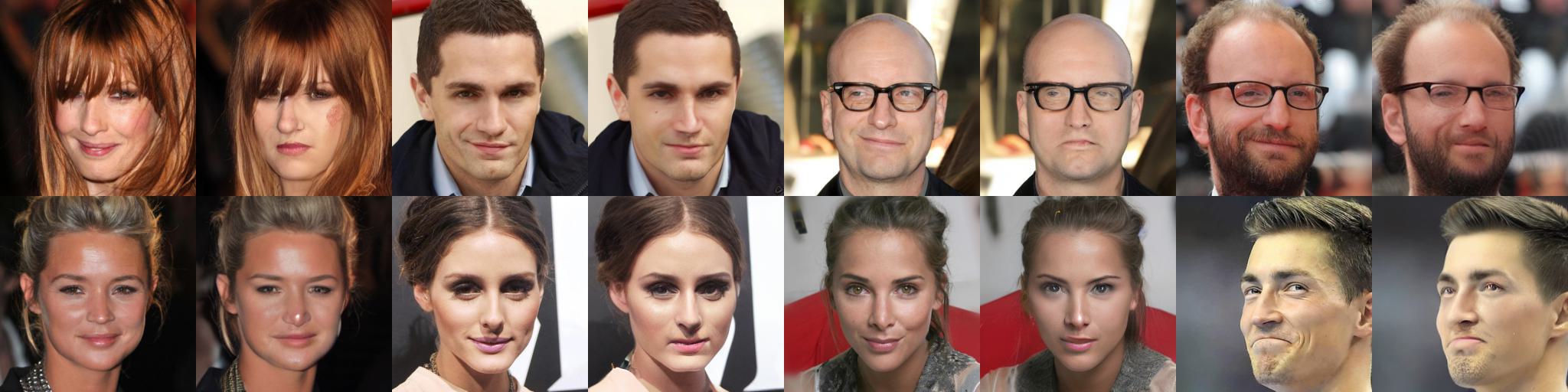
(b) smile $\rightarrow$ no-smile

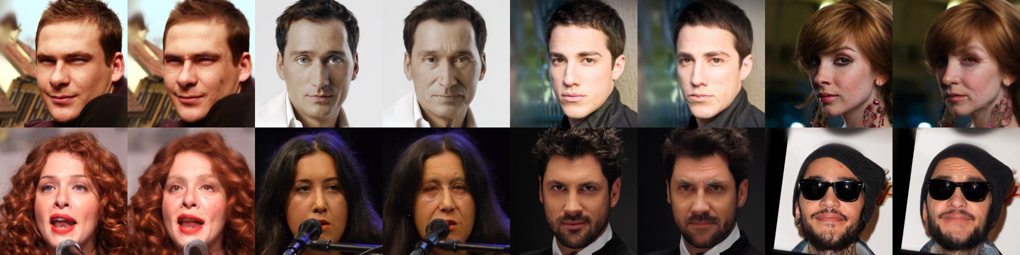
(c) young $\rightarrow$ old

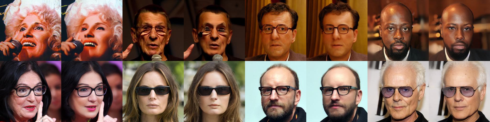
(d) old $\rightarrow$ young

Figure 12: Additional qualitative results for LDCE-txt on CelebA HQ with DenseNet-121. Left: original image. Right: counterfactual image.

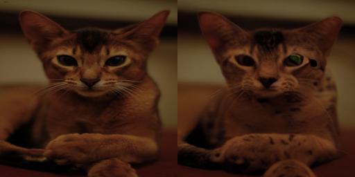
(a) abyssinian $\rightarrow$ egyptian

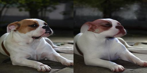
(b) american bulldog $\rightarrow$ sphynx

(c) american pitbull $\rightarrow$ stafford

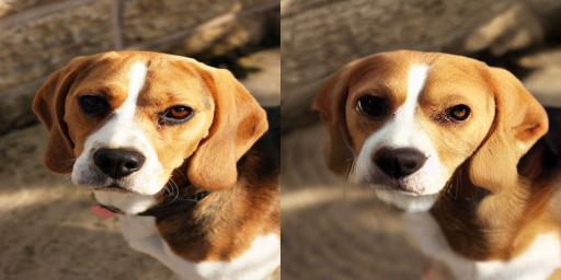
(d) beagle $\rightarrow$ chihuahua

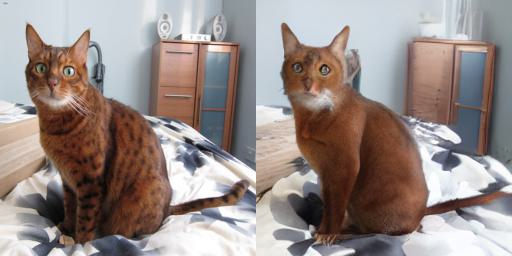
(e) bengal $\rightarrow$ abyssinian

(f) birman $\rightarrow$ siamese

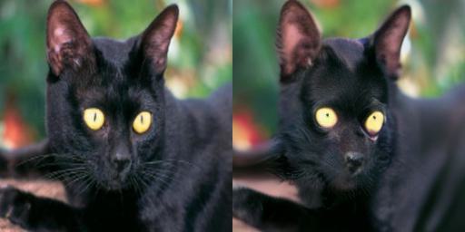
(g) bombay $\rightarrow$ chihuahua

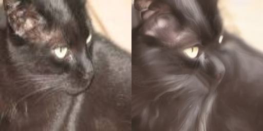
(h) bombay $\rightarrow$ persian

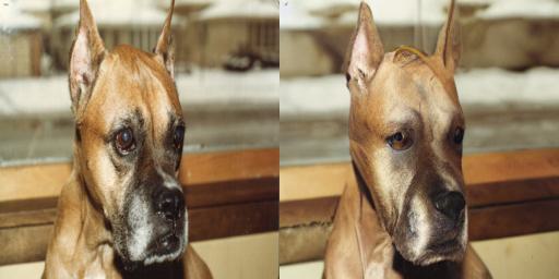
(i) boxer $\rightarrow$ american pitbull

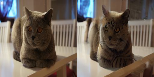
(j) british shorthair $\rightarrow$ bengal

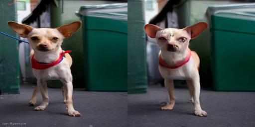
(k) chihuahua $\rightarrow$ sphynx

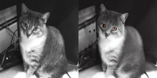
(l) egyptian $\rightarrow$ british shorthair

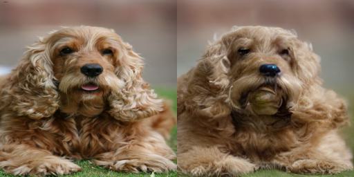
(m) spaniel $\rightarrow$ wheaten

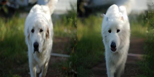
(n) great pyrenees $\rightarrow$ samoyed

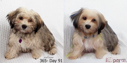
(o) havanese $\rightarrow$ yorkshire

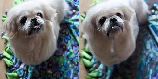
(p) japanese chin $\rightarrow$ boxer

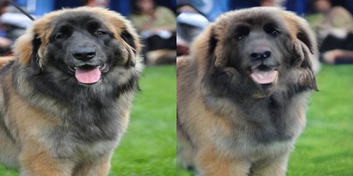
(q) leonberger $\rightarrow$ newfoundland

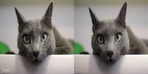
(r) russian blue $\rightarrow$ sphynx

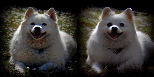
(s) samoyed $\rightarrow$ pomeranian

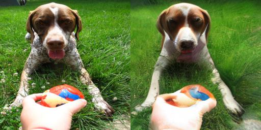
(t) german shorthaired $\rightarrow$ beagle

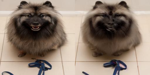
(u) keeshond $\rightarrow$ birman

Figure 13: Additional qualitative results for LDCE-txt on Oxford Pets with OpenCLIP VIT-B/32. Left: original image. Right: counterfactual image.

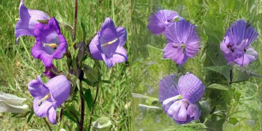
(a) canterbury $\rightarrow$ balloon flower

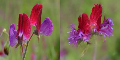
(b) sweet pea $\rightarrow$ bee balm

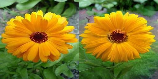
(c) english marigold $\rightarrow$ sunflower

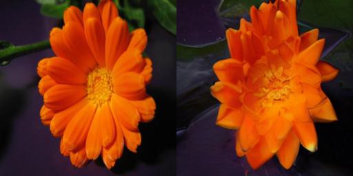
(d) english marigold $\rightarrow$ water lily

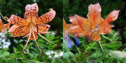
(e) tiger lily $\rightarrow$ stemless gentian

(f) moon orchid $\rightarrow$ spring crocus

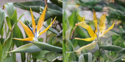
(g) bird of paradise $\rightarrow$ yellow iris

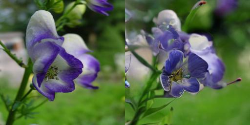
(h) monkshood $\rightarrow$ wallflower

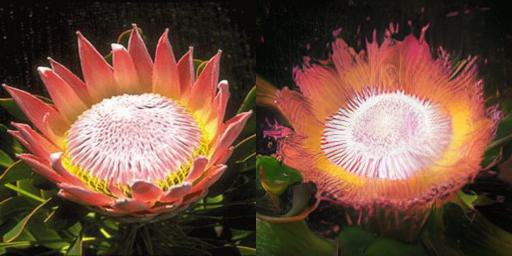
(i) king protea $\rightarrow$ passion flower

(j) preuvian lily $\rightarrow$ watercress

(k) arum lily $\rightarrow$ magnolia

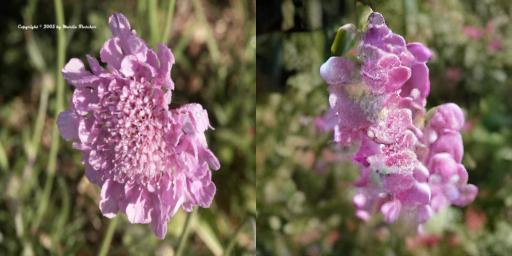
(l) pincushion $\rightarrow$ snapdragon

(m) sweet william $\rightarrow$ petunia

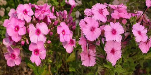
(n) garden phlox $\rightarrow$ sweet william

(o) barbeton daisy $\rightarrow$ gazania

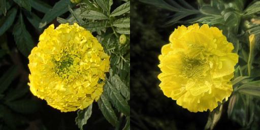
(p) marigold $\rightarrow$ carnation

(q) japanese anemone $\rightarrow$ frangipani

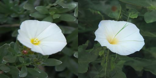
(r) silverbush $\rightarrow$ morning glory

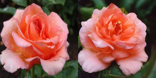
(s) rose $\rightarrow$ camellia

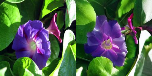
(t) morning glory $\rightarrow$ desert-rose

(u) siam tulip $\rightarrow$ water lily

Figure 14: Additional qualitative results for LDCE-txt on Oxford Flowers 102 with (frozen) DINO-VIT-S/8 with (trained) linear classifier. Left: original image. Right: counterfactual image.

Appendix J Finetuning details

We finetuned the final linear layer of ResNet-50 on the ImageNet training set combined with 25 examples that correspond to the respective model error type for 16 epochs and a batch size of 512. We use stochastic gradient descent with learning rate of 0.1, momentum of 0.9, and weight decay of 0.0005. We used cosine annealing as learning rate scheduler and standard image augmentations (random crop, horizontal flip, and normalization). We evaluated the final model on the holdout test set.

Appendix K Failure modes

In this section, we aim to disclose some observed failure modes of LDCE (specifically LDCE-txt): (i) occasional blurry images (Figure 15(a)), (ii) distorted human bodies and faces (Figure 15(b) and 15(c)), and (iii) a large distance to the counterfactual target class causing difficulties in counterfactual generation (Figure 15(d)). Moreover, we note that these failure modes are further aggravated when multiple instances of the same class (Figure 15(c)) or multiple classes or objects are present in the image (Figure 15(a)).

As discussed in our limitations section (Section 5), we believe that the former cases (i & ii) can mostly be attributed to limitations in the foundation diffusion model, which can potentially be addressed through orthogonal advancements in generative modeling. On the other hand, the latter case (iii) could potentially be overcome by further hyperparameters tuning, e.g., increasing classifier strength $\lambda_{c}$ and decreasing the distance strength $\lambda_{d}$. However, it is important to note that such adjustments may lead to counterfactuals that are farther away from the original instance, thereby possibly violating the desired desiderata of closeness. Another approach would be to increase the number of diffusion steps $T$, but this would result in longer counterfactual generation times. Achieving a balance for these hyperparameters is highly dependent on the specific user requirements and the characteristics of the dataset.

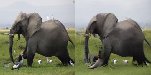
(a) bluriness
african elephant $\rightarrow$ armadillo

(b) distorted bodies
acoustic guitar $\rightarrow$ electric guitar

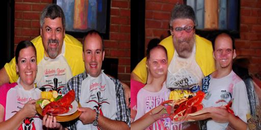
(c) distorted faces
american lobster $\rightarrow$ dungeness crab balm

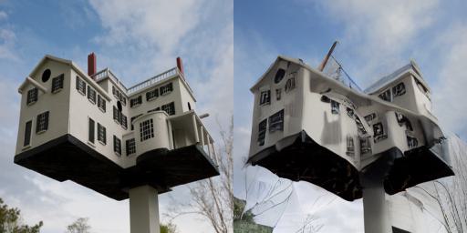
(d) large distance to counterfactual class $y^{\textrm{CF}}$
birdhouse $\rightarrow$ umbrella

Figure 15: Failure modes of LDCE (i.e., LDCE-txt) on ImageNet (Deng et al., 2009) with ResNet-50 (He et al., 2016). Left: original image. Right: counterfactual image.

References

- Akula et al. (2020) Arjun Akula, Shuai Wang, and Song-Chun Zhu. CoCoX: Generating Conceptual and Counterfactual Explanations via Fault-Lines. In AAAI, 2020.
- Arrieta et al. (2020) Alejandro Barredo Arrieta, Natalia Díaz-Rodríguez, Javier Del Ser, Adrien Bennetot, Siham Tabik, Alberto Barbado, Salvador García, Sergio Gil-López, Daniel Molina, Richard Benjamins, et al. Explainable Artificial Intelligence (XAI): Concepts, Taxonomies, Opportunities and Challenges toward Responsible AI. Information Fusion, 2020.
- Augustin et al. (2022) Maximilian Augustin, Valentyn Boreiko, Francesco Croce, and Matthias Hein. Diffusion Visual Counterfactual Explanations. In NeurIPS, 2022.
- Avrahami et al. (2022) Omri Avrahami, Dani Lischinski, and Ohad Fried. Blended diffusion for text-driven editing of natural images. In CVPR, 2022.
- Bach et al. (2015) Sebastian Bach, Alexander Binder, Grégoire Montavon, Frederick Klauschen, Klaus-Robert Müller, and Wojciech Samek. On Pixel-Wise Explanations for Non-Linear Classifier Decisions by Layer-Wise Relevance Propagation. PloS one, 2015.
- Bansal et al. (2023) Arpit Bansal, Hong-Min Chu, Avi Schwarzschild, Soumyadip Sengupta, Micah Goldblum, Jonas Geiping, and Tom Goldstein. Universal guidance for diffusion models. arXiv, 2023.
- Bau et al. (2017) David Bau, Bolei Zhou, Aditya Khosla, Aude Oliva, and Antonio Torralba. Network Dissection: Quantifying Interpretability of Deep Visual Representations. In CVPR, 2017.
- Bianchi et al. (2023) Federico Bianchi, Pratyusha Kalluri, Esin Durmus, Faisal Ladhak, Myra Cheng, Debora Nozza, Tatsunori Hashimoto, Dan Jurafsky, James Zou, and Aylin Caliskan. Easily accessible text-to-image generation amplifies demographic stereotypes at large scale. In FAccT, 2023.
- Böhle et al. (2022) Moritz Böhle, Mario Fritz, and Bernt Schiele. B-cos Networks: Alignment is All We Need for Interpretability. In CVPR, 2022.
- Bolya et al. (2023) Daniel Bolya, Cheng-Yang Fu, Xiaoliang Dai, Peizhao Zhang, Christoph Feichtenhofer, and Judy Hoffman. Token Merging: Your ViT But Faster. In ICLR, 2023.
- Boreiko et al. (2022) Valentyn Boreiko, Maximilian Augustin, Francesco Croce, Philipp Berens, and Matthias Hein. Sparse Visual Counterfactual Explanations in Image Space. In GCPR, 2022.
- Brendel & Bethge (2019) Wieland Brendel and Matthias Bethge. Approximating CNNs with Bag-of-local-Features models works surprisingly well on ImageNet. In ICLR, 2019.
- Brooks et al. (2023) Tim Brooks, Aleksander Holynski, and Alexei A. Efros. InstructPix2Pix: Learning to Follow Image Editing Instructions. In CVPR, 2023.
- Brown et al. (2020) Tom Brown, Benjamin Mann, Nick Ryder, Melanie Subbiah, Jared D Kaplan, Prafulla Dhariwal, Arvind Neelakantan, Pranav Shyam, Girish Sastry, Amanda Askell, et al. Language Models are Few-Shot Learners. In NeurIPS, 2020.
- Cao et al. (2018) Qiong Cao, Li Shen, Weidi Xie, Omkar M Parkhi, and Andrew Zisserman. VGGFace2: A Dataset for recognising faces across pose and age. In IEEE International conference on automatic face & gesture recognition, 2018.
- Caron et al. (2021) Mathilde Caron, Hugo Touvron, Ishan Misra, Hervé Jégou, Julien Mairal, Piotr Bojanowski, and Armand Joulin. Emerging Properties in Self-Supervised Vision Transformers. In ICCV, 2021.
- Chen et al. (2019) Chaofan Chen, Oscar Li, Daniel Tao, Alina Barnett, Cynthia Rudin, and Jonathan K Su. This Looks Like That: Deep Learning for Interpretable Image Recognition. NeurIPS, 2019.
- Chen & He (2021) Xinlei Chen and Kaiming He. Exploring Simple Siamese Representation Learning. In CVPR, 2021.
- Cherti et al. (2022) Mehdi Cherti, Romain Beaumont, Ross Wightman, Mitchell Wortsman, Gabriel Ilharco, Cade Gordon, Christoph Schuhmann, Ludwig Schmidt, and Jenia Jitsev. Reproducible scaling laws for contrastive language-image learning. arXiv, 2022.
- Croce & Hein (2021) Francesco Croce and Matthias Hein. Adversarial Robustness against Multiple and Single -Threat Models via Quick Fine-Tuning of Robust Classifiers. arXiv, 2021.
- Dao et al. (2022) Tri Dao, Dan Fu, Stefano Ermon, Atri Rudra, and Christopher Ré. FLASHATTENTION: Fast and Memory-Efficient Exact Attention with IO-Awareness. In NeurIPS, 2022.
- Deng et al. (2009) Jia Deng, Wei Dong, Richard Socher, Li-Jia Li, Kai Li, and Li Fei-Fei. ImageNet: A Large-Scale Hierarchical Image Database. In CVPR, 2009.
- Dhariwal & Nichol (2021) Prafulla Dhariwal and Alexander Nichol. Diffusion Models Beat GANs on Image Synthesis. In NeurIPS, 2021.
- Dosovitskiy et al. (2021) Alexey Dosovitskiy, Lucas Beyer, Alexander Kolesnikov, Dirk Weissenborn, Xiaohua Zhai, Thomas Unterthiner, Mostafa Dehghani, Matthias Minderer, Georg Heigold, Sylvain Gelly, Jakob Uszkoreit, and Neil Houlsby. An Image is Worth 16x16 Words: Transformers for Image Recognition at Scale. In ICLR, 2021.
- Erhan et al. (2009) Dumitru Erhan, Yoshua Bengio, Aaron Courville, and Pascal Vincent. Visualizing Higher-Layer Features of a Deep Network. University of Montreal, 2009.
- Esser et al. (2021) Patrick Esser, Robin Rombach, and Bjorn Ommer. Taming Transformers for High-Resolution Image Synthesis. In CVPR, 2021.
- Goodfellow et al. (2020) Ian Goodfellow, Jean Pouget-Abadie, Mehdi Mirza, Bing Xu, David Warde-Farley, Sherjil Ozair, Aaron Courville, and Yoshua Bengio. Generative adversarial networks. Communications of the ACM, 2020.
- Goyal et al. (2019) Yash Goyal, Ziyan Wu, Jan Ernst, Dhruv Batra, Devi Parikh, and Stefan Lee. Counterfactual Visual Explanations. In ICML, 2019.
- He et al. (2016) Kaiming He, Xiangyu Zhang, Shaoqing Ren, and Jian Sun. Deep Residual Learning for Image Recognition. In CVPR, 2016.
- Hertz et al. (2023) Amir Hertz, Ron Mokady, Jay Tenenbaum, Kfir Aberman, Yael Pritch, and Daniel Cohen-or. Prompt-to-Prompt Image Editing with Cross-Attention Control. In ICLR, 2023.
- Heusel et al. (2017) Martin Heusel, Hubert Ramsauer, Thomas Unterthiner, Bernhard Nessler, and Sepp Hochreiter. GANs Trained by a Two Time-Scale Update Rule Converge to a Local Nash Equilibrium. NeurIPS, 2017.
- Ho & Salimans (2022) Jonathan Ho and Tim Salimans. Classifier-Free Diffusion Guidance. NeurIPS Workshop, 2022.
- Ho et al. (2020) Jonathan Ho, Ajay Jain, and Pieter Abbeel. Denoising Diffusion Probabilistic Models. In NeurIPS, 2020.
- Huang et al. (2017) Gao Huang, Zhuang Liu, Laurens Van Der Maaten, and Kilian Q Weinberger. Densely Connected Convolutional Networks. In CVPR, 2017.
- Hvilshøj et al. (2021) Frederik Hvilshøj, Alexandros Iosifidis, and Ira Assent. ECINN: Efficient Counterfactuals from Invertible Neural Networks. In BMVC, 2021.
- Jacob et al. (2022) Paul Jacob, Éloi Zablocki, Hédi Ben-Younes, Mickaël Chen, Patrick Pérez, and Matthieu Cord. STEEX: Steering Counterfactual Explanations with Semantics. In ECCV, 2022.
- Jeanneret et al. (2022) Guillaume Jeanneret, Loïc Simon, and Frédéric Jurie. Diffusion Models for Counterfactual Explanations. In ACCV, 2022.
- Jeanneret et al. (2023) Guillaume Jeanneret, Loïc Simon, and Frédéric Jurie. Adversarial Counterfactual Visual Explanations. In CVPR, 2023.
- Jumper et al. (2021) John Jumper, Richard Evans, Alexander Pritzel, Tim Green, Michael Figurnov, Olaf Ronneberger, Kathryn Tunyasuvunakool, Russ Bates, Augustin Žídek, Anna Potapenko, et al. Highly accurate protein structure prediction with AlphaFold. Nature, 2021.
- Khorram & Fuxin (2022) Saeed Khorram and Li Fuxin. Cycle-Consistent Counterfactuals by Latent Transformations. In CVPR, 2022.
- Kim et al. (2018) Been Kim, Martin Wattenberg, Justin Gilmer, Carrie Cai, James Wexler, Fernanda Viegas, et al. Interpretability Beyond Feature Attribution: Quantitative Testing with Concept Activation Vectors (TCAV). In ICML, 2018.
- Kingma & Welling (2014) Diederik P Kingma and Max Welling. Auto-encoding variational bayes. ICLR, 2014.
- Koh et al. (2020) Pang Wei Koh, Thao Nguyen, Yew Siang Tang, Stephen Mussmann, Emma Pierson, Been Kim, and Percy Liang. Concept Bottleneck Models. In ICML, 2020.
- Lang et al. (2021) Oran Lang, Yossi Gandelsman, Michal Yarom, Yoav Wald, Gal Elidan, Avinatan Hassidim, William T Freeman, Phillip Isola, Amir Globerson, Michal Irani, et al. Explaining in Style: Training a GAN to explain a classifier in StyleSpace. In CVPR, 2021.
- Lee et al. (2020) Cheng-Han Lee, Ziwei Liu, Lingyun Wu, and Ping Luo. MaskGAN: Towards Diverse and Interactive Facial Image Manipulation. In CVPR, 2020.
- Loshchilov & Hutter (2019) Ilya Loshchilov and Frank Hutter. Decoupled Weight Decay Regularization. In ICLR, 2019.
- Luccioni et al. (2023) Alexandra Sasha Luccioni, Christopher Akiki, Margaret Mitchell, and Yacine Jernite. Stable Bias: Analyzing Societal Representations in Diffusion Models. In NeurIPS, 2023.
- Lundberg & Lee (2017) Scott M Lundberg and Su-In Lee. A Unified Approach to Interpreting Model Predictions. NeurIPS, 2017.
- Meng et al. (2023) Chenlin Meng, Ruiqi Gao, Diederik P Kingma, Stefano Ermon, Jonathan Ho, and Tim Salimans. On Distillation of Guided Diffusion Models. In CVPR, 2023.
- Miller (1995) George A. Miller. WordNet: a lexical database for English. Communications of the ACM, 1995.
- Nilsback & Zisserman (2008) Maria-Elena Nilsback and Andrew Zisserman. Automated Flower Classification over a Large Number of Classes. In Indian Conference on Computer Vision, Graphics & Image Processing, 2008.
- Olah et al. (2017) Chris Olah, Alexander Mordvintsev, and Ludwig Schubert. Feature Visualization. Distill, 2017.
- Parkhi et al. (2012) Omkar M Parkhi, Andrea Vedaldi, Andrew Zisserman, and CV Jawahar. Cats And Dogs. In CVPR, 2012.
- Pinkey (2023) Justin Pinkey. miniSD. https://huggingface.co/justinpinkney/miniSD, 2023.
- Radford et al. (2021) Alec Radford, Jong Wook Kim, Chris Hallacy, Aditya Ramesh, Gabriel Goh, Sandhini Agarwal, Girish Sastry, Amanda Askell, Pamela Mishkin, Jack Clark, et al. Learning Transferable Visual Models From Natural Language Supervision. In ICML, 2021.
- Rezende & Mohamed (2015) Danilo Rezende and Shakir Mohamed. Variational Inference with Normalizing Flows. In ICML, 2015.
- Rezende et al. (2014) Danilo Jimenez Rezende, Shakir Mohamed, and Daan Wierstra. Stochastic Backpropagation and Approximate Inference in Deep Generative Models. In ICML, 2014.
- Rodriguez et al. (2021) Pau Rodriguez, Massimo Caccia, Alexandre Lacoste, Lee Zamparo, Issam Laradji, Laurent Charlin, and David Vazquez. Beyond Trivial Counterfactual Explanations with Diverse Valuable Explanations. In CVPR, 2021.
- Rombach et al. (2022) Robin Rombach, Andreas Blattmann, Dominik Lorenz, Patrick Esser, and Björn Ommer. High-Resolution Image Synthesis with Latent Diffusion Models. In CVPR, 2022.
- Ronneberger et al. (2015) Olaf Ronneberger, Philipp Fischer, and Thomas Brox. U-Net: Convolutional Networks for Biomedical Image Segmentation. In MICCAI, 2015.
- Salimans & Ho (2022) Tim Salimans and Jonathan Ho. Progressive Distillation for Fast Sampling of Diffusion Models. In ICLR, 2022.
- Samangouei et al. (2018) Pouya Samangouei, Ardavan Saeedi, Liam Nakagawa, and Nathan Silberman. ExplainGAN: Model Explanation via Decision Boundary Crossing Transformations. In ECCV, 2018.
- Sanchez & Tsaftaris (2022) Pedro Sanchez and Sotirios A. Tsaftaris. Diffusion Causal Models for Counterfactual Estimation. In CLeaR, 2022.
- Santurkar et al. (2019) Shibani Santurkar, Andrew Ilyas, Dimitris Tsipras, Logan Engstrom, Brandon Tran, and Aleksander Madry. Image Synthesis with a Single (Robust) Classifier. NeurIPS, 2019.
- Sauer & Geiger (2021) Axel Sauer and Andreas Geiger. Counterfactual Generative Networks. In ICLR, 2021.
- Schuhmann et al. (2021) Christoph Schuhmann, Richard Vencu, Romain Beaumont, Robert Kaczmarczyk, Clayton Mullis, Aarush Katta, Theo Coombes, Jenia Jitsev, and Aran Komatsuzaki. LAION-400M: Open Dataset of CLIP-Filtered 400 Million Image-Text Pairs. arXiv, 2021.
- Selvaraju et al. (2017) Ramprasaath R Selvaraju, Michael Cogswell, Abhishek Das, Ramakrishna Vedantam, Devi Parikh, and Dhruv Batra. Grad-CAM: Visual Explanations from Deep Networks via Gradient-based Localization. In CVPR, 2017.
- Simonyan et al. (2014) Karen Simonyan, Andrea Vedaldi, and Andrew Zisserman. Deep Inside Convolutional Networks: Visualising Image Classification Models and Saliency Maps. ICLR Workshop, 2014.
- Slack et al. (2021) Dylan Slack, Anna Hilgard, Himabindu Lakkaraju, and Sameer Singh. Counterfactual Explanations Can Be Manipulated. NeurIPS, 2021.
- Sohl-Dickstein et al. (2015) Jascha Sohl-Dickstein, Eric Weiss, Niru Maheswaranathan, and Surya Ganguli. Deep Unsupervised Learning using Nonequilibrium Thermodynamics. In ICML, 2015.
- Song et al. (2021) Jiaming Song, Chenlin Meng, and Stefano Ermon. Denoising Diffusion Implicit Models. In ICLR, 2021.
- Song & Ermon (2019) Yang Song and Stefano Ermon. Generative Modeling by Estimating Gradients of the Data Distribution. In NeurIPS, 2019.
- Song et al. (2023) Yang Song, Prafulla Dhariwal, Mark Chen, and Ilya Sutskever. Consistency Models. arXiv, 2023.
- Szegedy et al. (2016) Christian Szegedy, Vincent Vanhoucke, Sergey Ioffe, Jon Shlens, and Zbigniew Wojna. Rethinking the Inception Architecture for Computer Vision. In CVPR, 2016.
- Thiagarajan et al. (2021) Jayaraman Thiagarajan, Vivek Sivaraman Narayanaswamy, Deepta Rajan, Jia Liang, Akshay Chaudhari, and Andreas Spanias. Designing Counterfactual Generators using Deep Model Inversion. In NeurIPS, 2021.
- TorchVision maintainers and contributors (2016) TorchVision maintainers and contributors. TorchVision: PyTorch’s Computer Vision library. https://github.com/pytorch/vision, 2016.
- Van Looveren & Klaise (2021) Arnaud Van Looveren and Janis Klaise. Interpretable Counterfactual Explanations Guided by Prototypes. In ECML PKDD, 2021.
- Vandenhende et al. (2022) Simon Vandenhende, Dhruv Mahajan, Filip Radenovic, and Deepti Ghadiyaram. Making Heads or Tails: Towards Semantically Consistent Visual Counterfactuals. In ECCV, 2022.
- Wachter et al. (2017) Sandra Wachter, Brent Mittelstadt, and Chris Russell. Counterfactual Explanations Without Opening the Black Box: Automated Decisions and the GDPR. Harv. JL & Tech., 2017.
- Wallace et al. (2023) Bram Wallace, Akash Gokul, Stefano Ermon, and Nikhil Naik. End-to-End Diffusion Latent Optimization Improves Classifier Guidance. arXiv, 2023.
- Wang et al. (2021) Pei Wang, Yijun Li, Krishna Kumar Singh, Jingwan Lu, and Nuno Vasconcelos. IMAGINE: Image Synthesis by Image-Guided Model Inversion. In CVPR, 2021.