Kohn-Sham accuracy from orbital-free density functional theory via $\Delta$-machine learning

Abstract

We present a $\Delta$-machine learning model for obtaining Kohn-Sham accuracy from orbital-free density functional theory (DFT) calculations. In particular, we employ a machine learned force field (MLFF) scheme based on the kernel method to capture the difference between Kohn-Sham and orbital-free DFT energies/forces. We implement this model in the context of on-the-fly molecular dynamics simulations, and study its accuracy, performance, and sensitivity to parameters for representative systems. We find that the formalism not only improves the accuracy of Thomas-Fermi-von Weizsäcker (TFW) orbital-free energies and forces by more than two orders of magnitude, but is also more accurate than MLFFs based solely on Kohn-Sham DFT, while being more efficient and less sensitive to model parameters. We apply the framework to study the structure of molten Al_0.88Si_0.12, the results suggesting no aggregation of Si atoms, in agreement with a previous Kohn-Sham study performed at an order of magnitude smaller length and time scales.

I Introduction

Kohn-Sham density functional theory (DFT) Kohn and Sham (1965); Hohenberg and Kohn (1964) is a widely used ab initio method that has a high accuracy to cost ratio relative to other such first principles methods. However, while less expensive than wavefunction-based methods, Kohn-Sham calculations are still associated with significant computational cost. In particular, they scale cubically with the number of atoms/electrons in the system, a consequence of the orthonormality constraint on the Kohn-Sham orbitals, which restricts the length and time scales accessible to such a rigorous quantum mechanical investigation. This bottleneck is particularly severe in molecular dynamics (MD) simulations, where the Kohn-Sham equations may need to be solved thousands or even hundreds of thousands of times to reach time scales relevant to the phenomena of interest Burke (2012).

Orbital-free DFT Lignères and Carter (2005) represents a simplified version of Kohn-Sham DFT in which the orbital-dependent non-interacting kinetic energy functional is replaced by an explicit functional of the electron density. In so doing, the orbitals are removed from the formalism, thereby reducing the problem to the calculation of the electron density alone, in the spirit of the Hohenberg-Kohn theorem Hohenberg and Kohn (1964). This can also be interpreted as replacing the fictitious system of non-interacting fermions with a fictitious system of non-interacting bosons Levy, Perdew, and Sahni (1984); Jiang and Pavanello (2021). The absence of orbitals in orbital-free DFT allows for linear scaling with system size, thereby circumventing the cubic scaling bottleneck inherent in Kohn-Sham DFT. However, an exact kinetic energy functional in terms of the density is currently unknown. Since the pioneering work of Thomas Thomas (1927), Fermi Fermi (1928), and von Weizsäcker Weizsäcker (1935), resulting in the Thomas-Fermi-von Weizsäcker (TFW) functional, the lack of universality has motivated the development of a number of semilocal Constantin, Fabiano, and Della Sala (2019); Luo, Karasiev, and Trickey (2018); Constantin, Fabiano, and Della Sala (2018a); Francisco, Carmona-Espíndola, and Gázquez (2021); Perdew and Constantin (2007); Constantin, Fabiano, and Della Sala (2017), nonlocal Huang and Carter (2010); Constantin, Fabiano, and Della Sala (2018b); Ho, Lignères, and Carter (2008); Karasiev and Trickey (2012); Chacón, Alvarellos, and Tarazona (1985); Mazin (1988); Wang and Teter (1992); Wang, Govind, and Carter (1999); Carling and Carter (2003); Zhou, Ligneres, and Carter (2005); Ho et al. (2007); Huang and Carter (2010); Mazin and Singh (1998); Shao, Mi, and Pavanello (2021); Mi, Genova, and Pavanello (2018); Xu et al. (2022); Shin and Carter (2014), and machine learned Golub and Manzhos (2019); Alghadeer, Al-Aswad, and Alharbi (2021); Fujinami et al. (2020); del Mazo-Sevillano and Hermann (2023); Remme et al. (2023); Ryczko et al. (2022); Kumar et al. (2022); Meyer, Weichselbaum, and Hauser (2020); Snyder et al. (2013) kinetic energy functionals. However, while advances have been significant, kinetic energy functionals remain limited in accuracy and transferability, particularly for complex systems with significant inhomogeneity in bonding. Furthermore, the lack of orbitals prevents the use of state-of-the-art pseudopotentials that are available for Kohn-Sham DFT calculations, which further limits the accuracy of orbital-free DFT. Consequently, orbital-free DFT has been less widely used than Kohn-Sham DFT in practice.

$\Delta$-machine learning represents a powerful method for learning the difference in quantities that can be computed from different levels of theory. The effectiveness of such a strategy relies on the qualitative features in the quantities of interest being captured by the lower level of theory, whereby the differences in the quantities between the two theories are smoother and typically more localized than the quantities (obtained from the higher level of theory) themselves. $\Delta$-machine learning has already proven useful in a number of different schemes, including the development of machine learned force fields (MLFFs) Schleder et al. (2019); Poltavsky and Tkatchenko (2021); Unke et al. (2021) for the difference in energies and/or forces from the following lower level to higher level theories: Kohn-Sham DFT to coupled cluster Bowman et al. (2022); Bogojeski et al. (2020); Nandi et al. (2021); Qu et al. (2021), Hartree-Fock to coupled cluster Zaspel et al. (2019); Ramakrishnan et al. (2015); Qiao et al. (2020), Kohn-Sham DFT to random phase approximation for the correlation energy Liu et al. (2022); Verdi et al. (2023), and force fields to coupled cluster Qu et al. (2022a, b); Yu et al. (2023). However, the use of such a technique for learning the difference between orbital-free and Kohn-Sham DFT has not been studied heretofore.

In this work, we present a $\Delta$-machine learning scheme for obtaining Kohn-Sham accuracy from orbital-free DFT calculations. In particular, we model the difference in Kohn-Sham and orbital-free DFT energies/forces using a kernel method based MLFF scheme. We implement this model within the context of on-the-fly MD simulations, and study its accuracy, performance, and sensitivity to parameters for representative systems. We find that the formalism not only improves the accuracy of TFW orbital-free DFT energies and forces by more than two orders of magnitude, but is also more accurate than MLFFs developed directly for Kohn-Sham DFT, while being more efficient and less sensitive to the model parameters. We apply the framework to study the possibility of Si aggregation in molten Al_0.88Si_0.12.

The remainder of the manuscript is organized as follows. In Section II, we discuss the formulation for the $\Delta$-machine learning model between orbital-free and Kohn-Sham DFT. Next, we study the scheme’s accuracy, performance, and sensitivity to model parameters in Section III, where we also apply it to study the structure of molten Al_0.88Si_0.12. Finally, we provide concluding remarks in Section IV.

II Formulation

II.1 $\Delta$-machine learning model

The error in the energy computed by orbital-free DFT can be defined as:

$$E_{\Delta}=E_{\rm KS}-E_{\rm OF}\,,$$ (1)

where $E_{\rm KS}$ and $E_{\rm OF}$ are the Kohn-Sham and orbital-free electronic ground state energies, respectively. The dependence of these energies on the atomic positions has been suppressed for notational simplicity, a strategy adopted henceforth for all other such quantities. Since the ground state electron density in orbital-free DFT is close to Kohn-Sham DFT Thapa et al. (2023), and the electrostatics have the same formalism in both orbital-free and Kohn-Sham DFT, $E_{\Delta}$ is largely free from long-range effects, and can therefore be assumed to depend on only the local environment. This makes $E_{\Delta}$ particularly well suited for machine learning, as exploited in the MLFF model discussed below.

Given any atomic configuration/structure, we assume that the error in the orbital-free DFT energy can be decomposed as Bartók et al. (2010):

$$E_{\Delta}=\sum_{e=1}^{N_{e}}\sum_{i=1}^{N_{A}^{e}}\epsilon_{i}^{e}=\sum_{e=1}^{N_{e}}\sum_{i=1}^{N_{A}^{e}}\sum_{t=1}^{N_{T}^{e}}\tilde{w}_{t}^{e}k\left(\mathbf{x}_{i}^{e},\tilde{\mathbf{x}}_{t}^{e}\right)$$ (2)

where $\epsilon_{i}^{e}$ are the atomic energies, $e$ is the index that runs over the distinct chemical elements, $i$ is the index that runs over the different atoms for each element type, $N_{e}$ is the total number of elements, and $N_{A}^{e}$ is the total number of atoms of the element indexed by $e$. In addition, $\tilde{w}_{t}^{e}$ are the weights, and $k(\mathbf{x}_{i}^{e},\tilde{\mathbf{x}}_{t}^{e})$ is a kernel that measures the distance between the descriptor vectors $\mathbf{x}_{i}^{e}$ and $\tilde{\mathbf{x}}_{t}^{e}$, the latter belonging to the training dataset for the chemical element indexed by $e$, which has $N_{T}^{e}$ such descriptors. We choose the polynomial kernel Bartók, Kondor, and Csányi (2013):

$$k(\mathbf{x}_{i}^{e},\tilde{\mathbf{x}}_{t}^{e})=\left(\frac{\mathbf{x}_{i}^{e}\cdot\tilde{\mathbf{x}}_{t}^{e}}{|\mathbf{x}_{i}^{e}||\tilde{\mathbf{x}}_{t}^{e}|}\right)^{\xi}\,,$$ (3)

where the exponent $\xi$ is a parameter used to control the sharpness of the kernel. In addition, we employ the Smooth Overlap of Atomic Positions (SOAP) formalism Bartók, Kondor, and Csányi (2013), where the rotationally invariant descriptors correspond to the power spectrum of the coefficients $c_{i}^{e}$:

$$[\mathbf{x}_{i}^{e}]_{n_{1}n_{2}l}^{e_{1}e_{2}}=\sqrt{\frac{8\pi^{2}}{2l+1}}\sum_{m=-l}^{l}c_{i,e_{1},n_{1}lm}^{e}c_{i,e_{2},n_{2}lm}^{e*}\,,$$ (4)

where $e_{1},e_{2}\in\{1,2,\ldots,N_{e}\}$, $n_{1},n_{2}\in\{1,2,\ldots,N_{r}\}$, and $l\in\{0,1,...,L_{\rm max}\}$ are used to index the components of the descriptor, a vector of length $N_{r}^{2}N_{e}^{2}(L_{\rm max}+1)$. The coefficients $c_{i}^{e}$ themselves arise during the basis expansion of the atom density for the atom positioned at $\mathbf{r}_{i}^{e}:=(r_{i_{1}}^{e},r_{i_{2}}^{e},r_{i_{3}}^{e})$:

$$b_{i,\tilde{e}}^{e}\left(\mathbf{r}-\mathbf{r}_{i}^{e}\right)=\sum_{l=0}^{L_{\rm max}}\sum_{m=-l}^{l}\sum_{n=1}^{N_{r}}c_{i,\tilde{e},nlm}^{e}j_{l}(q_{nl}|\mathbf{r}-\mathbf{r}_{i}^{e}|)Y_{lm}(\mathbf{r}-\mathbf{r}_{i}^{e})\,,$$ (5)

where $\tilde{e}\in\{1,...,N_{e}\}$, $N_{r}$ is the number of radial basis functions for each $l$, $L_{\rm max}$ is the maximum value of $l$, $Y_{lm}$ are the spherical harmonics, and $j_{l}$ are the normalized spherical Bessel functions, with $q_{nl}$ chosen such that $j_{l}(q_{nl}R_{\rm cut})=0$, $R_{\rm cut}$ being the region of influence for any atom, i.e., the distance within which the atoms are assumed to contribute to the atom density. Since the chosen basis is complete, it allows for systematic convergence. The atom density itself is calculated as Bartók et al. (2010):

$$b_{i,\tilde{e}}^{e}\left(\mathbf{r}-\mathbf{r}_{i}^{e}\right)=\sum_{j=1}^{N_{A}^{\tilde{e}}}f_{\rm cut}\left(|\mathbf{r}_{j}^{\tilde{e}}-\mathbf{r}_{i}^{e}|\right)g\left(\mathbf{r}-\mathbf{r}_{j}^{\tilde{e}}+\mathbf{r}_{i}^{e}\right)\,,$$ (6)

where $f_{\rm cut}$ is the cosine function Behler and Parrinello (2007), and $g$ is the Gaussian function:

$$g\left(\mathbf{r}-\mathbf{r}_{j}^{\tilde{e}}+\mathbf{r}_{i}^{e}\right)=\frac{1}{\sqrt{2\sigma_{a}^{2}\pi}}\exp\left(-\frac{|\mathbf{r}-\mathbf{r}_{j}^{\tilde{e}}+\mathbf{r}_{i}^{e}|^{2}}{2\sigma_{a}^{2}}\right)\,,$$ (7)

with $\sigma_{a}$ being the standard deviation of the Gaussian. A smaller value of $\sigma_{a}$ is suitable for systems with significant heterogeneity, while a larger value of $\sigma_{a}$ is suitable for systems that are homogeneous. On using the single center expansion of the Gaussian function Kaufmann and Baumeister (1989), the coefficients $c_{i}^{e}$ can be written as Bartók, Kondor, and Csányi (2013); Jinnouchi, Karsai, and Kresse (2019):

$$c_{i,\tilde{e},nlm}^{e}=\sum_{j=1}^{N_{A}^{\tilde{e}}}h_{nl}\left(|\mathbf{r}_{j}^{\tilde{e}}-\mathbf{r}_{i}^{e}|\right)Y_{lm}^{*}\left(\mathbf{r}_{j}^{\tilde{e}}-\mathbf{r}_{i}^{e}\right)\,,$$ (8)

where the function $h_{nl}$ itself takes the form:

$$h_{nl}(r)=C(r)\int_{0}^{R_{\rm cut}}j_{l}(q_{nl}r^{\prime})\exp\left(-\frac{r^{\prime 2}+r^{2}}{2\sigma_{a}^{2}}\right)l_{l}\left(\frac{rr^{\prime}}{\sigma_{a}^{2}}\right)r^{\prime 2}{\rm d}r^{\prime}\,,$$ (9)

with $C(r)=4\pi f_{\rm cut}(r)/\sqrt{2\sigma_{a}^{2}\pi}$, and $l_{l}$ being the modified spherical Bessel function of the first kind.

The above described model for $E_{\Delta}$ also provides access to derivatives with respect to atomic positions. In particular, the first-order derivative of $E_{\Delta}$ with respect to atomic position provides a correction to the force computed by orbital-free DFT:

$$f_{\Delta,j_{\alpha}}^{\tilde{e}} =-\frac{\partial E_{\Delta}}{\partial r_{j_{\alpha}}^{\tilde{e}}}$$

$$=-\sum_{e=1}^{N_{e}}\sum_{i=1}^{N_{A}^{e}}\sum_{t=1}^{N_{T}^{e}}\tilde{w}_{t}^{e}\frac{\partial k\left(\mathbf{x}_{i}^{e},\tilde{\mathbf{x}}_{t}^{e}\right)}{\partial\mathbf{x}_{i}^{e}}\cdot\frac{\partial\mathbf{x}_{i}^{e}}{\partial r_{j_{\alpha}}^{\tilde{e}}}$$

$$=\sum_{e=1}^{N_{e}}\sum_{i=1}^{N_{A}^{e}}\sum_{t=1}^{N_{T}^{e}}\tilde{w}_{t}^{e}\xi k\left(\mathbf{x}_{i}^{e},\tilde{\mathbf{x}}_{t}^{e}\right)\mathbf{z}_{i,t}^{e}\cdot\frac{\partial\mathbf{x}_{i}^{e}}{\partial r_{j_{\alpha}}^{\tilde{e}}}\,,$$ (10)

where

$$\mathbf{z}_{i,t}^{e}=\left(\frac{\mathbf{x}_{i}^{e}}{\mathbf{x}_{i}^{e}\cdot\mathbf{x}_{i}^{e}}-\displaystyle\frac{\tilde{\mathbf{x}}_{t}^{e}}{\mathbf{x}_{i}^{e}\cdot\tilde{\mathbf{x}}_{t}^{e}}\right)\,,$$ (11a)

$$\frac{\partial[\mathbf{x}_{i}^{e}]_{n_{1}n_{2}l}^{e_{1}e_{2}}}{\partial r_{j_{\alpha}}^{\tilde{e}}}=c_{l}\sum_{m=-l}^{l}\left(\frac{\partial c_{i,e_{1},n_{1}lm}^{e}}{\partial r_{j_{\alpha}}^{\tilde{e}}}c_{i,e_{2},n_{2}lm}^{e*}+c_{i,e_{1},n_{1}lm}^{e}\frac{\partial c_{i,e_{2},n_{2}lm}^{e*}}{\partial r_{j_{\alpha}}^{\tilde{e}}}\right)\,.$$ (11b)

Above, $c_{l}=\sqrt{8\pi^{2}/(2l+1)}$, and the derivatives of $c_{i}^{e}$ can be obtained to be:

$$\frac{\partial c_{i,\tilde{e},nlm}^{e}}{\partial r_{j_{\alpha}}^{\tilde{e}}}=\begin{cases}\frac{(r_{j_{\alpha}}^{\tilde{e}}-r_{i_{\alpha}}^{e})}{|\mathbf{r}_{j}^{\tilde{e}}-\mathbf{r}_{i}^{e}|}h_{nl}^{\prime}\left(|\mathbf{r}_{j}^{\tilde{e}}-\mathbf{r}_{i}^{e}|\right)Y_{lm}^{*}\left(\mathbf{r}_{j}^{\tilde{e}}-\mathbf{r}_{i}^{e}\right)\\ +h_{nl}\left(|\mathbf{r}_{j}^{\tilde{e}}-\mathbf{r}_{i}^{e}|\right)\frac{\partial Y_{lm}^{*}\left(\mathbf{r}_{j}^{\tilde{e}}-\mathbf{r}_{i}^{e}\right)}{\partial(r_{j_{\alpha}}^{\tilde{e}}-r_{i_{\alpha}}^{e})},&\text{if }j\neq i,\\ -\sum_{k=1,k\neq i}^{N_{A}^{\tilde{e}}}\frac{\partial c_{i,\tilde{e},nlm}^{e}}{\partial r_{k_{\alpha}}^{\tilde{e}}},&\text{if }j=i,\end{cases}$$ (12)

where $h_{nl}^{\prime}$ denotes the derivative of $h_{nl}$. Similarly, the correction to the stress tensor, which represents the first-order derivative of $E_{\Delta}$ with respect to the strain tensor/deformation gradient, has been presented in Appendix A.

II.2 Training: Bayesian linear regression

The expressions for the energy and atomic forces appearing in Eqs. 2 and 10, respectively, can be written in matrix form as:

$$E_{\Delta}^{s}=\sum_{e=1}^{N_{e}}{\bm{K}}_{E}^{s,e}{\bm{w}}^{e}\,,\,\,\,{\bm{f}}_{\Delta}^{s}=\sum_{e=1}^{N_{e}}{\bm{K}}_{f}^{s,e}{\bm{w}}^{e}\,,\quad s\in\{1,...,N_{st}\}\,,$$ (13)

where $s$ is an index introduced for denoting the configuration/structure, ${\bm{w}}^{e}\in\mathbb{R}^{N_{T}^{e}\times 1}$ is a vector of the weights, ${\bm{K}}_{E}^{s,e}\in\mathbb{R}^{1\times N_{T}^{e}}$ is the covariance matrix for the energy, and ${\bm{K}}_{f}^{s,e}\in\mathbb{R}^{\left(3\sum_{e}N_{A}^{e}\right)\times N_{T}^{e}}$ is the covariance matrix for the forces. For numerical purposes, the energy and forces are dimensionless:

$$E^{s}_{\Delta}:=\frac{E_{\Delta}-\mu_{E}}{\sigma_{E}}\,,\quad{\bm{f}}^{s}_{\Delta}:=\frac{{\bm{f}}_{\Delta}}{\sigma_{f}}\,,$$ (14)

where $\mu_{E}$ and ${\sigma_{E}}$ are the mean and standard deviation of $E^{s}_{\Delta}$, respectively, and ${\sigma_{f}}$ is the standard deviation of ${\bm{f}}^{s}_{\Delta}$, all defined over the different structures.

The model weights ${\bm{w}}^{e}$ need to be determined from the data available for training. To do so, we consider Bayesian linear regression, which involves minimizing the loss function Bishop and Nasrabadi (2006):

$$\mathcal{L}\left({\bm{w}}\right) =\frac{\beta}{2}\left(w_{E}^{2}\left\|{\bm{y}}_{E}-\sum_{e=1}^{N_{e}}{\bm{K}}_{E}^{e}{\bm{w}}^{e}\right\|_{2}^{2}\right.$$

$$+\left.w_{f}^{2}\left\|{\bm{y}}_{f}-\frac{\sigma_{E}}{\sigma_{f}}\sum_{e=1}^{N_{e}}{\bm{K}}_{f}^{e}{\bm{w}}^{e}\right\|^{2}_{2}\right)-\frac{\alpha}{2}\|{\bm{w}}\|_{2}^{2}\,,$$ (15)

where

$${\bm{w}} =\left[{{\bm{w}}^{1}};\,{{\bm{w}}^{2}};\,\ldots;\,\ {{\bm{w}}^{N_{e}}}\right]$$ (16a)

$${\bm{K}}_{E}^{e} =[{{\bm{K}}_{E}^{1,e}};\,\ {{\bm{K}}_{E}^{2,e}};\,\ldots;\,{{\bm{K}}_{E}^{N_{st},e}}]\,,$$ (16b)

$${\bm{K}}_{f}^{e} =[{{\bm{K}}_{f}^{1,e}};\,\ {{\bm{K}}_{f}^{2,e}};\,\ldots;\,{{\bm{K}}_{f}^{N_{st},e}}]\,,$$ (16c)

$${\bm{y}}_{E} =[E^{1}_{\Delta};\,E^{2}_{\Delta};\,\ldots;\,E^{N_{st}}_{\Delta}]\,,$$ (16d)

$${\bm{y}}_{f} =[{{\bm{f}}^{1}_{\Delta}};\,{{\bm{f}}^{2}_{\Delta}};\,\ldots;\,{{\bm{f}}^{N_{st}}_{\Delta}}]\,,$$ (16e)

with the semicolon used as a delimiter between the different rows of the vector/matrix. Above, $\alpha$ and $\beta$ are parameters, while $w_{E}$ and $w_{f}$ are the weighting factors for the errors in the energy and forces, respectively. The optimized weights can then be written as:

$${\bm{w}}=\beta{\bm{C}}_{{\bm{w}}}\left({\bm{K}}_{E}^{\rm T}{\bm{y}}_{E}+{\bm{K}}_{f}^{\rm T}{\bm{y}}_{f}\right)\,,$$ (17)

where

$${\bm{C}}_{{\bm{w}}}=\left(\alpha\mathit{I}+\beta\left({\bm{K}}_{E}^{\rm T}{\bm{K}}_{E}+{\bm{K}}_{f}^{\rm T}{\bm{K}}_{f}\right)\right)^{-1}\,,$$ (18)

with the matrices ${\bm{K}}_{E}\in\mathbb{R}^{N_{st}\times(\sum_{e}^{N_{e}}N_{T}^{e})}$ and ${\bm{K}}_{f}\in\mathbb{R}^{N_{st}(3\sum_{e}^{N_{e}}N_{A}^{e})\times(\sum_{e}^{N_{e}}N_{T}^{e})}$ of the form:

$${\bm{K}}_{E} =\left[w_{E}{{\bm{K}}_{E}^{1}};\,w_{E}{{\bm{K}}_{E}^{2}};\,\ldots;\,w_{E}{{\bm{K}}_{E}^{N_{e}}}\right]\,,$$ (19a)

$${\bm{K}}_{f} =\left[w_{f}\frac{\sigma_{E}}{\sigma_{f}}{{\bm{K}}_{f}^{1}};\,w_{f}\frac{\sigma_{E}}{\sigma_{f}}{{\bm{K}}_{f}^{2}};\,\ldots;\,w_{f}\frac{\sigma_{E}}{\sigma_{f}}{{\bm{K}}_{f}^{N_{e}}}\right]\,.$$ (19b)

These optimized weights can then be used in Eq. 13 to predict the energy and forces for any new structure, after having calculated the structure’s covariance matrices for the energy and forces. The uncertainty in the energy (${\bm{\sigma}}_{{\bm{y}}_{E}}$) and forces (${\bm{\sigma}}_{{\bm{y}}_{f}}$) so calculated can be estimated as:

$${\bm{\sigma}}^{2}_{{\bm{y}}_{E}} ={\rm diag}\left(\frac{1}{\beta}+{\bm{K}}_{E}{\bm{C}}_{{\bm{w}}}{\bm{K}}_{E}^{\rm T}\right)\,,$$ (20a)

$${\bm{\sigma}}^{2}_{{\bm{y}}_{f}} ={\rm diag}\left(\frac{1}{\beta}+{\bm{K}}_{f}{\bm{C}}_{{\bm{w}}}{\bm{K}}_{f}^{\rm T}\right)\,,$$ (20b)

where diag(.) refers to the diagonal of the matrix.

III Results and Discussion

We have implemented the above described $\Delta$-machine learning formalism, henceforth referred to as $\Delta_{\rm OF}$-MLFF, within the SPARC electronic structure code Ghosh and Suryanarayana (2017a, b); Xu et al. (2021); Zhang et al. (2023). In particular, we have developed a framework for on-the-fly MD simulations, as outlined in Fig. 1. In such simulations, after a few initial training MD steps for which Kohn-Sham calculations are performed, the energy and atomic forces are set to those predicted by the $\Delta_{\rm OF}$-MLFF model, except when the uncertainty in the forces so computed is larger than a specified threshold $\sigma_{\rm tol}$, at which point the energy and forces are set to those from a Kohn-Sham calculation, which are then also included into the training dataset. Though the current work is focused on energy and atomic forces, the implementation has the capability to also include the stress tensor as part of the training and prediction. The threshold $\sigma_{\rm tol}$ is made to be adaptive by setting it to the maximum value of ${\bm{\sigma}}_{{\bm{y}}_{f}}$ obtained in the $\Delta_{\rm OF}$-MLFF step that is subsequent to a training step Jinnouchi, Karsai, and Kresse (2019). Though this strategy results in increased number of Kohn-Sham calculations in the beginning of the MD simulation, the frequency of such calculations decreases rapidly, whereby the total number of Kohn-Sham calculations in the total MD simulation is generally lower than for other less stringent $\sigma_{\rm tol}$ choices. To avoid the cubic scaling bottleneck encountered in training, a two-step data selection procedure is employed: for any given configuration, we only add those atoms to the training dataset for which the Bayesian error in forces exceeds $\sigma_{\rm tol}$, and then perform CUR Jinnouchi, Karsai, and Kresse (2019) on the resulting dataset for downsampling Jinnouchi, Karsai, and Kresse (2019); Briganti and Lunghi (2023); Young et al. (2021). Note that the parameters $\alpha$ and $\beta$ are also dynamically updated within each training step, by maximizing the evidence function of Bayesian linear regression Bishop and Nasrabadi (2006).

Figure 1: Outline of on-the-fly MD simulations using $\Delta_{\rm OF}$-MLFF.

To study the sensitivity to parameters, accuracy, and efficiency of the $\Delta_{\rm OF}$-MLFF scheme, we consider the following systems: aluminum (Al) at 300 K, silicon (Si) at 300 K, and molten alloy of aluminum-silicon (Al_0.88Si_0.12) at 1473 K. We consider 108-, 216-, and 500-atom cells of Al, Si, and Al_0.88Si_0.12, respectively. As an application, we also study Si aggregation in Al_0.88Si_0.12. In all instances, we perform isokinetic ensemble (NVK) MD with Gaussian thermostat Minary, Martyna, and Tuckerman (2003) and time steps of 4, 4, and 2 fs for the Al, Si, and Al_0.88Si_0.12 systems, respectively. In the Kohn-Sham calculations, we employ optimized norm-conserving Vanderbilt (ONCV) pseudopotentials Hamann (2013) from the SPMS set Shojaei et al. (2023), and the following exchange-correlation functionals: local density approximation (LDA) Perdew and Zunger (1981) for Al, and the Perdew-Burke-Ernzerhof (PBE) Perdew, Burke, and Ernzerhof (1996) variant of the generalized gradient approximation (GGA) for Si and Al_0.88Si_0.12. In the orbital-free calculations, which are also performed using a real-space formalism Ghosh and Suryanarayana (2016); Suryanarayana and Phanish (2014), we employ the Thomas-Fermi-von Weizsäcker (TFW) kinetic energy functional Werzsticxer (1935) (weight factor $\lambda=1$), LDA exchange-correlation functional, and bulk-derived local pseudopotentials (BLPS) Zhou, Wang, and Carter (2004). Note that we have chosen a rather simple kinetic energy functional, since it suffices for achieving the target accuracy for the MD simulations in this work . Indeed, choosing more sophisticated kinetic energy functionals Constantin, Fabiano, and Della Sala (2018b); Luo, Karasiev, and Trickey (2018); Constantin, Fabiano, and Della Sala (2018a); Francisco, Carmona-Espíndola, and Gázquez (2021); Perdew and Constantin (2007); Constantin, Fabiano, and Della Sala (2017); Tomishima and Yonei (1966); Chacón, Alvarellos, and Tarazona (1985); Mazin (1988); Wang and Teter (1992); Wang, Govind, and Carter (1999); Carling and Carter (2003); Zhou, Ligneres, and Carter (2005); Ho et al. (2007); Huang and Carter (2010); Mazin and Singh (1998); Shao, Mi, and Pavanello (2021); Mi, Genova, and Pavanello (2018); Xu et al. (2022); Shin and Carter (2014) is likely to further increase the accuracy of the $\Delta_{\rm OF}$-MLFF scheme, but will also substantially increase the cost.

In presentation of the results, we compare against orbital-free DFT (OF-DFT) as well as MLFF learnt directly from Kohn-Sham DFT (KS-MLFF), i.e., same scheme used for machine learning $E_{\rm KS}$ and the corresponding atomic forces instead. Indeed, OF-DFT and KS-MLFF can be considered to be the limiting cases of the $\Delta_{\rm OF}$-MLFF scheme. All errors are defined with respect to results obtained from Kohn-Sham DFT (KS-DFT). The energy error is defined to be the magnitude of the difference, and the force error is defined to be the maximum difference (in magnitude) in any force component among all the atoms. The errors are averaged over a sufficient number of MD steps to put statistical errors well below the errors under consideration.

III.1 Sensitivity to parameters

We now study the sensitivity of $\Delta_{\rm OF}$-MLFF to the key parameters inherent to the model: hyperparameters in the machine learning model, and the discretization parameters in the orbital-free and Kohn-Sham calculations that are performed. The focus here is on the atomic force errors, since the qualitative trends for the energy errors are similar, with the values generally being one order of magnitude smaller.

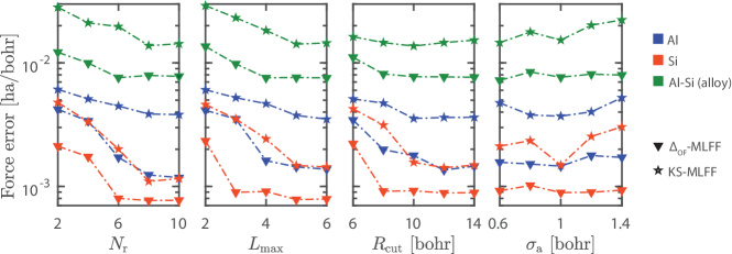
Figure 2: Variation in the force error with respect to the model hyperparameters for the Al, Si, and Al_0.88Si_0.12 systems, averaged over 2000 MD steps.

First, we study the variation in the $\Delta_{\rm OF}$-MLFF errors with respect to the hyperparameters $N_{r}$, $L_{\rm max}$, $R_{\rm max}$, and $\sigma_{a}$, the results so obtained are presented and compared with KS-MLFF in Fig. 2. The Kohn-Sham calculations employ $\Gamma$-point for Brillouin zone integration. Both orbital-free and Kohn-Sham calculations employ mesh sizes of $0.35$, $0.35$, and $0.32$ bohr for the Al, Si, and Al_0.88Si_0.12 systems, respectively, which translates to the energy and forces being converged to within $10^{-4}$ ha/bohr and $10^{-5}$ ha/atom, respectively. We observe that $\Delta_{\rm OF}$-MLFF has consistently smaller errors relative to KS-MLFF. Furthermore, the errors in $\Delta_{\rm OF}$-MLFF have significantly smaller variation with respect to $\sigma_{a}$, and saturate more rapidly with respect to the other hyperparameters, leading to more efficient MLFF training/prediction as well as improved robustness and efficiency with respect to hyperparameter optimization. For the remainder of this work, we select the following hyperparameter values for $\Delta_{\rm OF}$-MLFF: $\{R_{\rm cut},N_{r},L_{\rm max},\sigma_{a}\}=\{8,8,3,1\}$, $\{8,6,4,1\}$, and $\{8,6,4,1\}$ for the Al, Si, and Al_0.88Si_0.12 systems, respectively. The corresponding values for KS-MLFF are $\{10,8,6,1\}$, $\{10,8,5,1\}$, and $\{10,8,5,1\}$, respectively. The values have been chosen such that larger values of $R_{\rm cut}$, $N_{r}$, and $L_{\rm max}$, or different values of $\sigma_{a}$, do not provide any noticeable increase in the accuracy.

Figure 3: Variation in the force error with mesh size for the Al, Si, and Al_0.88Si_0.12 systems, averaged over 1000 MD steps.

Next, we study the variation in the $\Delta_{\rm OF}$-MLFF force errors with mesh size, the results so obtained are presented and compared with OF-DFT and KS-MLFF in Fig. 3. The Kohn-Sham calculations again employ $\Gamma$-point for Brillouin zone integration. We observe that the $\Delta$-MLFF errors are not only significantly smaller than KS-MLFF errors for any given mesh size, but are also less sensitive, suggesting that a coarser grid can be used for $\Delta_{\rm OF}$-MLFF relative to KS-MLFF. In addition, the OF-DFT errors are insensitive to the mesh size, suggesting that the error is completely dominated by the physical error in OF-DFT. The physical error in $\Delta_{\rm OF}$-MLFF appears to be smaller than KS-MLFF, both being significantly lower than OF-DFT, as confirmed below.

Finally, we study the variation in the $\Delta_{\rm OF}$-MLFF force errors with number of Monkhorst-Pack wavevectors at which Brillouin zone integration is performed in KS-DFT, i.e., k-points. The results so obtained are presented and compared with OF-DFT and KS-MLFF in Fig. 4. As before, both orbital-free and Kohn-Sham calculations employ mesh sizes of $0.35$, $0.35$, and $0.32$ bohr for the Al, Si, and Al_0.88Si_0.12 systems, respectively, which translates to the energy and forces being converged to within $10^{-4}$ ha/bohr and $10^{-5}$ ha/atom, respectively. We observe that the $\Delta$-MLFF errors are not only significantly smaller than KS-MLFF errors for any given number of k-points, but are also less sensitive, suggesting that a coarser k-point grid can be used in $\Delta_{\rm OF}$-MLFF relative to KS-MLFF. In addition, the OF-DFT errors are insensitive to the number of k-points used in KS-DFT, confirming that the error is completely dominated by the physical error in OF-DFT. The physical error in $\Delta_{\rm OF}$-MLFF is confirmed to be smaller than KS-MLFF, both being significantly lower than OF-DFT.

Figure 4: Variation in the force error with number of k-points for the Al, Si, and Al_0.88Si_0.12 systems, averaged over 1000 MD steps.

III.2 Accuracy

We now study the accuracy of the $\Delta_{\rm OF}$-MLFF scheme. To do so, we choose orbital-free and Kohn-Sham parameters, including the mesh size and number of k-points, to be such that the energy and atomic forces are converged to within $10^{-5}$ ha/atom and $10^{-4}$ ha/bohr, respectively. This translates to mesh sizes of 0.35, 0.35, and 0.32 bohr for the Al, Si, and Al_0.88Si_0.12 systems, respectively. The corresponding k-point grids are $5\times 5\times 5$, $2\times 2\times 2$, and $3\times 3\times 3$, respectively. We present the results so obtained in Table 1 and compare it with those obtained by OF-DFT as well as KS-MLFF. We observe that $\Delta_{\rm OF}$-MLFF reduces the OF-DFT energy and force errors by more than two orders of magnitude, bringing it close to the accuracy typically desired in KS-DFT MD simulations. In so doing, it is also more accurate than KS-MLFF, by $\sim$ 50%, 50%, and 20% in the energy, and by 35%, 35%, and 30% in the forces, for the Al, Si, and Al_0.88Si_0.12 systems, respectively. Note that the accuracy of both $\Delta_{\rm OF}$-MLFF and KS-MLFF is significantly lower for liquid Al_0.88Si_0.12 compared to solid Al and Si. This can be attributed to the larger configurational space and higher forces in the liquid system. Indeed, the relative accuracy in energy and atomic forces is comparable for all three systems.

Material system	Energy error [ha/atom] ($\times 10^{-5}$)			Force error [ha/bohr] ($\times 10^{-4}$)
	$\Delta_{\rm OF}$-MLFF	OF-DFT	KS-MLFF	$\Delta_{\rm OF}$-MLFF	OF-DFT	KS-MLFF
Al	$3.1$	$776.2$	$6.2$	$5.1$	$170.2$	$7.9$
Si	$2.8$	$726.7$	$5.9$	$4.2$	$192.1$	$6.3$
Al0.88Si0.12	$6.9$	$2651.3$	$8.5$	$61.3$	$735.9$	$88.2$

Table 1: Energy and force errors in $\Delta_{\rm OF}$-MLFF, OF-DFT, and KS-MLFF, averaged over 1000 MD steps.

The orders of magnitude improvement of $\Delta_{\rm OF}$-MLFF over OF-DFT is not surprising, given the rather primitive local/semilocal nature of the TFW kinetic energy functional. In particular, even though the electron density from TFW OF-DFT is found to be close to KS-DFT, the energies and consequently the forces are found to be substantially different Thapa et al. (2023). The use of more sophisticated kinetic energy functionals Huang and Carter (2010); Constantin, Fabiano, and Della Sala (2018b, 2019); Ho, Lignères, and Carter (2008); Karasiev and Trickey (2012) is likely to increase the accuracy of not only OF-DFT, but also $\Delta_{\rm OF}$-MLFF. The ability of the $\Delta_{\rm OF}$-MLFF scheme to achieve higher accuracy than KS-MLFF can be attributed in part to the smoother and more localized nature of $E_{\Delta}$ relative to $E_{\rm KS}$, which makes it more amenable to machine learning. Indeed, the use of more advanced kinetic energy functionals in the orbital-free calculations is likely to widen the gap. Notably, the cancellation of long range electrostatic effects in $E_{\Delta}$ is likely to make $\Delta_{\rm OF}$-MLFF significantly more accurate than KS-MLFF for polar systems. Such systems have not been considered here due to the paucity of accurate and transferable pseudopotentials in OF-DFT.

III.3 Performance

We now study the performance of the $\Delta_{\rm OF}$-MLFF scheme. To do so, we choose all parameters, including mesh size, k-points, and hyperparameters, to be such that the atomic forces in the $\Delta_{\rm OF}$-MLFF scheme are accurate to within $2\times 10^{-3}$, $2\times 10^{-3}$, and $10^{-2}$ ha/bohr for the Al, Si, and Al_0.88Si_0.12 systems, respectively. To facilitate comparison, the mesh sizes and number of k-points in KS-MLFF are also chosen to be such that they provide the aforementioned accuracy in the forces, i.e., same accuracy as $\Delta_{\rm OF}$-MLFF. Note that we do not compare against OF-DFT here since it is not able to achieve this desired accuracy. In fact, the errors in OF-DFT are more than an order of magnitude larger than the accuracy targeted here, as shown in the previous subsection.

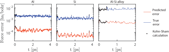
Figure 5: Variation of the true and predicted force error in $\Delta_{\rm OF}$-MLFF for a MD simulation of 1000 steps. The steps where Kohn-Sham calculations have been performed are also indicated.

We present the results so obtained in Table 2, which also contains the mesh sizes and number of k-points chosen for each scheme. We observe that both $\Delta_{\rm OF}$-MLFF and KS-MLFF perform Kohn-Sham calculations on only $\sim$1% of the steps in the MD simulation containing a total of 10,000 steps, with the number of such calculations in $\Delta_{\rm OF}$-MLFF being lower than KS-MLFF by $\sim$ 25%, 25%, and 15% for the Al, Si, and Al_0.88Si_0.12 systems, respectively. Indeed, most of the the Kohn-Sham calculations are performed in the beginning of the MD simulation, with lowering frequency as the simulation progresses, as can be seen in Fig. 5. We also observe that even though the $\Delta_{\rm OF}$-MLFF scheme requires an orbital-free calculation to be performed in each MD step, the overall time is still significantly lower than KS-MLFF, being $\sim$1.5x, $\sim$1.05x, and $\sim$ 3.15x faster for the Al, Si, and Al_0.88Si_0.12 systems, respectively. This is because the computational expense is primarily determined by the cost of the Kohn-Sham calculations, for which the ability to use coarser real space and k-point grids in $\Delta_{\rm OF}$-MLFF, as well as the need to perform fewer such calculations relative to KS-MLFF, can provide substantial savings. This becomes especially true as the system size increases, due to the cubic scaling nature of Kohn-Sham calculations relative to the linear scaling nature of orbital-free and MLFF calculations. Note that there is significant scope of improvement in the current OF-DFT implementation, including the use of preconditioners, which is likely to further increase the efficiency of the $\Delta_{\rm OF}$-MLFF scheme. Also note that though the predicted error and the true error can differ by around an order of magnitude (Fig. 5), they are well-correlated, the correlation coefficient being $0.65-0.70$, which is similar to that obtained for the KS-MLFF scheme, both here and in literature Jinnouchi, Karsai, and Kresse (2019). Indeed, this difference between the true and predicted error is system dependent and is therefore not known apriori.

Material system	Method	Discretization parameters		# Kohn-Sham steps performed	Time [CPU hours]
		Mesh size	k-point		Kohn-Sham	MLFF	Orbital-free	Total
		[bohr]	grid
Al	$\Delta_{\rm OF}$-MLFF	0.55	$1\times 1\times 1$	66	2.9	18.1	34.2	55.2
	KS-MLFF	0.35	$2\times 2\times 2$	87	63.2	18.4	-	81.6
Si	$\Delta_{\rm OF}$-MLFF	0.55	$1\times 1\times 1$	55	5.5	32.1	62.2	99.8
	KS-MLFF	0.35	$1\times 1\times 1$	76	61.4	42.7	-	104.1
Al0.88Si0.12	$\Delta_{\rm OF}$-MLFF	0.55	$1\times 1\times 1$	89	45.3	152.1	196.1	393.5
	KS-MLFF	0.35	$2\times 2\times 2$	103	1079.2	156.1	-	1235.3

Table 2: Computational time of $\Delta_{\rm OF}$-MLFF and KS-MLFF for a MD simulation of 10,000 steps.

III.4 Application: structure of molten Al_0.88Si_0.12

We now apply the $\Delta_{\rm OF}$-MLFF scheme to study the possibility of Si aggregation in the molten Al_0.88Si_0.12 alloy. Experiments have measured a spatial variation in the density of molten Al_0.88Si_0.12, which has been attributed to Si aggregation and the formation of Si clusters within the alloy Dahlborg et al. (2007). This was however contradicted by KS-DFT simulations Khoo et al. (2011), though the relatively small length (500-atom cell) and time scales (10 ps) associated with these simulations has been suggested as a possible reason for the disagreement, which provides the motivation for the current study.

First, we verify the scheme’s accuracy for this application by calculating the pair distribution functions (PDFs) for the alloy, and comparing it with those obtained by OF-DFT and KS-DFT. As before, we consider a 500-atom cell at a temperature of 1473 K, $\Gamma-$point Brillouin zone integration in Kohn-Sham calculations, 12-th order finite-differences with mesh size of 0.55 bohr, which provides an accuracy of $10^{-4}$ ha/atom and $10^{-2}$ ha/bohr in the energy and atomic forces, respectively, in both orbital-free and Kohn-Sham calculations, and NVK MD simulations with Gaussian thermostat and a timestep of 2 fs, for a total of 10,000 steps. Note that PDFs are well-converged with respect to all the parameters in the orbital-free and Kohn-Sham calculations, the results so obtained presented in Fig. 6. We observe that the PDFs from $\Delta_{\rm OF}$-MLFF are nearly indistinguishable to those from KS-DFT, while those from OF-DFT are significantly different, which demonstrates the substantially increased accuracy of the $\Delta_{\rm OF}$-MLFF scheme relative to OF-DFT. Note that the PDFs obtained here are also in good agreement with those in literature obtained using KS-DFT Khoo et al. (2011), further verifying the accuracy of the simulations.

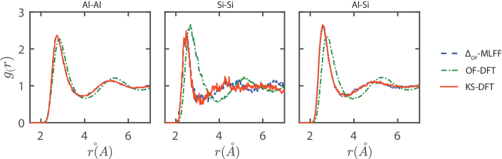
Figure 6: Pair distribution functions for the molten Al_0.88Si_0.12 alloy at 1473 K, as computed by $\Delta_{\rm OF}$-MLFF, OF-DFT, and KS-DFT.

Next, we perform the MD simulation with a 5000-atom cell for 50,000 steps, i.e., a total time of 100 ps. All parameters are identical to those used for the calculation of the PDFs. The $\Delta$-MLFF model trained during the 500-atom MD simulation is used as the initial model for the 5000-atom simulation, a strategy referred to as transfer learning. In so doing, the complete simulation requires only six Kohn-Sham calculations, thereby providing significant computational savings. To examine the aggregation of Si atoms, we analyze the distribution of the Al and Si neighbors, as depicted in Fig. 7. We observe that the ratio of Al to Si nearest neighbors aligns closely with that expected from a random distribution, indicating a homogeneous chemical mixing in the system. In addition, the most common coordination for the Si atoms is nine Al atoms and zero Si atoms in the nearest neighbor shell. Notably, there are very few Si atoms with more than two Si nearest neighbors and virtually none with more than four. Though these results correspond to 1473 K, we have verified that the qualitative features remain unchanged at 1000 and 1200 K. Indeed, the results are nearly identical to those for the 500-atom cell, which are also in very good agreement with the aforementioned KS-DFT investigation Khoo et al. (2011). Therefore, the current results do not support the hypothesis of silicon aggregation Dahlborg et al. (2007), in agreement with previous KS-DFT Khoo et al. (2011) and force field simulations Huang et al. (2019).

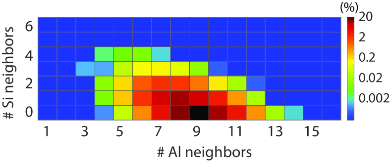
Figure 7: Distribution of Al and Si neighbors for Si atoms in molten Al_0.88Si_0.12 at 1473 K, as computed using $\Delta_{\rm OF}$-MLFF.

IV Concluding remarks

In this work, we have presented a $\Delta$-machine learning model for obtaining Kohn-Sham accuracy from orbital-free DFT calculations. In particular, a MLFF scheme based on the kernel method, with SOAP descriptors and weights determined though Bayesian linear regression, has been employed for capturing the differences between the Kohn-Sham and orbital-free DFT energies/forces, the resulting formalism referred to as $\Delta_{\rm OF}$-MLFF. We have implemented $\Delta_{\rm OF}$-MLFF in the context of on-the-fly MD simulations, whose accuracy, performance, and sensitivity to parameters has been studied for the aluminum, silicon, and molten aluminum silicon alloy (Al_0.88Si_0.12) systems. We have found that $\Delta_{\rm OF}$-MLFF is not only more accurate than TFW orbital-free DFT by more than two orders of magnitude, but is also more accurate than MLFFs generated solely from Kohn-Sham DFT, while being more efficient and less sensitive to the model parameters. We have applied the $\Delta_{\rm OF}$-MLFF scheme to study the structure of molten Al_0.88Si_0.12, for which we have found no evidence of Si aggregation, in agreement with a previous Kohn-Sham DFT investigation performed at an order of magnitude smaller length and time scales.

The use of more advanced kinetic energy functionals for the orbital-free calculations in the $\Delta_{\rm OF}$-MLFF scheme is likely to further increase its accuracy. In this context, the choice/development of functionals that have the best balance between accuracy and computational cost is a worthy subject for future research. The implementation of $\Delta_{\rm OF}$-MLFF on GPUs is likely to significantly bring down the solution times, as demonstrated recently for the associated Kohn-Sham calculations Sharma et al. (2023), making it another subject worthy for future research. From a MLFF perspective, the current findings suggest that orbital-free DFT and other fast physical approximations can provide a valuable complement to machine learning techniques, indicating that renewed focus on improving the speed, accuracy, and general applicability of orbital-free DFT is warranted.

Appendix A Stress tensor in the $\Delta$-machine learning model

In the $\Delta$-machine learning model, the correction to the stress tensor computed by orbital-free DFT takes the form:

$$\sigma_{\Delta,\lambda\mu} =\frac{1}{V}\left.\frac{\partial E_{\Delta}^{F}}{\partial F_{\lambda\mu}}\right|_{\mathbf{F}=\mathbf{I}}\,,$$

$$=-\frac{1}{V}\sum_{e=1}^{N_{e}}\sum_{i=1}^{N_{A}^{e}}\sum_{t=1}^{N_{T}^{e}}\tilde{w}_{t}^{e}\xi k\left(\mathbf{x}_{i}^{e},\tilde{\mathbf{x}}_{t}^{e}\right)\mathbf{z}_{i,t}^{e}\cdot\left.\frac{\partial{\mathbf{x}_{i}^{e}}^{F}}{\partial F_{\lambda\mu}}\right|_{\mathbf{F}=\mathbf{I}}\,.$$ (21)

where

$$\left.\frac{\partial[{\mathbf{x}_{i}^{e}}^{F}]_{n_{1}n_{2}l}^{e_{1}e_{2}}}{\partial F_{\lambda\mu}}\right|_{\mathbf{F}=\mathbf{I}} =c_{l}\sum_{m=-l}^{l}\left(\frac{\partial{c^{e}}^{F}_{i,e_{1},n_{1}lm}}{\partial F_{\lambda\mu}}{c^{e*}}^{F}_{i,e_{2},n_{2}lm}\right.$$

$$+\left.\left.{c^{e}}^{F}_{i,e_{1},n_{1}lm}\frac{\partial{c^{e*}}^{F}_{i,e_{2},n_{2}lm}}{\partial F_{\lambda\mu}}\right)\right|_{\mathbf{F}=\mathbf{I}}\,,$$ (22)

with

$$\left.\frac{\partial{c^{e}}^{F}_{i,\tilde{e},nlm}}{\partial F_{\lambda\mu}}\right|_{\mathbf{F}=\mathbf{I}}= \sum_{j=1}^{N_{A}^{\tilde{e}}}\frac{(r_{j\lambda}^{\tilde{e}}-r_{i\lambda}^{e})(r_{j\mu}^{\tilde{e}}-r_{i\mu}^{e})}{|\mathbf{r}_{j}^{\tilde{e}}-\mathbf{r}_{i}^{e}|}h_{nl}^{\prime}\left(|\mathbf{r}_{j}^{\tilde{e}}-\mathbf{r}_{i}^{e}|\right)Y_{lm}^{*}\left(\mathbf{r}_{j}^{\tilde{e}}-\mathbf{r}_{i}^{e}\right)$$

$$+h_{nl}\left(|\mathbf{r}_{j}^{\tilde{e}}-\mathbf{r}_{i}^{e}|\right)\frac{\partial Y_{lm}^{*}\left(\mathbf{r}_{j}^{\tilde{e}}-\mathbf{r}_{i}^{e}\right)}{\partial(\mathbf{r}_{j}^{\tilde{e}}-\mathbf{r}_{i}^{e})}\cdot\mathbf{J}^{\lambda\mu}(\mathbf{r}_{j}^{\tilde{e}}-\mathbf{r}_{i}^{e})\,.$$ (23)

Above, $V$ is the volume of the simulation cell, $F_{\lambda\mu}$ are the Cartesian components of the deformation gradient tensor $\mathbf{F}$, $(\cdot)^{F}$ denotes the quantities after deformation, and $\mathbf{J}^{\lambda\mu}\in\mathbb{R}^{3\times 3}$ denote the single-entry matrices that have a value of 1 at the $(\lambda,\mu)$ position and zeros elsewhere.

Data Availability Statement

The data that support the findings of this study are available within the article and from the corresponding author upon reasonable request.

References

References

- Kohn and Sham (1965) W. Kohn and L. J. Sham, Physical Review 140, A1133 (1965).
- Hohenberg and Kohn (1964) P. Hohenberg and W. Kohn, Physical Review 136, B864 (1964).
- Burke (2012) K. Burke, The Journal of Chemical Physics 136 (2012).
- Lignères and Carter (2005) V. L. Lignères and E. A. Carter, in Handbook of Materials Modeling: Methods (Springer, 2005) pp. 137–148.
- Levy, Perdew, and Sahni (1984) M. Levy, J. P. Perdew, and V. Sahni, Physical Review A 30, 2745 (1984).
- Jiang and Pavanello (2021) K. Jiang and M. Pavanello, Physical Review B 103, 245102 (2021).
- Thomas (1927) L. H. Thomas, in Mathematical Proceedings of the Cambridge Philosophical Society, Vol. 23 (Cambridge University Press, 1927) pp. 542–548.
- Fermi (1928) E. Fermi, Zeitschrift für Physik 48, 73 (1928).
- Weizsäcker (1935) C. v. Weizsäcker, Zeitschrift für Physik 96, 431 (1935).
- Constantin, Fabiano, and Della Sala (2019) L. A. Constantin, E. Fabiano, and F. Della Sala, Journal of Chemical Theory and Computation 15, 3044 (2019).
- Luo, Karasiev, and Trickey (2018) K. Luo, V. V. Karasiev, and S. Trickey, Physical Review B 98, 041111 (2018).
- Constantin, Fabiano, and Della Sala (2018a) L. A. Constantin, E. Fabiano, and F. Della Sala, The Journal of Physical Chemistry Letters 9, 4385 (2018a).
- Francisco, Carmona-Espíndola, and Gázquez (2021) H. I. Francisco, J. Carmona-Espíndola, and J. L. Gázquez, The Journal of Chemical Physics 154 (2021).
- Perdew and Constantin (2007) J. P. Perdew and L. A. Constantin, Physical Review B 75, 155109 (2007).
- Constantin, Fabiano, and Della Sala (2017) L. A. Constantin, E. Fabiano, and F. Della Sala, Journal of Chemical Theory and Computation 13, 4228 (2017).
- Huang and Carter (2010) C. Huang and E. A. Carter, Physical Review B 81, 045206 (2010).
- Constantin, Fabiano, and Della Sala (2018b) L. A. Constantin, E. Fabiano, and F. Della Sala, Physical Review B 97, 205137 (2018b).
- Ho, Lignères, and Carter (2008) G. S. Ho, V. L. Lignères, and E. A. Carter, Physical Review B 78, 045105 (2008).
- Karasiev and Trickey (2012) V. V. Karasiev and S. B. Trickey, Computer Physics Communications 183, 2519 (2012).
- Chacón, Alvarellos, and Tarazona (1985) E. Chacón, J. Alvarellos, and P. Tarazona, Physical Review B 32, 7868 (1985).
- Mazin (1988) I. Mazin, Soviet Physics—Lebedev Institute Reports (English Translation of Sbornik Kratkie Soobshcheniya po Fizike. AN SSSR. Fizicheskii Institut im. P.N. Lebedeva) , 17 (1988).
- Wang and Teter (1992) L.-W. Wang and M. P. Teter, Physical Review B 45, 13196 (1992).
- Wang, Govind, and Carter (1999) Y. A. Wang, N. Govind, and E. A. Carter, Physical Review B 60, 16350 (1999).
- Carling and Carter (2003) K. M. Carling and E. A. Carter, Modelling and Simulation in Materials Science and Engineering 11, 339 (2003).
- Zhou, Ligneres, and Carter (2005) B. Zhou, V. L. Ligneres, and E. A. Carter, The Journal of Chemical Physics 122 (2005).
- Ho et al. (2007) G. Ho, M. T. Ong, K. J. Caspersen, and E. A. Carter, Physical Chemistry Chemical Physics 9, 4951 (2007).
- Mazin and Singh (1998) I. Mazin and D. Singh, Physical Review B 57, 6879 (1998).
- Shao, Mi, and Pavanello (2021) X. Shao, W. Mi, and M. Pavanello, Physical Review B 104, 045118 (2021).
- Mi, Genova, and Pavanello (2018) W. Mi, A. Genova, and M. Pavanello, The Journal of Chemical Physics 148 (2018).
- Xu et al. (2022) Q. Xu, C. Ma, W. Mi, Y. Wang, and Y. Ma, Nature Communications 13, 1385 (2022).
- Shin and Carter (2014) I. Shin and E. A. Carter, The Journal of Chemical Physics 140 (2014).
- Golub and Manzhos (2019) P. Golub and S. Manzhos, Physical Chemistry Chemical Physics 21, 378 (2019).
- Alghadeer, Al-Aswad, and Alharbi (2021) M. Alghadeer, A. Al-Aswad, and F. H. Alharbi, Physics Letters A 414, 127621 (2021).
- Fujinami et al. (2020) M. Fujinami, R. Kageyama, J. Seino, Y. Ikabata, and H. Nakai, Chemical Physics Letters 748, 137358 (2020).
- del Mazo-Sevillano and Hermann (2023) P. del Mazo-Sevillano and J. Hermann, arXiv preprint arXiv:2306.17587 (2023).
- Remme et al. (2023) R. Remme, T. Kaczun, M. Scheurer, A. Dreuw, and F. A. Hamprecht, arXiv preprint arXiv:2305.13316 (2023).
- Ryczko et al. (2022) K. Ryczko, S. J. Wetzel, R. G. Melko, and I. Tamblyn, Journal of Chemical Theory and Computation 18, 1122 (2022).
- Kumar et al. (2022) S. Kumar, B. Sadigh, S. Zhu, P. Suryanarayana, S. Hamel, B. Gallagher, V. Bulatov, J. Klepeis, and A. Samanta, The Journal of Chemical Physics 156 (2022).
- Meyer, Weichselbaum, and Hauser (2020) R. Meyer, M. Weichselbaum, and A. W. Hauser, Journal of Chemical Theory and Computation 16, 5685 (2020).
- Snyder et al. (2013) J. C. Snyder, M. Rupp, K. Hansen, L. Blooston, K.-R. Müller, and K. Burke, The Journal of Chemical Physics 139 (2013).
- Schleder et al. (2019) G. R. Schleder, A. C. Padilha, C. M. Acosta, M. Costa, and A. Fazzio, Journal of Physics: Materials 2, 032001 (2019).
- Poltavsky and Tkatchenko (2021) I. Poltavsky and A. Tkatchenko, The Journal of Physical Chemistry Letters 12, 6551 (2021).
- Unke et al. (2021) O. T. Unke, S. Chmiela, H. E. Sauceda, M. Gastegger, I. Poltavsky, K. T. Schütt, A. Tkatchenko, and K.-R. Müller, Chemical Reviews 121, 10142 (2021).
- Bowman et al. (2022) J. M. Bowman, C. Qu, R. Conte, A. Nandi, P. L. Houston, and Q. Yu, Journal of Chemical Theory and Computation 19, 1 (2022).
- Bogojeski et al. (2020) M. Bogojeski, L. Vogt-Maranto, M. E. Tuckerman, K.-R. Müller, and K. Burke, Nature Communications 11, 5223 (2020).
- Nandi et al. (2021) A. Nandi, C. Qu, P. L. Houston, R. Conte, and J. M. Bowman, The Journal of Chemical Physics 154 (2021).
- Qu et al. (2021) C. Qu, P. L. Houston, R. Conte, A. Nandi, and J. M. Bowman, The Journal of Physical Chemistry Letters 12, 4902 (2021).
- Zaspel et al. (2019) P. Zaspel, B. Huang, H. Harbrecht, and O. A. von Lilienfeld, Journal of Chemical Theory and Computation 15, 1546 (2019).
- Ramakrishnan et al. (2015) R. Ramakrishnan, P. O. Dral, M. Rupp, and O. A. Von Lilienfeld, Journal of Chemical Theory and Computation 11, 2087 (2015).
- Qiao et al. (2020) Z. Qiao, M. Welborn, A. Anandkumar, F. R. Manby, and T. F. Miller, The Journal of Chemical Physics 153 (2020).
- Liu et al. (2022) P. Liu, C. Verdi, F. Karsai, and G. Kresse, Physical Review B 105, L060102 (2022).
- Verdi et al. (2023) C. Verdi, L. Ranalli, C. Franchini, and G. Kresse, Physical Review Materials 7, L030801 (2023).
- Qu et al. (2022a) C. Qu, Q. Yu, R. Conte, P. L. Houston, A. Nandi, and J. M. Bomwan, Digital Discovery 1, 658 (2022a).
- Qu et al. (2022b) C. Qu, Q. Yu, P. Houston, R. Conte, A. Nandi, and J. Bowman, Preprint, available at Research Square [https://doi.org/10.21203/rs.3.rs-1847384/v1] (2022b).
- Yu et al. (2023) Q. Yu, C. Qu, P. L. Houston, A. Nandi, P. Pandey, R. Conte, and J. M. Bowman, The Journal of Physical Chemistry Letters 14, 8077 (2023).
- Thapa et al. (2023) B. Thapa, X. Jing, J. E. Pask, P. Suryanarayana, and I. I. Mazin, The Journal of Chemical Physics 158 (2023).
- Bartók et al. (2010) A. P. Bartók, M. C. Payne, R. Kondor, and G. Csányi, Physical Review Letters 104, 136403 (2010).
- Bartók, Kondor, and Csányi (2013) A. P. Bartók, R. Kondor, and G. Csányi, Physical Review B 87, 184115 (2013).
- Behler and Parrinello (2007) J. Behler and M. Parrinello, Physical Review Letters 98, 146401 (2007).
- Kaufmann and Baumeister (1989) K. Kaufmann and W. Baumeister, Journal of Physics B: Atomic, Molecular and Optical Physics 22, 1 (1989).
- Jinnouchi, Karsai, and Kresse (2019) R. Jinnouchi, F. Karsai, and G. Kresse, Physical Review B 100, 014105 (2019).
- Bishop and Nasrabadi (2006) C. M. Bishop and N. M. Nasrabadi, Pattern recognition and machine learning, Vol. 4 (Springer, 2006).
- Ghosh and Suryanarayana (2017a) S. Ghosh and P. Suryanarayana, Computer Physics Communications 212, 189 (2017a).
- Ghosh and Suryanarayana (2017b) S. Ghosh and P. Suryanarayana, Computer Physics Communications 216, 109 (2017b).
- Xu et al. (2021) Q. Xu, A. Sharma, B. Comer, H. Huang, E. Chow, A. J. Medford, J. E. Pask, and P. Suryanarayana, SoftwareX 15, 100709 (2021).
- Zhang et al. (2023) B. Zhang, X. Jing, Q. Xu, S. Kumar, A. Sharma, L. Erlandson, S. J. Sahoo, E. Chow, A. J. Medford, J. E. Pask, et al., arXiv preprint arXiv:2305.07679 (2023).
- Briganti and Lunghi (2023) V. Briganti and A. Lunghi, arXiv preprint arXiv:2303.16538 (2023).
- Young et al. (2021) T. A. Young, T. Johnston-Wood, V. L. Deringer, and F. Duarte, Chemical Science 12, 10944 (2021).
- Minary, Martyna, and Tuckerman (2003) P. Minary, G. J. Martyna, and M. E. Tuckerman, The Journal of Chemical Physics 118, 2510 (2003).
- Hamann (2013) D. Hamann, Physical Review B 88, 085117 (2013).
- Shojaei et al. (2023) M. F. Shojaei, J. E. Pask, A. J. Medford, and P. Suryanarayana, Computer Physics Communications 283, 108594 (2023).
- Perdew and Zunger (1981) J. P. Perdew and A. Zunger, Physical Review B 23, 5048 (1981).
- Perdew, Burke, and Ernzerhof (1996) J. P. Perdew, K. Burke, and M. Ernzerhof, Physical Review Letters 77, 3865 (1996).
- Ghosh and Suryanarayana (2016) S. Ghosh and P. Suryanarayana, Journal of Computational Physics 307, 634 (2016).
- Suryanarayana and Phanish (2014) P. Suryanarayana and D. Phanish, Journal of Computational Physics 275, 524 (2014).
- Werzsticxer (1935) C. Werzsticxer, Z. Physik 96, 431 (1935).
- Zhou, Wang, and Carter (2004) B. Zhou, Y. A. Wang, and E. A. Carter, Physical Review B 69, 125109 (2004).
- Tomishima and Yonei (1966) Y. Tomishima and K. Yonei, Journal of the Physical Society of Japan 21, 142 (1966).
- Dahlborg et al. (2007) U. Dahlborg, M. Besser, M. Calvo-Dahlborg, G. Cuello, C. Dewhurst, M. J. Kramer, J. R. Morris, and D. Sordelet, Journal of Non-Crystalline Solids 353, 3005 (2007).
- Khoo et al. (2011) K. Khoo, T.-L. Chan, M. Kim, and J. R. Chelikowsky, Physical Review B 84, 214203 (2011).
- Huang et al. (2019) X. Huang, X. Dong, L. Liu, and P. Li, Journal of Non-Crystalline Solids 503, 182 (2019).
- Sharma et al. (2023) A. Sharma, A. Metere, P. Suryanarayana, L. Erlandson, E. Chow, and J. E. Pask, The Journal of Chemical Physics 158 (2023).