Detector-based measurements for QFT: two issues and an AQFT proposal

Abstract

We present and investigate two issues with the measurement scheme for QFT presented by J. Polo-Gomez, J. J. Garay and E. Martin-Martinez in “A detector-based measurement theory for quantum field theory” [1]. We point out some discrepancies that arise when applying the measurement scheme to contextual field states. Also, we show that $n$-point function assignments based on local processing regions lead to inconsistencies for some choices of spacetime points, e.g. across measurement light cones. To solve these two issues, we propose a modification to the measurement scheme. The proposal is a rule for assigning (equivalence classes of) algebraic states to spacetime regions. In this way, the measurement-induced collapse is represented in the formal expression of the states, and $n$-point functions can be consistently evaluated across any region having a definite causal relation with measurements.

I Introduction

In Ref. [1], J. Polo-Gomez, J. L. Garay, and E. Martin-Martinez (henceforth, PGM) provided a measurement scheme for quantum fields through Unruh-DeWitt detectors as probes. The idea is to test a quantum field via a non-relativistic system used as a detector, applying the measurement postulate of QM to the latter to measure the former; measurements introduced in this way are compatible with relativity and safe from the causality violations originally presented by R. D. Sorkin in [2]. For this purpose, field states are taken to be contextual to observers, i.e. they are treated as states of knowledge of observers instead of as elements of reality. Also, the framework accounts for quantum correlations between spacelike-separated regions of spacetime, consistently with the standard no-communication theorem of QM [3, 4]. Finally, the authors propose that all the information about the field can be specified in terms of $n$-point functions computed from the contextual field states, since these fully characterise the theory without giving explicit spacetime dependence to quantum field states.

We suggest modifying the framework proposed by PGM, by interpreting states as non-contextual functions of spacetime regions across which the maximally accessible knowledge about the field is fixed. This modification allows addressing two questions arising from PGM’s proposal, namely: A) how to describe measurements performed on an already collapsed state (discussed in the subsection I.1 of this introduction), and B) how to render PGM’s $n$-point functions assignment consistent for all point configurations (discussed in the subsection I.2 of this introduction). As anticipated, answering these questions requires modifying the PGM framework. Specifically, we propose introducing spacetime-dependent (equivalence classes of) quantum field states, which address the first question (see Sec. IV), and relate them to algebraic states arising from algebraic QFT (AQFT), whose statistical independence properties answer the second question (see Sec. V). The result is a framework similar to that of K. -E. Hellwig and K. Kraus [5], from which it differs by the use of probes and by the specific algebraic state assignment.

Furthermore, our work aligns with the idea of addressing measurement-related issues via AQFT. This concept was recently further developed by C. Fewster and R. Verch (FV), who introduced a novel approach to measure a quantum field employing another field as a probe via algebraic techniques [6]. While our interpretation of states differs slightly from the one of FV, our results represent an additional argument in favour of the algebraic toolbox. In Sec. VI, we present our conclusions and briefly compare our results with those of Ref’s [1] and [6]. As we will show, this work aims to build a bridge between PGM’s and FV’s approaches, using their relative strengths as the foundation for a more user-friendly algebraic methodology for the study of measurements in QFT.

I.1 First issue: measuring collapsed states

The first issue with contextual states relates to the possibility of observers not having the maximum available information about a system’s state to perform measurements and obtain the correct results. In other words, if a state is only the summary of one’s knowledge about a system, then observers having different information about the system will describe different states. Yet, all these observers should see the same physics, which generally contradicts different state assignments.

We illustrate the potential pitfalls of a naive definition of contextual states by the following simple example. Consider a non-relativistic two-level system in the state

$$\ket{\psi}=\frac{1}{\sqrt{2}}\left(\ket{0}+\ket{1}\right)~{},$$ (1)

and two observers Alice and Bob ($\mathcal{A}$ and $\mathcal{B}$) measuring the system in the computational basis $\{\ket{0},\ket{1}\}$. The contextual states of Alice and Bob, denoted by a lower index inside the ket (i.e. $\ket{\psi_{\mathcal{A}}},\ket{\psi_{\mathcal{B}}}$), depend on their information about the state $\ket{\psi}$ and describe the probability of obtaining some measurement outcome over a collection of identically prepared systems according to a specific observer.

Let us assume that initially both Alice and Bob know the system is prepared in the state (1). Hence, their contextual states are

$$\ket{\psi_{\mathcal{A}}}=\ket{\psi_{\mathcal{B}}}=\ket{\psi}~{}.$$ (2)

Next, Alice freely acts on it without Bob knowing. Specifically, suppose Alice performs a measurement and obtains an outcome 0, that she does not communicate to Bob. Because of the collapse postulate, her contextual state after this event is $\ket{\psi^{\prime}_{\mathcal{A}}}=\ket{0}$, while Bob has not gained any new information, so his contextual state is naively still $\ket{\psi^{\prime}_{\mathcal{B}}}=\ket{\psi}$. In consequence, Bob will obtain wrong statistics when trying to measure some observable $\hat{O}$, i.e.

$$\langle\hat{O}\rangle_{\mathcal{B}}=\bra{\psi}\hat{O}\ket{\psi}\neq\bra{0}\hat{O}\ket{0}=\langle\hat{O}\rangle_{\mathcal{A}}~{}.$$ (3)

The resolution of the contradiction is that quantum states can be seen as contextual only if they include full knowledge of what happened to the system before it was handed to the observer. In other words, we need to accept ”the existence of an “expert” whose probabilities we should strive to possess whenever we strive to be maximally rational” [7], and that knows all details about the previous history of the system. We call this observer the maximally informed observer (MIO). Similarly, observers who are unaware of operations that happened in the past (or willingly ignore them) will describe a contextual quantum state which is not a good tool for foreseeing future outcomes. Therefore, contextual states come with the necessity of a MIO describing the best state possible, which can be regarded as somewhat more real than the others.

Translating the above argument into relativistic QFT adds the complication of causality. As we will see, PGM propose the state outside the light cone of a measurement can be either the one before the measurement or that describing a non-selective measurement, depending on the knowledge available to the observer. However, by the same argument used in the non-relativistic example, an observer in the future of the measurement having limited access to the information about the outcome (and hence equivalent to one being outside the light cone) must use a state as seen by a MIO to avoid wrong results. As a result, the notion of MIO of the non-relativistic scenario acquires a spacetime dependence, for the maximal information available is always relative to some past spacetime region.

In Sec. III, we show how a notion of spacetime dependence for states arises from the assumption of contextual states. Then, in Sec. IV, we propose a QFT state assignment that solves the above contradiction by abandoning full contextuality and giving the quantum state a spacetime dependence.

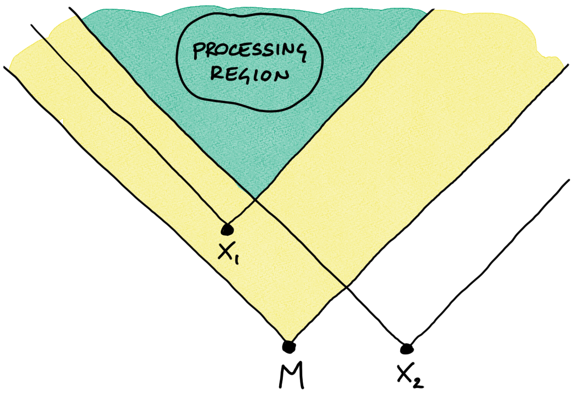
(a) Pair of spacetime points for which PGM propose calculating $w(x_{1},x_{2})$ via P2. The causal future of the measurement $M$ (yellow) contains the overlap of those of $x_{1}$ and $x_{2}$ (green). Consequently, the processing region for $w(x_{1},x_{2})$ is contained in the causal future of the measurement. As it is clear, information collected at both $x_{1}$ and $x_{2}$ is only available to MIOs knowing the measurement outcome, and the usage of P2 is justified.

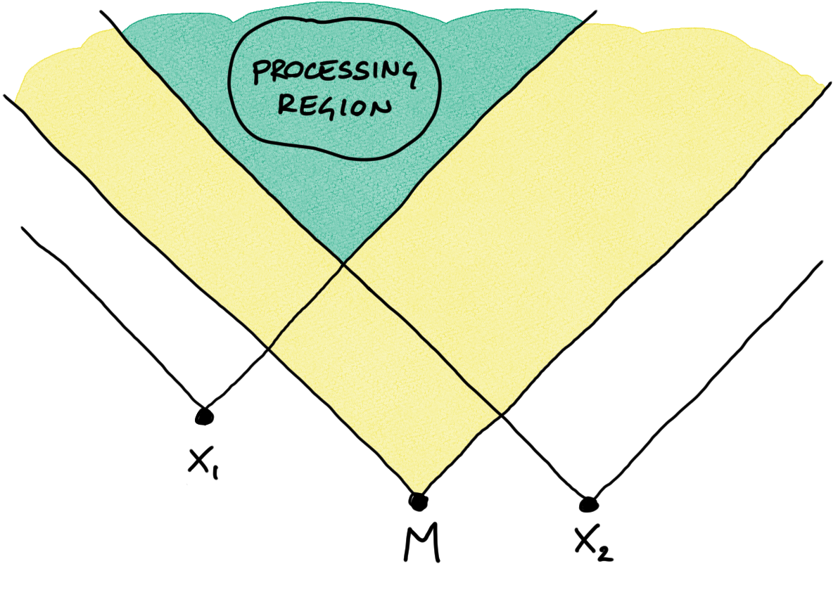
(b) Pair of spacetime points for which calculating $w(x_{1},x_{2})$ via P1-P2 is ill-defined. The causal future of the measurement $M$ (yellow) contains the overlap of the causal futures of $x_{1}$ and $x_{2}$ (green), and hence the processing region for $w(x_{1},x_{2})$. While P1 says to use the state of the MIO outside the yellow region, the logic leading to P2 says we should use the state of the MIO inside the yellow region, leading to a contradiction.

Figure 1: Localization of the processing region for the two-point function $w(x_{1},x_{2})$. On the left is an example of the setting for which P2 was introduced; on the right is one case for which using P1-P2 leads to a contradiction.

I.2 Second issue: two-point functions across and outside a measurement’s future light cone

The second issue arises from using PGM’s contextual states to calculate $n$-point correlation functions. As evident, the proposed contextual nature of QFT states renders the usual rule for calculating $n$-point functions inadequate, as correlation functions not only depend on the field operators at the points they are inserted in, but also on the observers assigning the state to compute the correlation function. To better formalise this idea, PMG introduce the notion of the processing region of a $n$-point function (see also [8]). Given a set of points $\{x_{1},\dots,x_{n}\}$ over which one wants to calculate the $n$-point function $w(x_{1},\dots,x_{n})$, the processing region is a portion of spacetime contained in the intersection of future lightcones of these points, meaning that messages carrying information about the events labelled by $x_{1},\dots,x_{n}$ can reach observers in the processing region. Therefore, computation of correlation functions for operators inserted in $x_{1},\dots,x_{n}$ must be ”performed” by maximally informed observers in the processing region, able to use the appropriate state for the computation.

Let us view the details of how this construction affects the computation of $n$-point functions by considering a spacetime that contains only one measurement $M$. In this case, PGM propose the following prescription to calculate $n$-point functions:

• if the points are all inside (all outside) the measurement’s future light cone, use

  $$w(x_{1},\dots,x_{n})=\textrm{Tr}[\rho\phi(x_{1}),\dots,\phi(x_{n})]~{},$$ (4)

  where $\rho$ is the contextual field’s state relative to the MIO inside (outside) the future light cone of the measurement.

• if the points are both inside and outside $M$’s future light cone, use

  $$w(x_{1},\dots,x_{n})=\textrm{Tr}[\rho^{\prime}\phi(x_{1}),\dots,\phi(x_{n})]~{}.$$ (5)

  where $\rho^{\prime}$ is the contextual field’s state relative to the MIO inside the future light cone of the measurement.

The reason for using the state relative to the MIO inside the future light cone of the measurement in P2 is that, for $n>1$, $n$-point functions are non-local quantities that must locally be computed. To do so, an observer willing to calculate a $n$-point function should wait until the necessary (locally collected) information reaches some processing region which, in P2, is always included in the future light cone of the measurement; hence, the state relative to the MIO of that region must be used in this case (see Fig. 1(a)).

However, the prescription is inconsistent for $n$-point functions evaluated outside the light cone. To show this, let us consider $w(x_{1},x_{2})$ with $x_{1}$ and $x_{2}$ outside the future of the measurement and such that the overlap of their causal futures is fully contained in the future of the measurement, as in Fig. 1(b). As both points lay outside the future of the measurement, PGM’s prescription tells us to use P1, hence calculating $w(x,y)$ by the state of the MIO of the observer laying outside the future of the measurement. However, the processing region for this setting must be contained in the future light cone of the measurement, and any observer computing the two-point function has the knowledge given by the selective update and could use P2 instead. Therefore, P1 and P2 give conflicting prescriptions for this scenario. The issue is solved if one gives states a spacetime dependence and employs algebraic tools, using the state relative to each point appearing in $w(x,y)$ to calculate the two-point function.

In Section V, we employ algebraic tools to expand upon the QFT state assignment introduced in Sec. IV for addressing the first issue, and we discuss their effectiveness in resolving the inconsistencies related to $n$-point functions.

Notation and conventions

Throughout the article, we use the following notation and conventions. We denote spacetime points with lowercase letters (e.g. $x$, $y$, etc.), their spatial part by bold lowercase letters (e.g. $\mathbf{x}$, $\mathbf{y}$, etc.), and sets of spacetime points with uppercase letters (e.g. $A$, $B$, etc.). As it will be discussed in Sec. II.2, measurements are also read as sets of spacetime events, denoted by uppercase letters. The spacetime is Hausdorff, time-orientable and has metric with signature $(-,+,\dots)$. The causal future of a spacetime region $A$, denoted by $\mathcal{J}^{+}(A)$, is the set of all points which can be reached from $A$ by future-directed non-spacelike curves, and the domain of future dependence of $A$, denoted by $\mathcal{D}^{+}(A)$, is the set of all points $x$ such that every past-inextendible non-spacelike curve through $x$ intersects $A$. The causal past $\mathcal{J}^{-}(\cdot)$ and domain of past dependence $\mathcal{D}^{-}(\cdot)$ are defined similarly [9]. From these, we build $\mathcal{J}(A)=\mathcal{J}^{+}(A)\cup\mathcal{J}^{-}(A)$ and $\mathcal{D}(A)=\mathcal{D}^{+}(A)\cup\mathcal{D}^{-}(A)$. Finally, observers will be denoted by calligraphic capital letters (e.g. $\mathcal{A}$ for Alice, $\mathcal{B}$ for Bob, etc.).

II Refined detector-based measurements in QFT

The Unruh-DeWitt model for particle detectors was introduced as a tool for studying the notion of particles in QFT in curved and non-inertial spacetimes [10, 11, 12, 13, 14]. For the purpose of this article, it is sufficient to consider the simple setting of a bipartite system composed of a two-level Unruh-DeWitt detector $M$ with non-degenerate free Hamiltonian

$$\hat{H}_{M}=\omega\ket{1}\bra{1}~{},$$ (6)

and a real massive scalar quantum field $\phi$ with Hamiltonian $\hat{H}_{\phi}$. In addition to the global free Hamiltonian

$$\hat{H}=\hat{H}_{M}+\hat{H}_{\phi}$$ (7)

the detector and the field interact via the (detector’s proper) time-dependent Hamiltonian

$$\hat{H}_{\mathrm{int}}(\tau)=\chi(\tau)\hat{m}(\tau)\otimes\hat{\phi}_{f}(\tau)~{},$$ (8)

where $\chi(\tau)$ is a smooth switching function describing the interaction’s duration and intensity,

$$\hat{m}(\tau)=e^{-i\omega\tau}\ket{1}\bra{0}+e^{i\omega\tau}\ket{0}\bra{1}$$ (9)

is the detector’s monopole momentum operator in the interaction picture, and $\hat{\phi}_{f}(\tau)$ is a spatially smeared field operator describing the detector’s spatial profile [15, 16, 17] along the detector’s world line

$$x(\tau)=(t(\tau),\mathbf{x}(\tau))~{}.$$ (10)

Finally, $\hat{H}_{\mathrm{int}}(\tau)$ is often multiplied by a small constant $\lambda$ to make the interaction weak and allow the usage of perturbation theory. In PMG’s framework, these detectors are used as a probe to test the field; in the rest of this section, we discuss how this is made, refining some details about the model along the way.

II.1 Non-relativistic measurements

In order to frame our later discussion, it is crucial to have a robust description of non-relativistic measurements and their reading as sets of spacetime events. In non-relativistic QM, one can introduce a measurement by the so-called positive operator-valued measure (POVM): a map $O$ from the family of parts $\mathcal{M}$ of the set of possible outcomes of the measurement $R=\{E_{0},E_{1}\dots\}$ to the set of hermitian operators acting on the Hilbert space of the measured system, i.e.

$$O:\mathcal{M}\longrightarrow op(\mathcal{H})~{},$$ (11)

such that

$$\hat{O}(E_{l})\equiv\hat{E}_{l}\geq 0$$ (12)

$$\hat{O}(R)=\mathbb{I}$$ (13)

$$\hat{O}(\cup_{l}E_{l})=\sum_{l}\hat{O}(E_{l})=\sum_{l}\hat{E}_{l}$$ (14)

In particular, since the measurement operators are positive, we can always find a set of operators $\hat{M}_{i}$ such that

$$\hat{E}_{i}=\hat{M}^{\dagger}_{i}\hat{M}_{i}~{},$$ (15)

and hence rewrite Eq. (13) as

$$\sum_{i}\hat{M}^{\dagger}_{i}\hat{M}_{i}=\mathbb{I}~{}.$$ (16)

Although the above framework provides a mathematical description of measurements, it does not encompass all the physical aspects involved in actual measurements performed in labs. Specifically, a quantum measurement involves a collapse phenomenon that extends beyond POVMs alone. Nevertheless, one can define a minimal description of measurements via POVMs as follows. For any element $E_{i}\in R$, the number

$$p^{O}_{\rho}(E_{i})=\textrm{Tr}[\rho\hat{O}(E_{i})]$$ (17)

is the probability that an experimental observation associated with the measurement $O$ of the system in the state $\rho$ gives the result $E_{i}$. If the outcome $E_{i}$ is realized, the state of the system makes the (non-unitary) jump

$$\rho\longmapsto\rho_{i}=\frac{\hat{M}_{i}\rho\hat{M}_{i}^{\dagger}}{\textrm{Tr}[\hat{M}_{i}\rho\hat{M}_{i}^{\dagger}]}~{}.$$ (18)

The update of the system’s state via Eq. (18) is usually called measurement-induced state collapse, or Lüders rule.

II.2 Detector-based measurements as sets of events

PGM’s framework utilises non-relativistic measurements to establish a measurement procedure in the context of QFT. This is achieved through non-relativistic systems, such as Unruh-DeWitt detectors, as mediators to measure quantum fields. Specifically, one lets a non-relativistic system interact with a quantum field and measures the former to extract information about the latter. Here, we refine PMG’s measurements on quantum fields by considering all relevant parts of non-relativistic measurements in the description, including the (unspecified) process that generates the measurement output. Therefore, a detector-based measurement on a quantum field is composed of three processes:

1. the detector and the field are entangled via some unitary interaction. This allows for later extraction of information about the field by measurements performed on the detector via the von Neumann scheme [18, 19]. The spacetime region containing (at least) all events comprising this interaction is called $M_{c}$.

2. the POVM performed on the detector and the related output production, which is the process making the (non-unitary) transition (18) to occur. Different interpretations of QM disagree on the specific microscopic realization of the output production [20]; for the sake of generality, here we only assume there is some kind of unspecified process realizing (18), and it can be represented by a collection of events included in a spacetime region $M_{o}$.

3. a delay, necessary for making a large enough region of spacetime (typically having the size around that of the detector) aware of the obtained result. The delay is defined as a set $M_{d}$ such that every $p\in M_{d}$ satisfying $\mathcal{J}^{+}(p)\cap M_{d}=\{p\}$ is contained in the future of the future endpoint of lightlike curves on the boundary of $\mathcal{D}^{+}(M_{o})$.

Notice that the relation $M_{o}\subset\mathcal{J}^{+}(M_{c})$ must be satisfied. For the sake of simplicity, we assume that the three spacetime subsets are connected, and any measurement $M$ is simply the union $M=M_{c}\cup M_{o}\cup M_{d}$. Furthermore, we call $\mathcal{P}_{M}$ the region in which the classical information about the measurement’s outcome is available, which corresponds to the causal future of all points $p\in M$ satisfying $\mathcal{J}^{+}(p)\cap M=\{p\}$. An example of a measurement’s spacetime structure is represented in Fig. 2.

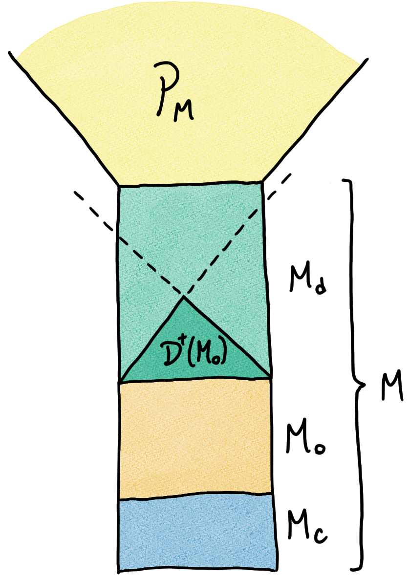
Figure 2: Spacetime structure of a measurement. The measurement is composed of the detector-field coupling $M_{c}$ (blue), the output production (orange) and a delay region $M_{d}$ (green) built in such a way that all points whose future contains no measurement points have access to the measurement output. To obtain this, it is sufficient that these are in the future of the ”latest” point of $\mathcal{D}^{+}(M_{o})$ (dark green), whose future light cone is represented by dotted lines. Finally, the region $\mathcal{P}_{M}$ (yellow) is a collection of events where the measurement output is accessible.

III Two detectors: a case study

Let us now consider the case where two detectors $A$, $B$ interact with the same massive real scalar field $\phi$. Given a spacelike foliation of the spacetime $\Sigma_{t}$ parametrized by $t$, the interaction Hamiltonian of the two detectors with the field is taken to be

$$\hat{H}_{int}(t)=\hat{H}_{A}(\tau_{A})+\hat{H}_{B}(\tau_{B})~{},$$ (19)

where the interaction Hamiltonians are those of Eq. (8) and the relation $\tau_{A,B}(t)$ is provided by $\Sigma_{t}$. In the following, we identify a detector with its measurement region and consider:

• the future light cone $\mathcal{J}^{+}(I)$ of the detector $I$, for $I=A,B$;

• the future light cone of the events corresponding to the measurement output production and read-out $\mathcal{P}_{I}$, for $I=A,B$.

Following Ref. [1], we study the field as seen by a third detector $C$ when the detectors $A$ and $B$ are spacelike to each other, and neither $A$ nor $B$ are in the future of $C$. Therefore, we define the region

$$\mathcal{S}_{AB}=\mathcal{M}/(\mathcal{J}(A)\cup\mathcal{J}(B))~{},$$ (20)

i.e. the region of spacetime that is spacelike to both $A$’s and $B$’s past and future. Three scenarios are then defined by the causal relation between $A$ and $B$ and the third detector. In particular, $C$ can be:

1. spacelike separated from both $A$ and $B$, i.e. $C\subset\mathcal{S}_{AB}$: an observer measuring $C$ after its interaction with the field would have no information about the outcomes of measurements performed on $A$ or $B$.

2. in $\mathcal{P}_{A}/\mathcal{P}_{B}$ (or $\mathcal{P}_{B}/\mathcal{P}_{A}$): an observer can access the measurement outcome of $A$ ($B$) but not that of $B$ ($A$).

3. in $\mathcal{P}_{A}\cap\mathcal{P}_{B}$: an observer measuring $C$ can access both the outcomes obtained by $A$ and $B$.

These three possibilities are summarized in Fig. 3, where the relevant spacetime regions are highlighted by different colours.

Working under the assumption that no interaction happened before the measurements, the composite system made of the detectors and the field can be taken to initially be in the pure state

$$\ket{\psi}=\ket{\phi_{0}}\otimes\ket{\alpha}\otimes\ket{\beta}~{}.$$ (21)

Hence, the initial state of the field in the density operator formalism is

$$\rho_{\phi_{0}}=\ket{\phi_{0}}\bra{\phi_{0}}~{}.$$ (22)

Notice that while this state depends on the specific slicing used to define the time evolution of spacelike sub-manifolds, there is always a way to select a Cauchy slice in the past of the interactions (i.e. that it does not intersect the detector regions) for which the state of the field is a projector. For later convenience, we also define the initial detectors’ density operators

$$\sigma_{\kappa}=\ket{\kappa}\bra{\kappa}$$ (23)

for $\kappa=\alpha,\beta$; therefore, the state in Eq. (21) can also be expressed as

$$\rho_{0}=\rho_{\phi_{0}}\otimes\sigma_{\alpha}\otimes\sigma_{\beta}~{}.$$ (24)

Moreover, since $A$ and $B$ are spacelike separated, the operators in $\hat{H}_{A}(\tau_{A}),\hat{H}_{B}(\tau_{B})$ commute, hence the the time evolution operator $U(t;t_{0})$ in the interaction picture satisfies

$$U(t;t_{0})=U_{A}(t;t_{0})U_{B}(t;t_{0})~{},$$ (25)

with $[U_{A}(t;t_{0}),U_{B}(t;t_{0})]=0$, regardless of the slicing considered. Furthermore, it is worth noting that different slicing choices give different field and detector states at the same spatial location: while surprising, it will be clear from the later discussion that this does not affect physical results, and, in our proposal, all these states are related by an equivalence relation making the slicing choice irrelevant.

Before analysing the above three cases, let us briefly mention that these do not exhaust all possible regions where one can find $C$. For example, the spacetime strips $\mathcal{J}^{+}(I)/\mathcal{P}(I)$, $I=A,B$, are not covered by the above discussion. This is due to the difficulty of modelling contemporary interactions. The case in which $C$ is in these spacetime regions will not be considered for the rest of the article.

We now study how to assign a state for a scalar quantum field $\phi$ in the case of the detector $C$ being measured when in the regions

1. $C\subset\mathcal{S}_{AB}$

2. $C\subset\mathcal{P}_{A}/\mathcal{P}_{B}$ and $C\subset\mathcal{P}_{B}/\mathcal{P}_{A}$

3. $C\subset\mathcal{P}_{A}\cap\mathcal{P}_{B}$

The only region having clear causal relation with $A$ and $B$ left out of our analysis is that identified by the causal pasts of $A$ and $B$, for which the discussion is trivial.

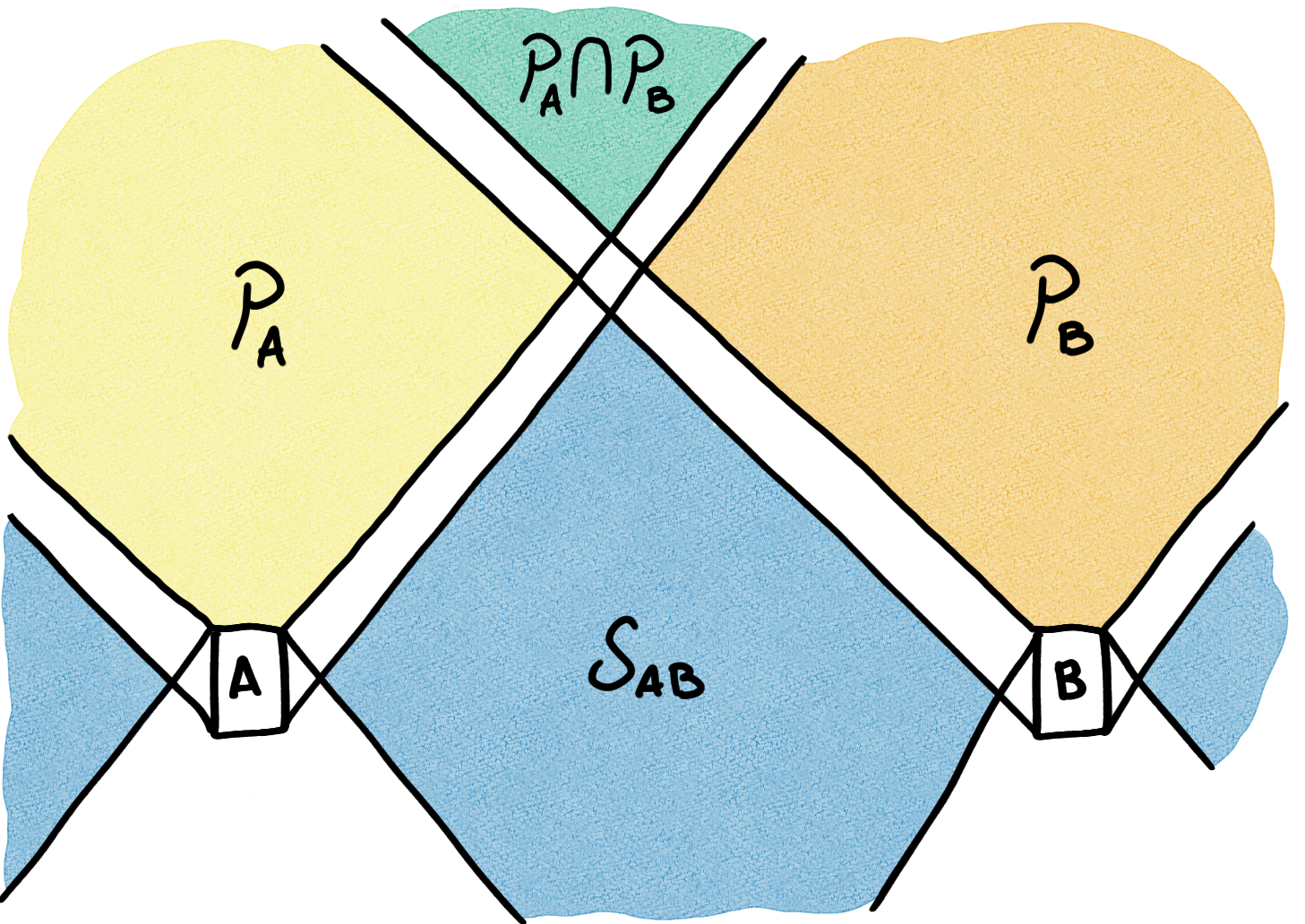
Figure 3: Causal diagram for two space-like separated detectors. The blue region, called $\mathcal{S}_{AB}$, is the region space-like separated from the detectors $A$ and $B$. The yellow (orange) region, called $\mathcal{P}_{A}$ ($\mathcal{P}_{B}$), is the future light cone of a set of points containing the events where the output of a measurement performed on $A$ ($B$) is known. The green region, called $\mathcal{P}_{A}\cap\mathcal{P}_{B}$, is the set of points that are in the future light-cone of the output production of both $A$ and $B$.

III.1 $C\subset\mathcal{S}_{AB}$

First, we consider the case when $C$ is spacelike to $A$ and $B$, i.e. $C\subset\mathcal{S}_{AB}$. In this case, the possible states of knowledge of $\mathcal{O}_{C}$ about the measurements performed on $A$ and $B$ are:

1. $\mathcal{O}_{C}$ does not know $\mathcal{O}_{A}$ and $\mathcal{O}_{B}$ performed measurements
   $\Rightarrow$ its field’s state is $\rho_{\bf 1}\equiv\rho_{\mathcal{S}_{AB}}=\rho_{\phi_{0}}$;

2. $\mathcal{O}_{C}$ only knows $\mathcal{O}_{A}$ performed a measurement (but not the outcome)
   $\Rightarrow$ its field’s state is $\rho_{\bf 2}\equiv\rho^{A}_{\mathcal{S}_{AB}}$;

3. $\mathcal{O}_{C}$ only knows $\mathcal{O}_{B}$ performed a measurement (but not the outcome)
   $\Rightarrow$ its field’s state is $\rho_{\bf 3}\equiv\rho^{B}_{\mathcal{S}_{AB}}$;

4. $\mathcal{O}_{C}$ knows that both $\mathcal{O}_{A}$ and $\mathcal{O}_{B}$ performed measurements (but not the outcomes)
   $\Rightarrow$ its field’s state is $\rho_{\bf 4}\equiv\rho^{AB}_{\mathcal{S}_{AB}}$;

The states related to the above points 2 and 3 are obtained by the partial trace over $\mathcal{H}_{A}$ and $\mathcal{H}_{B}$ of the state of as it is described by $\mathcal{O}_{C}$. For example, in the case 2 the state before the trace is

$$\left(\sum_{a}\mathbb{I}\otimes\hat{M}_{a}(\hat{U}_{A}\rho_{\phi_{0}}\otimes\rho_{\alpha}\hat{U}_{A}^{\dagger})\mathbb{I}\otimes\hat{M}^{\dagger}_{a}\right)\otimes\rho_{\beta}\otimes\rho_{\gamma}$$ (26)

which, after the partial trace, gives

$$\rho_{\bf 2}=\rho^{A}_{\mathcal{S}_{AB}}=\textrm{Tr}_{A}[\hat{U}_{A}(\rho_{\phi_{0}}\otimes\rho_{\alpha})\hat{U}_{A}^{\dagger}]~{};$$ (27)

similarly, in case 3 one gets

$$\rho_{\bf 3}=\rho^{B}_{\mathcal{S}_{AB}}=\textrm{Tr}_{B}[\hat{U}_{B}(\rho_{\phi_{0}}\otimes\rho_{\beta})\hat{U}_{B}^{\dagger}]~{}.$$ (28)

Finally, the density operator $\rho_{\bf 4}$ is obtained by the same procedure, where now the states of both $A$ and $B$ are those obtained by a non-selective update rule, hence giving

$$\rho_{\bf 4}=\textrm{Tr}_{AB}[\hat{U}_{A}\hat{U}_{B}(\rho_{\phi_{0}}\otimes\rho_{\alpha}\otimes\sigma_{\beta})\hat{U}_{A}^{\dagger}\hat{U}^{\dagger}_{B}]~{}.$$ (29)

For the picture to be consistent, it must be that all locally supported field observables $\mathcal{O}_{C}$ one can measure have the same expectation value when evaluated via the density operators 1-4, i.e.

$$\textrm{Tr}[\rho_{\bf 1}\hat{L}]=\textrm{Tr}[\rho_{\bf 2}\hat{L}]=\textrm{Tr}[\rho_{\bf 3}\hat{L}]=\textrm{Tr}[\rho_{\bf 4}\hat{L}]$$ (30)

when $\hat{L}$ is an observable supported in $\mathcal{S}_{AB}$. Specifically, we call $\mathfrak{O}(R)$ the set of all observables whose support is causally convex and contained in the region $R$. The validity of the above chain of equalities was obtained in Ref. [1] by using the cyclic property of the trace and the fact that, since $A$, $B$ and $\mathcal{S}_{AB}$ are space-like separated, $[\hat{U}_{A},\hat{U}_{B}]=0$ and

$$[\hat{L},\hat{U}_{A}]=[\hat{L},\hat{U}_{B}]=0~{}.$$ (31)

Hence, an observer that is spacelike to both $A$ and $B$ can use any density operator among 1-4 and get the right expectation values. More generally, any density operator in the equivalence class

$$\varrho_{\mathcal{S}_{AB}}=\{\rho~{}|~{}\textrm{Tr}[\rho\hat{L}]=\textrm{Tr}[\rho_{\phi_{0}}\hat{L}],~{}\forall\hat{L}\in\mathfrak{O}(\mathcal{S}_{A,B})\}$$ (32)

gives the correct physical results and can be used as the field’s density operator.

III.2 $C\subset\mathcal{P}_{A}/\mathcal{P}_{B}$ and $C\subset\mathcal{P}_{B}/\mathcal{P}_{A}$

Next, let us consider the case in which the detector $C$ is space-like to $B$ and in the causal future of $\mathcal{P}_{A}$, i.e. when $C\subset\mathcal{P}_{A}/\mathcal{P}_{B}$. In addition to the possible contextual field’s states of knowledge 1-4 above, an observer in this region can also describe the field state in accordance with the following:

1. $\mathcal{O}_{C}$ only knows $\mathcal{O}_{A}$ performed a measurement and the outcome $a$
   $\Rightarrow$ it’s field state is $\rho_{\bf 5}=\rho^{A(a)}_{\mathcal{P}_{A}}$;

2. $\mathcal{O}_{C}$ knows $\mathcal{O}_{A}$ performed a measurement and the outcome $a$, and knows $\mathcal{O}_{B}$ performed a measurement but not the outcome
   $\Rightarrow$ it’s field state is $\rho_{\bf 6}=\rho^{A(a)B}_{\mathcal{P}_{A}}$;

The above states are obtained by the Lüders rule as

$$\rho^{A(a)}_{\mathcal{P}_{A}}=\frac{\textrm{Tr}_{A}[\hat{M}_{a}\hat{U}_{A}(\rho_{\phi_{0}}\otimes\sigma_{\alpha})\hat{U}^{\dagger}_{A}\hat{M}^{\dagger}_{a}]}{\textrm{Tr}[\hat{M}_{a}\hat{U}_{A}(\rho_{\phi_{0}}\otimes\sigma_{\alpha})\hat{U}^{\dagger}_{A}\hat{M}^{\dagger}_{a}]}$$ (33)

and

$$\rho^{A(a)B}_{\mathcal{P}_{A}}=\frac{\textrm{Tr}_{AB}[\hat{M}_{a}\hat{U}_{B}\hat{U}_{A}(\rho_{\phi_{0}}\otimes\sigma_{\alpha}\otimes\sigma_{\beta})\hat{U}^{\dagger}_{A}\hat{U}^{\dagger}_{B}\hat{M}^{\dagger}_{a}]}{\textrm{Tr}[\hat{M}_{a}\hat{U}_{B}\hat{U}_{A}(\rho_{\phi_{0}}\otimes\sigma_{\alpha}\otimes\sigma_{\beta})\hat{U}^{\dagger}_{A}\hat{U}^{\dagger}_{B}\hat{M}^{\dagger}_{a}]}$$ (34)

where we used the cyclic property of the trace and Eq. (16).

Clearly enough, one could consider the case where $C$ lies in $\mathcal{P}_{B}/\mathcal{P}_{A}$, and get similar results. In this case, the possible contextual field’s state is one of the 1-4 above or one of the following:

1. $\mathcal{O}_{C}$ only knows $\mathcal{O}_{B}$ performed a measurement and the outcome $b$
   $\Rightarrow$ it’s field state is $\rho_{\bf 7}=\rho^{B(b)}_{\mathcal{P}_{B}}$;

2. $\mathcal{O}_{C}$ knows $\mathcal{O}_{B}$ performed a measurement and the outcome $b$, and knows $\mathcal{O}_{A}$ performed a measurement but not the outcome
   $\Rightarrow$ it’s field state is $\rho_{\bf 8}=\rho^{AB(b)}_{\mathcal{P}_{B}}$;

Similarly to the above, one obtains the states 7 and 8 in the same way as (33-34) but with different upper and lower indices. The compatibility between 5 and 6 (7 and 8) was proven in Ref. [1] by the same tools used for proving the equivalence of 1-4.

However, 5-6 are not compatible with 1-4 (while this could be proven also for 7-8, here we limit our analysis to the former for the sake of simplicity). To prove this statement, we consider some field operator $\hat{L}\in\mathfrak{O}(\mathcal{P}_{A}/\mathcal{P}_{B})$ and confront its expectation value as observed by the observer $\mathcal{O}_{A}$ (having maximal information available, hence using the density operator $\rho_{\bf 6}$ or, equivalently, $\rho_{\bf 5}$) and $\mathcal{O}_{C}$, using any density operator in the equivalence class (32). As claimed above, when using $\rho\in\varrho_{\mathcal{S}_{AB}}$ the expectation value of an operator $\hat{L}$ is

$$\langle\hat{L}\rangle_{\rho}=\textrm{Tr}[\rho_{\phi_{0}}\hat{L}]~{},$$ (35)

which can be expressed equivalently by means of $\rho_{\bf 2}$ as

$$\langle\hat{L}\rangle_{\bf 2}=\textrm{Tr}[\hat{U}_{A}(\rho_{\phi_{0}}\otimes\sigma_{\alpha})\hat{U}^{\dagger}_{A}\hat{L}]~{}.$$ (36)

On the contrary, using $\rho_{\bf 5}$ gives

$$\langle\hat{L}\rangle_{\bf 5}=\frac{\textrm{Tr}[\hat{M}_{a}\hat{U}_{A}(\rho_{\phi_{0}}\otimes\sigma_{\alpha})\hat{U}^{\dagger}_{A}\hat{M}^{\dagger}_{a}\hat{L}]}{\textrm{Tr}[\hat{M}_{a}\hat{U}_{A}(\rho_{\phi_{0}}\otimes\sigma_{\alpha})\hat{U}^{\dagger}_{A}\hat{M}^{\dagger}_{a}]}~{}.$$ (37)

By calling $\rho^{\prime}=\hat{U}_{A}\rho_{\phi_{0}}\otimes\sigma_{\alpha}\hat{U}^{\dagger}_{A}$ and $\hat{M}_{a}\hat{M}_{a}^{\dagger}=\hat{\Gamma}$, we get that

$$\langle\hat{L}\rangle_{\bf 2}=\langle\hat{L}\rangle_{\bf 5}~{}\Leftrightarrow~{}\textrm{Tr}[\rho^{\prime}\hat{L}\hat{\Gamma}]=\textrm{Tr}[\rho^{\prime}\hat{L}]\times\textrm{Tr}[\rho^{\prime}\hat{\Gamma}]~{},$$ (38)

for all $\hat{L}$, which is only satisfied when $\hat{\Gamma}=\mathbb{I}$ (see App. A), and hence

$$\langle\hat{L}\rangle_{\bf 2}=\langle\hat{L}\rangle_{\bf 5}~{}\Leftrightarrow~{}\hat{M}^{\dagger}_{a}\hat{M}_{a}\propto\mathbb{I}~{}.$$ (39)

However, in order to describe a non-trivial measure, the measurement operator must satisfy $\hat{M}^{\dagger}_{a}\hat{M}_{a}\neq k\mathbb{I}$, where $k$ is some proportionality constant. Hence, the density operators of 5-6 (and 7-8) are not equivalent to those of Eq. (32). More generally, by defining the equivalence classes

$$\varrho_{\mathcal{P}_{A}/\mathcal{P}_{B}}=\{\rho~{}|~{}\textrm{Tr}[\rho\hat{L}]=\textrm{Tr}[\rho_{\bf 6}\hat{L}],~{}\forall\hat{L}\in\mathfrak{O}(\mathcal{P}_{A}/\mathcal{P}_{B})\}$$ (40)

and

$$\varrho_{\mathcal{P}_{B}/\mathcal{P}_{A}}=\{\rho~{}|~{}\textrm{Tr}[\rho\hat{L}]=\textrm{Tr}[\rho_{\bf 8}\hat{L}],~{}\forall\hat{L}\in\mathfrak{O}(\mathcal{P}_{B}/\mathcal{P}_{A})\}$$ (41)

we get that the expectation values of operators having support in $\mathcal{P}_{A}/\mathcal{P}_{B}$ and $\mathcal{P}_{A}/\mathcal{P}_{B}$ evaluated by means of a representative of (40) and (41) respectively are different from those obtained by using a representative of $\sigma_{\mathcal{S}_{AB}}$. Therefore, observers that enter $\mathcal{P}_{A}/\mathcal{P}_{B}$ or $\mathcal{P}_{B}/\mathcal{P}_{A}$ cannot use the density operators of (32) and get the right statistics.

III.3 $C\subset\mathcal{P}_{A}\cap\mathcal{P}_{B}$

Finally, we consider the case in which the detector $C$ is in the causal future of both $\mathcal{P}_{A}$ and $\mathcal{P}_{B}$, i.e. $C\subset\mathcal{P}_{A}\cap\mathcal{P}_{B}$. In this case, the contextual state of knowledge about the field can be one of the above 1-8 or

1. $\mathcal{O}_{C}$ knows the outcomes of the measurements performed by $\mathcal{O}_{A}$ and $\mathcal{O}_{B}$, which are $a$ and $b$ respectively
   $\Rightarrow$ it’s field state is $\rho_{\bf 9}=\rho^{A(a)B(b)}_{\mathcal{P}_{A}\cup\mathcal{P}_{B}}$;

However, no density operator in the equivalence classes $\sigma_{\mathcal{S}_{AB}}$, $\sigma_{\mathcal{P}_{A}/\mathcal{P}_{B}}$ or $\sigma_{\mathcal{P}_{B}/\mathcal{P}_{A}}$ is able to give the same expectation values as those obtained by $\rho_{\bf 9}$, i.e.

$$\langle\hat{L}\rangle_{\bf 9}\neq\langle\hat{L}\rangle_{\bf j}~{},\forall{\bf j}=1,\dots,8$$ (42)

The proof of this fact is similar to that of the above paragraph, and it can be found in App. B. As a consequence, we define a new equivalence class

$$\varrho_{\mathcal{P}_{B}\cap\mathcal{P}_{A}}=\{\rho~{}|~{}\textrm{Tr}[\rho\hat{L}]=\textrm{Tr}[\rho_{\bf 9}\hat{L}],~{}\forall\hat{L}\in\mathfrak{O}(\mathcal{P}_{B}\cap\mathcal{P}_{A})\}$$ (43)

describing all the states that one can assign to the field while being in $\mathcal{P}_{B}\cap\mathcal{P}_{A}$.

IV Equivalence classes of density operators

The result of the above discussion is that density operators are not contextual to observers using them: indeed, we can imagine observers that do not know the outcomes of the measurements performed in their past light cone and get the wrong results when trying to use non-updated density operators. On the contrary, we showed that it is possible to assign an equivalence class of density operators to each spacetime region belonging to the causal future of measurements or to those regions spacelike to the interaction between detectors and the field; these density operators can be seen as those contextual to the maximally informed observer of Sec. I.1.

IV.1 Solving the first issue

Assuming there always is an initial pure state for the field $\rho_{0}$ (in our case, the vacuum), each equivalence class contains a state obtained by the initial one via a quantum map $\mathcal{E}^{(\textbf{a})}$ depending on all measurements’ outcomes a performed in the causal past of the region related to the class. Therefore we can always write

$$\varrho_{R}=\{\rho~{}|~{}\textrm{Tr}[\rho\hat{L}]=\textrm{Tr}[\mathcal{E}^{(\textbf{a})}(\rho_{0})\hat{L}]~{},~{}\forall\hat{L}\in\mathfrak{A}(R)\}$$ (44)

where the all measurements giving the outcomes a belong to $\mathcal{J}^{-}(R)$, and $\mathfrak{A}(R)$ is the set of all observables localised in the (causally convex) region $R$ considered.

Assigning an equivalence class of density operators instead of a single representative to a system is not new; the procedure is similar to assigning to systems vectors up to a phase. The novelty of our proposal is in how the equivalence classes are constructed and the fact that they depend on the spacetime region in which the system is described, in a way similar to that proposed by Hellwig and Krauss in Ref. [5]. When this idea is pushed forward, it is natural to ask:

1. is it possible to assign an equivalence class of field states to any causally convex spacetime region $R$?

2. if yes, is there a globally-defined state such that, for any $R$, a restriction operation can be applied on it to obtain the field’s state in that region?

In the following, we will show that the answer to these questions is positive when considering spacetime regions $R$ having a definite causal relationship with all measurements in spacetime, and abandoning the idea of density operators being the most general state assignment for quantum systems. To do so, we must consider a more general version of QFT, called algebraic quantum field theory (AQFT). It is interesting to note that the connection between detector-based measurements and AQFT was already hinted at by PGM in Ref. [1], and that algebraic states are part of the FV proposal for measurements in QFT [6, 22].

Before proceeding, we stress that we did not address how to assign equivalence classes to the regions lightlike to measurements and how the transition from a pre-measurement to a post-measurement equivalence class is realised – these questions are beyond the scope of this article.

V Equivalence classes of algebraic states

In the above section, we assigned an equivalence class of density operators to each region $R$ having a definite causal relation to all measurements, depending on the outcomes of the measurements performed in $\mathcal{J}^{-}(R)$. While this construction adequately solves the first issue, it remains silent on the evaluation of $n$-point functions, thus leaving the second issue unaddressed (see Sec. I.2 and later discussion). Specifically, in the above discussion we always considered observables belonging to the sets $\mathfrak{O}(R)$ of all observables whose support is causally convex and contained in the region $R$; clearly enough, products of field evaluated on $n$ separate points not always fall in this category. In this section, we claim algebraic states offer a solution to the second issue. Before going into the details of how this is possible, we briefly recall some aspects of our previous discussion about $n$-point functions and better explain why equivalence classes of density operators are insufficient to settle the matter.

The issue is related to the usage of the processing region to assign $n$-point functions: while allowing a more operational notion of the computation of correlation functions, it leads to inconsistent prescriptions for all (but not only, see footnote 4) those $n$-point functions with $n>1$ evaluating over points outside a measurement outcome and having processing region inside the measurement’s future lightcone. The ill-definiteness comes from the fact that, in this case, PMG’s prescription treats the field as real via P1, yet the only observers able to compute $n$-point functions would use their contextual state, as in P2. As it is clear, once the notion of contextual states is removed by our equivalence classes of density operators, the usage of P2 is meaningless. However, using P1 also gives wrong results, as our equivalence classes are not valid over non-causally convex regions (as any region spacelike to the measurement that includes the above $n$ points is). Therefore, our equivalence classes of density operators leave us without suitable tools for computing generic $n$-point functions. Moreover, one should refrain from using these states outside their validity region: while the computation is sometimes formally possible (as they assign a field state across all spacetime) is also essentially wrong: as we will see, algebraic states naturally solve this issue and provide a consistent rule for computing $n$-point functions.

This section aims to convert equivalence classes of density operators to an algebraic setting, allowing us to read the above description in more general terms and solve the issue about $n$-point functions introduced in Sec. I.2.

V.1 The GNS construction

The primitive elements of AQFT are the spacetime $\mathcal{M}$ and a unital $\ast$-algebra $\mathfrak{A}(\mathcal{M})$ defined on it, called the algebra of observables. To each causally convex bounded region $\mathcal{O}\subset M$ we associate a subalgebra $\mathfrak{A}(\mathcal{O})$ of $\mathfrak{A}(\mathcal{M})$, called the algebra of local observables (see Ref. [24] for a pedagogical review, and Ref. [21] for further details). In particular, we require that

$$\mathfrak{A}(O_{1})\subset\mathfrak{A}(O_{2})$$ (45)

for all $O_{1}\subset O_{2}$ (isotony), and

$$[\mathfrak{A}(O_{1}),\mathfrak{A}(O_{2})]=0$$ (46)

whenever $O_{1}$ and $O_{2}$ are spacelike separated (Einstein causality). In general, the elements of $\mathfrak{A}(O)$ have compact support in spacetime [25].

In this setting, a state $\omega$ is an element of the space $\mathfrak{N}(\mathcal{M})=\mathfrak{A}^{*}_{+\mathbb{I}}(\mathcal{M})$ of all normalised positive linear forms on $\mathfrak{A}(\mathcal{M})$, and $\omega(A)$ is the expectation value of $A\in\mathfrak{A}(\mathcal{M})$ over $\omega$. As it is clear, this notion of a state is very different from the one used in QM and QFT, yet it provides all of the operationally accessible elements we expect from states of a physical theory (namely, expectation values and, more generally, probability distributions related to measurement outcomes and all their momenta). The usual vector states are recovered from the algebraic ones via the so-called GNS construction. This is a way to associate a state $\omega$ to a triple $(\pi_{\omega},\mathcal{H}_{\omega},\psi_{\omega})$, composed by a representation $\pi_{\omega}$ of $\mathfrak{A}(\mathcal{M})$ on the Hilbert space $\mathcal{H}_{\omega}$ and a vector $\ket{\psi_{\omega}}\in\mathcal{H}_{\omega}$, such that

$$\omega(A)=\bra{\psi_{\omega}}\pi_{\omega}(A)\ket{\psi_{\omega}}~{}.$$ (47)

Starting from this, one can evaluate the expectation values of observables over other vector states by

$$\omega_{\psi^{\prime}}(A)=\omega(B^{*}AB)=\bra{\psi^{\prime}}\pi_{\omega}(A)\ket{\psi^{\prime}}$$ (48)

where $\ket{\psi^{\prime}}=\pi_{\omega}(B)\ket{\psi_{\omega}}$ is a vector of the representation $\pi_{\omega}$. In particular, we may assume that $\pi_{\omega}$ is cyclic with $\ket{\psi_{\omega}}$ as the cyclic vector, meaning that any vector state of $\mathcal{H}_{\omega}$ can be approximated by $\pi_{\omega}(B)\ket{\psi_{\omega}}$, for some $B\in\mathfrak{A}(\mathcal{M})$. Moreover, for any given GNS representation of some state $\omega$, one can consider the states $\omega_{\rho}$ defined by

$$\omega_{\rho}(A)=\textrm{Tr}[\rho\pi_{\omega}(A)]~{},$$ (49)

where $\rho$ is a positive trace class operator in the space $\mathcal{B}(\mathcal{H}_{\omega})$ of bounded linear operators over $\mathcal{H}_{\omega}$. The set of all states that can be represented in this way is called the folium of $\omega$, and the states contained in it are called normal states. Taking a state (either a density operator or a vector state) of the folium of $\omega$ and making the GNS construction on it will change the Hilbert space, the representation of the selected state and of the algebra’s elements, but not the resulting expectation values.

V.2 Equivalence classes via AQFT

We are now ready to characterise our equivalence classes in terms of algebraic states. To do so, we start from the GNS construction of the vacuum state $\omega_{0}$, i.e. $(\pi_{0},\mathcal{H}_{0},\ket{0})$, and notice that all operators in the above sections can be expressed as

$$\hat{O}=\pi_{0}(O)$$ (50)

for some local observable $O\in\mathfrak{A}(\mathcal{M})$. This is because, by working on the Hilbert space where the vacuum is represented by $\ket{0}$, we were implicitly assuming the GNS construction related to $\omega_{0}$. Then, the density operators $\rho$ identifying the classes $\varrho_{R}$ represent states in the folium of $\omega_{0}$, and the equivalence classes (44) are included in the equivalence classes

$$\Omega_{R}=\{\omega\in\mathfrak{N}(R)~{}|~{}\omega(L)=\textrm{Tr}[\mathcal{E}^{\textbf{a}}(\rho_{0})\pi_{0}(L)]\}$$ (51)

of (algebraic) states over $\mathfrak{A}(R)$, where $R$ is one of the regions identified by the measurements (e.g. $R=\mathcal{S}(M_{1},\dots,M_{n})$). Next, we build a state $\tilde{\omega}$ over $\mathfrak{A}(\mathcal{M})$ whose restriction to $R$ gives (one of) the states in $\Omega_{R}$, i.e.

$$\tilde{\omega}|_{R}=\omega\in\Omega_{R}~{}.$$ (52)

Before proceeding, it is essential to make two important observations. First, notice that the same local state in a given equivalence class can be extended to many inequivalent global states, meaning that it is only a tool for relating local properties of the various regions defined by the measurement. Second, the global state obtained by the above procedure is generally not well-behaved on the boundary of the regions identified by the measurements; in particular, it was proven in Ref. [26] (corollary 3.3 therein) that a normal state in a double cone $\mathcal{D}$ becomes non-normal when restricted to a double cone $\mathcal{D}^{\prime}\subset\mathcal{D}$, and normal states locally defined on $\mathcal{D}^{\prime}$ extend to states on $\mathcal{D}$ that diverge on the boundary of $\mathcal{D}^{\prime}$. While the regions in our construction are not double cones, we still expect a diverging behaviour to appear on the measurement light cone, justified by the discontinuous transition induced by the Lüders rule.

Next, we ask whether we can find a field state over $\mathcal{M}$ that correctly accounts for the expectation value of the product of two local observables $L_{1}$ and $L_{2}$ supported on strictly spacelike double cones contained in two different measurement-defined regions $R_{1}$ and $R_{2}$. To this end, we call $O_{1}\in R_{1}$ and $O_{2}\in R_{2}$ the two double cones enclosing the observables and, by constructing the equivalence classes $\Omega_{R_{1}}$ and $\Omega_{R_{2}}$, restricting a representative of each class to some local state $\omega_{O_{1}}$ and $\omega_{O_{2}}$, and building their extensions $\tilde{\omega}_{1}$ and $\tilde{\omega}_{2}$ over $\mathcal{A}(\mathcal{M})$, it is clear that, in general,

$$\tilde{\omega}_{1}\neq\tilde{\omega}_{2}~{},$$ (53)

and

$$\tilde{\omega}_{1}|_{O_{2}}\neq\tilde{\omega}_{2}|_{O_{2}}=\omega_{O_{2}}$$ (54)

(and vice versa). However, it was demonstrated in Ref. [27] that, for any pair of states defined on strictly spacelike separated regions $O_{1}$ and $O_{2}$ whose algebras satisfy the Schlieder property, there exists a state $\tilde{\omega}_{12}$ which is an extension of the two, and a product state for the von Neumann subalgebras $\mathfrak{M}_{\omega}(O_{1})$ and $\mathfrak{M}_{\omega}(O_{2})$, with $\mathfrak{M}_{\omega}(R)=\pi_{\omega}(\mathfrak{A}(R))^{\prime\prime}$ being the double commutant of the Hilbert space representation of the local algebra. In other words, it is possible to find an extension $\tilde{\omega}_{12}$ such that

$$\tilde{\omega}_{12}(L_{1}L_{2})=\tilde{\omega}_{1}|_{O_{1}}(L_{1})\tilde{\omega}_{2}|_{O_{2}}(L_{2})~{},$$ (55)

for all $L_{i}\in\mathfrak{M}_{\omega}(O_{i})$, $i=1,2$. This property is sometimes called C^∗-independence [29]. Moreover, since the state $\tilde{\omega}_{12}$ is one of the states realizing the extensions of $\omega_{O_{1}}$ and $\omega_{O_{2}}$, we can choose $\tilde{\omega}_{1}=\tilde{\omega}_{2}=\tilde{\omega}_{12}$. As a result, the state $\tilde{\omega}_{12}$ can be used to evaluate expectation values of the product of operators localised in strictly spacelike regions, including $2$-point functions.

By construction, our discussion only holds for strictly spacelike-separated local operators. However, in App. C, we show that any two compact spacelike regions $A$ and $B$ are strictly spacelike. Since local observables have compact support by definition, the above discussion applies to all spacelike local observables. We will discuss the case of timelike separated operators in Sec. V.3.3.

V.2.1 Measurements

For clarity, we here consider two explicit examples using the above construction.

First, let us use the algebraic framework to show that any naive extension of the states of $\Omega_{\mathcal{P}_{M}}$ to $\mathcal{S}_{M}=\mathcal{M}/\mathcal{J}(M)$ gives the wrong global state. To demonstrate this, we consider the case 5 of Sec. III.2, where a detector $M=A$ measures the outcome $a$, known in the causal future region $\mathcal{P}_{M}$, where the appropriate equivalence class corresponds to the state $\rho_{\bf 5}$ given by (33). In turn, in the (strictly) spacelike separated regions of $\mathcal{S}_{M}$, the appropriate state is a restriction of the vacuum $\rho_{0}=\ket{0}\bra{0}$. Hence, this first example illustrates that one cannot naively extend these states to opposite regions, e.g. $\rho_{\bf 5}$ to $\mathcal{S}_{M}$. We start by noticing that the corresponding algebraic states $\omega_{0}$ and $\omega_{\rho_{\bf 5}}$ are both normal states of the representation $\pi_{0}$, i.e.

$$\omega_{0}(L)=\bra{0}\hat{L}\ket{0}$$ (56)

with $\hat{L}=\pi_{0}(L)$, and $L\in\mathfrak{A}(\mathcal{S}_{M})$, and

$$\omega_{\rho_{\bf 5}}(L)=\bra{0}\hat{Q}^{\dagger}\hat{L}\hat{Q}\ket{0}$$ (57)

with $L\in\mathfrak{A}(\mathcal{P}_{M})$, where the operator

$$\hat{Q}=\frac{1}{\sqrt{\textrm{Tr}[\hat{M}_{a}\hat{U}_{A}(\rho_{\phi_{0}}\otimes\sigma_{\alpha})\hat{U}^{\dagger}_{A}\hat{M}^{\dagger}_{a}]}}\bra{\alpha}\hat{U}^{\dagger}_{A}\ket{a}$$ (58)

can be obtained as the $\pi_{0}$-representation of an element $Q$ of the algebra $\mathfrak{A}(M)\subset\mathfrak{A}(\mathcal{M})$. Extending Eq. (57) to hold for elements in $\mathfrak{A}(\mathcal{S}_{M})$, we can use Einstein’s causality and the fact that $\pi_{0}$ is a group homomorphism to get that

$$\omega_{0}(L)=\omega_{\rho_{\bf 5}}(L)$$ (59)

for $L\in\mathfrak{A}(\mathcal{S}_{M})$ holds if and only if

$$\pi_{0}(Q^{*}Q)=\mathbb{I}_{\mathcal{H}_{0}}~{},$$ (60)

which means

$$Q^{*}Q=\mathbb{I}_{\mathfrak{A}(M)}~{}.$$ (61)

However, Eq. (61) does not hold for the $Q$ implicitly defined in Eq. (58) and, more generally, for any $Q\in\mathfrak{A}(\mathcal{M})$ associated with an informative measurement [30, 31]. Hence the incorrect attempt to use $\omega_{\rho_{\bf 5}}(L)$ in $\mathcal{S}_{M}$ (and $\omega_{0}(L)$ in $\mathcal{P}_{M}$) gives wrong expectation values.

The next example illustrates the importance of knowing the outcome $a$ in the region $\mathcal{P}_{M}$. Let us first represent the measurement on $\rho_{0}$ as a quantum channel localized in $M$,

$$\rho=\mathcal{E}(\rho_{0})=\sum_{i}\hat{K}^{\dagger}_{i}\rho_{0}\hat{K}_{i}~{},$$ (62)

where $\{\hat{K}_{i}\}$ are the operators built by the Kraus representation theorem for absolutely local operations [32]. If the outcome of the measurement is known, the above sum reduces to one term corresponding to the obtained outcome (and a normalization is required); otherwise, the measurement is non-selective. As we will see, using $\omega_{0}$ or $\omega_{\rho}$ is equivalent whenever the Kraus operators represent a non-selective measurement. In fact,

$$\omega_{\rho}(L)=\textrm{Tr}[\rho\hat{L}]=\sum_{i}\omega_{0}(K^{*}_{i}LK_{i})~{},$$ (63)

where $\hat{K}_{i}=\pi_{0}(K_{i})$ and, if $L\notin\mathfrak{A}(\mathcal{P}(M))$, then

$$\omega_{\rho}(L)=\omega_{0}\left(L\left[\sum_{i}K^{*}_{i}K_{i}\right]\right)~{},$$ (64)

meaning that $\omega_{0}$ and $\omega_{\rho}$ are in the same equivalence class iff

$$\sum_{i}K_{i}^{*}K_{i}=\mathbb{I}_{\mathfrak{A}(M)}~{}.$$ (65)

Therefore, the equivalence classes of states obtained starting from $\omega_{0}$ and $\omega_{\rho}$ are the same iff the algebra elements associated with the Kraus operators sum up to $\mathbb{I}_{\mathfrak{A}(M)}=\mathbb{I}_{\mathfrak{A}(\mathcal{M})}$, which is the case when the map $\mathcal{E}$ represents a non-selective measurement. Thus the equivalence class of states $\omega_{\rho_{\bf 5}}$, corresponding to a known measurement outcome in $\mathcal{P}_{M}$, must be different. Notice that these results are the algebraic version of the ones obtained in Sec. III, where we proved that different (contextual) density operators do not always give the same expectation values.

V.3 Solving the second issue

We now show how our algebraic state assignment consistently describes one- and two-point functions, solving the issue presented in Sec. I.2. In particular, for a given measurement $M$ we focus our discussion about two-point functions on field operators evaluated at any two points in $\mathcal{P}_{M}$ and $\mathcal{S}_{M}=\mathcal{M}/\mathcal{J}(M)$. However, the construction can be generalised to more measurements and higher order $n$-point functions evaluated in any collection of points belonging to strictly spacelike double cones contained in regions having definite causal relation with all measurements (i.e. in regions that are either spacelike to the measurements or in the future of their output production).

For the rest of this section, we will consider point-wise $n$-point functions, i.e. Wightman functions evaluated on spacetime points. However, these must be read via the nuclear theorem [25] as a tool for calculating the smeared Wightman functions

$$W(f_{1},\dots,f_{n})=\int\prod_{j=1}^{n}dx_{j}f_{j}(x_{j})\langle\phi(x_{1})\dots\phi(x_{n})\rangle~{},$$ (66)

where $f_{i}$ are Schwartz test functions localised in compact regions with definite causal relation with all measurements.

V.3.1 $n$-point functions within measurement regions

First, the rule proposed in Ref. [1] for one-point functions can be applied in our framework without modification, and it reads

$$\braket{\hat{\phi}(x)}=\omega(\phi(x)),$$ (67)

where $\omega\in\Omega_{R}$ if $x\in R\subset\mathcal{P}_{M}$ or $\mathcal{S}_{M}$. By construction, the above formula does not depend on the specific choice of the equivalence class’ representative and, when represented in the Hilbert space relative to the vacuum $\omega_{0}$, is equivalent to the one prescribed by PGM.

Next, we consider two-point functions and, following the same logic as above, we get

$$\braket{\hat{\phi}(x)\hat{\phi}(y)}=\omega(\phi(x)\phi(y)),~{}\omega\in\Omega_{R}$$ (68)

where $\omega\in\Omega_{R}$ with $x$ and $y$ belong to the same causally convex region $R\subset\mathcal{P}_{M}$ or $\mathcal{S}_{M}$. While this rule can be extended to any $n$-point functions having all points in the same causally convex region, it is not sufficient to establish a prescription for calculating general two-point functions as, for example, it does not describe those evaluated in points belonging to different regions, i.e. when $x\in\mathcal{S}_{M}$ and $y\in\mathcal{P}_{M}$. Notice that, while identical to the assignment of Ref. [1], here (equivalence classes of) states are non-contextual quantities, and the resulting $2$-point functions do not depend on the region where they are calculated in (i.e. the location of the processing region).

V.3.2 Spacelike $n$-point functions across measurement regions

Our algebraic equivalence classes of states solve the question of how to calculate two-point functions across measurement regions. Any two normal states $\omega_{R_{1}}$ and $\omega_{R_{2}}$ defined on strictly spacelike double cones having a definite causal relation with the measurements can be extended to a more general state $\tilde{\omega}_{12}$ such that

$$\langle\hat{\phi}(x)\hat{\phi}(y)\rangle=\tilde{\omega}_{12}(\phi(x)\phi(y))=\omega_{R_{1}}(\phi(x))\omega_{R_{2}}(\phi(y))$$ (69)

by the C^∗-independence property. When $R_{1}\subset\mathcal{P}_{M}$, $R_{2}\subset\mathcal{S}_{M}$, we get

$$\langle\hat{\phi}(x)\hat{\phi}(y)\rangle=\omega_{R_{1}\subset\mathcal{P}_{M}}(\phi(x))\omega_{R_{2}\subset\mathcal{S}_{M}}(\phi(y))~{},$$ (70)

while picking instead two spacelike points in $\mathcal{S}_{M}$ whose processing region is fully contained in $\mathcal{P}_{M}$ (as in Fig. 1(a)) gives

$$\langle\hat{\phi}(x)\hat{\phi}(y)\rangle=\omega_{R_{1}\subset\mathcal{S}_{M}}(\phi(x))\omega_{R_{2}\subset\mathcal{S}_{M}}(\phi(y))~{}.$$ (71)

However, since the local state in $\mathcal{S}_{M}$ is the vacuum, for large enough double cones we expect that

$$\omega_{R_{1}\subset\mathcal{S}_{M}}(\phi(x))\simeq\langle\hat{\phi}(x)\rangle=0~{}.$$ (72)

Therefore, in both cases (70) and (71), we obtain

$$\langle\hat{\phi}(x)\hat{\phi}(y)\rangle\simeq 0~{}.$$ (73)

Our algebraic analysis has thus led us to an unexpected result: all two-point functions evaluated at points bridging across a measurement region measuring the vacuum are close to zero. At first sight, the conclusion appears to contradict standard QFT results, which generally give non-vanishing vacuum correlation functions. However, it is essential to notice that the presence of a measurement makes the global state of the field different from the global vacuum state. Moreover, the two points considered in Eq. (71) must be at a distance large enough to require us to enclose them in separate double cones, i.e. it must be that a single double cone cannot enclose both points without encountering the measurement. In particular, the result (73) is computed from the algebraic state, which is a joint extension of local restrictions of the vacuum state in the two regions $R_{1}$ and $R_{2}$ satisfying the C^∗-independence property (55), already suggesting a lack of correlations between the two regions. This state is non-trivial to construct and interpret by standard textbook QFT tools

Let us briefly comment on measurements of correlation functions. First, we make a distinction between the standard notion of a correlation function as a mathematical object as defined and computed in introductory QFT textbooks, and a measured correlation function. By the latter we mean measuring $\bra{\psi}\phi(y)\phi(x)\ket{\psi}$ directly via some properly designed field-detector coupling and a POVM defined on the latter, to measure directly the field values $\phi(y),\phi(x)$ when the field is prepared in the state $\ket{\psi}$ and then computing the expectation value (the correlation function) from the measurement data. The details of which interaction and POVM are the best for performing such measurements are beyond the scope of this paper; we refer to Ref. [6] for an example of such a realization in the case of field-like probes. When discussing measured quantities (specifically, expectation values), we need a way to perform many independent and identically distributed (i.i.d.) experiments upon the system of interest. This can be achieved through many copies of the measured field or by measuring the field at many sets of spacelike separated points. While the first option can be considered unfeasible on practical grounds, the second is available only if the field and the initial state we want to measure are Poincaré invariant [37, 5]. Assuming the latter condition, one should design proper measurement configurations such that the outcomes obtained from the collection of detectors give reliable and valuable information about the selected field observable (in our case, $n$-point functions). Yet, it is crucial to notice that, even by this procedure, the POVM measurements performed on the probes change the state of the field, meaning that the obtained expectation value gives valuable information about the past state, which cannot be used for future predictions [38].

V.3.3 Measuring timelike $n$-point functions

Finally, let us discuss measured two-point functions evaluated on timelike separated points, which are not covered by the above analysis. This is because (strict) spacelike separability was a prerequisite for defining global extensions of the equivalence classes $\Omega_{O_{1}}$ and $\Omega_{O_{2}}$ retaining their validity in both regions. However, it is clear from the above analysis that no measurement of timelike two-point functions across light cones can be achieved. Suppose that an observer wants to test the field in two points $x$ and $y$, with $y\in\mathcal{J}^{+}(x)$. Then, when getting information about $\phi(x)$ via a local POVM on the probe, the observer collapses the state of the field in the future of $x$, destroying some information and making the original unmeasured field state at $y$ inaccessible. Therefore, our discussion cannot apply to any $n$-point function for which any two points are timelike to each other.

VI Conclusions

In this work, we argued against contextuality (read, subjectivity) of QFT states, and proposed interpreting states as event-dependent objects. The former interpretation can be reconciled with the latter interpretation, when considering the state as described by a maximally informed observer. We noted that contextual states have a hidden spacetime dependence, as the available information to some observer always depends on the spacetime region they operate in.

To define our spacetime dependent states, we assigned an equivalence class of density operators to each spacetime region having a definite causal relation with all measurements performed in spacetime. However, while clarifying the spacetime dependence, the equivalence classes are not sufficient to allow a consistent evaluation of the expectation values of non-local observables (e.g. $n$-point functions). To solve this issue, we promoted the equivalence classes of density operators to equivalence classes of algebraic states. These allow the usage of C^∗-independence to evaluate expectation values of spacelike non-local observables located across measurements’ lightcones, hence completing our state assignment. Finally, we employed this construction to calculate two-point functions over those choices of points across measurement lightcones that were pathological when using the original notion of contextual states.

In conclusion, PGM’s framework [1] shows potential for widespread adoption due to its formal simplicity, close connection to conventional techniques of non-relativistic quantum mechanics and QFT, and a clear identification of measurement apparatuses with non-relativistic probes such as Unruh-DeWitt detectors. On the other hand, Fewster and Verch’s proposal [6] is rooted in AQFT and, therefore, directly amenable to include our proposal for computing non-local observables. However, the FV proposal presents some challenges because 1) it requires a more sophisticated level of familiarity with AQFT and 2) it uses an auxiliary quantum field to probe the field of interest. For the auxiliary field, an implementation strategy in terms of measurable systems is less transparent due to the challenges of designing an experimental realization of the required measurement scheme. Through our work, we have attempted to construct a sufficiently simple framework that amalgamates key features from the proposals of PGM and FV.

Appendix A Proof of Eq. (39)

In order to prove Eq. (39), let us assign the detector a Hilbert space $\mathcal{H}_{D}$ of dimension $d$, which we will later choose to be $2$. Hence, the state after the (entangling) interaction can be expanded as

$$\ket{\psi}=\sum_{i=1}^{d}\gamma_{i}\ket{i}\ket{\phi_{i}}$$ (74)

for some set of QFT states $\{\ket{\phi_{i}}\}$ such that $\braket{\phi_{i}}{\phi_{j}}\neq 1$, at least two of the $\gamma_{i}$ coefficient are non-zero, and they satisfy

$$\sum_{i=1}^{d}|\gamma_{i}|^{2}=1~{}.$$ (75)

Then, we can expand the LHS of Eq. (39) as

$$\textrm{Tr}[\rho^{\prime}\hat{L}\hat{\Gamma}]=\bra{\psi}\hat{L}\hat{\Gamma}\ket{\psi}=\sum_{ij}\gamma_{i}^{*}\gamma_{j}\bra{\phi_{i}}\hat{L}\ket{\phi_{j}}\bra{i}\hat{\Gamma}\ket{j}~{},$$ (76)

and, in the same way, obtain the RHS as

$$\textrm{Tr}[\rho^{\prime}\hat{L}]\textrm{Tr}[\rho^{\prime}\hat{\Gamma}]=\sum_{i}|\gamma_{i}|^{2}\bra{\phi_{i}}\hat{L}\ket{\phi_{i}}\times\sum_{ij}\gamma_{i}^{*}\gamma_{j}\braket{\phi_{i}}{\phi_{j}}\bra{i}\hat{\Gamma}\ket{j}~{}.$$ (77)

Since Eq.s (76) and (77) must be equal for all $\hat{L}$, we get that

$$\begin{dcases}\bra{i}\hat{\Gamma}\ket{i}=\sum_{ij}\gamma_{i}^{*}\gamma_{j}\braket{\phi_{i}}{\phi_{j}}\bra{i}\hat{\Gamma}\ket{j}\\ \gamma^{*}_{i}\gamma_{j}\bra{i}\hat{\Gamma}\ket{j}=0\end{dcases}$$ (78)

By the last $d(d-1)/2$ equations, we get that $\hat{\Gamma}$ must be diagonal in the $\{\ket{i}\}$ basis; by using this information in the first $d$ equations we get

$$\bra{i}\hat{\Gamma}\ket{i}=\sum_{j}|\gamma_{j}|^{2}\bra{j}\hat{\Gamma}\ket{j}~{};$$ (79)

for $\hat{\Gamma}$ to be independent of the state components, we must have

$$\bra{i}\hat{\Gamma}\ket{i}=\bra{j}\hat{\Gamma}\ket{j}~{}~{}\forall i,j~{},$$ (80)

meaning that

$$\hat{\Gamma}\propto\mathbb{I}~{}.$$ (81)

Appendix B Proof of Eq. (42)

The proof of Eq. (42) is split into two parts. First, we prove that

$$\langle\hat{L}\rangle_{\bf 9}\neq\langle\hat{L}\rangle_{\bf 1,\dots,4}~{};$$ (82)

second, we prove that

$$\langle\hat{L}\rangle_{\bf 9}\neq\langle\hat{L}\rangle_{\bf 5,\dots,8}~{}.$$ (83)

B.1 Proof of Eq. (82)

In order to prove Eq. (82), we consider the expectation values of any local $\hat{L}$ having support on $\mathcal{P}_{A}\cap\mathcal{P}_{B}$ over $\rho_{\bf 4}$, i.e.

$$\langle\hat{L}\rangle_{\bf 4}=\textrm{Tr}[\hat{U}_{A}\hat{U}_{B}(\rho_{\phi_{0}}\otimes\rho_{\alpha}\otimes\sigma_{\beta})\hat{U}^{\dagger}_{B}\hat{U}_{A}^{\dagger}\hat{L}]~{}.$$ (84)

By defining $\rho^{\prime}=\hat{U}_{A}\hat{U}_{B}(\rho_{\phi_{0}}\otimes\rho_{\alpha}\otimes\sigma_{\beta})\hat{U}^{\dagger}_{B}\hat{U}_{A}^{\dagger}$, and $\hat{\Gamma}_{a}=\hat{M}^{\dagger}_{a}\hat{M}_{a}$ and $\hat{\Gamma}_{b}=\hat{M}^{\dagger}_{b}\hat{M}_{b}$, we have that

$$\langle\hat{L}\rangle_{\bf 4}=\textrm{Tr}[\rho^{\prime}\hat{L}]$$ (85)

and

$$\langle\hat{L}\rangle_{\bf 9}=\frac{\textrm{Tr}[\rho^{\prime}\hat{\Gamma}_{a}\hat{\Gamma}_{b}\hat{L}]}{\textrm{Tr}[\rho^{\prime}\hat{\Gamma}_{a}\hat{\Gamma}_{b}]}~{}.$$ (86)

Therefore, proceeding ad absurdum and negating Eq. (82) gives

$$\textrm{Tr}[\rho^{\prime}\hat{\Gamma}_{a}\hat{\Gamma}_{b}\hat{L}]=\textrm{Tr}[\rho^{\prime}\hat{\Gamma}_{a}\hat{\Gamma}_{b}]\textrm{Tr}[\rho^{\prime}\hat{L}]$$ (87)

which, by applying the same procedure as in App. A, gives

$$\hat{\Gamma}_{a}\hat{\Gamma}_{b}\propto\mathbb{I}~{}\Rightarrow~{}\hat{\Gamma}_{a}\propto\mathbb{I}_{A}~{}{\rm and}~{}\hat{\Gamma}_{b}\propto\mathbb{I}_{B}~{}.$$ (88)

However, when building the measurements we selected the measurement operator to satisfy $\hat{M}^{\dagger}_{a}\hat{M}_{a}\neq k\mathbb{I}_{A}$ (and similarly for $\hat{M}_{b}$), where $k$ is some proportionality constant so that they described a non-trivial measurement. The contradiction means that Eq. (87) is false for non-trivial measurements, hence the proof is complete.

B.2 Proof of Eq. (83)

To prove Eq. (83), we consider the expectation values of any local $\hat{L}$ having support on $\mathcal{P}_{A}\cap\mathcal{P}_{B}$ over $\rho_{\bf 6}$ (similarly, one can perform the proof for $\rho_{\bf 8}$). By the same notation as above, we have that

$$\langle\hat{L}\rangle_{\bf 6}=\frac{\textrm{Tr}[\rho^{\prime}\hat{\Gamma}_{a}\hat{L}]}{\textrm{Tr}[\rho^{\prime}\hat{\Gamma}_{a}]}~{}.$$ (89)

Therefore, by proceeding again ad absurdum and negating

$$\langle\hat{L}\rangle_{\bf 9}\neq\langle\hat{L}\rangle_{\bf 6}$$ (90)

means that

$$\textrm{Tr}[\rho^{\prime}\hat{\Gamma}_{a}\hat{\Gamma}_{b}\hat{L}]\textrm{Tr}[\rho^{\prime}\hat{\Gamma}_{a}]=\textrm{Tr}[\rho^{\prime}\hat{\Gamma}_{a}\hat{\Gamma}_{b}]\textrm{Tr}[\rho^{\prime}\hat{\Gamma}_{a}\hat{L}]~{}.$$ (91)

Showing that this implies that the measurement operators are inconsistent with a good measurement choice is harder. To do so, let us assume without loss of generality that $dim(\mathcal{H}_{A})\leq dim(\mathcal{H}_{B})$, and write the states appearing in $\rho^{\prime}=\ket{\psi}\bra{\psi}$ as

$$\ket{\psi}=\sum_{i}\gamma_{i}\ket{i}\ket{\beta_{i}}\ket{\phi_{i}}~{}.$$ (92)

Using this expression, it is possible to rewrite the LHS of Eq. (91) as

$$\sum_{ij}\gamma^{*}_{i}\gamma_{j}\bra{i}\hat{\Gamma}_{a}\ket{j}\braket{\beta_{i}}{\beta_{j}}\braket{\phi_{i}}{\phi_{j}}\times\sum_{ij}\gamma^{*}_{i}\gamma_{j}\bra{i}\hat{\Gamma}_{a}\ket{j}\bra{\beta_{i}}\hat{\Gamma}_{b}\ket{\beta_{j}}\bra{\phi_{i}}\hat{L}\ket{\phi_{j}}$$ (93)

and its RHS as

$$\sum_{ij}\gamma^{*}_{i}\gamma_{j}\bra{i}\hat{\Gamma}_{a}\ket{j}\bra{\beta_{i}}\hat{\Gamma}_{b}\ket{\beta_{j}}\braket{\phi_{i}}{\phi_{j}}\times\sum_{ij}\gamma^{*}_{i}\gamma_{j}\bra{i}\hat{\Gamma}_{a}\ket{j}\braket{\beta_{i}}{\beta_{j}}\bra{\phi_{i}}\hat{L}\ket{\phi_{j}}~{};$$ (94)

matching these for all $\hat{L}$ means that

$$\bra{\beta_{m}}\hat{\Gamma}_{b}\ket{\beta_{n}}\sum_{ij}\gamma^{*}_{i}\gamma_{j}\bra{i}\hat{\Gamma}_{a}\ket{j}\braket{\beta_{i}}{\beta_{j}}\braket{\phi_{i}}{\phi_{j}}=\braket{\beta_{m}}{\beta_{n}}\sum_{ij}\gamma^{*}_{i}\gamma_{j}\bra{i}\hat{\Gamma}_{a}\ket{j}\bra{\beta_{i}}\hat{\Gamma}_{b}\ket{\beta_{j}}\braket{\phi_{i}}{\phi_{j}}$$ (95)

for all $m,n$. Moreover, since the properties of $\hat{\Gamma}_{b}$ cannot depend on those of $\hat{\Gamma}_{a}$, we can select the latter to be any effect of our choice. In particular, by choosing it to be a projector over $\ket{k}$, we get

$$\bra{\beta_{m}}\hat{\Gamma}_{b}\ket{\beta_{n}}=\braket{\beta_{m}}{\beta_{n}}\bra{\beta_{k}}\hat{\Gamma}_{b}\ket{\beta_{k}}~{}.$$ (96)

By choosing $m=n$ we obtain that

$$\bra{\beta_{m}}\hat{\Gamma}_{b}\ket{\beta_{m}}=\bra{\beta_{k}}\hat{\Gamma}_{b}\ket{\beta_{k}}$$ (97)

for all $k$ and $m$. By calling $\Gamma$ these elements we get

$$\bra{\beta_{m}}\hat{\Gamma}_{b}\ket{\beta_{n}}=\braket{\beta_{m}}{\beta_{n}}\Gamma~{}.$$ (98)

which, since it has to be true for all $m$ and $n$ and for all possible entangling interactions, means that

$$\hat{\Gamma}_{b}\propto\mathbb{I}~{}.$$ (99)

As mentioned above, we reach a contradiction and hence our proof is complete.

Appendix C Spacelike and closed implies strongly spacelike

This section proves that two compact and spacelike regions of spacetime $A$ and $B$ are strictly spacelike. To this end, we will use that $A$ and $B$ are spacelike iff

$$\mathcal{J}^{\pm}(A)\cap\mathcal{J}^{\mp}(B)=\emptyset~{}.$$ (100)

First, we notice that $A$ and $B$ compact implies they are closed (because the spacetime is assumed to be Hausdorff [22]), and hence $\mathcal{J}^{\pm}(A)$, $\mathcal{J}^{\pm}(B)$, $\mathcal{D}(A)$ and $\mathcal{D}(B)$ are also closed. Moreover,

$$\mathcal{J}^{\pm}(\mathcal{D}^{\pm}(A))=\mathcal{J}^{\pm}(A)~{}.$$ (101)

Therefore, thanks to Eq. (100) and the spacetime being Hausdorff, we can always find open sets $U_{A}$ and $U_{B}$ such that $\mathcal{J}^{+}(\mathcal{D}^{+}(A))\subset U_{A}$ and $\mathcal{J}^{-}(\mathcal{D}^{-}(B))\subset U_{B}$, and $U_{A}\cap U_{B}=\emptyset$. Similarly, we also find $V_{A}$ and $V_{B}$ such that $\mathcal{J}^{-}(\mathcal{D}(A))\subset V_{A}$ and $\mathcal{J}^{+}(\mathcal{D}(B))\subset V_{B}$, and $V_{A}\cap V_{B}=\emptyset$. Hence, $O_{A}=U_{A}\cap V_{A}$ and $O_{B}=U_{B}\cap V_{B}$ are open sets containing $A$ and $B$ respectively, and satisfying

$$\mathcal{J}^{\pm}(O_{A})\cap\mathcal{J}^{\mp}(O_{B})=\emptyset$$ (102)

(meaning that they are spacelike). Therefore, $O_{A}$ and $O_{B}$ can be used as the extensions for showing that $A$ and $B$ are strictly spacelike.

While this completes the proof, we can also find two open double cones $D_{A}$ and $D_{B}$ such that they 1) enclose $A$, $B$, $O_{A}$ and $O_{B}$. Therefore, we can use these as the open double cones containing of $A$ and $B$ realizing the regions required for our discussion.

References

- Polo-Gómez et al. [2022] J. Polo-Gómez, L. J. Garay, and E. Martín-Martínez, A detector-based measurement theory for quantum field theory, Phys. Rev. D 105, 065003 (2022).
- Sorkin [1993] R. D. Sorkin, Impossible measurements on quantum fields, in Directions in general relativity: Proceedings of the 1993 International Symposium, Maryland, Vol. 2 (1993) pp. 293–305, arXiv:gr-qc/9302018 .
- Peres and Terno [2004] A. Peres and D. R. Terno, Quantum information and relativity theory, Rev. Mod. Phys. 76, 93 (2004).
- Florig and Summers [1997] M. Florig and S. J. Summers, On the statistical independence of algebras of observables, Journal of Mathematical Physics 38, 1318 (1997).
- Hellwig and Kraus [1970] K. E. Hellwig and K. Kraus, Formal Description of Measurements in Local Quantum Field Theory, Phys. Rev. D 1, 566 (1970).
- Fewster and Verch [2020] C. J. Fewster and R. Verch, Quantum fields and local measurements, Commun. Math. Phys. 378, 851 (2020).
- Fuchs [2002] C. A. Fuchs, Quantum Mechanics as Quantum Information (and only a little more) (2002), arXiv:quant-ph/0205039 .
- Ruep [2021] M. H. Ruep, Weakly coupled local particle detectors cannot harvest entanglement, Classical and Quantum Gravity 38, 195029 (2021).
- Hawking and Ellis [2023] S. W. Hawking and G. F. R. Ellis, The Large Scale Structure of Space-Time, Cambridge Monographs on Mathematical Physics (Cambridge University Press, 2023).
- Unruh [1976] W. G. Unruh, Notes on black-hole evaporation, Phys. Rev. D 14, 870 (1976).
- DeWitt [1980] B. S. DeWitt, Quantum Gravity: the new synthesis, in General Relativity: An Einstein Centenary Survey (1980) pp. 680–745.
- Birrell and Davies [1984] N. D. Birrell and P. C. W. Davies, Quantum Fields in Curved Space, Cambridge Monographs on Mathematical Physics (Cambridge Univ. Press, Cambridge, UK, 1984).
- Wald [1995] R. M. Wald, Quantum Field Theory in Curved Space-Time and Black Hole Thermodynamics, Chicago Lectures in Physics (University of Chicago Press, Chicago, IL, 1995).
- Crispino et al. [2008] L. C. B. Crispino, A. Higuchi, and G. E. A. Matsas, The Unruh effect and its applications, Rev. Mod. Phys. 80, 787 (2008).
- Schlicht [2004] S. Schlicht, Considerations on the Unruh effect: causality and regularization, Classical and Quantum Gravity 21, 4647–4660 (2004).
- Louko and Satz [2006] J. Louko and A. Satz, How often does the Unruh-DeWitt detector click? Regularization by a spatial profile, Classical and Quantum Gravity 23, 6321 (2006).
- Satz [2007] A. Satz, Then again, how often does the Unruh–DeWitt detector click if we switch it carefully?, Classical and Quantum Gravity 24 (2007).
- von Neumann [1955] J. von Neumann, Mathematical Foundations of Quantum Mechanics, Goldstine Printed Materials (Princeton University Press, 1955).
- Ozawa [1984] M. Ozawa, Quantum measuring processes of continuous observables, Journal of Mathematical Physics 25, 79 (1984).
- Maudlin [1995] T. Maudlin, Three measurement problems, Topoi 14, 7 (1995).
- Haag [1992] R. Haag, Local Quantum Physics: Fields, Particles, Algebras, Theoretical and Mathematical Physics (Springer-Verlag, 1992).
- Fewster and Verch [2023] C. J. Fewster and R. Verch, Measurement in Quantum Field Theory (2023), arXiv:2304.13356 .
- Haag et al. [1970] R. Haag, R. V. Kadison, and D. Kastler, Nets of C∗-algebras and classification of states, Communications in Mathematical Physics 16, 81 (1970).
- Fewster and Rejzner [2019] C. J. Fewster and K. Rejzner, Algebraic Quantum Field Theory - an introduction (2019), arXiv:1904.04051 .
- Streater and Wightman [2000] R. F. Streater and A. S. Wightman, PCT, Spin and Statistics, and All That, Princeton Landmarks in Physics (Princeton University Press, 2000).
- Fewster and Verch [2013] C. J. Fewster and R. Verch, The necessity of the Hadamard condition, Classical and Quantum Gravity 30, 235027 (2013).
- Roos [1970] H. Roos, Independence of local algebras in Quantum Field Theory, Communications in Mathematical Physics 16, 238 (1970).
- Buchholz [1974] D. Buchholz, Product states for local algebras, Communications in Mathematical Physics 36, 287 (1974).
- Rédei [2010] M. Rédei, Operational Independence and Operational Separability in Algebraic Quantum Mechanics, Foundations of Physics 40, 1439 (2010).
- Ozawa [2012] M. Ozawa, Mathematical foundations of quantum information: Measurement and foundations (2012), arXiv:1201.5334 .
- Okamura and Ozawa [2015] K. Okamura and M. Ozawa, Measurement theory in local quantum physics, Journal of Mathematical Physics 57, 015209 (2015).
- Kitajima [2017] Y. Kitajima, Local Operations and Completely Positive Maps in Algebraic Quantum Field Theory (2017), arXiv:1704.01229 .
- Haegeman et al. [2013] J. Haegeman, T. J. Osborne, H. Verschelde, and F. Verstraete, Entanglement Renormalization for Quantum Fields in Real Space, Phys. Rev. Lett. 110, 100402 (2013).
- Nozaki et al. [2012] M. Nozaki, S. Ryu, and T. Takayanagi, Holographic Geometry of Entanglement Renormalization in Quantum Field Theories, JHEP 10, 193.
- Hu and Vidal [2017] Q. Hu and G. Vidal, Spacetime Symmetries and Conformal Data in the Continuous Multiscale Entanglement Renormalization Ansatz, Phys. Rev. Lett. 119, 010603 (2017).
- Chapman et al. [2018] S. Chapman, M. P. Heller, H. Marrochio, and F. Pastawski, Toward a Definition of Complexity for Quantum Field Theory States, Phys. Rev. Lett. 120, 121602 (2018).
- Bostelmann et al. [2021] H. Bostelmann, C. J. Fewster, and M. H. Ruep, Impossible measurements require impossible apparatus, Phys. Rev. D 103, 025017 (2021).
- Pranzini et al. [2022] N. Pranzini, G. García-Pérez, E. Keski-Vakkuri, and S. Maniscalco, Born rule extension for non-replicable systems and its consequences for Unruh-DeWitt detectors (2022), arXiv:2210.13347 .