Multi-wavelength observations of multiple eruptions of the recurrent nova M31N 2008-12a

Abstract

We report the optical, UV, and soft X-ray observations of the $2017-2022$ eruptions of the recurrent nova M31N 2008-12a. We infer a steady decrease in the accretion rate over the years based on the inter-eruption recurrence period. We find a “cusp” feature in the $r^{\prime}$ and $i^{\prime}$ band light curves close to the peak, which could be associated to jets. Spectral modelling indicates a mass ejection of 10^-7 to 10^-8 M_⊙ during each eruption, and an enhanced Helium abundance of He/He_⊙ $\approx$ 3. The super-soft source (SSS) phase shows significant variability, which is anti-correlated to the UV emission, indicating a common origin. The variability could be due to the reformation of the accretion disk. A comparison of the accretion rate with different models on the $\rm M_{WD}$$-\dot{M}$ plane yields the mass of a CO WD, powering the “H-shell flashes” every $\sim$ 1 year to be $>1.36$ M_⊙ and growing with time, making M31N 2008-12a a strong candidate for the single degenerate scenario of Type Ia supernovae progenitor.

1 Introduction

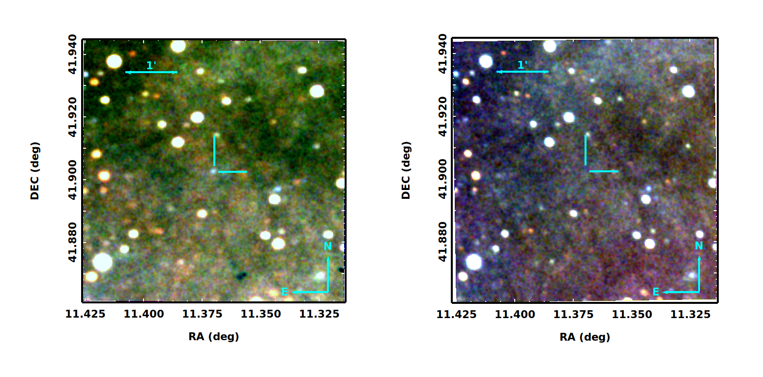
Figure 1: GIT RGB images of the M31N 2008-12a field during eruption (left) and in quiescence (right).

Nova eruptions are a consequence of thermonuclear runaway on the surface of a white dwarf (WD) primary in cataclysmic binary systems, resulting in the ejection of material in the range of $\rm~{}10^{-7}~{}-~{}10^{-4}~{}M_{\odot}$ (Gehrz et al. (1998); Hernanz & Jose (1998) and Starrfield (1999)). Inherently, all novae are supposed to be recurrent, with the primary WD and the secondary red-giant/sub-giant star sustaining all the eruptions. The observed recurrence period of novae can range from 1 year (M31N 2008-12a; Darnley et al. (2014)) to 98 years (V2487 Ophiuchi; Schaefer (2010)).

M31N 2008-12a (Figure 1) is an extraordinary RN whose eruptions have been observed every year in 2008–2022 (Table 1). It was first discovered during its 2008 eruption by Nishiyama & Kabashima (2008), though previous eruptions in 1992, 1993 and 2001 have been retrieved from the archives. Since the 2013 eruption, it has been monitored and studied across different wavelength ranges to understand its short recurrence period (2013 eruption – Darnley et al. 2014; Henze et al. 2014a; Tang et al. 2014; 2014 – Darnley et al. 2015c; Henze et al. 2015b; 2015 – Darnley et al. 2016, 2017b, 2017c; 2016 – Henze et al. 2018e).

The optical light curve and spectral evolution of this very fast RN were found to be similar during all the eruptions, with Balmer, He, and N lines dominating the spectrum. Light curves showed an extremely rapid rise to maximum ($\sim 1$ day) followed by a fast linear decline for about 4 days and a plateau with slow decline and jitters from day 4 to 8. The multi-eruption UV light curves were similar, with an initial rapid linear decline followed by slow plateau-like declines. The plateau phase coincided with the supersoft X-ray source (SSS) phase. Like optical and UV light curves, the SSS phase was similar during multiple eruptions.

The 2016 eruption (Henze et al., 2018e), however, deviated from the general trend. It occurred after a longer inter-eruption gap, the optical light curve showed a short-lived cuspy feature, and the UV and X-ray fluxes disappeared relatively early compared to the previous eruptions. The “peculiar” behaviour of the 2016 eruption was suggested to be due to a lower accretion rate prior to the 2016 eruption.

Theoretical models generated to satisfy the short recurrence period and short turn-on time of the SSS phase have allowed constraining the mass of the WD to near the Chandrasekhar limit (Tang et al., 2014; Kato et al., 2014).

Deep H$\alpha$ and HST imaging revealed the presence of an elliptical ($134\times 90$ parsecs) super-remnant nebula around M31 N2008-12a (Darnley et al., 2015c, 2017c). The size and mass of the shell indicate that the system has been undergoing eruptions for $\sim 10^{6}$ years (Darnley et al., 2019c) and would likely do so for $\sim 2\times 10^{4}$ more years before the WD attains $\rm M_{Ch}$ (Darnley et al., 2017c).

This paper discusses the recurrence period and its implication on the accretion rate and the mass of the primary WD. Also reported are the optical photometric and spectroscopic observations during the $2017-2022$ eruptions, along with the evolution of UV and soft X-ray emission based on Swift archival data and observed AstroSat data. The behaviour of the RN M31N2008-12a during the $2017-2022$ eruptions is compared to that of the previous eruptions.

Table 1: All known eruption dates of M31N 2008-12a till 2022

Eruption date(a)	Discovery	SSS-on date(b)	Days since	Detection wavelength	References
(UT)	mag (Filter)	(UT)	last eruption	(Observatory)
(1992 Jan 28)	$\cdots$	1992 Feb 03	$\cdots$	X-ray (ROSAT)	1, 2
(1993 Jan 03)	$\cdots$	1993 Jan 09	341	X-ray (ROSAT)	1, 2
(2001 Aug 27)	$\cdots$	2001 Sep 02	$\cdots$	X-ray (Chandra)	2, 3
2008 Dec 25	$\cdots$	$\cdots$	$\cdots$	Visible (Miyaki-Argenteus)	4
2009 Dec 02	$\cdots$	$\cdots$	342	Visible (PTF)	5
2010 Nov 19	$\cdots$	$\cdots$	352	Visible (Miyaki-Argenteus)	2
2011 Oct 22.5	$\cdots$	$\cdots$	337.5	Visible (ISON-NM)	5-8
2012 Oct 18.7	$\cdots$	$<$ 2012 Nov 06.45	362.2	Visible (Miyaki-Argenteus)	8-11
2013 Nov 26.95 $\pm$ 0.25	18.9 (R)	$\leq$ 2013 Dec 03.03	403.5	Visible (iPTF); UV/X-ray (Swift)	5, 8, 11-14
2014 Oct 02.69 $\pm$ 0.21	18.86 ($r^{\prime}$)	2014 Oct 08.6 $\pm$ 0.5	309.8 $\pm$ 0.7	Visible (LT); UV/X-ray (Swift)	8, 15
2015 Aug 28.28 $\pm$ 0.12	19.09 ($r^{\prime}$)	2015 Sep 02.9 $\pm$ 0.7	329.6 $\pm$ 0.3	Visible (LCO); UV/X-ray (Swift)	14, 16-18
2016 Dec 12.32 $\pm$ 0.17	17.62 (V)	2016 Dec 17.2 $\pm$ 1.1	471.7 $\pm$ 0.2	Visible (Itagaki); UV/X-ray (Swift)	19-23
2017 Dec 31.58 $\pm$ 0.20 †	18.41 (clear)	2018 Jan 05.6 $\pm$ 0.5	384.3 $\pm$ 0.4	Visible (WCO); UV/X-ray (Swift)	24-27
2018 Nov 06.67 $\pm$ 0.13 †	19.15	2018 Nov 13.2 $\pm$ 0.5	310.1 $\pm$ 0.3	Visible (LT); UV/X-ray (Swift)	28-31
2019 Nov 06.60 $\pm$ 0.11 †	19.40	2019 Nov 12.4 $\pm$ 0.5	364.9 $\pm$ 0.2	Visible (HO); UV/X-ray (Swift)	32-34
2020 Oct 30.49 $\pm$ 0.34 †	18.74 ($g^{\prime}$)	2020 Nov 05.5 $\pm$ 0.9	358.9 $\pm$ 0.4	Visible (LT); UV/X-ray (Swift)	35-38
2021 Nov 14.17 $\pm$ 0.21 †	18.7 (clear)	2021 Nov 19.2 $\pm$ 0.6	379.7 $\pm$ 0.5	Visible (Itagaki); UV/X-ray (Swift)	39-42
2022 Dec 02.50 $\pm$ 0.34 †	19.18 ($r^{\prime}$)	2022 Dec 07.5 $\pm$ 0.5	383.3 $\pm$ 0.5	Visible (LCOGT); UV/X-ray (Swift)	43-45

Notes: Updated version of Table 1 of Tang et al. 2014; Darnley et al. 2015c; Henze et al. 2015a; Darnley et al. 2016; Henze et al. 2018e.
^† Determined in this paper
^(a) Archival X-ray detections (cf., Henze et al. 2015a) are enclosed in brackets.
^(b) ROSAT data was used to estimate the SSS $\rm t_{on}$ for 1992 and 1993. The Chandra detection in 2001 Sep 08 UT has been taken to be the midpoint of a typical 12-day SSS phase to constraint eruption date.
$\cdots$ indicates unavailability of information.
References - (1) White et al. (1995), (2) Henze et al. (2015a), (3) Williams et al. (2004), (4) Nishiyama & Kabashima (2008), (5) Tang et al. (2014), (6) Korotkiy & Elenin (2011), (7) Barsukova et al. (2011), (8) Darnley et al. (2015c), (9) Nishiyama & Kabashima (2012), (10) Shafter et al. (2012), (11) Henze et al. (2014a), (12) Tang et al. (2013), (13) Darnley et al. (2014), (14) Darnley et al. (2016), (15) Henze et al. (2015b), (16) Darnley et al. (2015a), (17) Darnley et al. (2015b), (18) Henze et al. (2015c), (19) Henze et al. (2018e), (20) K. (2016), (21) Itagaki et al. (2016), (22) Henze et al. (2016a), (23) Henze et al. (2016b), (24) Boyd et al. (2017), (25) Henze et al. (2018b), (26) Henze et al. (2018c), (27) Naito et al. (2018a), (28) Henze et al. (2018a), (29) Darnley et al. (2018b), (30) Tan & Gao (2018), (31) Henze et al. (2018d), (32) Darnley et al. (2019a), (33) Oksanen et al. (2019), (34) Darnley et al. (2019b), (35) Galloway et al. (2020), (36) Darnley et al. (2020b), (37) Darnley & Page (2020), (38) Darnley et al. (2020a), (39) Itagaki et al. (2021), (40) Tan et al. (2021), (41) Darnley & Pag (2021a), (42) Darnley & Pag (2021b), (43) Perez-Fournon et al. (2022), (44) Shafter et al. (2022), (45) Darnley et al. (2022)

2 Observations

2.1 Optical

Table 2: Optical photometric observations of 2018–2022 eruptions of M31N 2008-12a. This is an example table. The full table will be made available in the online format

Date (UT)	Telescope	Filter	Magnitude
2018 Nov 07.58	JCBT	$B$	19.29 $\pm$ 0.28
2018 Nov 07.57	JCBT	$V$	18.78 $\pm$ 0.10
2018 Nov 08.57	HCT	$V$	19.27 $\pm$ 0.13
2018 Nov 08.56	HCT	$R$	19.11 $\pm$ 0.11
2018 Nov 08.55	HCT	$I$	18.83 $\pm$ 0.20
2018 Nov 08.76	GIT	$g^{\prime}$	19.60 $\pm$ 0.10
2018 Nov 08.77	GIT	$r^{\prime}$	19.15 $\pm$ 0.09
2018 Nov 08.74	GIT	$i^{\prime}$	19.28 $\pm$ 0.15

Photometric and spectroscopic observations were carried out using the following telescopes and instruments. The log of optical photometric observations is given in Table 2.

2.1.1 GROWTH-India Telescope

The GROWTH-India Telescope (GIT; Kumar et al. 2022 ) is a 0.7 m fully robotic telescope at the Indian Astronomical Observatory (IAO), Hanle, India. The telescope is equipped with a 4096 $\times$ 4108 Andor iKon-XL CCD. The detector has an image scale of 0.67^′′ pixel^-1 with a field of view (FoV) of 0.7^∘.

The GIT images were pre-processed, i.e., bias subtracted, flat-fielded and cosmic-ray corrected by the automated pipeline of the GIT (Kumar et al., 2022). Multiple exposures were obtained every night and in the case of low SNR, images from the same night and same filter were stacked using SWarp (Bertin et al., 2002).

For the 2018 data, aperture photometry was performed using an aperture of $\sim 2.5^{\prime\prime}$, close to the full-width half maximum (FWHM) of the stellar profile in the images. For 2020–2022 data, the FWHM was first calculated using SExtractor (Bertin & Arnouts, 1996) and subsequently used in Image Reduction and Analysis Facility (IRAF , Tody (1993)) to perform PSF photometry. The magnitudes of the local standard stars given in Darnley et al. (2016) were converted from $BVRI$ to $gri$ using the transformations in Jester et al. (2005) to determine the zero points for photometric calibrations.

2.1.2 Himalayan Chandra Telescope

The Himalayan Faint Object Spectrograph Camera (HFOSC) mounted on the 2 m Himalayan Chandra Telescope (HCT) located at IAO, Hanle, India was used to obtain images in the $VRI$ bands on 2018 Nov 08 UT. HFOSC is equipped with a 2K $\times$ 4K CCD. The pixels correspond to an image scale of 0.296^′′ pixel^-1, with a FoV of $10^{\prime}~{}\times~{}10^{\prime}$ for the central 2K $\times$ 2K region. The images were pre-processed using the standard routines in IRAF. The instrumental magnitudes were obtained using aperture photometry with an aperture set at a radius three times the FWHM. Differential photometry was performed with respect to the local standards (Darnley et al., 2016) to account for the zero points of the images.

Optical spectra were obtained using HFOSC on 2018 Nov 07.8 and 08.6 UT (Pavana et al., 2018), 2019 Nov 07.5 UT, 2020 Oct 31.6 UT, 2021 Nov 14.8 and 15.6 UT (Sonith et al., 2021), and 2022 Dec 03.7 and 04.5 UT (Basu et al., 2022). We used a grism (Gr7) with R $\approx$ 1200 in the wavelength range of 3500 - 7800 Å. Data reduction was performed in the standard manner using IRAF. All the spectra were bias subtracted, cosmic-ray corrected and extracted. Wavelength calibration was carried out using the FeAr arc lamp spectrum. Spectro-photometric standard stars were used to correct the instrumental response and bring the spectra to a relative flux scale. Absolute flux calibration was done based on zero points obtained from broadband magnitudes.

2.1.3 J.C. Bhattacharyya Telescope

The 2K $\times$ 4K UK Astronomy Technology Centre (UKATC) CCD mounted on the 1.3 m Jagadish Chandra Bhattacharya Telescope (JCBT), located at the Vainu Bappu Observatory (VBO), Kavalur, India, was used during the 2018 eruption. It has a 15-micron pixel size corresponding to an image scale of 0.3^′′ pixel^-1, with a FoV of $10^{\prime}\times 20^{\prime}$. JCBT observed the nova in $BV$ bands 2 days after the eruption. The images were reduced and calibrated following the same steps used for HCT data.

2.1.4 Other data sources

Our observations were combined with publicly available photometric data for analysis, from sources referenced below.

• 2017: Socia et al. (2018); Hornoch et al. (2018); Kaur et al. (2018b, c); Naito et al. (2018b); Kaur et al. (2018a); Erdman et al. (2018); Darnley et al. (2018a).

• 2018: Engesser et al. (2018); Agnihotri & Raj (2018a); Wysocki et al. (2018); Tan & Gao (2018); Agnihotri & Raj (2018b); Kaur et al. (2018d); Zwicky Transient Facility (ZTF) archive (ALeRCE Explorer , Förster et al. 2021).

• 2019: Hornoch et al. (2019); Horst et al. (2019); Kaur et al. (2019); ZTF archive.

• 2020: Perez-Fournon et al. (2020); Galloway et al. (2020); Rajagopal et al. (2020).

• 2021: Taguchi et al. (2021); Naito et al. (2021)

• 2022: Rodriguez et al. (2023); Shafter et al. (2022); Agnihotri et al. (2022); Tan et al. (2022); Erdman et al. (2022).

2.2 Ultraviolet

Table 3: AstroSat (UVIT and SXT) and Swift (UVOT and XRT) observations of $2017-2022$ eruptions of the M31N 2008-12a. The complete table will be made available in online format.

Obs ID	Date (UT)	UV mag (AB)	Count rate ($\times 10^{-3}$ count s-1)
AstroSat		UVIT F148W	SXT $(0.3-2.0)$ keV
T03_156T01_9000003312	2019-11-19.78	23.03 $\pm$ 0.14	–
T03_259T01_9000003972	2020-11-03.25	21.30 $\pm$ 0.09	–
T03_262T01_9000003988	2020-11-10.76	22.78 $\pm$ 0.12	25.81 $\pm$ 2.18
	2020-11-11.09		34.33$\pm$ 2.68
	2020-11-11.42		31.30 $\pm$ 2.18
	2020-11-11.75		32.03 $\pm$ 2.52
	2020-11-12.09		32.94 $\pm$ 2.22
	2020-11-12.42		32.11 $\pm$ 2.14
	2020-11-12.75		45.70 $\pm$ 17.31
T04_066T01_9000004772	2021-11-18.97	21.25 $\pm$ 0.12	–
T04_072T01_9000004780	2021-11-23.22	22.96 $\pm$ 0.09	23.63 $\pm$ 3.06
	2021-11-23.41		31.22 $\pm$ 2.31
	2021-11-23.74		26.20 $\pm$ 2.35
	2021-11-24.07		31.83 $\pm$ 3.27
	2021-11-24.41		31.79 $\pm$ 2.36
	2021-11-24.74		34.09 $\pm$ 2.72
	2021-11-25.07		24.02 $\pm$ 3.39
T05_058T01_9000005414	2022-12-07.23	21.38 $\pm$ 0.07	–
Swift		UVOT uvw2	XRT $(0.3-1.5)$ keV
00010498001	2018-01-01.22	18.87 $\pm$ 0.05	$<39.4$
00010498002	2018-01-02.36	19.59 $\pm$ 0.06	$<38.1$
00010498003	2018-01-03.81	20.76 $\pm$ 0.16	$<55.9$
00010498004	2018-01-04.49	20.27 $\pm$ 0.09	$<30.2$
00010498005	2018-01-05.48	20.69 $\pm$ 0.06	3.6 $\pm$ 1.0
00010498006	2018-01-05.94	20.90 $\pm$ 0.07	11.8 $\pm$ 1.6
00010498007	2018-01-07.14	21.10 $\pm$ 0.08	12.1 $\pm$ 1.7
00010498008	2018-01-08.07	21.00 $\pm$ 0.08	13.8 $\pm$ 2.0

Photometric studies were done using images obtained in the ultraviolet (UV) bands from the following two telescopes.

2.2.1 Swift UVOT

High cadence UV imaging data of M31N 2008-12a are available from the Swift (Gehrels et al., 2004) archive . The nova has been monitored by UVOT since 2013 during each eruption. The log of Swift observations during $2017-2022$ are summarised in Table 3. We have used the uvw2 (1928$\pm$657 Å) archival data in this study. The uvot task in HEASOFT (v6.29) was used to extract the magnitudes from a source region of radius 5^′′ after background subtraction. The calibration assumes the UVOT photometric (AB) system (Poole et al. 2008 and Breeveld et al. 2011) and is not corrected for extinction.

2.2.2 AstroSat UVIT

AstroSat (Singh et al., 2014) is a space-based telescope with the Ultraviolet Imaging Telescope (UVIT) as one of its instruments. UVIT observed M31N 2008-12a during its $2019-2022$ eruptions in F148W (1481$\pm$500 Å) filter (see Table 3). The level 1 UVIT data was downloaded from the Indian Space Science Data Center (ISSDC) and reduced using CCDLAB following standard routines presented in Postma & Leahy (2021). The orbit-wise images were registered and merged to obtain a single image with a high SNR on which astrometry was performed. The average PSF size in UVIT images was $\sim 1.5^{\prime\prime}$ across all epochs. We performed PSF photometry with an aperture correction term derived from “good stars” to account for the broad PSF wings in UVIT images. The zero points for photometric calibrations in the AB system were adopted from Tandon et al. (2020) and have not been corrected for extinction.

2.3 X-ray

Both Swift and AstroSat observe simultaneously in the UV and X-ray wavelengths. Soft X-ray observations from both facilities were used to study the eruptions during the SSS phase.

2.3.1 Swift XRT

Swift X-Ray Telescope (XRT; Burrows et al., 2005) data were downloaded from the Swift archive, with Observation IDs same as that of the UVOT data (Table 3). For the analysis, HEASOFT (v6.29) with XIMAGE (v4.5.1) and XSELECT (v2.5b) were used following the guidelines summarised by UKSSDC. XRT count rates were determined using XIMAGE sosta tool with the optimize command, which corrects the counts for vignetting, dead time loss, background subtraction and the PSF. We used XSELECT to extract the spectra for each snapshot. ARF files were generated from the exposure maps, while RMF files were taken from the calibration database. Spectral analysis was performed in XSPEC (v12.12.0) assuming Poisson statistics (cstat) due to low counts. We used ISM abundances given in Wilms et al. (2000) and the Tübingen–Boulder (tbabs) ISM absorption model to account for the intervening medium.

2.3.2 AstroSat SXT

AstroSat Soft X-ray telescope SXT (Singh et al., 2017), placed in parallel alongside UVIT, is capable of observing in the $\rm 0.3~{}-~{}8.0~{}keV$ range simultaneously with UVIT (Table 3). SXT observed the SSS phase of M31N 2008-12a during the 2020 and 2021 eruptions. Level 2 data was downloaded from ISSDC, and the cleaned event files were merged using SXTTools in Julia. The source region was chosen as a circle of radius $7^{\prime}$, smaller than the usual SXT PSF of $\sim 12^{\prime}$ so to avoid contamination in the crowded M31 field. We set the bin size to 8 hours and energy range to $0.3-2.0$ keV in XSELECT to attain an adequate SNR for light curve analysis. SXT spectra were extracted using XSPEC from the merged SXT cleaned event files. A new ARF file was generated corresponding to the smaller source extraction region for analysis.

2.4 Epoch of eruptions

For a very fast RNe, like M31N 2008-12a, a tight constraint on the eruption time is useful for generating light curve models (§4.3) and studying its recurrence nature (§3). Hence, we estimate the epochs of eruption based on available detection and pre-discovery magnitudes and non-detection upper limits for all eruptions since 2017. Even though the exact time of eruption is uncertain, it can be well approximated by the mid-point of first detection and last non-detection in each year. Amateur astronomers’ interest in M31 and the increase in survey telescopes over the past decade have made it possible to constrain the eruption date to well within a day. The uncertainty in the eruption dates spans between the first detection and the last non-detection.

The 2017 eruption was discovered just in time to be called the “2017 eruption” on Dec 31.77 UT by Boyd et al. (2017). Darnley et al. (2017a) reported spectroscopic confirmations on the same day. The last non-detection was on Dec 31.38 UT at an upper limit of $\rm m_{clear}=19~{}mags$ (Naito et al., 2018a).

The 2018 eruption was discovered on Nov 06.80 UT at a magnitude of $19.15\pm 0.05$ by Darnley et al. (2018b) and confirmed spectroscopically by Darnley et al. (2018c) on the same day. Tan & Gao (2018) reported the last non-detection at $>21.20$ mag on Nov 06.54 UT in clear filter.

The 2019 eruption was detected on Nov 06.71 UT by Oksanen et al. (2019) at 19.40 mags. The first spectrum taken on Nov 06.83 UT (Darnley et al., 2019d) confirmed the recurrence of M31N 2008-12a. The last non-detection information was not publicly available for 2019, so we adopted the eruption date provided in Darnley et al. (2019b).

Darnley et al. (2020b) discovered the 2020 eruption on Oct 30.89 UT. The nova was, however, also detected in images captured 90 minutes before the discovery (Galloway et al., 2020), and we use the pre-discovery detection ($\rm m_{g}=18.74$) and non-detection ($\rm m_{g}>19.4$) to constrain the eruption time. The discovery was spectroscopically confirmed on the next day (Darnley, 2020).

The 2021 eruption was discovered on Nov 14.38 UT by Itagaki et al. (2021) and was spectroscopically confirmed by Wagner et al. (2021). Tan et al. (2021) gave pre-detection upper-limits at $\rm m_{clear}>19.00~{}mags$ on Nov 13.96 UT.

The 2022 eruption was discovered on Dec 2.83 UT by Perez-Fournon et al. (2022). It was undetected until Dec 02.61 UT at $\rm m_{L}>19.60~{}mags$ (Shafter et al., 2022). Spectra taken on Dec 3.84 UT confirmed the source to be a recurrence of the nova (Darnley & Healy, 2022), its 15th successive eruption in as many years.

The estimated eruption dates for the years 2017-2022 are presented in Table 1 together with those of the previous ones.

3 Recurrence period, Accretion rate and WD mass

M31N 2008-12a has erupted every year since 2008, making it an exceptional case of the only RN observed 15 times and that too consecutively. This section focuses on the trend of the recurrence period and its relation to the accretion rate and the WD mass.

3.1 Increasing recurrence period

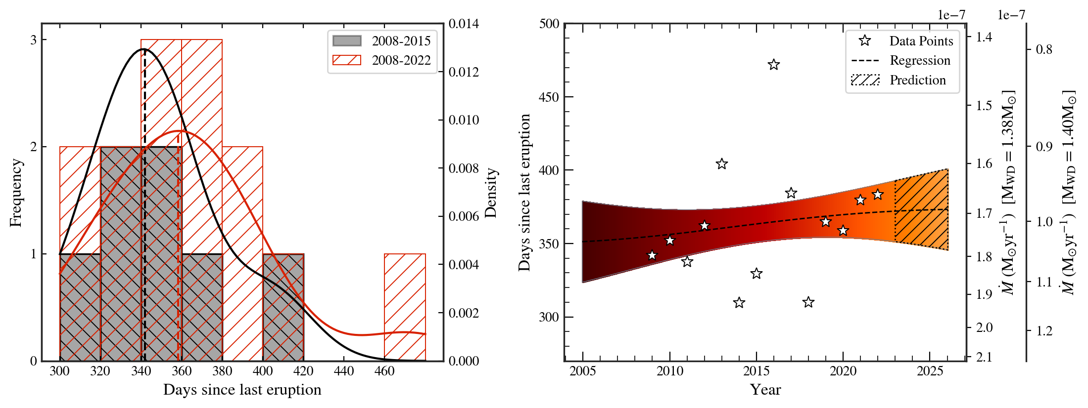
Figure 2: Left: Distribution of the frequency of eruptions as a function of days since the last eruption binned at 20 days. Grey histogram is for $2008-2015$ eruption data, and black solid line represents the KDE for this data. Red histogram and red solid line represents the same for $2008-2022$ data. Right: Eruptions marked with stars. Dashed line and coloured area represent the mean function and 3$\sigma$ error function of the GP regression tracking the recurrence period with time. Shaded region is our prediction for the $2023-2025$ eruptions, given we don’t see outlier events. Y-axes on the RHS represent the accretion rates for $\rm 1.38~{}M_{\odot}$ and $\rm 1.40~{}M_{\odot}$ WD corresponding to the recurrence period on the primary y-axis.

The mean recurrence period was reported to be $\rm P_{\text{rec}}~{}=~{}351\pm~{}13$ days after the 2015 eruption by Darnley et al. (2016), which was updated to $363\pm 52$ days after the outlier 2016 event by Henze et al. (2018e). Since the 2016 eruption, M31N 2008-12a erupted six more times, and each year, the time gap between two successive eruptions has been more than the mean recurrence period except in 2018 (310.1 days) and 2020 (355.9 days). As of the 2022 eruption, the mean recurrence period is $\rm P_{\text{rec}}=363.6$ days with a standard deviation of 40.3 days. On the other hand, the median recurrence period has increased from 347 days in 2016 (Henze et al., 2018e) to 360.5 days in 2022. Figure 2 shows two different sets of histograms, along with their kernel density estimates (KDE), for the recurrence periods between $2008-2015$ and $2008-2022$. On considering up to the 2015 eruption (grey histogram in Figure 2), the mode of the recurrence period is 340 days and the KDE peaks at 341.28 days (FWHM of 67.27 days). But on incorporating all the eruption information till 2022 (red histogram in Figure 2), the mode of recurrence period shifts to 360 days with the KDE peaking at 358.18 days (FWHM of 96.36 days). We see a clear increasing trend of the recurrence period over the last 7 years.

To further investigate this matter, we plotted the period as a function of the eruption year in the right panel of Figure 2. We used the GP regression technique to extract the trend in the data set and associate errors with it. The data was modelled using a Matern kernel with a typical length scale of 15 years and an amplitude equal to the median of the recurrence period. We tested our model by applying it to the eruption dates of $2008-2021$, and it could predict the 2022 eruption date within $3\sigma$ error limits. The 2022 data was subsequently included in the training set to predict the upcoming eruptions in $2023-2025$. The $3\sigma$ upper and lower ranges of the recurrence period from our model predictions are

• 2023: $\rm 18~{}Nov~{}2023-30~{}Dec~{}2023$

• 2024: $\rm 23~{}Nov~{}2024-08~{}Jan~{}2025$

• 2025: $\rm 28~{}Nov~{}2025-18~{}Jan~{}2026$

The predicted recurrence period for the next three eruptions is around 372.5 days, which is more than the mean, median, and mode of recurrence period ($\sim 360$ days) obtained for all previous eruptions. Here, we point out that our model is restricted to predicting only the ‘usual’ eruptions that follow the trend. The prediction of ‘outlier’ events, such as the 2016 eruption, is not guaranteed.

3.2 Estimating the WD mass

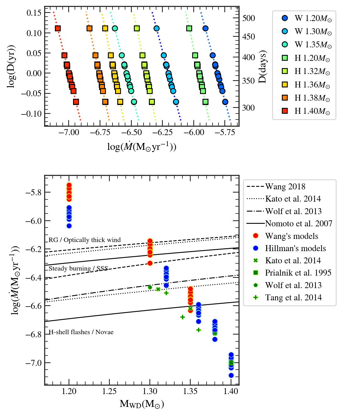
Figure 3: Top: Observed recurrence period plotted against accretion rate different WD masses. “W” and “H” in the legend indicate accretion rates derived from Wang (2018) and Hillman et al. (2016) respectively. Bottom: $\rm M_{WD}-$$\dot{M}$ parameter space for M31N 2008-12a. Accretion rates from the top panel are shown in red (Wang’s) and blue (Hillman’s). Overplotted in green markers are for the one-year recurrence period taken from the literature. Stable and critical accretion rate limits from four studies are shown as horizontal tracks.

In a theoretical study to understand the possible mass growth of a WD accreting matter from a non-degenerate companion, Hillman et al. (2016) have explored a range of accretion rates and derived limits on the accretion rate and on the initial mass that will allow a WD to reach the Chandrasekhar limit. Adopting their relation between $D$ (period) and $\dot{M}$ (accretion rate) for hydrogen accretion cases, $\log~{}\dot{M}~{}=~{}\rm-A~{}\log~{}D~{}-~{}B$, we estimate the accretion rates in the last 15 years for the M31 RN eruptions. Here, the coefficients A and B depend on the WD mass. For each value of $\rm M_{WD}$, A and B were determined by fitting a linear function to the parameter space of $\rm\log~{}D$ and $\log~{}\dot{M}$. The accretion rates of WD masses between $\rm 1.20~{}M_{\odot}$ and $\rm 1.40~{}M_{\odot}$ corresponding to the periods of M31N 2008-12a are shown in the top panel of Figure 3.

Wang (2018) have used the Modules for Experiments in Stellar Astrophysics (MESA) to model the binary evolution of WD accreting H-rich material from a companion for a range of WD masses and accretion rates. The composition of the accreted material was fixed at H:He:Metals $\equiv$ 70:28:2. We use their results for the massive WD cases ($\rm 1.20-1.35~{}M_{\odot}$), obtain a best-fit power-law relation between the accretion rate and the period and employ the same to infer the accretion rates for each cycle of M31N 2008-12a. These are also shown in the top panel of Figure 3.

We plot the accretion rates thus obtained corresponding to the periods of M31N 2008-12a in the last 15 years in the $\rm M_{WD}-$$\dot{M}$ parameter space in the bottom panel of Figure 3. For comparison, we over-plot the results from Kato et al. (2014), Prialnik & Kovetz (1995), Wolf et al. (2013), and Tang et al. (2014), who predicted the WD mass and accretion rates for a recurrence period of 1 year.

In the $\rm M_{WD}-$$\dot{M}$ plane, when the accretion rate surpasses the critical threshold ($\dot{M}~{}>~{}\dot{M}\rm_{cr}$), the WD exhibits a red giant (RG) like behaviour, undergoing surface mass burning at the critical rate, while any excess material is ejected in the form of optically thick winds (Kato & Hachisu, 1994; Hachisu et al., 1996). Conversely, when the accretion rate falls below the critical threshold but remains above the stable H accretion rate, i.e. $\dot{M}\rm_{cr}$ $~{}>~{}\dot{M}~{}>$ $\dot{M}\rm_{st}$, the burning on the WD’s surface remains stable, capable of sustaining itself over an extended period as a supersoft X-ray emitter (Kato et al., 2014). Below the stability line, i.e. $\dot{M}\rm_{st}$$>\dot{M}$, the accretion rate is insufficient to sustain continuous hydrogen burning. Systems within this parameter range experience ”H-shell flashes” or nova eruptions, a category that includes all RNe, including M31N 2008-12a.

The limits on $\dot{M}\rm_{cr}$ and $\dot{M}\rm_{st}$ taken from Wang (2018), Kato et al. (2014), Wolf et al. (2013), and Nomoto et al. (2007) are shown in the bottom panel of Figure 3. The differences in these limits are primarily because of the different techniques employed in modelling.

We infer from Figure 3 (bottom panel) that a WD with mass below 1.30 $\rm M_{\odot}$ has a high accretion rate and does not allow the RN phenomenon to occur at the rate of once a year.

We also see that $1.32-1.36~{}\rm M_{\odot}$ WDs do fall into the “H-shell flash” region of some of the models, and any WD with $\rm M_{WD}~{}>~{}1.36~{}M_{\odot}$ satisfies the necessary criteria of nova eruption ($\dot{M}$$<\dot{M}\rm_{st}$) for all the models. Thus, the WD mass in M31N 2008-12a is likely to be greater than $\rm 1.36~{}M_{\odot}$, which would in turn allow “H-flash” features at the observed recurrence period of M31N 2008-12a.

4 UV and optical light curve

4.1 Light curve evolution

The optical light curves of the $2017-2022$ eruptions, based on our observations and publicly available data, are shown in Figure 4. The light curves indicate a rapid rise to the peak magnitude in $<1$ day from discovery, followed by a fast decline with $t_{2}\approx 2-4$ days in $g^{\prime}r^{\prime}i^{\prime}$ bands. A brief description of the optical light curve for each eruption during $2017-2022$ is provided below.

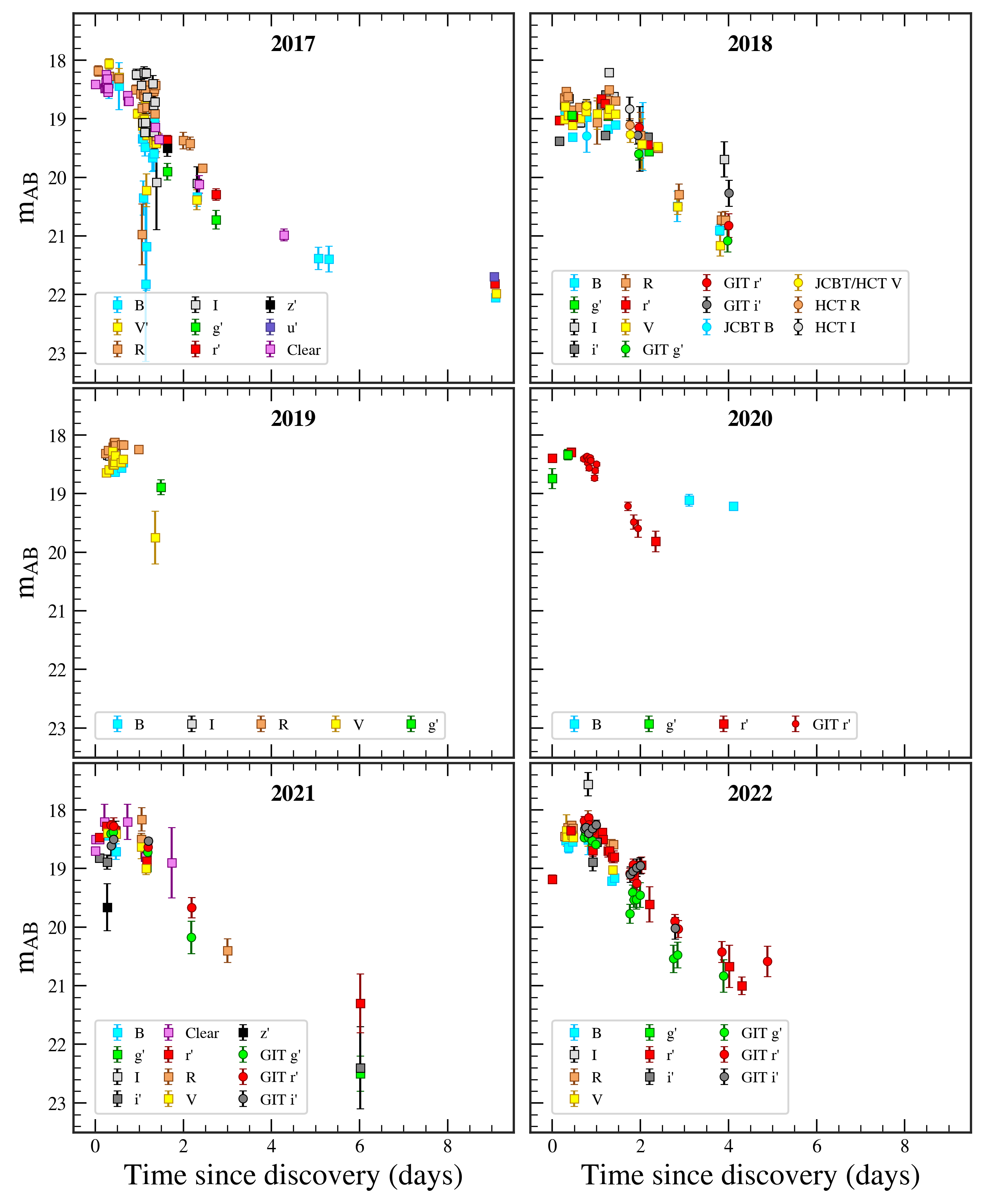
Figure 4: Optical light curves of M31N 2008-12a for $2017-2022$ eruptions. GIT, HCT, and JCBT observations are plotted with publicly available data.

The 2017 light curves show a rapid decline in the first 4 days, followed by a slow decline in all the bands. The decline rate is marginally faster in the $r^{\prime}$ band ($\rm 0.84\pm 0.12~{}mag~{}day^{-1}$) compared to the $g^{\prime}$ band ($\rm 0.74\pm 0.19~{}mag~{}day^{-1}$). However, the decline rates in $g^{\prime}$ and $r^{\prime}$ were measured using only two data points and are within error bars of each other.

The maximum phase during the 2018 eruption appears to be broader. Following the initial rise, the magnitude declined by $\sim~{}0.4$ mag in the $BVRI$ filters, and after a brief halt for about 0.3 days at this level, a marginal increase in the brightness by $0.2-0.3$ mag lasting $\sim 0.7$ days can be seen. We also note that the peak magnitude observed in 2018 in $R$ (18.50 mag) is fainter than the peak $R$ or $r$ magnitudes in the other years. In 2018, the initial decline in the $r^{\prime}$ ($\rm 0.68\pm 0.03~{}mag~{}day^{-1}$) and $i^{\prime}$ ($\rm 0.53\pm 0.04~{}mag~{}day^{-1}$) bands was slower by $0.1-0.2$ mag per day compared to other years. Further, the decline rates of $r^{\prime}$ and $i^{\prime}$ are slower than $g^{\prime}$ band ($\rm 0.84\pm 0.02~{}mag~{}day^{-1}$) in 2018.

The 2019 data set is sparse and restricted to the initial rise and maximum phases. The nova is brighter in $R$ compared to $BV$ bands during the rise and the peak. It rises about 0.4 mag in all the bands in about 0.5 days from discovery. The peak $R$ magnitude reached in 2019 is $\rm m_{R}=18.12$, which is higher than most other eruptions.

The $g^{\prime}$ band traces the rise of the 2020 light curve at $\rm\sim 1.2~{}mag~{}day^{-1}$ while the $r^{\prime}$ band traces the smooth decline from the peak at $\rm 0.89\pm 0.05~{}mag~{}day^{-1}$ for 2 days. Limited data only restricts the light curve analysis to the $r^{\prime}$ band.

The 2021 eruption was caught almost a day before it reached its peak. The rise was sharper in the $i^{\prime}$ band compared to the $g^{\prime}r^{\prime}$ bands. It declined rapidly in the $g^{\prime}$ band at $\rm 1.25\pm 0.20~{}mag~{}day^{-1}$ but relatively slowly in the $r^{\prime}$ band at $\rm 0.88\pm 0.13~{}mag~{}day^{-1}$ for the first $\rm 3-4~{}days$. The decline rate then slowed with significant enhancement in the $r^{\prime}$ band flux around 6 days after the eruption.

The 2022 eruption light curve was similar to previous years. The rise is well captured in the $r^{\prime}$ band with a rate of $\sim$ 2 mag day^-1, the fastest in the last six years. It then declined speedily in the $g^{\prime}$ band ($\rm 1.01~{}\pm~{}0.05~{}mag~{}day^{-1}$) but relatively slowly in $r^{\prime}$ band ($\rm 0.79~{}\pm~{}0.03~{}mag~{}day^{-1}$) and even more slowly in the $i^{\prime}$ band ($\rm 0.69\pm 0.06~{}mag~{}day^{-1}$).

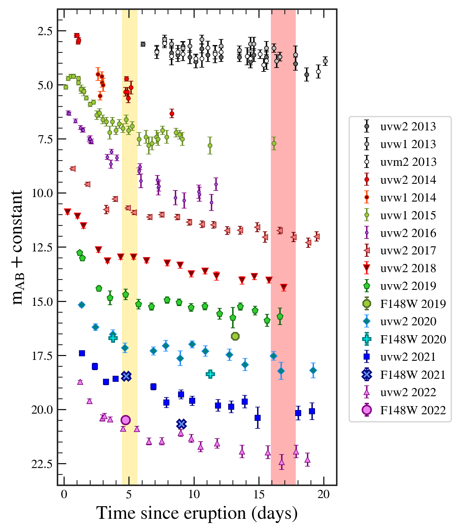
Figure 5: UVOT light curves of M31N 2008-12a shown for $2013-2022$ eruptions. UVIT F148W data are overplotted. SSS $\rm t_{on}$ and $\rm t_{off}$ times are highlighted in yellow and red respectively.

Generally, the nova declines fastest in the $g^{\prime}$ band and comparatively slower in the redder bands. Darnley et al. (2016) combined the 2013, 2014, and 2015 eruptions and found the decline rate to be fastest in the $V$ band at $1.21~{}mag~{}day^{-1}$ during the initial decline phase. The evolution of the optical light curve during the later phases is unavailable as the nova fades beyond the detection limit of the $1-2~{}m$ class ground-based telescopes generally used for follow-up observations.

The UV light curves (Figure 5) obtained from space-based telescopes have a wider time coverage ($\sim$ 20 days) and show a linear decline in the $2017-2022$ $uvw2$ magnitudes from day 0 to 3 since the eruption. The plateau phase begins with a re-brightening at $\sim~{}4$ days since the eruption, which is also coincident with the SSS turn-on time (yellow shaded region in Figure 5). The evolution during this phase indicates a gradual decline $\sim$ 0.15 mag day^-1 with several undulations or jitters on top of it. Strope et al. (2010) presented light curve samples of various classes of novae, and some of the P-type galactic recurrent novae, such as T Pyx, RS Oph and U Sco, do show such variability in the $V$-band during their plateau phase.

The F148W data show that during the initial decline phase, the brightness in the F148W filter is similar to $uvw2$ but becomes fainter by $>0.5$ mag than $uvw2$ during the SSS phase.

The general trends across all the UV–optical bands in $2017-2022$ eruptions are more or less similar over the last six years and consistent with the previous eruptions (2013: Darnley et al. 2014, 2014: Darnley et al. 2015c, 2015: Darnley et al. 2016, 2016: Henze et al. 2018e). However, some deviations of the 2016 light curve were noted and discussed in §7.

4.2 Colour Evolution

The (F148W$-uvw2$) colour was determined from observations taken on the same day. From Figure 6, it is seen that the (F148W$-uvw2$) colour becomes bluer at the onset of the SSS phase but is significantly redder during the SSS phase.

In the optical bands, we restrict the colour analysis to only the SDSS primed filters to avoid instrumental and/or filter dependencies of the Bessel filters. Near-simultaneous observations in $g^{\prime}r^{\prime}$ and $r^{\prime}i^{\prime}$ filters for the same eruption were used to estimate the colours. The colours are plotted together as a function of days since the eruption to bring all the outbursts to the same time scale. The ($g^{\prime}-r^{\prime}$) colour linearly increases up to day 3 from the eruption and then decreases. This timeline agrees with the initial rise and linear decline phase of the light curve. The ($r^{\prime}-i^{\prime}$) colour shows a steep reddening during the rising phase, which then slows down as the nova follows its initial decline. After 3 days from the eruption, the ($g^{\prime}-r^{\prime}$) colour becomes bluer while the ($r^{\prime}-i^{\prime}$) colour also tends to be bluer, but due to only one data point between day 3 and day 4, we are unable to confirm this. Beyond day 4, the ($r^{\prime}-i^{\prime}$) colour becomes redder when the nova enters its plateau phase. A similar trend was also noted by Darnley et al. (2016) in their colour plots.

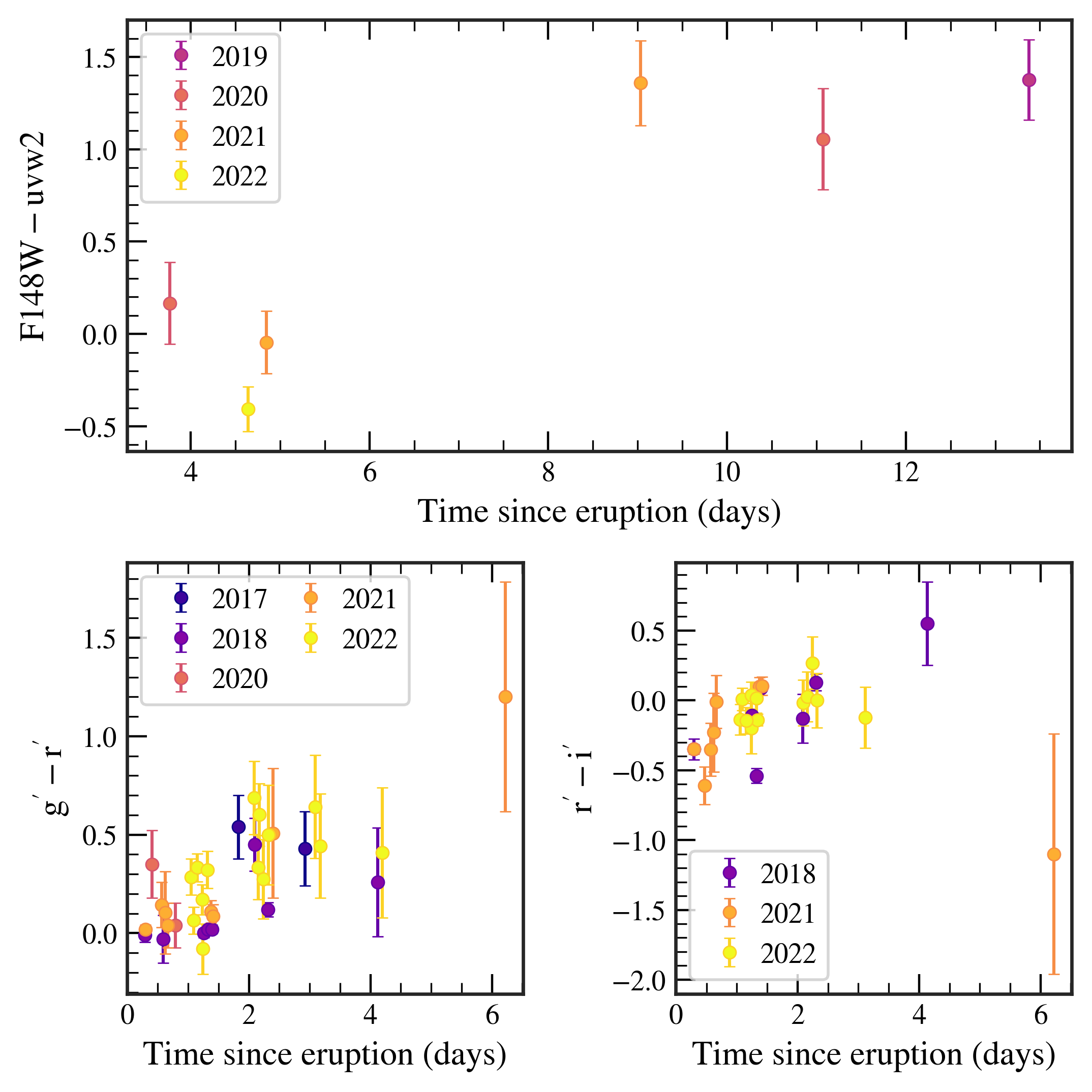
Figure 6: Colour evolution of M31N 2008-12a in UV and optical bands for $2017-2022$ eruptions.

4.3 Light curve modelling

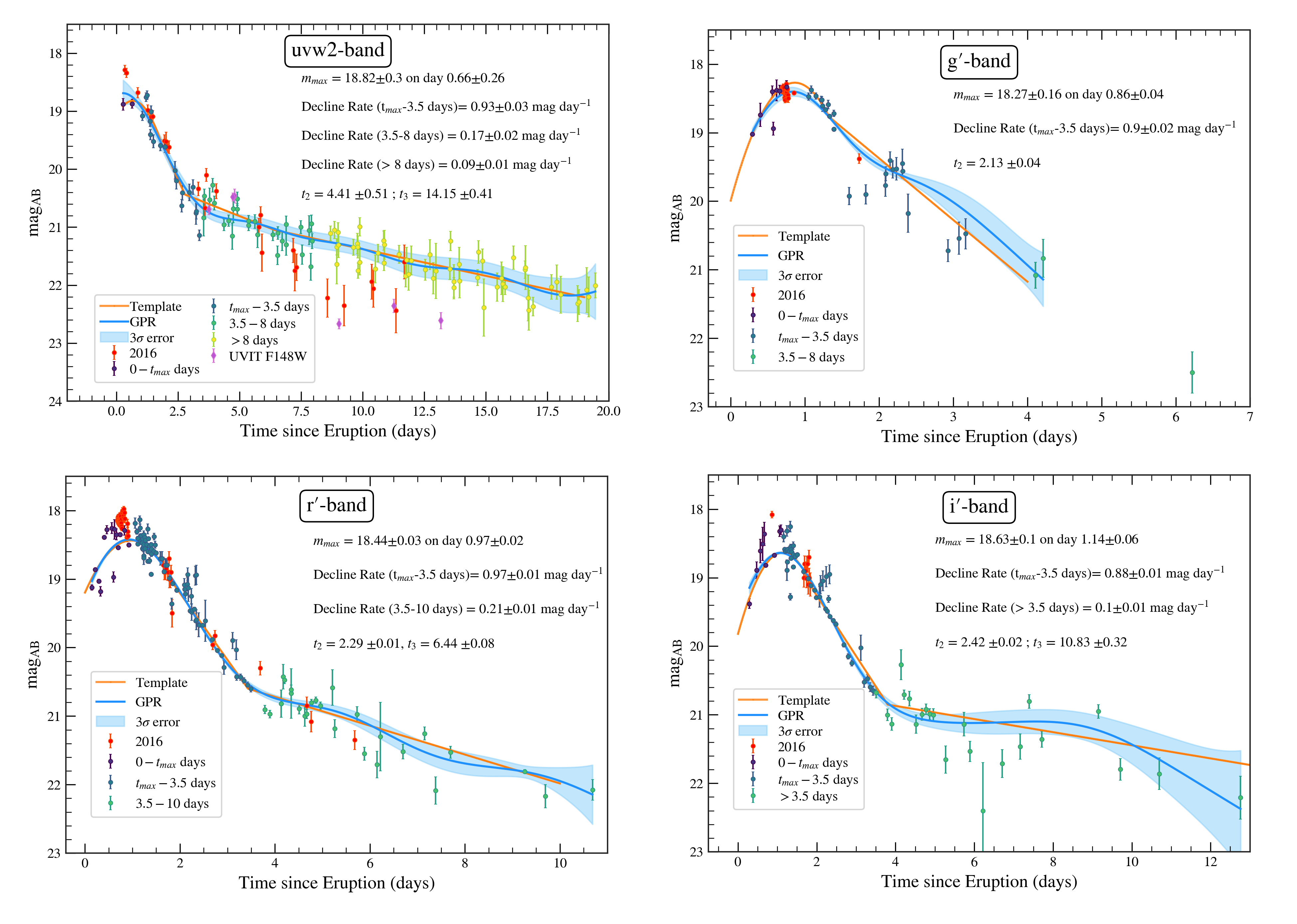
Figure 7: Light curve properties of 2013-2022 (except 2016) eruptions for $uvw2,g^{\prime},r^{\prime},$ and $i^{\prime}$ bands (clockwise from top-left). Outlier data points of 2016 are marked in red. The light curve template, in orange, was generated by stitching the phases in each filter. GP mean and $3\sigma$ error functions are shown in blue.

Table 4: Multi-eruption light curve model parameters

Filter	$\rm t_{max}^{a}$	$\rm m_{max}$	$\rm t_{2}$	$\rm t_{3}$	Decline Rates ($\rm mag~{}day^{-1}$)
	(days)	(AB)	(days)	(days)	$\rm t_{max}~{}to~{}3.5$	$\rm 3.5~{}to~{}\sim 8$	$>8$
$2017-2022$
uvw2	0.66 $\pm$ 0.26	18.82 $\pm$ 0.30	4.41 $\pm$ 0.51	14.15 $\pm$ 0.41	0.93 $\pm$ 0.03	0.17 $\pm$ 0.02	0.09 $\pm$ 0.01
g’	0.86 $\pm$ 0.04	18.27 $\pm$ 0.16	2.13 $\pm$ 0.04	$\cdots$	0.90 $\pm$ 0.02	$\cdots$	$\cdots$
r’	0.86 $\pm$ 0.09	18.21 $\pm$ 0.27	2.37 $\pm$ 0.05	5.87 $\pm$ 5.61	0.88 $\pm$ 0.02	0.19 $\pm$ 0.18	$\cdots$
i’	0.88 $\pm$ 0.12	18.30 $\pm$ 0.62	3.26 $\pm$ 0.20	$\cdots$	0.56 $\pm$ 0.04	$\cdots$	$\cdots$
$2013-2022$ (Excluding 2016)
uvw2	0.66 $\pm$ 0.26	18.82 $\pm$ 0.30	4.41 $\pm$ 0.51	14.15 $\pm$ 0.41	0.93 $\pm$ 0.03	0.17 $\pm$ 0.02	0.09 $\pm$ 0.01
g’	0.86 $\pm$ 0.04	18.27 $\pm$ 0.16	2.13 $\pm$ 0.04	$\cdots$	0.90 $\pm$ 0.02	$\cdots$	$\cdots$
r’	0.97 $\pm$ 0.02	18.44 $\pm$ 0.03	2.29 $\pm$ 0.01	6.44 $\pm$ 0.08	0.97 $\pm$ 0.01	0.21 $\pm$ 0.02	$\cdots$
i’	1.14 $\pm$ 0.06	18.63 $\pm$ 0.10	2.42 $\pm$ 0.02	10.83 $\pm$ 0.32	0.88 $\pm$ 0.01	0.10 $\pm$ 0.01	$\cdots$

^aDays since eruption

To understand the temporal evolution of the light curves, we model them by breaking them into three phases corresponding to different decline rates. The $uvw2,g^{\prime},r^{\prime},\text{ and }i^{\prime}$ band are used. The eruption times presented in Table 1 are used as the reference times, and we measure all other times in days with respect to the reference date of each eruption. The three phases considered are

1. The rise to peak: from eruption to $\rm t\approx 1.5$.

2. The initial steep decline: $\rm t_{max}\leq t\leq 3.5$, where $\rm t_{max}$ is the time of maxima

3. The slow decline: $\rm t\geq 3.5$

Due to extensive coverage in the uvw2 filter, we could notice that the rate of decline decreased even further beyond 8 days of eruption. The final phase is thus divided into two segments in $uvw2$. Darnley et al. (2016) employed a similar 4-phase division of all light curves to analyse previous eruptions.

First, we generated models for the combined $2017-2022$ eruptions and obtained the light curve properties at different phases given in Table 4. Then, we combined the $2013-2015$ eruptions’ data with those from $2017-2022$ and generated overall light curve models spanning from 2013 to 2022. We note here that the data in $g^{\prime}$ is sparse as it was not used in most of the observations before 2016. The 2016 data set has been intentionally excluded as an outlier as it deviated significantly from the general trend of other eruptions (plotted in red points in Figure 7), especially in the UV light curve. The combined light curve models are presented in Figure 7 and the light curve parameters are tabulated in Table 4.

Additionally, Gaussian process (GP) regression techniques were employed to fit the entire light curve for each band. The regression results including a $3\sigma$ error range, are shown in blue in Figure 7.

4.3.1 The rise to peak

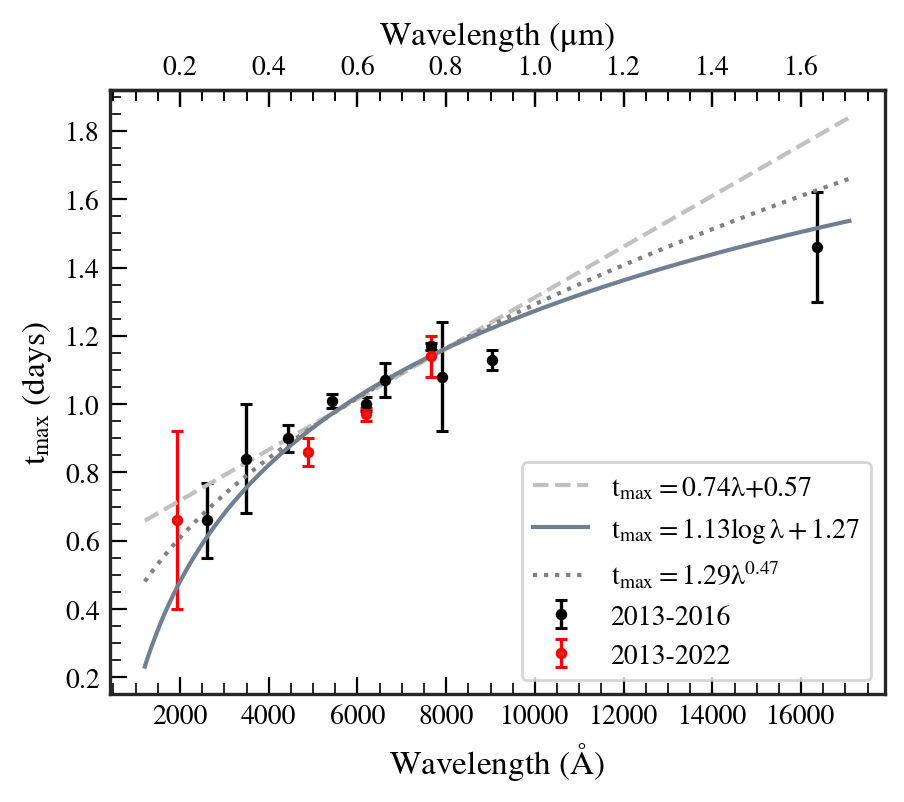
Figure 8: Plot of $\rm t_{max}$ vs wavelength. Shown in red are derived from modelling the $2013-2022$ data in $uvw2$, $g^{\prime}$, $r^{\prime}$, and $i^{\prime}$ bands. Data obtained until 2016 are shown in black. The best-fit relations between $\rm\lambda~{}(\mu m)$ and $\rm t_{max}~{}(days)$ are given in the legend. See text for details.

This phase has been modelled with a quadratic function to trace the rise to the peak and the fall just after. Limited availability of $uvw2$ data during this phase led to only partial modelling of the rise in this band. On the other hand, the optical bands have dense coverage of the rise and the peak. The $uvw2$ and $g^{\prime}$ bands show a smooth rise towards the peak and a smooth decline from the peak. In contrast, the $r^{\prime}$ and $i^{\prime}$ bands show a “cusp” just before the peak of the modelled light curve is attained.

On combining the $2013-2015$ light curves with those from $2017-2022$, we clearly see the cusp (Figure 7), at least in $r^{\prime}$ and $i^{\prime}$ bands, just before the peak is attained. The cusp-like feature is evident in the 2021 and 2022 light curves (Figure 4) as the data points are dense. The 2018 light curve also indicates the presence of the cusp, although with lesser brightness. The 2017 $V$ band and 2019 $R$ band data also hint at the cusp. Observations post-2016 indicate that the cusp is most likely present during all eruptions. The cusp was first noted by Henze et al. (2018e) in the 2016 eruption in multiple wavebands, and they argued whether the “cusp” feature could be an isolated event in 2016 and was connected to the short SSS phase and long inter-eruption period of the 2016 event. We suggest this feature is a general trend and not connected to the shorter SSS phase of 2016. However, to confirm it, we encourage very early detection and dense observations during the rise phase in all UVOIR bands of future eruptions.

The time of maxima was calculated from the quadratic model fits to the data near the peak. The peak magnitudes and the time of the peak are given in Table 4. The time lag of the peaks in different wavebands is shown in Figure 8. As expected in thermonuclear processes, the time delay increases towards longer wavelengths. Merging our uvw2 and optical bands results with those from literature, we found that a logarithmic dependence gives a better fit ($\chi^{2}=2.88$) than the linear relation (slope $=0.74\pm 0.06$ days $\rm\mu m^{-1}$; $\chi^{2}=3.34$), while the best-fit power law with an index of $0.47\pm 0.04$ ($\chi^{2}=2.94$) resulted in an intermediate fit (see Figure 8). The linear relation is close to $0.61\pm 0.11$ days $\rm\mu m^{-1}$ obtained by Darnley et al. (2016).

4.3.2 The initial steep decline

The initial decline is very fast in all the bands. The decline rates during this phase are modelled by a straight line fit from $\rm t_{max}$ to $\rm t~{}=~{}3.5$ days after the eruption. The $uvw2$ decline rate of 0.93 mag day^-1 is steeper than the $uvw1$ decline rate (0.78 mag day^-1) reported by Henze et al. (2018e). In the $2017-2022$ data, we find that the $g^{\prime}$ band decline rate (0.90 mag day^-1) is marginally higher than the $r^{\prime}$ band (0.88 mag day^-1) but when we combine it with the $2013-2015$ data, the $g^{\prime}$ band decline rate (0.90 mag day^-1) is less than the $r^{\prime}$ band (0.97 mag day^-1). Darnley et al. (2016) noted that the decline is fastest in $V$ (1.21 mag day^-1) whereas the $B$ and $r^{\prime}$ decline rates (in mag day^-1) are 0.99 and 0.97 respectively. The decline rates in this phase are used to derive the $t_{2}$ times given in Table 4.

4.3.3 The slow decline

The slow decline phase is modelled with a linear fit from day 3.5 onward. This phase consists of the plateau in the light curves which is also coincident with the SSS phase in X-rays. Combining all eruptions from 2013 gives a sufficient number of data points in all the filters for modelling except in $g^{\prime}$. The decline rate during this phase is low in all the bands (see Table 4). The $r^{\prime}$ band also show scatter during this linear decline, but these jitters are more prominent in the $uvw2$ filter. The $t_{3}$ time calculated from the straight line fits are 6.17, 10.83, and 14.15 days in $r^{\prime}i^{\prime}$ and $uvw2$, respectively. The slowing down of the decline rate can be attributed to the expanding ejecta cooling at $t\geq 4$ days from the eruption. It is also reflected in the colour evolution where after day 4, we see the system become redder (see Figure 6 and Figure 2 of Darnley et al. (2016)). Beyond day 8, in $uvw2$, we see a further decrease in the decline rate and model it with a different slope. Optical photometry is sparse after day 8, but some data points in the $i^{\prime}$ band are available, though not enough for modelling. The $i^{\prime}$ band excess ($0.2-0.4$ mags) around day 8 is most notable. This bump is traced by GP regression and is shown in blue in Figure 7.

During this phase, we see a secular trend of decreasing flux with jitters/re-brightenings on top of it. This scatter from the smooth decline in $uvw2$ has been discussed in §7.3. Towards the end of the final decline phase, when the SSS flux drops to zero at $t>18$, we see a brief period of UV re-brightening before fading away to quiescent.

5 The Super-soft phase in X-rays

5.1 X-ray light curve

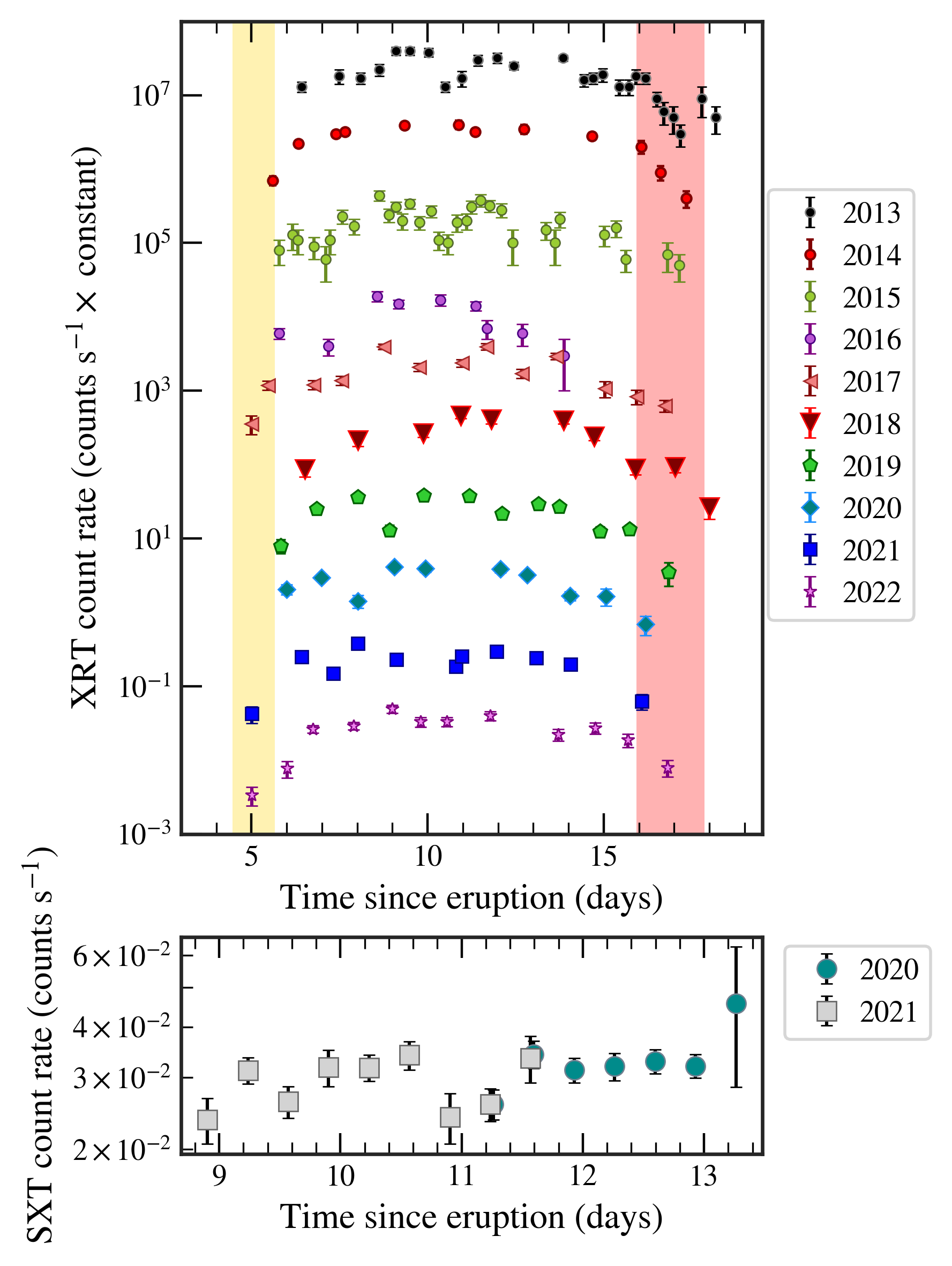
Figure 9: XRT ($2013-2022$) and SXT ($2020-2021$) light curves of M31N 2008-12a during its SSS phase. The SSS turn-on (yellow region) and turn-off (red region) times are also shown.

Figure 9 shows the light curve of supersoft X-ray emission during the $2017-2022$ eruptions. The light curves from the previous eruptions are also shown for comparison. The emergence of the SSS phase is marked by the detections at $\sim~{}8\times 10^{-3}$ counts s^-1, which increases to $(3-4)\times~{}10^{-2}$ counts s^-1 and stays around that level from 8 to 15 days after the eruption. This ‘peak’ of the SSS phase coincides with the UV light curve plateau region. The mean turn-on and turn-off time of the nova estimated from the mid-points of detections and non-detections of $2014-2022$ eruptions are $5.06\pm 0.60$ and $16.89\pm 0.96$ days, respectively from the time of the eruption. The average SSS duration of the nova is $11.83\pm 1.56$ days. Through the rise and during the SSS phase, the X-ray emission is variable, while the decline from the SSS phase is relatively smooth. Multiple “dips” are seen in the $2017-2022$ XRT light curves. One around days $6-8$, and an even more noticeable one around days $10-11$. This drop in the count rate is evident in the SXT light curves of $2020-2021$ eruptions (Figure 9). Variability in the X-ray emission during the SSS phase has also been noted in the previous eruptions by Darnley et al. (2016) and Henze et al. (2018e). The cause of this variability is not yet clear, and further high-cadence observations are required to understand its origin.

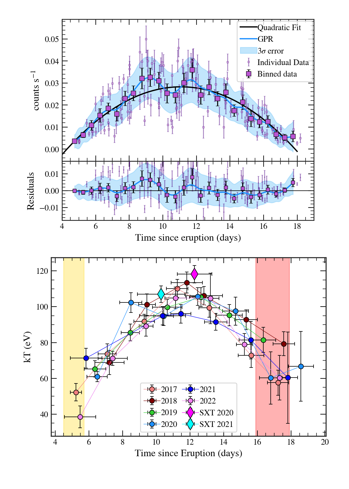
Figure 10: Top panel: Combined XRT data of the SSS phase during 2013-2022 (except 2016) eruptions. Overplotted are data points binned at 0.5 days, its quadratic fit in black, GP regression and its corresponding $3\sigma$ error region in blue. The deviations from the simple quadratic fit are shown below it. Bottom panel: Temperature evolution from XRT data during the SSS phase of $2017-2022$ eruptions. SXT data points for 2020 and 2021 are over-plotted. Mean turn-on and turn-off times are marked in yellow and red respectively.

To model the rise and decline in soft X-ray flux, we used a simple quadratic function. We included all the observations from 2013, except the peculiar 2016 eruption as its effect was seen most in the SSS phase. We plot all the individual and binned sets in Figure 10. Deviations from the naive quadratic function are evident, especially the peaks at days $9-10$ and $11-12$ and the dips at days $7-8$ and $10-11$. The prominent features between days 8 and 13 are present in the binned and unbinned data, indicating that these variabilities’ causes last for more than half a day. The drop and rise of flux between days 10-11 seem to be a general feature of the SSS phase of M31N 2008-12a. Most of the variability is seen up to day 13, whereafter, the decline is relatively smooth.

X-ray studies of M31 novae (Henze et al. 2010, 2011, 2014b) have revealed the correlation of ejecta expansion velocity and the SSS $\rm t_{on}$ time. The ejecta mass was calculated from the turn-on times and the ejecta velocities ($\rm v_{exp}$) using the relation given in Henze et al. (2014b). A $\rm t_{on}$ time of $\sim$5 days with an $\rm v_{exp}$ of $\rm\approx~{}2000~{}\pm~{}200~{}km~{}s^{-1}$ around this phase gives an ejecta mass range of $\rm 4.2~{}\times~{}10^{-8}~{}<~{}M_{ej,H}~{}/~{}M_{\odot}~{}<~{}10.2~{}\times~{}10^{-8}$. These are slightly higher than that calculated from optical spectra in §6.2 but less than the average mass accreted in a year.

5.2 X-ray spectroscopy

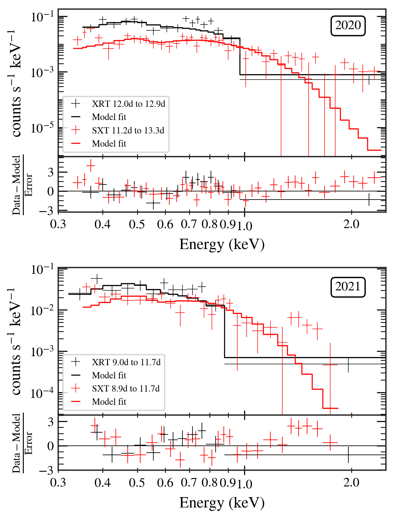
Figure 11: XRT and SXT spectra of 2020 (top panel) and 2021 (bottom panel) eruptions. XRT data nearest to the SXT observation dates have been used for better comparison. The exact observation epochs are given in the legends (in days since the eruption). Spectral fitting involved a single black body with ISM absorption models for both SXT and XRT.

The XRT data was also used to extract spectra by merging two data sets obtained on consecutive days to increase the SNR. We fixed the H column density at $\rm 1.4\times 10^{21}cm^{-2}$ (Darnley et al., 2016) but varied the blackbody temperature and normalization to attain the best-fit values. The time evolution of the SSS temperature is shown in Figure 10 for $2017-2022$ eruptions. Not only does the fluxes peak $10-14$ days after the eruption, but the temperatures also peak, suggesting a correlation between the SSS flux and temperature. In the 2020 eruption, a temperature fluctuation during the maxima can be seen. Such fluctuations have been reported before by Darnley et al. (2016). This pattern is not seen in other eruptions, possibly due to combining data sets of two consecutive days. In §5.1, it was noted that the rise to the maxima in the SSS phase shows variability, whereas the decline was smooth. The temperature evolution in Figure 10 also shows an asymmetry during the rise and decline of the SSS phase. These could be because of two different underlying causes. The increase in flux and temperature is due to the expansion and thinning of the ejecta, probing the deeper and hotter layers towards the WD surface. Whereas during the later stage, when the obscuring material is already dissipated, the decrease in flux and temperature is because of the residual nuclear burning slowing down and eventually stopping.

Spectra extracted from the merged SXT data is shown in Figure 11. Also shown are the contemporaneous XRT spectra obtained from merged snapshots of two successive days. The data has been restricted to below 2.5 keV for the SXT to avoid background contamination due to its large PSF compared to the XRT. Beyond 1 keV, the flux is too low, owing to the super-soft nature of the source. A faint hard X-ray tail (above 1.5 keV) can be seen in SXT data, but we could not be certain of its origin because of low SNR. The best-fit blackbody temperatures from SXT spectra are slightly higher than the XRT data during similar times (Figure 10). The modelled flux in the $0.3-2.0$ keV range was similar in the 2020 spectra for both instruments but differed by a factor of 2 (higher in SXT) in the 2021 spectra. As the observations are not continuous and the XRT and SXT epochs do not coincide exactly, the mismatch could be because of the rapid variability seen in flux and temperature during the SSS phase in recurrent novae.

6 Optical Spectroscopy

6.1 Spectra analysis

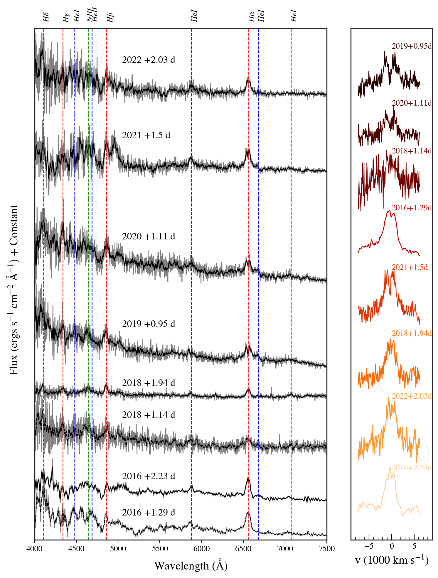
Figure 12: Left: Optical spectra obtained from HCT during 2016, and $2018-2022$ eruptions of M31N 2008-12a. Right: Time evolution of $\rm H\alpha$ morphology from top to bottom.

Table 5: Flux and FWHM velocities of identified lines in the spectra

Identification			2016 (+2.23 d)				2018 (+1.94 d)				2019 (+0.95 d)
			$\lambda$	Flux $\times 10^{-15}$	Velocity		$\lambda$	Flux $\times 10^{-15}$	Velocity		$\lambda$	Flux $\times 10^{-15}$	Velocity
			(Å)	(erg cm-2 s-1)	($\rm km~{}s^{-1}$)		(Å)	(erg cm-2 s-1)	($\rm km~{}s^{-1}$)		(Å)	(erg cm-2 s-1)	($\rm km~{}s^{-1}$)
4101	H I		$\cdots$	$\cdots$	$\cdots$		4094.52	2.37 $\pm$ 0.60	1954 $\pm$ 226		$\cdots$	$\cdots$	$\cdots$
4340	H I		4333.90	2.54 $\pm$ 0.70	1952 $\pm$ 271		4340.02	2.61 $\pm$ 0.41	3546 $\pm$ 416		4336.98	4.07 $\pm$ 0.44	2300 $\pm$ 313
4471	He I		4489.07	0.96 $\pm$ 0.30	1637 $\pm$ 258		4468.84	1.95 $\pm$ 0.47	2618 $\pm$ 409		$\cdots$	$\cdots$	$\cdots$
4640	N III		$\cdots$	$\cdots$	$\cdots$		4642.11	2.01 $\pm$ 0.42	2386 $\pm$ 279		4632.33	4.09 $\pm$ 0.36	3488 $\pm$ 222
4861	H I		4862.06	3.32 $\pm$ 0.91	2233 $\pm$ 472		4856.94	3.35 $\pm$ 0.44	2278 $\pm$ 162		4851.15	5.14 $\pm$ 0.79	2998 $\pm$ 217
5876	He I		5877.73	1.77 $\pm$ 0.37	1974 $\pm$ 217		5871.05	1.22 $\pm$ 0.45	2023 $\pm$ 336		5861.49	1.76 $\pm$ 0.25	3092 $\pm$ 292
6563	H I		6556.99	8.15 $\pm$ 0.39	2407 $\pm$ 73		6558.89	4.42 $\pm$ 0.83	2581 $\pm$ 206		6562.06	10.78 $\pm$ 1.12	5599 $\pm$ 666
6678	He I		6678.70	1.79 $\pm$ 0.50	3024 $\pm$ 477		6667.21	0.57 $\pm$ 0.12	1235 $\pm$ 195		6668.21	1.50 $\pm$ 0.36	2166 $\pm$ 423
7065	He I		7042.55	1.34 $\pm$ 0.08	2655 $\pm$ 191		7064.87	1.79 $\pm$ 0.21	3144 $\pm$ 210		7043.49	1.54 $\pm$ 0.45	2172 $\pm$ 221
Identification			2020 (+1.11 d)				2021 (+1.50 d)				2022 (+2.03 d)
			$\lambda$	Flux $\times 10^{-15}$	Velocity		$\lambda$	Flux $\times 10^{-15}$	Velocity		$\lambda$	Flux $\times 10^{-15}$	Velocity
			(Å)	(erg cm-2 s-1)	($\rm km~{}s^{-1}$)		(Å)	(erg cm-2 s-1)	($\rm km~{}s^{-1}$)		(Å)	(erg cm-2 s-1)	($\rm km~{}s^{-1}$)
4101	H I		$\cdots$	$\cdots$	$\cdots$		$\cdots$	$\cdots$	$\cdots$		$\cdots$	$\cdots$	$\cdots$
4340	H I		4335.35	56.97 $\pm$ 11.23	2244 $\pm$ 235		4331.77	0.96 $\pm$ 0.27	1506 $\pm$ 192		$\cdots$	$\cdots$	$\cdots$
4471	He I		$\cdots$	$\cdots$	$\cdots$		$\cdots$	$\cdots$	$\cdots$		$\cdots$	$\cdots$	$\cdots$
4640	N III		$\cdots$	$\cdots$	$\cdots$		$\cdots$	$\cdots$	$\cdots$		$\cdots$	$\cdots$	$\cdots$
4861	H I		4862.21	55.42 $\pm$ 10.21	3456 $\pm$ 316		4859.29	3.94 $\pm$ 0.49	2835 $\pm$ 196		4865.98	1.41 $\pm$ 0.26	1203 $\pm$ 129
5876	He I		5876.70	20.33 $\pm$ 5.39	2974 $\pm$ 387		5871.17	1.50 $\pm$ 0.13	2374 $\pm$ 139		5879.41	2.41 $\pm$ 0.18	3006 $\pm$ 168
6563	H I		6560.72	89.53 $\pm$ 8.42	5467 $\pm$ 539		6556.31	4.81 $\pm$ 0.26	3245 $\pm$ 118		6562.26	4.51 $\pm$ 0.23	2748 $\pm$ 93
6678	He I		6662.38	13.11 $\pm$ 4.42	2152 $\pm$ 362		6667.89	0.35 $\pm$ 0.05	1071 $\pm$ 88		$\cdots$	$\cdots$	$\cdots$
7065	He I		7052.56	13.66 $\pm$ 2.19	1784 $\pm$ 109		7053.60	0.43 $\pm$ 0.09	2077 $\pm$ 280		$\cdots$	$\cdots$	$\cdots$

The optical spectra with a good SNR are shown in Figure 12 with important emission features marked. Spectra taken on 2021 Nov 14.8 UT and 2022 Dec 3.73 UT were noisy and have not been used for analysis. All the spectra have been dereddened using $E(B-V)=0.10$ (Darnley et al., 2017b). The spectra were taken within the first three days of the eruption and depict a blue continuum with Hydrogen Balmer and He I (4471 Å, 5876 Å, 6678 Å) emission lines. Some epochs also show the He II (4686 Å) and the N III lines ($\sim$ 4640 Å). The FWHM of the lines and the flux values were obtained using Gaussian fitting in IRAF and are given in Table 5. The velocities calculated from the widths of the emission lines have been corrected for the instrumental response by de-convolving with the width of night skylines.

The initial velocities within 1 day of eruption are as high as 5000 km s^-1, typical of very fast novae. These observations are consistent with the previous eruption of M31N 2008-12a (Henze et al., 2018e; Darnley et al., 2016, 2015c). At around $\gtrsim 1.5$ day after the eruption, the emission line widths narrow to 3000 km s^-1. The velocity deceleration was seen to have a dependence of $\rm v_{exp}\propto t^{-0.26\pm 0.05}$. This closely resembles phase II of the shocked remnant development ($\rm v_{exp}\propto t^{-0.33}$) (Bode & Kahn, 1985). During this phase, the ejecta expands adiabatically, cooling down while sweeping the CSM.

The $\rm H\alpha$ profile morphology, as seen in Figure 12, indicates that the ejecta geometry is complicated, time-dependent, and different each year. The $\rm H\alpha$ line shows a double-peaked structure, prominent in the 2016, 2019, 2020, and 2021 spectra, taken around $\rm 0.9-1.5~{}days$ after the respective eruptions. In 2016, both profiles, with a time gap of almost 1 day, show a broad peak with a minute dip at the centre. Around day 2 after the eruption, the double-peaked profiles give way to a boxy profile as seen in Figure 12.

6.2 Estimation of physical parameters

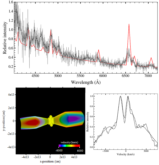
Figure 13: Top: Best-fit Cloudy modelled spectrum (solid red) overplotted on the observed spectrum (grey) and smoothed spectrum (black dotted lines) of the 2019 (+0.95 d) eruption. Bottom-left: Morphology of the ejecta of 2019 eruption obtained from Shape using H$\alpha$ velocity profile. X-axis is the line-of-sight direction, Y-axis is perpendicular to the plane of sky and line-of-sight, and Z is velocity. Bottom-right: Best-fit H$\alpha$ velocity profile (dash line) overplotted on the observed profile (solid line).

To understand the physical parameters driving the nova M31N 2008-12a, the spectral synthesis code Cloudy (v17.02; Ferland et al. 2017) was used to obtain a 1D model using the procedure mentioned in Pavana (2020). We generated a 1D model for the best SNR spectrum taken on 2019 Nov 7.6 UT. The top panel of Figure 13 shows the synthetic spectrum obtained using a two-component model. The effective temperature and luminosity of the central ionizing source were found to be $\rm 7.20\times 10^{4}~{}K$ and $\rm 10^{37}~{}erg~{}s^{-1}$ respectively. The clump component of $\rm 2.24\times 10^{10}~{}cm^{-3}$ could generate most of the emission features while a diffuse component of $\rm 1.26\times 10^{8}~{}cm^{-3}$ was used to fit the rest of the lines. The ejected mass and helium abundance from the best-fit modelled spectrum were found to be $\rm 1.3\times 10^{-8}~{}M_{\odot}$ and $\rm 3.09\pm 0.18~{}He_{\odot}$ respectively using the relations given in Pavana et al. (2019) and references therein. The ejected mass derived from X-rays and spectral modelling are similar to that reported for the 2015 eruption by Darnley et al. (2016).

It was noted that the two-component model was insufficient to generate the synthetic spectrum with a high $\chi^{2}$ value. The smoothened observed spectrum shows N II lines, which were clearly visible once a third component (diffuse) was introduced to the model. This implies that the N II and He lines are clearly originating from different regions with different physical conditions. However, since the optical spectrum of this extragalactic nova has low SNR, modelling with 3 components is beyond the scope of this work. With these uncertainties, modelling a high SNR spectrum with similar methods in the upcoming eruptions is suggested.

The H$\alpha$ emission line profile during the 2019 eruption with multiple peaks intrigued us to obtain the morpho-kinematic structure for the ejecta using Shape (Steffen et al., 2011). We carried out the morpho-kinematic analysis of the H$\alpha$ velocity profile following the procedure described in Pavana (2020). An asymmetric bipolar structure with bipolar cones and an equatorial ring (Figure 13) with a best-fit inclination angle of 79.60^∘ $\pm$ 1.45^∘ could generate the synthetic velocity profile shown in the bottom panel of Figure 13. The enhanced bipolar component extended up to 5.58 $\times$ 10¹³ cm along the ejecta axis from the centre while the bipolar conical components (opening angle of $\sim$40^∘) extended up to 6.16 $\times$ 10¹² cm. The radii of the equatorial ring and the bipolar cones were $\rm 4.12\times~{}10^{12}$ cm and $5.27\times~{}10^{12}$ cm, respectively. It should be noted that the He I (6678 Å) profile is blended with the broad H$\alpha$ profile, and interestingly, the He I line is coming from the inner regions (bipolar conical regions). The enhanced bipolar nature suggests a fast-moving polar ejecta along the ejecta axis, contributing more to the high-velocity hydrogen Balmer emission.

7 Discussion

7.1 More evidence of jets?

The cusp around maxima in the light curves has been suggested to have different origins. It could be due to shock from a secondary ejection (Kato et al., 2009), polar outflow along the line-of-sight, or ejecta-donor interaction (Darnley et al., 2018b). Observational evidence of broad-winged emission features supports the presence of a fast-moving component in the ejecta. Modelling the H$\alpha$ line profile using Shape could also generate these fast-moving polar ejecta close to the line-of-sight. Darnley et al. (2017b) proposed the presence of these jets using HST data, though they did not confirm it. In M31N 2008-12a, photometric and spectroscopic evidence combined with H$\alpha$ profile modelling presented in this work further strengthens the claim of the presence of polar jets close to the line-of-sight.

7.2 Light curve

The optical light curves from 2017 to 2022 are similar. A sharp linear decline is seen from day 1 since the maximum, followed by an approximately flat but jittery plateau and then the final decline ensues. The evolution is similar to the past eruptions and is close to the light curves of P-class recurrent novae (Strope et al., 2010).

The UV peak is observed before the optical peak in all the eruptions. The UV light curve shows a decline from peak magnitude until the onset of the plateau phase, followed by multiple jitters. The UV plateau phase is consistent with the SSS phase’s turn-on time. A flat decline follows it and ultimately ends with a brief period of brightening. The 2016 uvw2 light curve shows considerable deviation from the other eruptions.

The SSS phase turns out to be similar in all the eruptions except for the 2016 eruption, where it ended as early as $\rm\sim 16~{}days$ from the eruption. The SSS temperature is strongly correlated to the soft X-ray flux. There is a significant drop in X-ray flux during the $2017-2022$ eruptions around the same time that was noted in the previous eruptions on day 11 since the eruption. The cause of this drop in flux is yet to be explored.

During the slow decline phase, the 2016 $uvw2$ light curve (Figure 7) deviated from the general trend. We note that the F148W magnitudes during this phase in 2019-2021 are $\sim$ 1 mag fainter than the usual uvw2 magnitudes but match the outlier 2016 $uvw2$ range.

Here, we also point out that detailed $uvw2$ observations were conducted for the first time in 2016, and the light curve was found to be similar to the 2015 $uvw1$ trend (Henze et al., 2018e), although it faded earlier than that in 2015. From Figure 5, it is evident that the evolution of $uvw2$ flux in 2016 is unlike that of any eruption. Figure 7, shows that the usual trend in the 2016 $uvw2$ light curve is fainter than the average. It is very likely that the 2016 $uvw2$ evolution is connected to the distinct short-duration SSS phase of the same eruption.

7.3 UV – X-ray correlation?

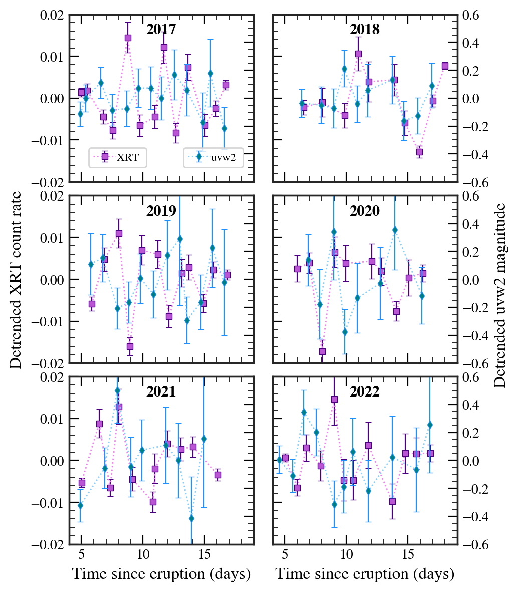
Figure 14: Detrended Swift $uvw2$ and XRT light curves for $2017-2022$ eruptions during the SSS phase.

We noticed the 2016 $uvw2$ light curve was “shorter and less luminous” compared to the $2017-2022$ $uvw2$ measurements during the SSS phase. Henze et al. (2018e) had found the same for soft X-rays and reasoned it to be due to a reduced accretion rate prior to the 2016 eruption. They could not comment on the 2016 $uvw2$ measurements because of the unavailability of the $uvw2$ light curve template at that time. This motivated us to find the connection between these two wave bands in the super-soft phase. Since both soft X-ray and UV show different trends during the super-soft phase, it was necessary to detrend them. The $uvw2$ light curves were detrended with a linear fit as it followed a linear declining trend during SSS phase, whereas the X-rays were detrended with a quadratic function as it followed a rise and a subsequent fall. The detrended light curves of each year from 2017 to 2022 are given in Figure 14. In 2017, we saw the UV and the X-ray fluxes behave inversely between days 7.5 and 13, and a Pearson correlation coefficient (hereafter $r$) value of -0.76 suggests a strong anti-correlation. In 2018, the anti-correlation lasts shorter from day 8.5 to day 11.5 but is stronger with a $r$ value of $-0.86$. 2019, on the other hand, does not show any strong correlation. In 2020 and 2022, there was a strong anti-correlation from day 9.5 to 14.5 when $r$ value was $-0.79$ and $-0.68$, respectively. The 2021 detrended light curves show mild anti-correlation ($r=-0.38$) which is stronger than 2019 but weaker than the other eruptions during the days $9-14$. This anti-correlation seen in most of the eruptions between UV and soft X-ray is strongest from day 8 to day 14 after the eruption, a time corresponding to the maxima of the SSS phase. Ness et al. (2009) noted such anti-correlation of UV and X-rays in the detrended light curves for nova V458 Vul, although in the $\rm 0.6-10~{}keV$ X-ray range, just before the start of the SSS phase, and they suggested that it would imply that both the UV and hard X-rays originate from the same region. Since the source of soft X-rays during the SSS phase is the nuclear burning on the surface of the WD, the anti-correlation during the SSS peak, in our case, would hint that the UV radiation origin is also close to the surface of the WD. The variability (jitters) could arise from the reformation of the accretion disk.

7.4 Decreasing accretion rate

In § 3, we found that the recurrence period shows an increasing trend with time. A modest increase in the recurrence period would imply that either the accretion rate or the WD mass is decreasing over the years (Hillman et al., 2016; Wang, 2018). Light curve models provided by Kato et al. (2015) suggested the WD to be as massive as $\rm 1.38~{}M_{\odot}$, accreting at a rate of $\rm 1.3~{}\times~{}10^{-7}~{}M_{\odot}~{}yr^{-1}$. Whereas Darnley et al. (2017c) modelled the quiescent phase accretion disk using HST data and showed that the rate of mass accretion could be even higher at $\rm(0.6-1.4)~{}\times~{}10^{-6}~{}M_{\odot}~{}yr^{-1}$ considering a 50% efficiency. On the other hand, the ejecta masses during each nova cycle (see § 5.1 and § 6.2) are $\rm\sim 10^{-8}M_{\odot}$. Thus, the net mass lost during each eruption is always less than the total mass gained between each eruption. As a result, the WD is growing in mass with time. The absence of Ne lines in the spectra indicates it to be a CO WD. Such WDs can reach $\rm>1.36~{}M_{\odot}$ only by accreting material. These inferences rule out the possibility of an increasing recurrence period due to decreasing WD mass. We suspect that the accretion rate has been slowly declining over the years (see Figure 2), lengthening the time taken to reach the critical conditions required for thermonuclear runaway reactions to be initiated on the surface of the WD. The following could cause a gradual decrease in the accretion rate:

1. The presence of starspots and increased activity in the secondary (Henze et al., 2018e).

2. The companion slowly running out of gas by supplying material to power the “H flashes” for millions of years (Darnley et al., 2019c).

3. Orbital dynamics can also change accretion rates, especially in violent systems like M31N 2008-12a, where nova eruptions are frequent.

4. Extent of the destruction of the accretion disk during each nova eruption decides the time taken to reform the accretion disk and resumption of accretion. Delayed accretion can also lead to a slowing down of the recurrence period.

5. A third body orbiting the M31N 2008-12a CV could perturb the binary motion, changing the accretion rate. Triple systems are known to produce exotic binaries; one such example is T Pyx (Knigge et al., 2022).

8 Summary

This paper presents the evolution of $2017-2022$ eruptions of M31N 2008-12a in different wavelengths. The main results are summarised as follows.

1. The linear decline post-maximum in the optical light curves is similar to that of the previous eruptions. The evolution of the UV light curve in the $2017-2022$ eruptions is also similar to the previous eruptions. A rapid decline since the maximum is followed by a plateau phase coincident with the SSS turn-on time. It then follows a secular decline with jitters before dimming beyond the detection limit. A UV rebrightening is also seen towards the end of the SSS phase.

2. The mean SSS turn-on time and turn-off time are 5.1 $\pm$ 0.6 days and 16.9 $\pm$ 1.0 days since the eruption respectively. The SSS phase shows X-ray variability, the most prominent being the dip $\sim$ 11 days after the eruption.

3. The UV and soft X-ray flux are anti-correlated at the peak of the SSS phase, indicating that both originate at the surface of the WD.

4. Balmer, He, and N lines dominate the optical spectra. H$\alpha$ velocities decelerate from $\sim$ 5000 km s^-1 within 1 day of eruption to $\sim$ 2000 km s^-1 at around 4 days after eruption, consistent with phase II of shock remnant development.

5. The ejecta mass derived from $\rm t_{on}$ and Cloudy modelling is of the order of $\rm 10^{-8}-10^{-7}~{}M_{\odot}$, which is less than the average mass accreted in a year, implying the WD is, potentially, increasing its mass.

6. He abundance in the ejecta was found to be very high at $\rm He/He_{\odot}=3.09$.

7. H$\alpha$ line morphology indicates an ejecta with an equatorial ring (slow-moving component) and two bipolar cones (fast-moving components) along the ejecta axis.

8. Evidence of a cusp-like feature in the light curves near the peak is seen as a general trend after the 2016 eruption in the $r^{\prime}$ and $i^{\prime}$ bands. Together with emission-line modelling, we conjecture the cusp is caused by jets present in the ejecta.

9. The recurrence period shows a weak tendency to increase with time, which is a sign of decreasing accretion rate.

10. By comparing the recurrence period with binary evolution models, the mass of the WD is constrained to be $\rm>1.36~{}M_{\odot}$. Such CO WDs near the $\rm M_{Ch}$ and growing in mass are good candidates for the single degenerate channel of Type Ia supernova explosions.

9 Acknowledgement

We are grateful to the support staff and the observers at VBO and IAO. We take this opportunity to thank the TAC for the time allocation for ToO observations. We thank the staff of IAO, Hanle and CREST, Hosakote, that made these observations possible. The facilities at IAO, CREST, and VBO are operated by the Indian Institute of Astrophysics, Bangalore. We acknowledge the use of GROWTH-India telescope data. The GROWTH-India telescope (GIT) is a 70 cm telescope with a 0.7^∘ field of view set up by the Indian Institute of Astrophysics (IIA) and the Indian Institute of Technology Bombay (IITB) with funding from the Indo-US Science and Technology Forum and the Science and Engineering Research Board, Department of Science and Technology, Government of India. It is located at the Indian Astronomical Observatory (IAO, Hanle). We acknowledge funding by the IITB alumni batch of 1994, which partially supports the operation of the telescope. Telescope technical details are available at https://sites.google.com/view/growthindia/. This work uses the SXT and UVIT data from the AstroSat mission of the Indian Space Research Organisation (ISRO). We thank the AstroSat TAC for allowing us ToO time to observe this nova from 2019-2022. We thank the SXT and UVIT payload operation centres for verifying and releasing the data via the ISSDC data archive and providing the necessary software tools. We acknowledge the use of public data from the Swift data archive. This work has also used software and/or web tools obtained from NASA’s High Energy Astrophysics Science Archive Research Center (HEASARC), a service of the Goddard Space Flight Center and the Smithsonian Astrophysical Observatory. Kulinder Pal Singh (KPS) and G.C. Anupama (GCA) thank the Indian National Science Academy for support under the INSA Senior Scientist Programme.

References

- Agnihotri & Raj (2018a) Agnihotri, V. K., & Raj, A. 2018a, The Astronomer’s Telegram, 12189, 1
- Agnihotri & Raj (2018b) —. 2018b, The Astronomer’s Telegram, 12204, 1
- Agnihotri et al. (2022) Agnihotri, V. K., Vora, K., Bisht, D., amp, & Raj, A. 2022, The Astronomer’s Telegram, 15787, 1
- Arnaud (1996) Arnaud, K. A. 1996, in Astronomical Society of the Pacific Conference Series, Vol. 101, Astronomical Data Analysis Software and Systems V, ed. G. H. Jacoby & J. Barnes, 17
- Barsukova et al. (2011) Barsukova, E., Fabrika, S., Hornoch, K., et al. 2011, The Astronomer’s Telegram, 3725, 1
- Basu et al. (2022) Basu, J., Barway, S., Anupama, G. C., & Sujith, D. S. 2022, The Astronomer’s Telegram, 15790, 1
- Bertin & Arnouts (1996) Bertin, E., & Arnouts, S. 1996, A&AS, 117, 393, doi: 10.1051/aas:1996164
- Bertin et al. (2002) Bertin, E., Mellier, Y., Radovich, M., et al. 2002, in Astronomical Society of the Pacific Conference Series, Vol. 281, Astronomical Data Analysis Software and Systems XI, ed. D. A. Bohlender, D. Durand, & T. H. Handley, 228
- Bode & Kahn (1985) Bode, M. F., & Kahn, F. D. 1985, MNRAS, 217, 205, doi: 10.1093/mnras/217.1.205
- Boyd et al. (2017) Boyd, D., Hornoch, K., Henze, M., et al. 2017, The Astronomer’s Telegram, 11116, 1
- Breeveld et al. (2011) Breeveld, A. A., Landsman, W., Holland, S. T., et al. 2011, in American Institute of Physics Conference Series, Vol. 1358, Gamma Ray Bursts 2010, ed. J. E. McEnery, J. L. Racusin, & N. Gehrels, 373–376, doi: 10.1063/1.3621807
- Burrows et al. (2005) Burrows, D. N., Hill, J. E., Nousek, J. A., et al. 2005, Space Sci. Rev., 120, 165, doi: 10.1007/s11214-005-5097-2
- Darnley (2020) Darnley, M. J. 2020, The Astronomer’s Telegram, 14138, 1
- Darnley & Healy (2022) Darnley, M. J., & Healy, M. W. 2022, The Astronomer’s Telegram, 15788, 1
- Darnley et al. (2017a) Darnley, M. J., Healy, M. W., Henze, M., & Williams, S. C. 2017a, The Astronomer’s Telegram, 11117, 1
- Darnley et al. (2018a) —. 2018a, The Astronomer’s Telegram, 11149, 1
- Darnley et al. (2019a) Darnley, M. J., Henze, M., Hachisu, I., et al. 2019a, The Astronomer’s Telegram, 13274, 1
- Darnley et al. (2019b) —. 2019b, The Astronomer’s Telegram, 13290, 1
- Darnley et al. (2018b) Darnley, M. J., Henze, M., Shafter, A. W., et al. 2018b, The Astronomer’s Telegram, 12177
- Darnley et al. (2018c) —. 2018c, The Astronomer’s Telegram, 12179, 1
- Darnley et al. (2015a) Darnley, M. J., Henze, M., Shafter, A. W., & Kato, M. 2015a, The Astronomer’s Telegram, 7964, 1
- Darnley et al. (2015b) —. 2015b, The Astronomer’s Telegram, 7965, 1
- Darnley & Pag (2021a) Darnley, M. J., & Pag, K. L. 2021a, The Astronomer’s Telegram, 15040, 1
- Darnley & Pag (2021b) —. 2021b, The Astronomer’s Telegram, 15050, 1
- Darnley & Page (2020) Darnley, M. J., & Page, K. L. 2020, The Astronomer’s Telegram, 14142, 1
- Darnley et al. (2022) Darnley, M. J., Page, K. L., & Healy, M. W. 2022, The Astronomer’s Telegram, 15798, 1
- Darnley et al. (2020a) Darnley, M. J., Page, K. L., & Henz, M. 2020a, The Astronomer’s Telegram, 14152, 1
- Darnley et al. (2020b) Darnley, M. J., Shafter, A. W., Kafka, S., Williams, S., & Henze, M. 2020b, The Astronomer’s Telegram, 14130, 1
- Darnley et al. (2014) Darnley, M. J., Williams, S. C., Bode, M. F., et al. 2014, A&A, 563, L9, doi: 10.1051/0004-6361/201423411
- Darnley et al. (2015c) Darnley, M. J., Henze, M., Steele, I. A., et al. 2015c, A&A, 580, A45, doi: 10.1051/0004-6361/201526027
- Darnley et al. (2016) Darnley, M. J., Henze, M., Bode, M. F., et al. 2016, ApJ, 833, 149, doi: 10.3847/1538-4357/833/2/149
- Darnley et al. (2017b) Darnley, M. J., Hounsell, R., Godon, P., et al. 2017b, ApJ, 847, 35, doi: 10.3847/1538-4357/aa8867
- Darnley et al. (2017c) —. 2017c, ApJ, 849, 96, doi: 10.3847/1538-4357/aa9062
- Darnley et al. (2019c) Darnley, M. J., Hounsell, R., O’Brien, T. J., et al. 2019c, Nature, 565, 460, doi: 10.1038/s41586-018-0825-4
- Darnley et al. (2019d) Darnley, M. J., Oksanen, A., Henze, M., et al. 2019d, The Astronomer’s Telegram, 13273, 1
- Engesser et al. (2018) Engesser, M. A., Socia, Q., Wysocki, P. A., Yenawine, M., & Shafter, A. W. 2018, The Astronomer’s Telegram, 12181, 1
- Erdman et al. (2022) Erdman, P., Darnley, M. J., Healy, M. W., Shafter, A. W., & Williams, S. C. 2022, The Astronomer’s Telegram, 15802, 1
- Erdman et al. (2018) Erdman, P., Kaur, A., Hartmann, D. H., et al. 2018, The Astronomer’s Telegram, 11144, 1
- Ferland et al. (2017) Ferland, G. J., Chatzikos, M., Guzmán, F., et al. 2017, Rev. Mexicana Astron. Astrofis., 53, 385, doi: 10.48550/arXiv.1705.10877
- Förster et al. (2021) Förster, F., Cabrera-Vives, G., Castillo-Navarrete, E., et al. 2021, AJ, 161, 242, doi: 10.3847/1538-3881/abe9bc
- Galloway et al. (2020) Galloway, D. K., Ackley, K., Wiersema, K., et al. 2020, The Astronomer’s Telegram, 14141, 1
- Gehrels et al. (2004) Gehrels, N., Chincarini, G., Giommi, P., et al. 2004, ApJ, 611, 1005, doi: 10.1086/422091
- Gehrz et al. (1998) Gehrz, R. D., Truran, J. W., Williams, R. E., & Starrfield, S. 1998, PASP, 110, 3, doi: 10.1086/316107
- Ginsburg et al. (2019) Ginsburg, A., Sipőcz, B. M., Brasseur, C. E., et al. 2019, AJ, 157, 98, doi: 10.3847/1538-3881/aafc33
- Hachisu et al. (1996) Hachisu, I., Kato, M., & Nomoto, K. 1996, ApJ, 470, L97, doi: 10.1086/310303
- Harris et al. (2020) Harris, C. R., Millman, K. J., van der Walt, S. J., et al. 2020, Nature, 585, 357–362, doi: 10.1038/s41586-020-2649-2
- Henze et al. (2015a) Henze, M., Darnley, M. J., Kabashima, F., et al. 2015a, A&A, 582, L8, doi: 10.1051/0004-6361/201527168
- Henze et al. (2016a) Henze, M., Darnley, M. J., Shafter, A. W., et al. 2016a, The Astronomer’s Telegram, 9853, 1
- Henze et al. (2016b) —. 2016b, The Astronomer’s Telegram, 9872, 1
- Henze et al. (2018a) —. 2018a, The Astronomer’s Telegram, 12182, 1
- Henze et al. (2018b) —. 2018b, The Astronomer’s Telegram, 11121, 1
- Henze et al. (2018c) —. 2018c, The Astronomer’s Telegram, 11130, 1
- Henze et al. (2018d) —. 2018d, The Astronomer’s Telegram, 12207, 1
- Henze et al. (2014a) Henze, M., Ness, J. U., Darnley, M. J., et al. 2014a, A&A, 563, L8, doi: 10.1051/0004-6361/201423410
- Henze et al. (2010) Henze, M., Pietsch, W., Haberl, F., et al. 2010, A&A, 523, A89, doi: 10.1051/0004-6361/201014710
- Henze et al. (2011) —. 2011, A&A, 533, A52, doi: 10.1051/0004-6361/201015887
- Henze et al. (2014b) —. 2014b, A&A, 563, A2, doi: 10.1051/0004-6361/201322426
- Henze et al. (2015b) Henze, M., Ness, J.-U., Darnley, M. J., et al. 2015b, A&A, 580, A46, doi: 10.1051/0004-6361/201526028
- Henze et al. (2015c) Henze, M., Darnley, M. J., Shafter, A. W., et al. 2015c, The Astronomer’s Telegram, 7984, 1
- Henze et al. (2018e) Henze, M., Darnley, M. J., Williams, S. C., et al. 2018e, ApJ, 857, 68, doi: 10.3847/1538-4357/aab6a6
- Hernanz & Jose (1998) Hernanz, M., & Jose, J. 1998, in Astronomical Society of the Pacific Conference Series, Vol. 137, Wild Stars in the Old West, ed. S. Howell, E. Kuulkers, & C. Woodward, 368
- Hillman et al. (2016) Hillman, Y., Prialnik, D., Kovetz, A., & Shara, M. M. 2016, ApJ, 819, 168, doi: 10.3847/0004-637X/819/2/168
- Hornoch et al. (2018) Hornoch, K., Kucakova, H., Henze, M., et al. 2018, The Astronomer’s Telegram, 11124, 1
- Hornoch et al. (2019) Hornoch, K., Kucakova, H., Wolf, M., et al. 2019, The Astronomer’s Telegram, 13279, 1
- Horst et al. (2019) Horst, J. C., Abreu, B. M., Amiri, M. I., et al. 2019, The Astronomer’s Telegram, 13281, 1
- Hunter (2007) Hunter, J. D. 2007, Computing in Science & Engineering, 9, 90, doi: 10.1109/MCSE.2007.55
- Itagaki et al. (2016) Itagaki, K., Gao, X., Darnley, M. J., et al. 2016, The Astronomer’s Telegram, 9848, 1
- Itagaki et al. (2021) Itagaki, K., Vanmunster, T., Watanabe, F., et al. 2021, The Astronomer’s Telegram, 15034, 1
- Jester et al. (2005) Jester, S., Schneider, D. P., Richards, G. T., et al. 2005, AJ, 130, 873, doi: 10.1086/432466
- K. (2016) K., I. 2016, J00452885, 4154097
- Kato & Hachisu (1994) Kato, M., & Hachisu, I. 1994, ApJ, 437, 802, doi: 10.1086/175041
- Kato et al. (2015) Kato, M., Saio, H., & Hachisu, I. 2015, ApJ, 808, 52, doi: 10.1088/0004-637X/808/1/52
- Kato et al. (2014) Kato, M., Saio, H., Hachisu, I., & Nomoto, K. 2014, ApJ, 793, 136, doi: 10.1088/0004-637X/793/2/136
- Kato et al. (2009) Kato, T., Nakajima, K., Maehara, H., & Kiyota, S. 2009, arXiv e-prints. https://arxiv.org/abs/0904.2228
- Kaur et al. (2018a) Kaur, A., Hartmann, D. H., Gonzalez, G., et al. 2018a, The Astronomer’s Telegram, 11134, 1
- Kaur et al. (2018b) Kaur, A., Hartmann, D. H., Henze, M., Shafter, A., & Darnley, M. 2018b, The Astronomer’s Telegram, 11125, 1
- Kaur et al. (2018c) Kaur, A., Hartmann, D. H., Henze, M., Shafter, A., & Darnley, M. J. 2018c, The Astronomer’s Telegram, 11126, 1
- Kaur et al. (2019) Kaur, A., Rajagopal, M., Hartmann, D. H., et al. 2019, The Astronomer’s Telegram, 13302, 1
- Kaur et al. (2018d) —. 2018d, The Astronomer’s Telegram, 12205
- Knigge et al. (2022) Knigge, C., Toonen, S., & Boekholt, T. C. N. 2022, MNRAS, 514, 1895, doi: 10.1093/mnras/stac1336
- Korotkiy & Elenin (2011) Korotkiy, S., & Elenin, L. 2011, J00452885, 4154094
- Kumar et al. (2022) Kumar, H., Bhalerao, V., Anupama, G. C., et al. 2022, AJ, 164, 90, doi: 10.3847/1538-3881/ac7bea
- McKinney et al. (2010) McKinney, W., et al. 2010, in Proceedings of the 9th Python in Science Conference, Vol. 445, Austin, TX, 51–56
- Naito et al. (2018a) Naito, H., Watanabe, F., Sano, Y., et al. 2018a, The Astronomer’s Telegram, 11133, 1
- Naito et al. (2018b) —. 2018b, The Astronomer’s Telegram, 11133, 1
- Naito et al. (2021) Naito, H., Kiyota, S., Sano, Y., et al. 2021, The Astronomer’s Telegram, 15068, 1
- Nasa High Energy Astrophysics Science Archive Research Center (2014) (Heasarc) Nasa High Energy Astrophysics Science Archive Research Center (Heasarc). 2014, HEAsoft: Unified Release of FTOOLS and XANADU, Astrophysics Source Code Library, record ascl:1408.004. http://ascl.net/1408.004
- Ness et al. (2009) Ness, J. U., Drake, J. J., Beardmore, A. P., et al. 2009, AJ, 137, 4160, doi: 10.1088/0004-6256/137/5/4160
- Nishiyama & Kabashima (2008) Nishiyama, K., & Kabashima, F. 2008, CBAT IAU, http://www.cbat.eps.harvard.edu/iau/CBAT_M31.html#2008-12a
- Nishiyama & Kabashima (2012) Nishiyama, K., & Kabashima, F. 2012, J00452884, 4154095
- Nomoto et al. (2007) Nomoto, K., Saio, H., Kato, M., & Hachisu, I. 2007, ApJ, 663, 1269, doi: 10.1086/518465
- Oksanen et al. (2019) Oksanen, A., Darnley, M. J., Shafter, A. W., et al. 2019, The Astronomer’s Telegram, 13269, 1
- Pavana (2020) Pavana, M. 2020, PhD thesis, Pondicherry University, doi: 10.5281/zenodo.8310053
- Pavana et al. (2019) Pavana, M., Anche, R. M., Anupama, G. C., Ramaprakash, A. N., & Selvakumar, G. 2019, A&A, 622, A126, doi: 10.1051/0004-6361/201833728
- Pavana et al. (2018) Pavana, M., Kiran, B. S., Sujith, D. S., & Anupama, G. C. 2018, The Astronomer’s Telegram, 12195, 1
- Pedregosa et al. (2011) Pedregosa, F., Varoquaux, G., Gramfort, A., et al. 2011, Journal of Machine Learning Research, 12, 2825
- Perez-Fournon et al. (2020) Perez-Fournon, I., Alarcon, M. R., Barrios-Perez, J., et al. 2020, The Astronomer’s Telegram, 14131, 1
- Perez-Fournon et al. (2022) Perez-Fournon, I., Poidevin, F., Aznar Menargues, G., et al. 2022, The Astronomer’s Telegram, 15786, 1
- Poole et al. (2008) Poole, T. S., Breeveld, A. A., Page, M. J., et al. 2008, MNRAS, 383, 627, doi: 10.1111/j.1365-2966.2007.12563.x
- Postma & Leahy (2017) Postma, J. E., & Leahy, D. 2017, PASP, 129, 115002, doi: 10.1088/1538-3873/aa8800
- Postma & Leahy (2021) —. 2021, Journal of Astrophysics and Astronomy, 42, 30, doi: 10.1007/s12036-020-09689-w
- Prialnik & Kovetz (1995) Prialnik, D., & Kovetz, A. 1995, ApJ, 445, 789, doi: 10.1086/175741
- Rajagopal et al. (2020) Rajagopal, M., Rutherford, T., Henson, G., et al. 2020, The Astronomer’s Telegram, 14158, 1
- Rodriguez et al. (2023) Rodriguez, E. R., Menargues, G. A., Calatayud-Borras, Y., et al. 2023, The Astronomer’s Telegram, 15902, 1
- Schaefer (2010) Schaefer, B. E. 2010, VizieR Online Data Catalog, 218
- Shafter et al. (2012) Shafter, A. W., Hornoch, K., Ciardullo, J. V. R., Darnley, M. J., & Bode, M. F. 2012, The Astronomer’s Telegram, 4503, 1
- Shafter et al. (2022) Shafter, A. W., Burris, W. A., Horst, J. C., et al. 2022, The Astronomer’s Telegram, 15797, 1
- Singh et al. (2014) Singh, K. P., Tandon, S. N., Agrawal, P. C., et al. 2014, in Society of Photo-Optical Instrumentation Engineers (SPIE) Conference Series, Vol. 9144, Space Telescopes and Instrumentation 2014: Ultraviolet to Gamma Ray, ed. T. Takahashi, J.-W. A. den Herder, & M. Bautz, 91441S, doi: 10.1117/12.2062667
- Singh et al. (2017) Singh, K. P., Stewart, G. C., Westergaard, N. J., et al. 2017, Journal of Astrophysics and Astronomy, 38, 29, doi: 10.1007/s12036-017-9448-7
- Socia et al. (2018) Socia, Q., Horst, J., Shafter, A. W., & Henze, M. 2018, The Astronomer’s Telegram, 11118, 1
- Sonith et al. (2021) Sonith, L. S., Basu, J., Anupama, G. C., et al. 2021, The Astronomer’s Telegram, 15045, 1
- Starrfield (1999) Starrfield, S. 1999, Phys. Rep., 311, 371, doi: 10.1016/S0370-1573(98)00116-1
- Steffen et al. (2011) Steffen, W., Koning, N., Wenger, S., Morisset, C., & Magnor, M. 2011, IEEE Transactions on Visualization and Computer Graphics, 17, 454, doi: 10.1109/TVCG.2010.62
- Strope et al. (2010) Strope, R. J., Schaefer, B. E., & Henden, A. A. 2010, AJ, 140, 34, doi: 10.1088/0004-6256/140/1/34
- Taguchi et al. (2021) Taguchi, K., Kawabata, M., Isogai, K., et al. 2021, The Astronomer’s Telegram, 15039, 1
- Tan & Gao (2018) Tan, H., & Gao, X. 2018, The Astronomer’s Telegram, 12200
- Tan et al. (2021) Tan, H., Zhang, M., Zhao, J., et al. 2021, The Astronomer’s Telegram, 15037, 1
- Tan et al. (2022) Tan, H., Zhao, J., Zhang, M., et al. 2022, The Astronomer’s Telegram, 15795, 1
- Tandon et al. (2020) Tandon, S. N., Postma, J., Joseph, P., et al. 2020, AJ, 159, 158, doi: 10.3847/1538-3881/ab72a3
- Tang et al. (2013) Tang, S., Cao, Y., & Kasliwal, M. M. 2013, The Astronomer’s Telegram, 5607, 1
- Tang et al. (2014) Tang, S., Bildsten, L., Wolf, W. M., et al. 2014, ApJ, 786, 61, doi: 10.1088/0004-637X/786/1/61
- Tody (1993) Tody, D. 1993, in Astronomical Society of the Pacific Conference Series, Vol. 52, Astronomical Data Analysis Software and Systems II, ed. R. J. Hanisch, R. J. V. Brissenden, & J. Barnes, 173
- Van Rossum & Drake (2009) Van Rossum, G., & Drake, F. L. 2009, Python 3 Reference Manual (Scotts Valley, CA: CreateSpace)
- Virtanen et al. (2020) Virtanen, P., Gommers, R., Oliphant, T. E., et al. 2020, Nature Methods, 17, 261, doi: 10.1038/s41592-019-0686-2
- Wagner et al. (2021) Wagner, R. M., Woodward, C. E., Starrfield, S., Rothberg, B., & Kuhn, O. 2021, The Astronomer’s Telegram, 15036, 1
- Wang (2018) Wang, B. 2018, Research in Astronomy and Astrophysics, 18, 049, doi: 10.1088/1674-4527/18/5/49
- White et al. (1995) White, N. E., Giommi, P., Heise, J., Angelini, L., & Fantasia, S. 1995, ApJ, 445, L125, doi: 10.1086/187905
- Williams et al. (2004) Williams, B. F., Garcia, M. R., Kong, A. K. H., et al. 2004, ApJ, 609, 735, doi: 10.1086/421315
- Wilms et al. (2000) Wilms, J., Allen, A., & McCray, R. 2000, ApJ, 542, 914, doi: 10.1086/317016
- Wolf et al. (2013) Wolf, W. M., Bildsten, L., Brooks, J., & Paxton, B. 2013, ApJ, 777, 136, doi: 10.1088/0004-637X/777/2/136
- Wysocki et al. (2018) Wysocki, P. A., Socia, Q., Engesser, M. A., et al. 2018, The Astronomer’s Telegram, 12190, 1