High-order adaptive multi-domain time integration scheme for microscale lithium-ion batteries simulations

Abstract

We investigate the modeling and simulation of ionic transport and charge conservation in lithium-ion batteries (LIBs) at the microscale. It is a multiphysics problem that involves a wide range of time scales. The associated computational challenges motivate the investigation of numerical techniques that can decouple the time integration of the governing equations in the liquid electrolyte and the solid phase (active materials and current collectors). First, it is shown that semi-discretization in space of the non-dimensionalized governing equations leads to a system of index-1 semi-explicit differential algebraic equations (DAEs). Then, a new generation of strategies for multi-domain integration is presented, enabling high-order adaptive coupling of both domains in time. A simple 1D LIB half-cell code is implemented as a demonstrator of the new strategy for the simulation of different modes of cell operation. The integration of the decoupled subsystems is performed with high-order accurate implicit nonlinear solvers. The accuracy of the space discretization is assessed by comparing the numerical results to the analytical solutions. Then, temporal convergence studies demonstrate the accuracy of the new multi-domain coupling approach. Finally, the accuracy and computational efficiency of the adaptive coupling strategy are discussed in the light of the conditioning of the decoupled subproblems compared to the one of the fully-coupled problem. This new approach will constitute a key ingredient for the full scale 3D LIB high-fidelity simulations based on actual electrode microstructures.

Keywords

Lithium-ion batteries, High-order time integration methods, Adaptive multi-domain integration scheme

1 Introduction

The shift in energy paradigm is evident and, as the world moves towards more renewable energy sources, the role of chemical energy storage using batteries becomes more vital. The rechargeable lithium-ion batteries (LIBs) with high energy and power densities are one of the widely used energy storage devices [47]. They are especially used in electric transportation and aerospace applications due to their portability, robustness, and reliability. In recent years, the demand has also been growing for stationary storage applications, notably in the areas of renewable energy production and grid frequency regulation. Given the established popularity of LIBs and the increase in demand, the improvement in LIB design and performance is an appealing and growing area of research. In this context, numerical simulation is an important tool, besides experimental studies, to gain insight into the functioning of LIBs. The reliability of such simulations depends on our ability to model LIBs mathematically and to devise accurate and efficient numerical methods.

The LIB operation is governed by physical phenomena at different spatial and temporal scales. The mathematical modeling of LIB yields a multiphysics and multiscale problem. From an engineering perspective, the macroscale of interest is defined by the size of a battery cell or a stack of cells. Macroscale models, such as volume-averaged [18, 10] or equivalent circuit models [31], benefit from their simplicity and are widely used in practice, e.g., for the electric and thermal control of LIBs [9, 3]. However, they suffer from severe limitations, such as loss of resolution due to volume averaging and failure to capture the effect of heterogeneities or defects in the electrode microstructure [29, 33]. Better resolution can be achieved with microscale models, accounting for the real microstructure of porous electrodes [26, 23], or with nanoscale models that can represent complex interfacial phenomena, like Solid Electrolyte Interphase (SEI) formation in graphite anodes [34, 42]. Over the last two decades, the development of such descriptions has benefited from the improvement of high-resolution imaging and high-performance computing. As a result, microscale models now offer a good compromise between complexity and accuracy at the electrode scale.

Microscale LIB models are based on a micro-continuum description of transport phenomena and electrochemistry. In these models, each point belongs to a specific material domain, such as electrolyte, active material, separator, or current collector. Within each domain, governing equations may be written for the conservation of mass, electric charge, and energy. At each material interface, specific conditions should be supplied, such as the Butler-Volmer equation modeling the charge transfer at the solid-electrolyte interface [28]. In the liquid electrolyte domain, the mathematical description of ionic transport is given by the Nernst-Planck equation for dilute solutions or the Maxwell-Stefan theory for concentrated solutions [37]. In general, the expression of charge conservation assumes solution electroneutrality, except near the electric double layer (EDL). However, in the scope of microscale models, EDL effects can be neglected as the pore size is usually much larger than the Debye length. In each active material domain, the transport of lithium is commonly represented by Fick’s law and electronic conduction by Ohm’s law. Such description relies on an effective diffusion coefficient that can be measured experimentally under representative operating conditions. It is ideally suited for active materials with solid-solution behavior, but also applicable with a lesser degree of accuracy to phase-separating materials like graphite and lithium iron phosphate (LFP).

In their standard formulation, microscale models rely on the previously mentioned assumptions that limit their domain of validity. Yet more comprehensive formulations are available, including for example thermal effects [28, 29] or mechanical deformations due to active material swelling [5, 38, 15]. Lithium plating, SEI growth, and phase changes of the active material were also considered in [21, 40, 22, 7]. The importance of including those effects depends strongly on the choice of LIB materials and the operating conditions. In a wide range of applications, however, a standard microscale formulation is sufficient to reproduce experimental charge-discharge curves within acceptable accuracy [30, 1, 48].

The numerical solution of microscale LIB models can be obtained with various simulation techniques already adopted in other fields of computational physics. In [36, 44], a discretization of the LIB microscale equations based on the finite volume method is presented. It is implemented in BESTmicro [16], a commercial LIB simulator using Cartesian meshes, as well as in the CFD-based simulation software STAR-CCM$+$^® using unstructured meshes [41]. A simulation package for the microscale study of LIBs is also available in the finite-element software COMSOL Multiphysics^® [8]. Besides commercial tools, several research simulators have been developed to model the microscale physics of LIBs based on the finite-element method [39, 43].

Simulation of LIB cells at the microscale presents multiple computational challenges. The spatial discretization of the governing equations yields a stiff system of equations, which is commonly seen in multiphysics and multiscale problems. Moreover, the Butler-Volmer current interface condition introduces a strong nonlinearity into the system. Last but not least, 3D simulation of LIBs based on real electrode microstructures requires large number of degrees of freedom (DOFs) and inversion of large ill-conditioned linear systems.

An efficient way to solve numerically stiff systems of nonlinear equations is to use stable implicit solvers [20, 6]. However, such solvers are complex to implement and require costly Newton iterations, all the more because of the ill-conditioning of the related linear systems to be solved. In [25, 24], three algorithms of time integration with domain splitting are proposed to reduce the number of Newton iterations. Convergence and stability of these algorithms are also studied for a 2D LIB model problem. In [19], another splitting approach is implemented, where lithium concentrations and electric potentials are solved independently and subsequently coupled using Picard outer-iterations. A mortar-based spatial coupling scheme allows the use of different finite-element meshes in the electrolyte and electrode phases in [13], while using a monolithic time integration approach. In [1], a domain-splitting technique in time is complemented with the block Gauß-Seidel (BGS) method and algebraic multigrid (AMG) for matrix inversion to solve the 3D LIB problem. The performance of these methods is studied in comparison with a direct linear solver. Linear solvers relying on block preconditioners corresponding to the concentration and potential fields show improved computational efficiency [14]. Overcoming the numerous challenges associated with the microscale simulation of LIBs remains an active area of research. Most of the present studies neglect the physical complexities of LIBs, such as active material phase transformations, lithium plating, mechanical effects, etc. Before adding more physics to the LIB model, there is a strong need for innovative strategies to conduct high-fidelity simulations with a high level of accuracy and robustness, but also at a reasonable computational cost.

In this work, we introduce and assess a novel multi-domain technique based on high-order adaptive coupling in time. The objective is to cope with the strong multi-scale character of the LIB model as efficiently as possible, while maintaining a coupling strategy with excellent properties of stability and accuracy. The novelty relies on the introduction of a coupling technique, which is adaptive and high-order in time. The purpose of our contribution is threefold. First, we make a precise link between a representative half-cell LIB modeling and the mathematical structure of the semi-discretized system of partial differential equations in one dimension, which includes most of the difficulties, we will have to cope with in the multi-dimensional system. We formulate the problem under the form of a system of index-1 semi-explicit differential algebraic equations (DAEs), for which accurate and stable time integrators exist. Second, we present the novel high-order and adaptive multi-domain time-coupling strategy and its analysis. Third, the numerical strategy is assessed after a series of verifications cases provided in the supplementary material. We show that the linear systems involved in the segregated domain problems are better conditioned than those of the monolithic fully-coupled approach. This indicates a strong potential of our method for 3D LIB cell high-fidelity simulations based on real electrode microstructures.

The paper is organized as follows. We introduce the 1D mathematical model for LIB half-cells in Section 2 and analyze the structure of the semi-discretized in space system of equations. We describe the numerical methods used for solving the LIB problem, including the multi-domain high-order adaptive coupling in time, in Section 3. We present and discuss our results in Section 4, which assess the strategy. Finally, relying on a study of the conditioning provided in the supplementary material, we conclude in Section 5 on the potential of the approach for realistic 3D simulations.

2 1D LIB half-cell model

In this section, we present the governing equations of the 1D LIB half-cell model along with its initial and boundary conditions. Introducing characteristic scales, we derive a non-dimensional formulation. We then apply a spatial discretization on a finite volume grid. Finally, we describe the mathematical nature of the discretized system of equations.

2.1 The microscale continuum description

The LIB operation is governed by coupled equations of mass and charge conservation in the domains of electrolyte, active material, and current collector. A schematic diagram of a 1D half-cell is shown in Figure 2.1. Here the anode consists of lithium metal, which can be simply modeled as a boundary condition on the electrolyte variables (see Equation 2.10 below). Compared to a full-cell model, the half-cell model is expected to exhibit similar numerical complexity. Indeed, the anode and cathode of the full-cell model are governed by the same equations (although with different parameters). We will now look at the governing equations and parameters in each domain as well as the boundary and initial conditions.

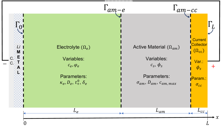
Figure 2.1: Schematic diagram of the 1D LIB half-cell model.

2.1.1 Electrolyte

The electrolyte domain $\Omega_{e}$ represents the liquid electrolyte of the LIB cell, assumed here to consist of a single lithium salt. Using the electroneutrality assumption and the concentrated solution theory, the following equations for mass and charge conservation can be derived with the proper definition of lithium-ion molar flux ${\mathbf{N}}_{e}$ and ionic current density ${\mathbf{i}}_{e}$ [35]

$$\frac{\partial{c}_{e}}{\partial t} =-\nabla\cdot{\mathbf{N}}_{e},\quad{\mathbf{N}}_{e}\left({c}_{e},{\varphi}_{e}\right)=-{D}_{e}\nabla{c}_{e}+\frac{t_{+}^{0}}{F}{\mathbf{i}}_{e},$$ (2.1)

$$0 =-\nabla\cdot{\mathbf{i}}_{e},\quad{\mathbf{i}}_{e}\left({c}_{e},{\varphi}_{e}\right)=-{\kappa}_{e}\nabla{\varphi}_{e}+\frac{2RT(1-t_{+}^{0})}{F}(1+{\delta}_{e}){\kappa}_{e}\nabla\ln{c}_{e}.$$ (2.2)

Here $F$ is Faraday’s constant, $R$ is the ideal gas constant, and $T$ is the ambient temperature. The independent variables ${c}_{e}$ and ${\varphi}_{e}$ represent lithium-ion concentration and electrochemical potential, respectively. The electrochemical potential is defined as ${\varphi}_{e}={\mu}_{e}/F+{\Phi}_{e}$, which is composed of electric potential ${\Phi}_{e}$ and chemical potential ${\mu}_{e}$ of the electrolyte. Model parameters include the transference number $t_{+}^{0}$, the electrolyte diffusivity coefficient ${D}_{e}$, the ionic conductivity ${\kappa}_{e}$, and the logarithmic derivative of the activity coefficient with respect to concentration, ${\delta}_{e}$. This coefficient appears due to the classical relation between chemical potential and ionic concentration. In this work, the concentration dependency of these parameters is neglected.

2.1.2 Electrode

The electrode (solid) domain ${\Omega}_{s}$ consists of the active material domain ${\Omega}_{am}$ and the current collector domain ${\Omega}_{cc}$. The governing equations for lithium transport and electric charge conservation in ${\Omega}_{am}$, as well as lithium molar flux ${\mathbf{N}}_{s}$ and electric current density ${\mathbf{i}}_{s}$, are given by

$$\frac{\partial{c}_{s}}{\partial t} =-\nabla\cdot{\mathbf{N}}_{s},\quad{\mathbf{N}}_{s}\left({c}_{s}\right)=-{D}_{am}\nabla{{c}_{s}},$$ (2.3)

$$0 =-\nabla\cdot{\mathbf{i}}_{s},\quad{\mathbf{i}}_{s}\left({\phi}_{s}\right)=-{\sigma}_{am}\nabla{\phi}_{s}.$$ (2.4)

Here independent variables are lithium concentration ${c}_{s}$ and electric potential ${\phi}_{s}$. Model parameters include the active material diffusivity coefficient ${D}_{am}$ and electric conductivity ${\sigma}_{am}$, which are assumed to be constant.

The current collector does not allow lithium intercalation or de-intercalation. Therefore, it is simply described by the charge conservation of Equation 2.4, where the electric current density ${\mathbf{i}}_{s}$ is now given by

$${\mathbf{i}}_{s}\left({\phi}_{s}\right)=-{\sigma}_{cc}\nabla{\phi}_{s}.$$ (2.5)

Here ${\sigma}_{cc}$ is the electric conductivity of the current collector. Typically ${\sigma}_{cc}\gg{\sigma}_{am}$, i.e., the current collector is a much better electronic conductor than the active material.

2.1.3 Boundary and initial conditions

In Figure 2.1, external boundaries of the cell located at $x=0$ and $x=L$ are denoted as $\Gamma_{0}$ and $\Gamma_{L}$, respectively. Further, internal boundaries exist at interfaces between material domains, between electrolyte and active material ($\Gamma_{am-e}$), and between active material and current collector ($\Gamma_{am-cc}$). The boundary conditions at these interfaces are often referred to as interface conditions.

The lithium exchange (intercalation/de-intercalation) between electrolyte and electrodes takes place at $\Gamma_{0}$ and $\Gamma_{am-e}$ via the redox reaction $\rm{Li}^{+}+\rm{e}^{-}\rightleftharpoons\rm{Li}$. This process is modeled as an effective exchange current density at the interface which is described by the Butler-Volmer model [4]. It is given by

$$i_{BV} =i_{0}\left(e^{\frac{\alpha F}{RT}\eta}-e^{-\frac{(1-\alpha)F}{RT}\eta}\right),$$ (2.6)

where $i_{0}$ denotes the equilibrium exchange current density, $\alpha$ is the anodic strength coefficient and $\eta$ is the electrode overpotential defined by

$$\eta ={\phi}_{s}-{\varphi}_{e}-U_{0}({c}_{s}).$$ (2.7)

Here $U_{0}$ is the open-circuit potential of the electrode, which is a function of lithium concentration in active material. At $\Gamma_{am-e}$, $i_{0}=Fk_{0}\sqrt{{c}_{e}{c}_{s}\left(c_{s,\rm{max}}-{c}_{s}\right)}$, where $k_{0}$ is the reaction rate constant and $c_{s,\rm{max}}$ is the maximum lithium concentration in active material. At $\Gamma_{0}$, the lithium metal anode leads to a simplified interface condition, with ${\phi}_{s}=$ 0 and $U_{0}=$ 0, hence $\eta=-{\varphi}_{e}$. Moreover, the equilibrium exchange current density of lithium metal is assumed to be constant. It is denoted as $i_{0,\rm{Li}}$.

In our study, we consider symmetric interface redox reactions, i.e. $\alpha=$ 0.5. The resulting current densities at the anode ($\Gamma_{0}$) and cathode ($\Gamma_{am-e}$) interfaces are

$$i_{BV}^{(A)} =2i_{0,\rm{Li}}\sinh\left(-\frac{F}{2RT}{\varphi}_{e}\right),$$ (2.8)

$$i_{BV}^{(C)} =2Fk_{0}\sqrt{{c}_{e}{c}_{s}\left(c_{s,\rm{max}}-{c}_{s}\right)}\sinh\left(\frac{F}{2RT}\left({\phi}_{s}-{\varphi}_{e}-U_{0}({c}_{s})\right)\right),$$ (2.9)

where superscripts $(A)$ and $(C)$ denote the anode and cathode, respectively. Therefore, at $\Gamma_{0}$

$${N}_{e}\left({c}_{e},{\varphi}_{e}\right)|_{\Gamma_{0}} =\frac{i_{BV}^{(A)}}{F},\quad{i}_{e}\left({c}_{e},{\varphi}_{e}\right)|_{\Gamma_{0}}=i_{BV}^{(A)},$$ (2.10)

while at $\Gamma_{am-e}$

$${N}_{e}\left({c}_{e},{\varphi}_{e}\right)|_{\Gamma_{am-e}} =-\frac{i_{BV}^{(C)}}{F},\quad{i}_{e}\left({c}_{e},{\varphi}_{e}\right)|_{\Gamma_{am-e}}=-i_{BV}^{(C)},$$ (2.11)

$${N}_{s}\left({c}_{s}\right)|_{\Gamma_{am-e}} =-\frac{i_{BV}^{(C)}}{F},\quad{i}_{s}\left({\phi}_{s}\right)|_{\Gamma_{am-e}}=-i_{BV}^{(C)}.$$ (2.12)

Note that the fluxes in Equations 2.10 to 2.12 are scalars resulting from their dot products with 1D normal vectors.

At $\Gamma_{am-cc}$, lithium flux is not allowed, it is also assumed that electric potential and current density are continuous

$${N}_{s}\left({c}_{s}\right)|_{\Gamma_{am-cc}} =0,\quad{\phi}_{s}|_{\Gamma_{am-cc}^{(-)}}={\phi}_{s}|_{\Gamma_{am-cc}^{(+)}},\quad{i}_{s}|_{\Gamma_{am-cc}^{(-)}}={i}_{s}|_{\Gamma_{am-cc}^{(+)}},$$ (2.13)

where $(-)$ and $(+)$ signs represent the left and right neighborhoods of the interface, respectively. The above conditions mean that any contact resistance or capacitance effect between active material and current collector is neglected.

The external boundary condition at $\Gamma_{L}$ is defined by the mode of operation of the LIB cell. A constant current (galvanostatic or CC) charge$/$discharge condition imposes a constant current density at $\Gamma_{L}$. It is usually defined as the product of a reference current $i_{1C}$ (“1C” rate) by a C-rate factor $\xi$. The definition of $i_{1C}$ is based on the battery charge capacity, i.e., it is the current required for a full charge of the battery in one hour, starting from a fully discharged state. Hence, the imposed current density in CC mode is

$${i}_{s}\left({\phi}_{s}\right)|_{\Gamma_{L}} =-\xi i_{1C}.$$ (2.14)

The negative sign comes from the sign convention for electric current. Note that a positive $\xi$ indicates charging while a negative value is for discharging. Further, a constant voltage (potentiostatic or CV) mode of operation means a fixed potential $\phi_{s,\rm{ext}}$ is imposed at $\Gamma_{L}$, i.e.

$${\phi}_{s}|_{\Gamma_{L}} =\phi_{s,\rm{ext}}.$$ (2.15)

In some cases, the imposed external potential can be a function of time. Such a situation will be considered in our numerical example of Sub-Section 4.2.

Finally, the mathematical model of LIB half-cells is closed by introducing the initial conditions. Hence, we have

$${c}_{e}(x,0) =c_{e,\rm{I}},\quad{c}_{s}(x,0)=c_{s,\rm{I}},$$ (2.16)

with $c_{e,\rm{I}}$ is the initial electrolyte concentration, and $c_{s,\rm{I}}$ the initial lithium concentration in active material.

2.2 Non-dimensionalization

In the following, all characteristic scales of the problem are denoted by a star (^⋆) superscript. First, we define ${L}^{\star}=L$ as a characteristic length scale. As a potential scale, we use the ambient thermal voltage ${\Phi}^{\star}=RT/F$ in both the electrolyte and solid domains. The lithium-ion concentration in the electrolyte domain is scaled by its initial value, i.e., ${c}^{\star}_{e}=c_{e,\rm{I}}$, while the scale for lithium concentration in active material is chosen as ${c}^{\star}_{s}=c_{s,\rm{max}}$. As a common timescale for the electrolyte and solid domains, we use the electrolyte diffusion timescale, hence ${T}^{\star}=({L}^{\star})^{2}/D_{e}$. These scales are summarized in Table 5.2, which also provides definitions for the flux scales ${N}^{\star}_{e}$, ${i}^{\star}_{e}$, ${N}^{\star}_{s}$, and ${i}^{\star}_{s}$.

Using the characteristic scales defined above, we now rewrite the governing equations in terms of dimensionless variables, denoted by a tilde ($\tilde{\ }$) superscript. Therefore, in the electrolyte domain

$$\partial_{\tilde{t}}\tilde{c}_{e} =-\partial_{\tilde{x}}\tilde{N}_{e},\quad\tilde{N}_{e}\left(\tilde{c}_{e},\tilde{\varphi}_{e}\right)=-\partial_{\tilde{x}}\tilde{c}_{e}+\frac{{i}^{\star}_{e}}{{N}^{\star}_{e}}\frac{t_{+}^{0}}{F}\tilde{i}_{e},$$ (2.17)

$$0 =-\partial_{\tilde{x}}\tilde{i}_{e},\quad\tilde{i}_{e}\left(\tilde{c}_{e},\tilde{\varphi}_{e}\right)=-\partial_{\tilde{x}}\tilde{\varphi}_{e}+\frac{\kappa_{D}}{\tilde{c}_{e}}\partial_{\tilde{x}}\tilde{c}_{e}.$$ (2.18)

Here $\kappa_{D}=2(1-t_{+}^{0})(1+\delta_{e})$ is a dimensionless parameter characterizing the diffusive contribution to ionic current. The other dimensionless quantity $({i}^{\star}_{e}t_{+}^{0})/({N}^{\star}_{e}F)$ represents the ratio of electric migration flux to diffusion flux. It is usually referred to as the electric Péclet number [2]. Similarly, in the solid domain, if we note $\varepsilon_{D}=D_{am}/D_{e}$ and $\varepsilon_{\sigma}=\sigma_{am}/\sigma_{cc}$, we have

$$\partial_{\tilde{t}}\tilde{c}_{s} =-\varepsilon_{D}\partial_{\tilde{x}}\tilde{N}_{s},\quad\tilde{N}_{s}\left(\tilde{c}_{s}\right)=\begin{cases}-\partial_{\tilde{x}}\tilde{c}_{s},&\quad\tilde{x}\in\tilde{\Omega}_{am},\\ \quad 0,&\quad\tilde{x}\in\tilde{\Omega}_{cc},\end{cases}$$ (2.19)

$$0 =-\partial_{\tilde{x}}\tilde{i}_{s},\quad\tilde{i}_{s}(\tilde{\phi}_{s})=\begin{cases}-\partial_{\tilde{x}}\tilde{\phi}_{s},&\quad\tilde{x}\in\tilde{\Omega}_{am},\\ -\frac{1}{\varepsilon_{\sigma}}\partial_{\tilde{x}}\tilde{\phi}_{s},&\quad\tilde{x}\in\tilde{\Omega}_{cc}.\end{cases}$$ (2.20)

We first define a unit scale for the Butler-Volmer current density: ${i}^{\star}_{BV}=\mathrm{1\ A/m^{2}}$. Hence, the boundary conditions at $\tilde{\Gamma}_{0}$ become $\tilde{N}_{e}=\tilde{i}_{BV}^{(A)}/F{N}^{\star}_{e}$ and $\tilde{i}_{e}=\tilde{i}_{BV}^{(A)}/{i}^{\star}_{e}$. Similarly, at $\tilde{\Gamma}_{am-e}$ the dimensionless interface conditions are $\tilde{N}_{e}=-\tilde{i}_{BV}^{(C)}/F{N}^{\star}_{e}$, $\tilde{i}_{e}=-\tilde{i}_{BV}^{(C)}/{i}^{\star}_{e}$, $\tilde{N}_{s}=-\tilde{i}_{BV}^{(C)}/F{N}^{\star}_{s}$, and $\tilde{i}_{s}=-\tilde{i}_{BV}^{(C)}/{i}^{\star}_{s}$. Further, $\tilde{N}_{s}=0$ at $\tilde{\Gamma}_{am-cc}$. The current density or the potential at $\tilde{\Gamma}_{L}$, depending on the LIB operating mode, is non-dimensionalized using the flux scale ${i}^{\star}_{s}$ or the potential scale ${\Phi}^{\star}$, respectively. Finally, the initial conditions become $\tilde{c}_{e}(\tilde{x},0)=$ 1 and $\tilde{c}_{s}(\tilde{x},0)=c_{s,\rm{I}}/{c}^{\star}_{s}$.

The non-dimensionalization of the governing equations shows that the time derivatives of concentrations in electrolyte and active material differ in magnitude by a factor $\varepsilon_{D}$ (see Equation 2.19). Using typical values of $D_{am}$ and $D_{e}$, we infer that $\varepsilon_{D}\in[\mathrm{10^{-5},10^{-3}}]$. It should be noted that the coexistence of two timescales in the LIB microscale model contributes to the ill-conditioning of the problem. Hence, it motivates us to explore multi-domain techniques for time integration, where improved conditioning is expected for the subproblems in each domain due to decoupling. For simplicity, we henceforth omit the “ $\widetilde{\cdot}$ ” notation for the non-dimensional variables.

2.3 Semi-discretization in space

The finite volume method is well-suited for problems involving conservation laws such as heat and mass transfer [12]. In this work, the LIB half-cell model was derived from mass and charge conservation laws in each domain, with flux-based interface conditions. Thus, we perform the spatial discretization of the non-dimensional governing equations on a 1D finite volume grid, as illustrated in Figure 2.2. The discrete values of concentration and potential variables are located at cell centers, whereas molar fluxes and current densities are defined at cell faces. The former are denoted by subscript $i$ and the latter by subscript $i+1/2$, where $i$ is the index of the $i$-th cell. To approximate the spatial derivatives of concentration and potential, we use the second-order accurate central differencing scheme.

The discretized domains of electrolyte, active material, and current collector have ${\mathcal{N}}_{e}$, ${\mathcal{N}}_{am}$, and ${\mathcal{N}}_{cc}$ finite volume cells, respectively. Hence the number of cells in ${\Omega}_{s}$ is ${\mathcal{N}}_{s}={\mathcal{N}}_{am}+{\mathcal{N}}_{cc}$, and the total number of cells $\mathcal{N}={\mathcal{N}}_{e}+{\mathcal{N}}_{s}$. Within a given material domain $\Omega_{\alpha}$ ($\alpha=e,am,cc$), we employ a constant cell width $\Delta x_{\alpha}=L_{\alpha}/\mathcal{N}_{\alpha}$ where $L_{\alpha}$ denotes the domain length. This ensures that interfaces between domains coincide with particular faces of the finite volume grid. In the following, we assume for simplicity but without loss of generality that the domain lengths allow to define a uniform grid size $\Delta x=\Delta x_{e}=\Delta x_{am}=\Delta x_{cc}$.

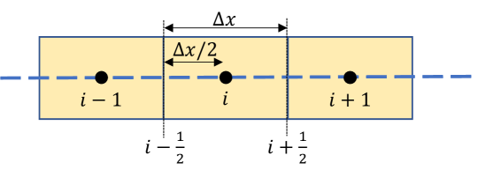
Figure 2.2: Schematic view of a 1D finite volume grid.

The system of equations obtained after spatial discretization in the electrolyte domain is given by

$$d_{t}{c}_{e,\rm{i}}={F}_{e,\rm{i}},\quad 0={G}_{e,\rm{i}},\$$ (2.21)

where, for $\text{i}=\mathrm{1,2,\ldots,{\mathcal{N}}_{e}}$, we have

$${F}_{e,\rm{i}} =-\frac{1}{\Delta x}\left({N}_{e,\rm{i+\frac{1}{2}}}-{N}_{e,\rm{i-\frac{1}{2}}}\right),\quad{G}_{e,\rm{i}}=-\frac{1}{\Delta x}\left({i}_{e,\rm{i+\frac{1}{2}}}-{i}_{e,\rm{i-\frac{1}{2}}}\right).$$ (2.22)

Here, we obtain ${N}_{e,\rm{i+\frac{1}{2}}}$ and ${i}_{e,\rm{i+\frac{1}{2}}}$ from spatial discretization of the fluxes defined in Equations 2.17 and 2.18, respectively. Similarly, in the solid domain, we have

$$d_{t}{c}_{s,\rm{j}}={F}_{s,\rm{j}},\quad\quad 0={G}_{s,\rm{j}},$$ (2.23)

where, for $\text{j}=\mathrm{1,2,\ldots,{\mathcal{N}}_{s}}$, we have

$${F}_{s,\rm{j}}= -\frac{\varepsilon_{D}}{\Delta x}\left({N}_{s,\rm{j+\frac{1}{2}}}-{N}_{s,\rm{j-\frac{1}{2}}}\right),\quad{G}_{s,\rm{j}}=-\frac{1}{\Delta x}\left({i}_{s,\rm{j+\frac{1}{2}}}-{i}_{s,\rm{j-\frac{1}{2}}}\right).$$ (2.24)

The numerical fluxes ${N}_{s,\rm{j+\frac{1}{2}}}$ and ${i}_{s,\rm{j+\frac{1}{2}}}$ are the discrete versions of Equations 2.19 and 2.20.

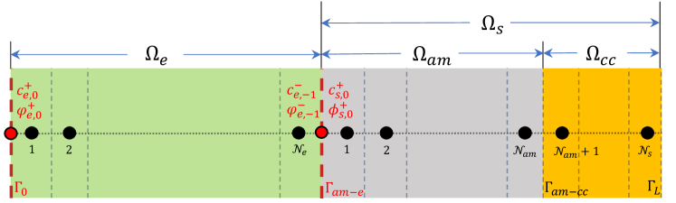
Figure 2.3: Auxiliary variables introduced at the interfaces $\Gamma_{0}$ and $\Gamma_{am-e}$ for evaluation of the Butler-Volmer current density.

In the discretized domain, molar fluxes and current densities on cell faces are defined using cell-centered variables. However, special treatment is needed at interfaces between domains and at the outer boundaries of the cell. The interface conditions at $\Gamma_{0}$ (given in Equation 2.10) and $\Gamma_{am-e}$ (given in Equations 2.11 to 2.12) require the Butler-Volmer current densities which are functions of concentrations and potentials. These variables, however, are stored at the cell centers and need to be evaluated at the interfaces $\Gamma_{0}$ and $\Gamma_{am-e}$. A simple way is to extrapolate the adjacent cell-centred variables to the interfaces. However, this method leads to inaccuracies, especially at higher current rates [48]. In this paper, we resolve this problem by employing another approach proposed in [48] involving extra variables at the interfaces. Thus, we introduce the auxiliary variables, i.e., ${c}_{e,0}^{+}$ and ${\varphi}_{e,0}^{+}$ at $\Gamma_{0}$ and ${c}_{e,-1}^{-}$, ${\varphi}_{e,-1}^{-}$, ${c}_{s,0}^{+}$ and ${\phi}_{s,0}^{+}$ at $\Gamma_{am-e}$ (see Figure 2.3). The system of discretized equations is then augmented with an auxiliary system of equations derived from the interface conditions at $\Gamma_{0}$ and $\Gamma_{am-e}$. This auxiliary system is given by the following relationships between the Butler-Volmer current density and the gradients of concentrations and potentials

$$G_{e,\rm{c}}^{(A)} :=\frac{c_{e,1}-{c}_{e,0}^{+}}{\Delta x/2}+\zeta_{e,\rm{c}}\,i_{BV}^{(A)}({c}_{e,0}^{+},{\varphi}_{e,0}^{+})=0,$$ (2.25)

$$G_{e,\rm{\phi}}^{(A)} :=\frac{\varphi_{e,1}-{\varphi}_{e,0}^{+}}{\Delta x/2}+\zeta_{e,\rm{\phi}}({c}_{e,0}^{+})\,i_{BV}^{(A)}({c}_{e,0}^{+},{\varphi}_{e,0}^{+})=0,$$ (2.26)

$$G_{e,\rm{c}}^{(C)} :=\frac{{c}_{e,-1}^{-}-c_{e,{\mathcal{N}}_{e}}}{\Delta x/2}-\zeta_{e,\rm{c}}\,i_{BV}^{(C)}({c}_{e,-1}^{-},{\varphi}_{e,-1}^{-},{c}_{s,0}^{+},{\phi}_{s,0}^{+})=0,$$ (2.27)

$$G_{e,\rm{\phi}}^{(C)} :=\frac{{\varphi}_{e,-1}^{-}-\varphi_{e,{\mathcal{N}}_{e}}}{\Delta x/2}-\zeta_{e,\rm{\phi}}({c}_{e,-1}^{-})\,i_{BV}^{(C)}({c}_{e,-1}^{-},{\varphi}_{e,-1}^{-},{c}_{s,0}^{+},{\phi}_{s,0}^{+})=0,$$ (2.28)

$$G_{s,\rm{c}}^{(C)} :=\frac{c_{s,1}-{c}_{s,0}^{+}}{\Delta x/2}-\zeta_{s,\rm{c}}\,i_{BV}^{(C)}({c}_{e,-1}^{-},{\phi}_{e,-1}^{-},{c}_{s,0}^{+},{\phi}_{s,0}^{+})=0,$$ (2.29)

$$G_{s,\rm{\phi}}^{(C)} :=\frac{\phi_{s,1}-{\phi}_{s,0}^{+}}{\Delta x/2}-\zeta_{s,\rm{\phi}}\,i_{BV}^{(C)}({c}_{e,-1}^{-},{\varphi}_{e,-1}^{-},{c}_{s,0}^{+},{\phi}_{s,0}^{+})=0.$$ (2.30)

The $\zeta$’s in Equations 2.25 to 2.30 are parameters defined below

$$\zeta_{e,\rm{c}} =\frac{1-t_{+}^{0}}{F{N}^{\star}_{e}},\quad\zeta_{e,\rm{\phi}}({c}_{e})=\frac{1}{{i}^{\star}_{e}}+\frac{\kappa_{D}}{F{N}^{\star}_{e}}\frac{1-t_{+}^{0}}{{c}_{e}},$$ (2.31)

$$\zeta_{s,\rm{c}} =\frac{1}{F{N}^{\star}_{s}},\quad\zeta_{s,\rm{\phi}}=\frac{1}{{i}^{\star}_{s}}.$$ (2.32)

Moreover, the semi-discretized system defined above has only time derivatives of concentrations, while they are absent for the potentials and the auxiliary variables. In fact, we can split these variables into differential ($W$) and algebraic ($Z$) variables

$$W =\{{c}_{e,\rm{1}},\ldots,{c}_{e,\rm{{\mathcal{N}}_{e}}},{c}_{s,\rm{1}},\ldots,{c}_{s,\rm{{\mathcal{N}}_{s}}}\},$$ (2.33)

$$Z =\{{\varphi}_{e,\rm{1}},\ldots,{\varphi}_{e,\rm{{\mathcal{N}}_{e}}},{\phi}_{s,\rm{1}},\ldots,{\phi}_{s,\rm{{\mathcal{N}}_{s}}},{c}_{e,0}^{+},{\varphi}_{e,0}^{+},{c}_{e,-1}^{-},{\varphi}_{e,-1}^{-},{c}_{s,0}^{+},{\phi}_{s,0}^{+}\}.$$ (2.34)

Consequently, we obtain a system of Differential-Algebraic Equations (DAEs)

$$\dot{W} =F(W,Z),\quad F:\mathbb{R}^{\mathcal{N}}\times\mathbb{R}^{\mathcal{N}+6}\mapsto\mathbb{R}^{\mathcal{N}},$$ (2.35)

$$0 =G(W,Z),\quad G:\mathbb{R}^{\mathcal{N}}\times\mathbb{R}^{\mathcal{N}+6}\mapsto\mathbb{R}^{\mathcal{N}+6},$$ (2.36)

where

$$F =\{{F}_{e,\rm{1}},\ldots,{F}_{e,\rm{{\mathcal{N}}_{e}}},{F}_{s,\rm{1}},\ldots,{F}_{s,\rm{{\mathcal{N}}_{s}}}\},$$ (2.37)

$$G =\{{G}_{e,\rm{1}},\ldots,{G}_{e,\rm{{\mathcal{N}}_{e}}},{G}_{s,\rm{1}},\ldots,{G}_{s,\rm{{\mathcal{N}}_{s}}},G_{e,\rm{c}}^{(A)},G_{e,\rm{\phi}}^{(A)},G_{e,\rm{c}}^{(C)},G_{e,\rm{\phi}}^{(C)},G_{s,\rm{c}}^{(C)},G_{s,\rm{\phi}}^{(C)}\}.$$ (2.38)

The equations corresponding to $W$ and $Z$ lead to the differential equations Equation 2.35 and the algebraic constraints Equation 2.36, respectively. Further, the algebraic constraints in Equation 2.36 are of two types, a discretized elliptic system of equations for the potentials ${\varphi}_{e,\rm{i}}$ and ${\phi}_{s,\rm{j}}$, and a discretized system of nonlinear Robin boundary conditions for the six auxiliary variables. Moreover, this system of DAEs is in semi-explicit or Hessenberg form. Such systems can also be found in other engineering problems, e.g. low-Mach heterogeneous combustion problems [17]. In addition, comprehensive numerical investigations show that the system of DAEs corresponding to the LIB problem is of index-1. Thus, the time integration of the semi-discretized LIB problem is effectively the integration of a system of index-1, semi-explicit DAEs. Accurate and robust integration of such problems requires specific numerical methods, which are the object of the next section.

3 Numerical schemes

In this section, we present various numerical strategies we have used to integrate the stiff system of DAEs. First, we introduce a family of implicit methods suitable for solving DAEs. Then, a multi-domain strategy for the LIB model is presented with explicit and implicit coupling strategies. Finally, an error estimate is formulated to characterize the optimal coupling frequency.

3.1 Implicit Runge-Kutta methods for DAEs

Since the 1980s, a number of integration schemes have been designed for DAE problems. Among others, backward differentiation formulae and stiffly-accurate Runge-Kutta (RK) methods have shown their efficiency and robustness [20, 6]. In our case, the stiffness induced by the fine discretization of diffusion processes and the multiscale physics invites us to contemplate L-stable methods. Based on this requirement, we can select suitable schemes available in the literature. In the present 1D study, we can afford to use the well-known Radau5 method [20], a 3-stage fully-implicit scheme, which is fifth-order accurate for index-1 DAEs and is L-stable, having proven especially successful in the integration of stiff ODEs and DAEs. However, for the larger systems expected in the full-scale 3D LIB simulations, this method can become too costly. In that case, other schemes such as the ESDIRK methods [27] can be used. They too exhibit good properties to solve DAEs, while maintaining a lower computational cost [17].

These advanced methods are in principle high-order generalizations of the implicit Euler method. This first-order method is also L-stable and copes well with the index-1 DAEs. Taking advantage of its simplicity, we take it as an illustrative example. Let us assume that the time domain $[0,\ t_{\rm{end}}]$ is divided into $N$ timesteps of equal length $\Delta t=t_{\rm{end}}/N$. Thus the discrete time values are given by $t_{n+1}=t_{n}+\Delta t$ for $n=\mathrm{0,\ 1,\ \ldots,\ \mathit{N}-1}$, where $t_{0}=0$ and $t_{N}=t_{\rm{end}}$. Applying the first-order discretization in time for the differential variables $W$, the DAEs become a system of nonlinear equations of residual function $R:\mathbb{R}^{\mathcal{N}}\times\mathbb{R}^{\mathcal{N}+6}\mapsto\mathbb{R}^{2\mathcal{N}+6}$, defined as

$$R(W^{n+1},Z^{n+1}) =\begin{bmatrix}W^{n+1}-W^{n}-\Delta t\>F(W^{n+1},Z^{n+1})\\ 0-\Delta t\>G(W^{n+1},Z^{n+1})\end{bmatrix}.$$ (3.1)

Here, the superscript $n$ represents the variables at time $t_{n}$. The nonlinear problem $R(W^{n+1},Z^{n+1})=0$ can be solved by the Newton-Raphson method, using the solution of the previous timestep (i.e., $W^{n}$ and $Z^{n}$) as initial guess. Each Newton iteration requires the solution of a linear system, which can be obtained either by direct or iterative solvers. Direct solvers are a good choice for 1D and 2D problems, since the bandwidth of the matrices to be inverted remains small. This is not the case in 3D anymore, hence iterative solvers must be considered. The performance of such solvers is however strongly deteriorated by the ill-conditioning of the matrices obtained, which is partly due to the large number of unknowns in our mixed elliptic-parabolic framework, but also to the multiphysics and multiscale nature of the problem. It is therefore crucial to use efficient preconditioners (e.g., see [1, 14]) to enable the use of iterative solvers. This topic is beyond the scope of this work and will be treated in a subsequent work devoted to the solution of the full 3D LIB model based on the technique presented in the present paper.

We now focus on the design of multi-domain techniques at the nonlinear solution level, as an alternative to costly monolithic schemes where the DAEs are integrated simultaneously over the entire computational domain with a single timestep. Note that such a technique is expected to have a strong impact on the properties of the linearized residual system (formulated among multiple domains) and related linear system solves since it yields an especially improved condition number for the subproblems that plays a crucial role in the convergence rate of iterative solvers. This statement is investigated in the supplementary material for the sake of completeness.

3.2 Multi-domain time integration method

As discussed in Section 1, the LIB model is a multiphysics as well as multiscale problem, where the Butler-Volmer current density at solid-electrolyte interfaces introduces strong nonlinearity. Mathematically, this results in a system of DAEs, which are stiff and costly to solve. The inefficiency and cost of the solution is strongly impacted by the size of the fully coupled problem. Hence, we propose to use a multi-domain technique splitting the monolithic problem into smaller decoupled subproblems. Such methods have been implemented and studied for the fluid-structure interaction simulations [46, 45]. In the context of LIB simulations, the domain splitting techniques have been used before in [25, 24, 1] but remain essentially first-order in time and not adaptive. In the present work, we split the LIB model in a manner similar to [1], with the necessary modifications needed for a finite volume method containing the auxiliary system. To ensure the stability and accuracy of the numerical integration we need to couple the subproblems in time. The originality of the present contribution relies on a high-order coupling strategy, initially introduced in a different context [17], that is extended to couple the LIB subproblems efficiently, as well as its analysis. Indeed, we also study the impact of this splitting on the conditioning of the linear systems corresponding to the subproblems (cf. Appendix D).

We split the fully coupled LIB problem into two subproblems corresponding to the electrolyte and solid domains. The auxiliary variables and their corresponding equations are also split between the two subproblems. Hence, Equations 2.27 and 2.28 corresponding to ${c}_{e,-1}^{-}$ and ${\varphi}_{e,-1}^{-}$ as well as Equations 2.29 and 2.30 corresponding to ${c}_{s,0}^{+}$ and ${\phi}_{s,0}^{+}$ become part of the electrolyte and solid subproblems, respectively.

The electrolyte and solid domains are coupled by the exchange current density at $\Gamma_{am-e}$, given by the Butler-Volmer model. Hence, the coupling dynamics of the LIB cell simulation is described by the temporal evolution of the auxiliary variables at $\Gamma_{am-e}$. For a segregated/multi-domain scheme, we refer to these variables as the coupling variables $U_{c}$, i.e., $U_{c}=\left[\begin{smallmatrix}{c}_{e,-1}^{-}&{\varphi}_{e,-1}^{-}&{c}_{s,0}^{+}&{\phi}_{s,0}^{+}\end{smallmatrix}\right]^{T}$. The nonlinear system of equations Equations 2.27 to 2.30 that corresponds to the coupling variables is referred to as the synchronizing system $G_{\rm{sync}}$.

As for the fully coupled discrete system, each subproblem contains a system of DAEs, which is integrated using the high-order, adaptive implicit methods (described in Sub-Section 3.1). Thus, each subproblem is associated with a residual function whose definition depends on the integration scheme being used. In general, the residual functions related to each subproblem can be written as,

$${R}_{e}({W}_{e},{Z}_{e}) =0,\quad{R}_{e}:\mathbb{R}^{\mathcal{N}_{e}}\times\mathbb{R}^{\mathcal{N}_{e}+4}\mapsto\mathbb{R}^{2\mathcal{N}_{e}+4},$$ (3.2)

$${R}_{s}({W}_{s},{Z}_{s}) =0,\quad{R}_{s}:\mathbb{R}^{\mathcal{N}_{s}}\times\mathbb{R}^{\mathcal{N}_{s}+2}\mapsto\mathbb{R}^{2\mathcal{N}_{s}+2},$$ (3.3)

where the subscripts $e$ and $s$ correspond to the electrolyte and solid, respectively. When Equations 3.2 and 3.3 are solved independently, we need to exchange the required coupling variables at regular coupling intervals as done in [1]. However, this classical strategy freezes the value of the coupling variables during a coupling interval. This limits the overall accuracy of the numerical integration to first-order, even if high-order integrators are used in the subproblems. A way to improve this strategy is to define and use polynomial-in-time approximations to evaluate the coupling variables, so that the integration of each subproblem can be performed with a more accurate evolution of the coupling variables. The polynomials are built by interpolating the values of $U_{c}$ at the previous coupling time points. It can be easily shown, following the lines of [17], that for a polynomial approximation of degree $p-1$ and a coupling interval of size $\Delta t_{c}$, the coupling error $\epsilon_{c}$ follows

$$\epsilon_{c} \sim\mathcal{O}(\Delta t_{c}^{p}).$$ (3.4)

We remark that it is important to study the validity of Equation 3.4 for the 1D LIB half-cell simulations. We have performed this analysis and show our results in Sub-Section 4.1.

The multi-domain technique with coupling of the subproblems at fixed intervals, is very sensitive to the length of this interval (coupling step size $\Delta t_{c}$). To better understand this, let us consider in more details the steps we go through during a coupling step for time $t_{n}$ to $t_{n}+\Delta t_{c}$. At time $t_{n}$, the approximation polynomials $\hat{U}_{c}(t)$ of the coupling variables $U_{c}(t)$, $t\in[t_{n},t_{n}+\Delta t_{c}]$, are obtained by extrapolation of the $p$ previous values $U_{c}(t-i\Delta t_{c}),~{}i=0\ldots p-1$. The nonlinear systems in Equations 3.2 and 3.3 are solved to integrate each subproblem independently. In these subproblems, the interface conditions are obtained by evaluating $\hat{U}_{c}(t)$ at the required substeps. At time $t_{n+1}=t_{n}+\Delta t_{c}$, a synchronization step is performed, which effectively exchanges information between the subproblems. Finally, the approximation polynomials of the coupling variables are updated with their values obtained from the synchronization step. In an explicit-coupling scheme (Algorithm 3.1), the solution obtained at this stage is accepted, and we move to the next coupling interval. However, a lack of the sufficient number of coupling steps may cause the solution to diverge, which is typically expected due to the explicit nature of this coupling strategy and its stability limit.

Algorithm 3.1 Algorithm for explicit-coupling

  Setup 1D mesh $\mathbf{X}:\mathbb{R}^{\mathcal{N}}$

  Get initial solution state, $W_{0}$ and $Z_{0}$

  Initialize approximation polynomial

  while $t_{n}<t_{\rm{end}}$ do

     $[{W}_{e}^{n},{W}_{s}^{n}]\leftarrow W^{n}$ and $[{Z}_{e}^{n},{Z}_{s}^{n}]\leftarrow Z^{n}$

     Solve $\Omega_{e}$: $({W}_{e}^{n+1},{Z}_{e}^{n+1})\leftarrow R_{e}({W}_{e}^{n},{Z}_{e}^{n},U_{c}(t))$

     Solve $\Omega_{s}$: $({W}_{s}^{n+1},{Z}_{s}^{n+1})\leftarrow R_{s}({W}_{s}^{n},{Z}_{s}^{n},U_{c}(t))$

     $W^{n+1}\leftarrow[{W}_{e}^{n+1},{W}_{s}^{n+1}]$ and $Z^{n+1}\leftarrow[{Z}_{e}^{n+1},{Z}_{s}^{n+1}]$

     Synchronization: $U_{c}(t_{n+1})\leftarrow G_{\rm{sync}}(W^{n+1},Z^{n+1})$

     Update predictors for $U_{c}(t)$

     $t_{n+1}\leftarrow t_{n}+\Delta t_{c}$

     $(W,Z)\leftarrow\texttt{append}(W^{n+1},Z^{n+1})$

  end while

  return  $W$, $Z$

This issue can be addressed by employing small enough timesteps. When this is too costly, an alternative is to resort to a modified version of the coupling scheme, which enables an implicit treatment of the coupling variables and hence improves the stability of the coupled simulation. This implicit-coupling method, described in Algorithm 3.2, iterates on the definition of $\hat{U}_{c}$ until the condition $\hat{U}_{c}(t_{n+1})=U_{c}(t_{n+1})$ is met. We impose a certain tolerance on this equality, commonly known as the waveform-relaxation tolerance $\rm{WR}_{tol}$. A fixed-point problem on $U_{c}(t_{n+1})$ is formulated, that can be solved by simple iterations, dynamically under-relaxed iterations, or Newton iterations. In our case, we only use the simple fixed-point iterations since they perform sufficiently well for the 1D LIB problem.

Algorithm 3.2 Algorithm for implicit-coupling

  Setup 1D mesh $\mathbf{X}:\mathbb{R}^{\mathcal{N}}$

  Get initial solution state, $W_{0}$ and $Z_{0}$

  Initialize approximation polynomial

  while $t_{n}<t_{\rm{end}}$ do

     $[{W}_{e}^{n},{W}_{s}^{n}]\leftarrow W^{n}$ and $[{Z}_{e}^{n},{Z}_{s}^{n}]\leftarrow Z^{n}$

     $U_{c}^{k}\leftarrow U_{c}(t_{n})$

     while True do

        Solve $\Omega_{e}$: $({W}_{e}^{n+1},{Z}_{e}^{n+1})\leftarrow R_{e}({W}_{e}^{n},{Z}_{e}^{n},U_{c}^{k}(t))$

        Solve $\Omega_{s}$: $({W}_{s}^{n+1},{Z}_{s}^{n+1})\leftarrow R_{s}({W}_{s}^{n},{Z}_{s}^{n},U_{c}^{k}(t))$

        $W^{n+1}\leftarrow[{W}_{e}^{n+1},{W}_{s}^{n+1}]$ and $Z^{n+1}\leftarrow[{Z}_{e}^{n+1},{Z}_{s}^{n+1}]$

        Synchronization: $U_{c}^{k+1}\leftarrow G_{\rm{sync}}(W^{n+1},Z^{n+1})$

        if $\left(\frac{||U_{c}^{k+1}-U_{c}^{k}||}{tol\times||U_{c}^{k}||+tol}<1\right)$ then

           $U_{c}(t_{n+1})\leftarrow U_{c}^{k+1}$

           $break$

        end if

        Update approximation polynomial for $U_{c}(t)$

     end while

     Update predictors for $U_{c}(t)$

     $t_{n}\leftarrow t_{n}+\Delta t_{c}$

     $(W,Z)\leftarrow\texttt{append}(W,Z)$

  end while

  return  $W$, $Z$

The implicit-coupling method however increases the computational cost, which is proportional to the number of fixed-point iterations at each coupling step. We can avoid this by dynamically adapting the coupling timestep. In the implicit coupling, this can help reduce the number of fixed-point iterations required. In the explicit coupling, this can help maintain the stability of the coupled computation. Therefore, a method to dynamically evaluate the optimum coupling step size is needed. We discuss it below.

3.3 Error estimate and adaptive coupling

We propose an error estimate based on the coupling dynamics of the segregated 1D LIB problem. The error in coupling variables controls the coupling frequency by evaluating an adaptive coupling step size. In the multi-domain scheme, if the subproblems are integrated with a sufficiently small tolerance then the global error is dominated by the coupling error, in the spirit of what was done in [11]. Therefore, the coupling error evaluated locally as an error on the coupling variables controls the error of the simulation.

Equation Equation 3.4 shows that the degree of the approximation polynomials of the coupling variables dictates the order of this error. We now need a way to approximate this error, since it cannot be directly evaluated. For a given coupling step size $\Delta t_{c,\rm{1}}$, we perform two coupling cycles using the polynomial approximations of degrees $p-$1 and $p$. After the synchronization step, for each case, we obtain the coupling variables $U_{c}$ and $\hat{U}_{c}$, respectively. We define an error estimate

$$\epsilon_{p}=||U_{c}-\hat{U}_{c}||=\mathcal{O}(\Delta t_{c,1}^{p})-\mathcal{O}(\Delta t_{c,\rm{1}}^{p+1}) \approx\alpha\Delta t_{c,\rm{1}}^{p},$$ (3.5)

where $\alpha>$ 0 is a constant. The adaptive optimal coupling step size $\Delta t_{c,\rm{opt}}$ corresponds to $\epsilon_{p}=tol$, where $tol$ is the desired accuracy. Thus, we can write

$$tol =\alpha\Delta t_{c,opt}^{p}.$$ (3.6)

Finally, combining Equations 3.5 and 3.6, we obtain

$$\Delta t_{c,opt} =\Delta t_{c,1}\left(\frac{tol}{\epsilon_{p}}\right)^{1/p}.$$ (3.7)

Now we can achieve high-order adaptive coupling using higher values of $p$. This strategy improves the computational efficiency of the multi-domain scheme while maintaining the simulation within the numerical stability limit. In the next part, we study the performance of this novel numerical strategy for the simulation of our 1D LIB half-cell model.

4 Results and discussions

In this section, numerical studies are conducted based on simulations of the 1D LIB half-cell model presented in Section 2, using the physical parameters listed in Table 5.1. We recall that all the transport parameters (conductivities, diffusion coefficients and transference number) are assumed to be constant. This simplification does not alter the numerical complexity of the 1D LIB problem; the strong nonlinearity at the solid-electrolyte interface and ill-conditioned system due to the multiscale physics still remain. Throughout this section, the numerical integration of the system of DAEs is performed using the Radau5 method. Preliminary studies such as numerical verification of the LIB half-cell model and accuracy of the spatial discretization have been conducted as a natural preliminary step and are presented in Appendices A and B, respectively. They are important to build our confidence in the 1D LIB model as well as its numerical implementation before proceeding with the assessment of the numerical strategy presented below.

4.1 Accuracy of coupling for multi-domain methods

In this study, we analyze the accuracy of coupling strategies for the multi-domain methods. The coupling flux, i.e. the Butler-Volmer current density remains constant in time during the CC mode of operation in our 1D setting. Hence, it is not ideal for studying the coupling strategies as the error from coupling is negligible for stationary coupling dynamics. This would necessarily be the case in higher-dimensional models. Hence, in contrast with the previous studies, the multi-domain strategy is effectively studied for a constant voltage (CV) operating mode. Several simulations using the multi-domain method with an increasing number of coupling intervals $\mathcal{N}_{t}$ (i.e. a decreasing size of the coupling step $\Delta t_{c}$) are performed for both the explicit and implicit coupling strategies. The target cell voltage $U=$ 0.278 V is obtained after 11 s of an initial fully coupled simulation in CC mode at 1C rate. The CV mode of operation using the multi-domain method begins at $t_{\rm{ini}}=$ 11 s and is maintained until $t_{\rm{end}}=$ 101 s. We use a finite volume grid of size $\mathcal{N}=200$, with $\mathcal{N}_{e}=\mathcal{N}_{s}=100$.

To analyze the accuracy of the coupling strategy, we evaluate the coupling error at $t=t_{\rm{end}}$, defined as

$${\rm{error}}=\frac{\left\lVert y_{\rm{coupling}}-y_{\rm{ref}}\right\rVert_{2}}{\left\lVert y_{\rm{ref}}\right\rVert_{2}},$$ (4.1)

with $\left\lVert\cdot\right\rVert_{2}$ being $\ell^{2}$-norm. Here $y_{\rm{coupling}}$ is the solution obtained using the multi-domain scheme with coupling at fixed intervals . The reference solution $y_{\rm{ref}}$ is obtained on the same finite-volume grid by integrating the coupled system in a monolithic manner with Radau5 and a fine error tolerance of $\mathrm{1\times 10^{-12}}$, thus yielding a quasi-exact solution, i.e. with a negligible error from the time integration.

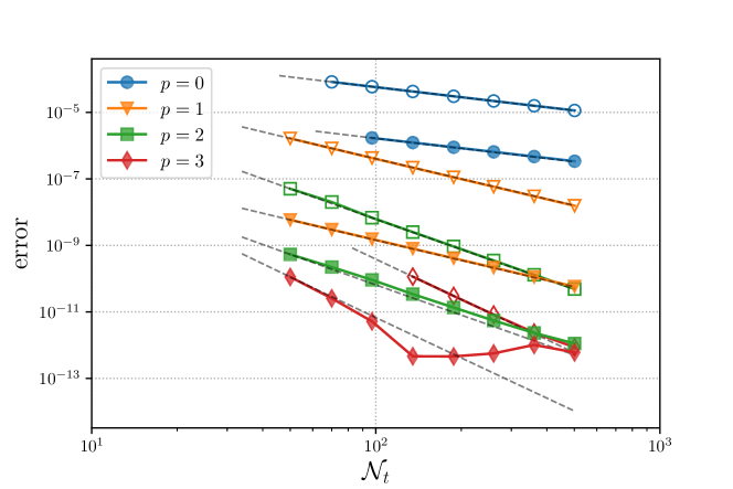
Figure 4.1: Plots of error vs. $\mathcal{N}_{t}$ for the multi-domain strategy with coupling at fixed intervals. Errors corresponding to the explicit and implicit coupling are shown with empty and filled markers, respectively. The dashed lines represent the theoretical accuracy ($\mathcal{O}(\Delta t_{c}^{p+1})$) for an approximation polynomial of degree $p$.

In Figure 4.1, the coupling errors from the above simulations are plotted against the number of coupling intervals on a log-log scale. The slopes of these curves represent the order of accuracy of the multi-domain method. Each of these curves corresponds to a specific degree of the approximation polynomial and either of the two coupling strategies. We observe that for a given coupling step size, the implicit coupling always has lower errors than the explicit coupling strategy. We can explain this by looking at the consistency loops of the implicit strategy. Except for the first iteration, interpolation instead of extrapolation is used to approximate the coupling variables. The error constant is smaller for interpolation than that of extrapolation resulting in smaller errors for the implicit coupling strategy. Note that for the consistency loops, we keep $\mathrm{WR}_{tol}=\mathrm{1\times 10^{-10}}$, which is sufficiently low to ensure that the polynomial approximations of the coupling variables dominate the source of coupling error.

Moreover, the error curves satisfy the theoretical order curves given by Equation 3.4. Thus, we can safely conclude that the theoretical accuracy of coupling is verified for the 1D LIB problem represented by a system of DAEs. It is worth mentioning that this accuracy had only been verified previously for problems involving coupled subsystems of ODEs in the litterature. Upon this verification, we can confidently use the strategy of Sub-Section 3.3 to evaluate the adaptive coupling step size of the multi-domain method proposed for 1D LIB simulations.

4.2 Adaptive coupling for oscillating operating condition

To test the adaptive coupling strategy, we consider a test case involving an the application of an oscillating voltage on our 1D LIB model, thus inducing temporal oscillations of the coupling variables. We take a sine wave signal for the applied voltage with the mean voltage $U_{\rm{mean}}=$ 0.103 V $\approx U_{0}(c_{s,\rm{I}})$. It is chosen such that the LIB cell switches between the charging and discharging modes during each oscillation of the voltage signal. This signal consists of three oscillations with an amplitude equal to 5% of the mean voltage. The adaptive coupling simulations are performed with a tolerance $tol=\mathrm{1\times 10^{-5}}$ on the error estimate for the optimal coupling step size. Similar to 4.1 each subdomain is discretised with 100 cells for the multi-domain simulations with adaptive coupling.

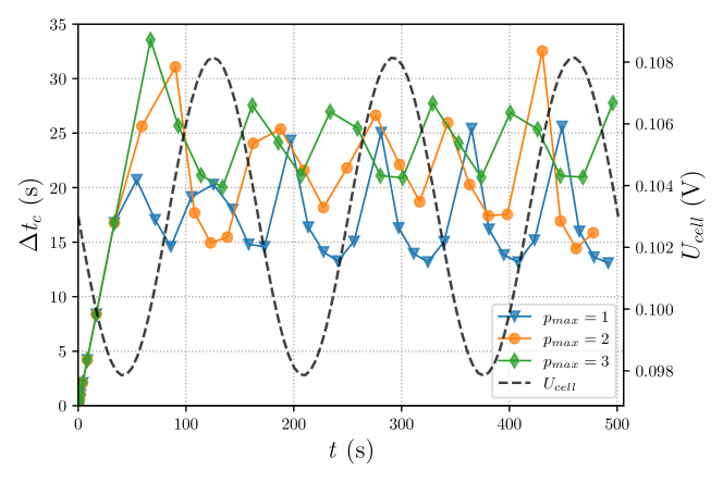
Figure 4.2: Plots of the coupling step $\Delta t_{c}$ (s) vs. time $t$ (s) for the multi-domain technique with adaptive coupling. Here $p_{max}$ is the highest degree of the approximation polynomials used for error estimation. The time-varying (sine wave) applied cell voltage is shown with the dashed line.

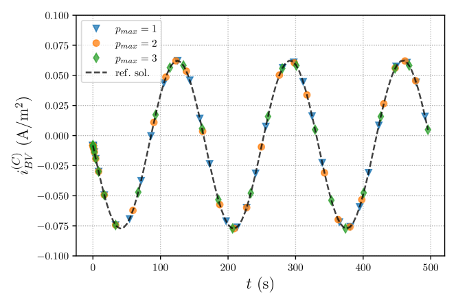
Figure 4.3: The temporal evolution curves of the Butler-Volmer current density at $\Gamma_{am-e}$ ($i_{BV}^{(C)}$), evaluated from the simulations using the multi-domain method with adaptive coupling for various coupling orders. For the monolithic reference solution $i_{BV}^{(C)}$ vs. $t$ is shown with dashed line.

In Figure 4.2, we plot the temporal evolutions of the adaptive coupling step $\Delta t_{c}$ for various orders of the adaptive coupling $p_{max}$. We observe that $\Delta t_{c}$ adapts well with the rate of change in the coupling dynamics, which is analogous to the $U_{cell}$ signal. At the beginning of the simulations, until $t\sim$ 35 s, the $\Delta t_{c}$ is gradually increased with a safety factor to avoid any numerical instabilities (ensuring that the error is always below the tolerance). We observe that the simulations with a higher order of coupling have larger coupling steps, i.e. for $p_{max}=\{\mathrm{1,\ 3}\}$ the maximum is $\Delta t_{c}=\{\mathrm{25.62~{}s,\ 33.55~{}s}\}$, respectively. It may be feared that the larger coupling steps can result in a loss of accuracy. However, in the present numerical strategy, we ensure that the coupling error, which in turn governs the global error of the simulations, is strictly controlled by the error estimate. Hence, the overall accuracy is maintained even for the larger coupling steps. We can demonstrate this by comparing the evolution of the Butler-Volmer current density at $\Gamma_{am-e}$ ($i_{BV}^{(C)}$) in Figure 4.3. For all $p_{max}$ values, there is a good match ($\mathrm{rel.\ error}\approx tol$) between the simulations with the adaptive coupling and the reference quasi-exact solution. The value of $i_{BV}^{(C)}$ oscillates between positive and negative values indicating the alternating charging and discharging modes of the LIB cell. We also observe that the applied voltage and the interface current density (in Figures 4.2 and 4.3, respectively) are in phase, confirming the absence of capacitive or inductive effects from the mathematical model.

4.3 Computational performance

In this last study, we use work-precision diagrams to analyze the computational performance of the adaptive coupling strategy implemented in this work. These diagrams, shown in Figures 4.5 and 4.4, plot the $\mathtt{CPU}\mathrm{time}$ of the simulations versus their errors evaluated by Equation 4.1 for the different orders of coupling $p_{max}$. For each order, the corresponding curve is obtained by performing multiple simulations with decreasing values of the coupling error tolerance. For each simulation, the error is then computed with respect to a quasi-exact monolithic solution, as in Sub-Section 4.1. In general, for a given error level, we observe a reduction in $\mathtt{CPU}\mathrm{time}$ when the order is increased. This is due to the larger coupling steps that higher-order coupling can take. For almost all tested configurations, as we move toward lower simulation errors, higher-order coupling leads to improved performance. The consistency of our observations in this 1D setup suggest the high potential of the proposed numerical strategy for 2D and 3D simulations as well.

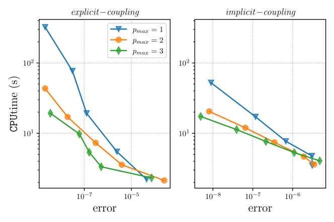
Figure 4.4: Work-precision diagram for the multi-domain method (constant voltage operation)

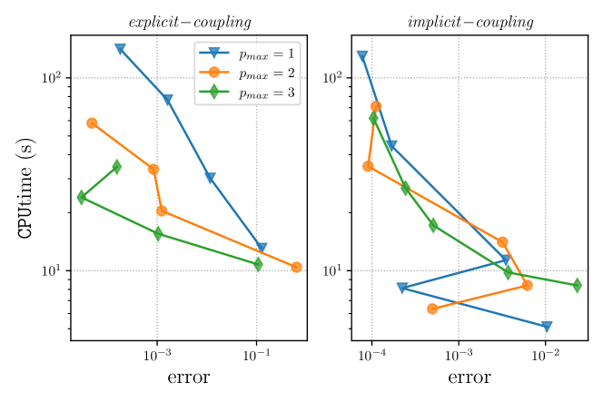
Figure 4.5: Work-precision diagram for the multi-domain method (sine wave oscillating voltage operation)

5 Conclusion

In this study, we have numerically solved a microscale continuum model of LIBs using the finite volume method and an adaptive multi-domain time integration strategy. This choice is motivated by the several orders of magnitude difference in the diffusion time scales characterizing the electrolyte and active material domains. The main nonlinearity of the problem arises at the solid-electrolyte interface due to the Butler-Volmer condition modeling the heterogeneous redox reactions. In the discretized system, we introduce auxiliary variables at this interface resulting in a nonlinear Robin condition. Consequently, the subproblem within each domain consists of a stiff system of DAEs that is solved by the implicit Radau5 method. The multi-domain approach allows to solve each subproblem independently, while the coupling between the domains is handled by a high-order adaptive coupling scheme.

Our numerical tests have shown that the accuracy of the multi-domain method is governed by the polynomial degree used in the approximation of the coupling variables, and that the adaptive coupling method remains stable even for an oscillating applied voltage at the LIB cell boundaries. Furthermore, higher-order coupling results in larger coupling steps, thus reducing the overall computational cost for a desired simulation accuracy.

The results of this 1D study motivate the future implementation of our numerical strategy in more realistic LIB simulations based on 3D electrode microstructures. However, such structures exhibit spatial multiscale features that require a fully adaptive time-space method. Numerical aspects like efficient nonlinear solvers for large systems of DAEs (such as ESDIRK method), better preconditioners for the linear solvers, parallelization and related HPC challenges need to be studied in the context of 3D LIB simulations. However, the proposed method can still be envisioned as a breakthrough for these applications in optimizing the coupling timestep for a given accuracy of the solution, while allowing a much better conditioning of the subproblems as illustrated in the supplementary material. Eventually, the multi-domain method offers a suitable framework for the LIB model extension to more complex physics, such as phase transformations and mechanical deformations in the active material, or lithium plating and SEI growth at the solid-electrolyte interface.

Table 5.1: Summary of constants and parameters.

Quantity	Value	Unit
F	96487	C$\cdot$mol-1
R	8.314	J$\cdot$(K$\cdot$mol)-1
T	298.15	K
$L_{e}$	20	$\mu$m
$c_{e,\rm{I}}$	1000	mol$\cdot$m-3
$D_{e}$	1$\times$10-10	m${}^{2}\cdot$s-1
$\kappa_{e}$	1	S$\cdot$m-1
$t_{+}^{0}$	0.4	dimensionless
$\delta_{e}$	0	dimensionless
$L_{am}$	10	$\mu$m
$c_{s,\rm{I}}$	13000	mol$\cdot$m-3
$D_{am}$	3$\times$10-14	m${}^{2}\cdot$s-1
$\sigma_{am}$	100	S$\cdot$m-1
$Fk_{0}$	8.9$\times$10-7	C$\cdot$s${}^{-1}\cdot$m${}^{2.5}\cdot$mol-1.5
$U_{0}({c}_{s})$	See Table 2 of [32]	V
$i_{0,\rm{Li}}$	10	C$\cdot$m${}^{-2}\cdot$s-1
$L_{cc}$	10	$\mu$m
$\sigma_{cc}$	3700	S$\cdot$m-1

Table 5.2: Summary of characteristic scales.

${\Phi}^{\star}$	$RT/F$	V
${L}^{\star}$	$L_{e}+L_{am}+L_{cc}=L$	m
${T}^{\star}$	$L^{2}/D_{e}$	s
${c}^{\star}_{e}$	$c_{e,\rm{I}}$	mol$\cdot$m-3
${c}^{\star}_{s}$	$c_{s,\rm{max}}$	mol$\cdot$m-3
${N}^{\star}_{e}$	$(D_{e}{c}^{\star}_{e})/{L}^{\star}$	mol$\cdot$m${}^{-2}\cdot$s-1
${i}^{\star}_{e}$	$(\kappa_{e}{\Phi}^{\star})/{L}^{\star}$	C$\cdot$m${}^{-2}\cdot$s-1
${N}^{\star}_{s}$	$(D_{am}{c}^{\star}_{s})/{L}^{\star}$	mol$\cdot$m${}^{-2}\cdot$s-1
${i}^{\star}_{s}$	$(\sigma_{am}{\Phi}^{\star})/{L}^{\star}$	C$\cdot$m${}^{-2}\cdot$s-1

Appendix A Verification of the mathematical model

Here we verify our numerical implementation of the 1D LIB half-cell model by considering a constant current (CC) charge scenario at 0.5C rate. The simulation is performed on a 1D finite volume grid of size $\mathcal{N}=200$. We employ a monolithic time integration method with the Radau5 solver relative tolerance set to $\mathrm{1\times 10^{-10}}$. Our results are compared to the reference battery simulator BESTmicro [16], using the same physical parameters and grid size. Moreover, numerical results are compared to an analytical solution that we have derived for the CC mode of operation (cf. Appendix C).

In Figure A.1, we plot the temporal evolutions of cell voltage ($U_{cell}$) obtained with our LIB model implementation, BESTmicro, and the analytical solution. Further, in Figure A.2, the spatial solution profiles are displayed at $t=$ 0 s and $t=$ 500 s for the three cases. These two figures illustrate the good agreement between the solutions, both in time and space. Therefore, this benchmark allows us to verify our implementation.

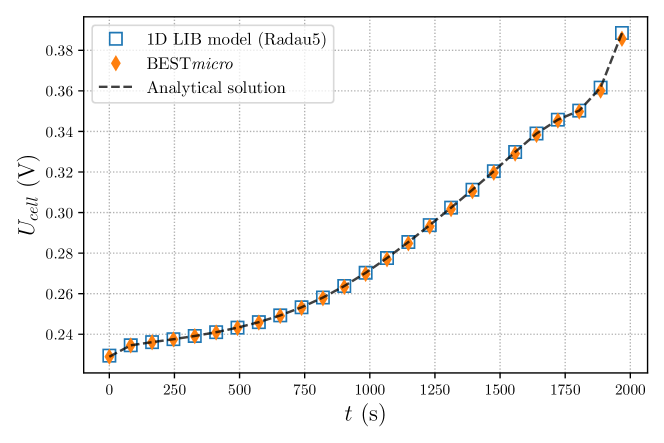
Figure A.1: Cell voltage versus time during CC charging at 0.5C rate, obtained from our numerical implementation (current study), BESTmicro, and analytical solution.

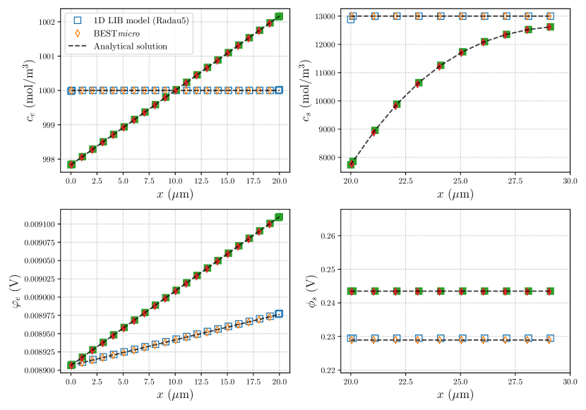
Figure A.2: Solution profiles in electrolyte (left panel) and active material (right panel) for CC charging at 0.5C rate, obtained from our numerical implementation (current study) and BESTmicro. The curves with empty and filled markers represent solutions at $t=$ 0 s and at $t=$ 500 s, respectively. The dashed lines show the corresponding analytical solution profiles.

Appendix B Space convergence study

Using a grid convergence study, we can verify the accuracy of the finite volume discretization. We analyze the spatial accuracies of lithium concentrations in the electrolyte and solid domains for a charging scenario at 1C rate. We also study the accuracy of the ionic potential in the electrolyte. For the electric potential, as we can see in Figure B.1, the piecewise linear nature of its solution profiles remains unchanged with time. Only the vertical intercepts (i.e., $\phi_{s}(L_{e},t)$) of these profiles evolve in time due to the variation of the auxiliary electric potential at $\Gamma_{am-e}$. Therefore, we have excluded the electric potential in the solid from this convergence study.

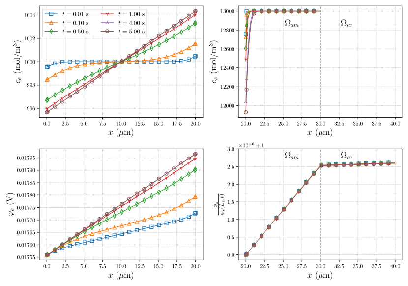
Figure B.1: Solution profiles in electrolyte (left panel) and active material (right panel) at various times during CC charging at 1C rate, obtained from our numerical implementation (current study).

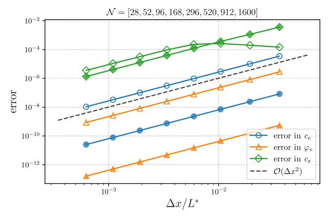
Figure B.2: Space convergence plots with errors between the numerical and analytical solutions for charging in CC mode at 1C rate evaluated at $t=$ 0.1 s (empty markers) and $t=$ 5 s (filled markers).

We perform several simulations with increasing $\mathcal{N}$, i.e., decreasing the 1D cell width $\Delta x$. The spatial integration error is evaluated as

$${\rm{error}}=\frac{\left\lVert y_{\rm{sim}}-y_{\rm{ref}}\right\rVert_{2}}{\left\lVert y_{\rm{ref}}\right\rVert_{2}}$$ (B.1)

where $\left\lVert\cdot\right\rVert_{2}$ is $\ell^{2}$-norm. Here $y_{\rm{sim}}$ and $y_{\rm{ref}}$ are the numerical and analytical solution profiles, respectively, both evaluated at the same reference time. We use sufficiently strict tolerances for time integration using the Radau5 method such that the temporal discretization errors remain negligible compared to the errors evaluated using Equation B.1.

In Figure B.2, the errors in concentrations and potentials are displayed as a function of dimensionless cell width on a log-log scale. The errors are evaluated from solutions at $t=$ 0.1 s and $t=$ 5 s corresponding to the transient and stationary states of the electrolyte, respectively. We observe that all the curves are parallel to the theoretical second-order curve. However, the spatial errors in ${c}_{s}$ at $t=$ 0.1 s are contaminated at larger $\Delta x$, most probably by higher-order terms in the Taylor expansion. These higher-order terms may become significantly large at early times due to the steep spatial gradients of ${c}_{s}$ near $\Gamma_{am-e}$. Nonetheless, we confirm the second order of convergence in space expected from the truncation error of the central difference scheme used in the spatial discretization.

Appendix C Analytical solution

In the particular scenario of a constant current (CC) charge or discharge, an analytical solution of the 1D LIB half-cell model can be obtained. The starting point of the derivation is to observe that the current densities in the electrolyte and solid phases remain constant and are both equal to the imposed current on $\Gamma_{L}$, $i_{\rm ext}=-\xi i_{1C}$. Thus, the electrolyte and solid-phase concentrations are effectively decoupled, each one satisfying a linear diffusion equation with constant Neumann conditions. The next steps of the derivation are summarized below, using the dimensional notations of Sub-Section 2.1.

C.1 Electrolyte concentration and potential

Electrolyte concentration satisfies the following initial value problem with Neumann boundary conditions,

$$\frac{\partial{c}_{e}}{\partial t} = D_{e}\frac{\partial^{2}{c}_{e}}{\partial x^{2}}\ ,$$ (C.1)

$$\frac{\partial{c}_{e}}{\partial x}(0,t) = \frac{\partial{c}_{e}}{\partial x}(L_{e},t)=-\beta_{e}\ ,$$ (C.2)

$${c}_{e}(x,0) = c_{e,\rm{I}}\ ,$$ (C.3)

where

$$\beta_{e}=\left(\frac{1-t_{+}^{0}}{FD_{e}}\right)i_{\rm ext}\ .$$ (C.4)

Applying the method of separation of variables, we obtain

$${c}_{e}(x,t) =c_{e,\rm{I}}+\beta_{e}\left(\frac{L_{e}}{2}-x\right)$$ (C.5)

$$\quad-4\beta_{e}L_{e}\sum_{k=0}^{\infty}\frac{1}{(2k+1)^{2}\pi^{2}}\cos\left(\frac{(2k+1)\pi x}{L_{e}}\right)e^{-\left(\frac{(2k+1)\pi}{L_{e}}\right)^{2}D_{e}t}\ .$$

Electrolyte potential satisfies a first-order ODE, obtained by taking the dot product of $\mathbf{i}_{e}$ from Equation 2.2 with the 1D normal vector $\mathbf{e}_{x}$, and then imposing ${\mathbf{i}}_{e}\cdot\mathbf{e}_{x}=i_{\rm ext}$. Further, at $x=0$ the Butler-Volmer condition Equation 2.8 yields ${\varphi}_{e}(0,t)=\frac{2RT}{F}\mathrm{argsh}\left(\frac{-i_{\rm ext}}{2i_{0,\rm Li}}\right)$. By integrating the ODE between $x=0$ and an arbitrary $x$, we obtain

$${\varphi}_{e}(x,t)=\frac{2RT}{F}\mathrm{argsh}\left(\frac{-i_{\rm ext}}{2i_{0,\rm Li}}\right)+\frac{2RT(1-t_{+}^{0})}{F}\ln\left(\frac{c_{e}(x,t)}{c_{e}(0,t)}\right)-\left(\frac{i_{\rm ext}}{\kappa_{e}}\right)x\ .$$ (C.6)

C.2 Solid-phase concentration

Let ${\bar{c}}_{s}(\bar{x},t)={c}_{s}(L_{e}+\bar{x},t)$ denote the solid-phase concentration in $\Omega_{am}$, expressed in terms of the shifted coordinate $\bar{x}=x-L_{e}$. This concentration satisfies the following initial value problem with Neuman boundary conditions,

$$\frac{\partial{\bar{c}}_{s}}{\partial t} = D_{am}\frac{\partial^{2}{\bar{c}}_{s}}{\partial\bar{x}^{2}}\ ,$$ (C.7)

$$\frac{\partial{\bar{c}}_{s}}{\partial\bar{x}}(0,t) = -\beta_{s}\ ,$$ (C.8)

$$\frac{\partial{\bar{c}}_{s}}{\partial\bar{x}}(L_{am},t) = 0\ ,$$ (C.9)

$${\bar{c}}_{s}(\bar{x},0) = c_{s,\rm{I}}\ ,$$ (C.10)

where

$$\beta_{s}=\left(\frac{1}{FD_{am}}\right)i_{\rm ext}\ .$$ (C.11)

Applying the method of separation of variables, we obtain

$${\bar{c}}_{s}(\bar{x},t) =c_{s,\rm{I}}-\beta_{s}\bar{x}\left(1-\frac{\bar{x}}{2L_{am}}\right)+\frac{\beta_{s}D_{am}\,t}{L_{am}}$$ (C.12)

$$\quad+2\beta_{s}L_{am}\left(\frac{1}{6}-\sum_{n=1}^{\infty}\frac{1}{n^{2}\pi^{2}}\cos\left(\frac{n\pi\bar{x}}{L_{am}}\right)e^{-\left(\frac{n\pi}{L_{am}}\right)^{2}D_{am}t}\right)\ .$$

C.3 Solid-phase potential and cell voltage

Let $c_{s}^{*}(t)$ and $\phi_{s}^{*}(t)$ denote the solid-phase variables at $\Gamma_{am-e}$, i.e., $c_{s}^{*}(t)={c}_{s}(L_{e},t)$ and $\phi_{s}^{*}(t)={\phi}_{s}(L_{e},t)$. Similarly, let $c_{e}^{*}(t)={c}_{e}(L_{e},t)$ and $\varphi_{e}^{*}(t)={\varphi}_{e}(L_{e},t)$. Further, we define the cell voltage as $U(t)={\phi}_{s}(L,t)$. Observing that the solid-phase potential is a continuous and piecewise linear function of $x$ (with constant slopes in $\Omega_{am}$ and $\Omega_{cc}$), we have

$$U(t) =\phi_{s}^{*}(t)-\left(\frac{L_{am}}{\sigma_{am}}+\frac{L_{cc}}{\sigma_{cc}}\right)i_{\rm ext}\ .$$ (C.13)

Finally, using the Butler-Volmer equation Equation 2.9, we obtain

$$\phi_{s}^{*}(t) =\varphi_{e}^{*}(t)+U_{0}(c_{s}^{*}(t))+\frac{2RT}{F}\mathrm{argsh}\left(\frac{-i_{\rm ext}}{2Fk_{0}\sqrt{c_{e}^{*}(t)c_{s}^{*}(t)\left(c_{s,\rm{max}}-c_{s}^{*}(t)\right)}}\right)\ ,$$ (C.14)

where $c_{e}^{*}(t)$, $\varphi_{e}^{*}(t)$ and $c_{s}^{*}(t)$ can be evaluated from Equation C.5, Equation C.6 and Equation C.12, respectively.

Appendix D Conditioning of the Jacobian system

One of the motivations to use multi-domain methods is to improve the conditioning of the Jacobian system by decoupling the two diffusion time scales. In this study, we evaluate and compare the condition numbers of the Jacobian matrices $J_{\rm full}(W,Z)$, $J_{e}(W_{e},Z_{e})$, and $J_{s}(W_{s},Z_{s})$, corresponding to residual functions of the fully-coupled system and to each subproblem (electrolyte and solid), respectively. In this study, we have numerically evaluated these Jacobian matrices for the residual functions obtained from the implementation of Radau5 time integration method.

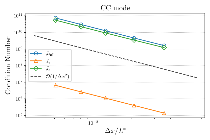
Figure D.1: Conditioning of Jacobian matrices $J_{\rm full}$, $J_{e}$, and $J_{s}$, evaluated at $t=\mathrm{101\ s}$ for solutions in CC mode at 1C rate.

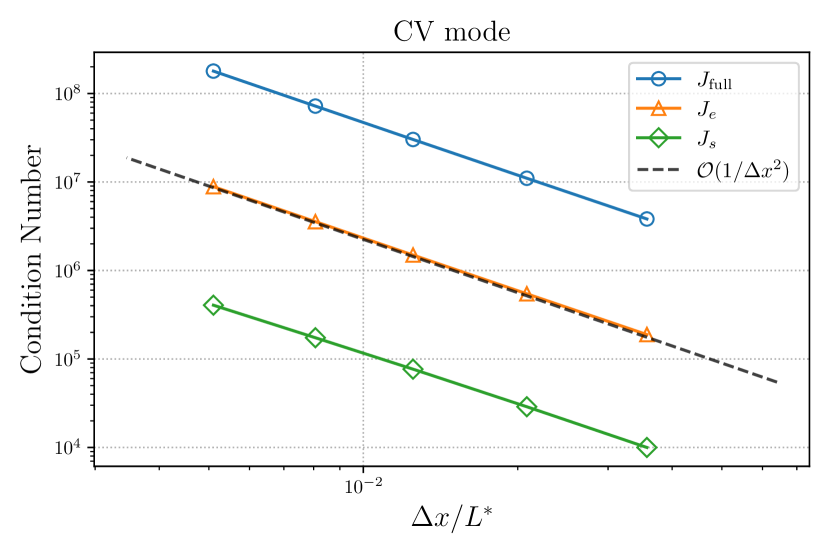
Figure D.2: Conditioning of Jacobian matrices $J_{\rm full}$, $J_{e}$, and $J_{s}$, evaluated at $t=\mathrm{101\ s}$ for solutions in CV mode at 0.103 V.

In Figures D.1 and D.2, the condition numbers of $J_{\rm full}$, $J_{e}$, and $J_{s}$ are plotted at the final simulation time $t=\mathrm{101\ s}$ with respect to nondimensional cell width, for CC and CV modes of operation, respectively. It should be noted that these condition numbers are almost independent of the temporal evolution of the solution. The plots follow the theoretical order expected from the discretization of the diffusion-based governing equations.

In the CC mode, the ill-conditioning of $J_{s}$ is still comparable to that of the fully-coupled Jacobian $J_{\rm full}$. The constant Butler-Volmer current results in Neumann-type boundary conditions on both sides of the solid domain making $J_{s}$ nearly singular. While in CV mode, we observe a significant reduction in condition numbers of both $J_{e}$ and $J_{s}$. Such improvements in conditioning are advantageous in the context of iterative linear solvers, to reduce the number of iterations and thus the computational cost.

References

- [1] J. M. Allen, J. Chang, F. L. E. Usseglio-Viretta, P. Graf, and K. Smith, A Segregated Approach for Modeling the Electrochemistry in the 3-D Microstructure of Li-Ion Batteries and Its Acceleration Using Block Preconditioners, Journal of Scientific Computing, 86 (2021).
- [2] H. Arunachalam, S. Onori, and I. Battiato, On veracity of macroscopic lithium-ion battery models, Journal of The Electrochemical Society, 162 (2015), p. A1940.
- [3] A. Bartlett, J. Marcicki, S. Onori, G. Rizzoni, X. G. Yang, and T. Miller, Electrochemical model-based state of charge and capacity estimation for a composite electrode lithium-ion battery, IEEE Transactions on control systems technology, 24 (2015), pp. 384–399.
- [4] C. Batchelor-McAuley, E. Kätelhön, E. O. Barnes, R. G. Compton, E. Laborda, and A. Molina, Recent Advances in Voltammetry, ChemistryOpen, 4 (2015), pp. 224–260.
- [5] A. F. Bower, P. R. Guduru, and V. A. Sethuraman, A finite strain model of stress, diffusion, plastic flow, and electrochemical reactions in a lithium-ion half-cell, Journal of the Mechanics and Physics of Solids, 59 (2011), pp. 804–828.
- [6] K. E. Brenan, S. L. Campbell, and L. R. Petzold, Numerical Solution of Initial-Value Problems in Differential-Algebraic Equations, Society for Industrial and Applied Mathematics, 1995.
- [7] G. F. Castelli and W. Dörfler, The numerical study of a microscale model for lithium-ion batteries, Computers & Mathematics with Applications, 77 (2019), pp. 1527–1540.
- [8] COMSOL, Battery Design Module, 2010.
- [9] D. Di Domenico, A. Stefanopoulou, and G. Fiengo, Lithium-ion battery state of charge and critical surface charge estimation using an electrochemical model-based extended kalman filter, Journal of dynamic systems, measurement, and control, 132 (2010).
- [10] M. Doyle and J. Newman, The use of mathematical modeling in the design of lithium/polymer battery systems, Electrochimica Acta, 40 (1995), pp. 2191–2196.
- [11] M. Duarte, M. Massot, S. Descombes, C. Tenaud, T. Dumont, V. Louvet, and F. Laurent, New resolution strategy for multiscale reaction waves using time operator splitting, space adaptive multiresolution, and dedicated high order implicit/explicit time integrators, SIAM Journal on Scientific Computing, 34 (2012), pp. A76–A104.
- [12] R. Eymard, T. Gallouët, and R. Herbin, Finite volume methods, in Solution of Equation in (Part 3), Techniques of Scientific Computing (Part 3), vol. 7 of Handbook of Numerical Analysis, Elsevier, 2000, pp. 713–1018.
- [13] R. Fang, P. Farah, A. Popp, and W. A. Wall, A monolithic, mortar-based interface coupling and solution scheme for finite element simulations of lithium-ion cells, International Journal for Numerical Methods in Engineering, 114 (2018), pp. 1411–1437.
- [14] R. Fang, M. Kronbichler, M. Wurzer, and W. A. Wall, Parallel, physics-oriented, monolithic solvers for three-dimensional, coupled finite element models of lithium-ion cells, Computer Methods in Applied Mechanics and Engineering, 350 (2019), pp. 803–835.
- [15] M. E. Ferraro, B. L. Trembacki, V. E. Brunini, D. R. Noble, and S. A. Roberts, Electrode Mesoscale as a Collection of Particles: Coupled Electrochemical and Mechanical Analysis of NMC Cathodes, Journal of The Electrochemical Society, 167 (2020), p. 013543.
- [16] F. I. for Industrial Mathematics ITWM, BESTmicro Battery and Electrochemistry Simulation Tool - Fraunhofer ITWM, 2018.
- [17] L. Francois, Multiphysical modelling and simulation of the ignition transient of complete solid rocket motors, these de doctorat, Institut polytechnique de Paris, Feb. 2022.
- [18] T. F. Fuller, M. Doyle, and J. Newman, Simulation and Optimization of the Dual Lithium Ion Insertion Cell, Journal of The Electrochemical Society, 141 (1994), p. 1.
- [19] G. M. Goldin, A. M. Colclasure, A. H. Wiedemann, and R. J. Kee, Three-dimensional particle-resolved models of li-ion batteries to assist the evaluation of empirical parameters in one-dimensional models, Electrochimica Acta, 64 (2012), pp. 118–129.
- [20] E. Hairer and G. Wanner, Solving Ordinary Differential Equations II, Springer Berlin, Heidelberg, 2 ed., Sept. 1996.
- [21] S. Hein, T. Danner, and A. Latz, An electrochemical model of lithium plating and stripping in lithium ion batteries, ACS Applied Energy Materials, 3 (2020), pp. 8519–8531.
- [22] T. Hofmann, R. Müller, H. Andrä, and J. Zausch, Numerical simulation of phase separation in cathode materials of lithium ion batteries, International Journal of Solids and Structures, 100 (2016), pp. 456–469.
- [23] T. Hutzenlaub, S. Thiele, N. Paust, R. Spotnitz, R. Zengerle, and C. Walchshofer, Three-dimensional electrochemical Li-ion battery modelling featuring a focused ion-beam/scanning electron microscopy based three-phase reconstruction of a LiCoO2 cathode, Electrochimica Acta, 115 (2014), pp. 131–139.
- [24] O. Iliev, M. A. Nikiforova, Y. V. Semenov, and P. E. Zakharov, Splitting algorithm for numerical simulation of Li-ion battery electrochemical processes, AIP Conference Proceedings, 1907 (2017), p. 030019.
- [25] O. Iliev and P. E. Zakharov, Domain splitting algorithms for the Li-ion battery simulation, IOP Conference Series: Materials Science and Engineering, 158 (2016), p. 012099.
- [26] A. G. Kashkooli, S. Farhad, D. U. Lee, K. Feng, S. Litster, S. K. Babu, L. Zhu, and Z. Chen, Multiscale modeling of lithium-ion battery electrodes based on nano-scale X-ray computed tomography, Journal of Power Sources, 307 (2016), pp. 496–509.
- [27] A. Kværnø, Singly Diagonally Implicit Runge–Kutta Methods with an Explicit First Stage, BIT Numerical Mathematics, 44 (2004), pp. 489–502.
- [28] A. Latz and J. Zausch, Thermodynamic consistent transport theory of Li-ion batteries, Journal of Power Sources, 196 (2011), pp. 3296–3302.
- [29] A. Latz and J. Zausch, Multiscale modeling of lithium ion batteries: thermal aspects, Beilstein Journal of Nanotechnology, 6 (2015), pp. 987–1007.
- [30] G. B. Less, J. H. Seo, S. Han, A. M. Sastry, J. Zausch, A. Latz, S. Schmidt, C. Wieser, D. Kehrwald, and S. Fell, Micro-Scale Modeling of Li-Ion Batteries: Parameterization and Validation, Journal of The Electrochemical Society, 159 (2012), p. A697.
- [31] B. Y. Liaw, G. Nagasubramanian, R. G. Jungst, and D. H. Doughty, Modeling of lithium ion cells—a simple equivalent-circuit model approach, Solid state ionics, 175 (2004), pp. 835–839.
- [32] W. Mai, F. L. Usseglio-Viretta, A. M. Colclasure, and K. Smith, Enabling fast charging of lithium-ion batteries through secondary-/dual- pore network: Part ii - numerical model, Electrochimica Acta, 341 (2020), p. 136013.
- [33] S. Müller, J. Eller, M. Ebner, C. Burns, J. Dahn, and V. Wood, Quantifying inhomogeneity of lithium ion battery electrodes and its influence on electrochemical performance, Journal of The Electrochemical Society, 165 (2018), p. A339.
- [34] A. Muralidharan, M. I. Chaudhari, L. R. Pratt, and S. B. Rempe, Molecular Dynamics of Lithium Ion Transport in a Model Solid Electrolyte Interphase, Scientific Reports, 8 (2018), p. 10736.
- [35] J. Newman and N. P. Balsara, Electrochemical systems, John Wiley & Sons, 2021.
- [36] P. Popov, Y. Vutov, S. Margenov, and O. Iliev, Finite Volume Discretization of Equations Describing Nonlinear Diffusion in Li-Ion Batteries, in Numerical Methods and Applications, I. Dimov, S. Dimova, and N. Kolkovska, eds., Lecture Notes in Computer Science, Berlin, Heidelberg, 2011, Springer, pp. 338–346.
- [37] S. Psaltis and T. Farrell, Comparing charge transport predictions for a ternary electrolyte using the Maxwell-Stefan and Nernst-Planck equations, Journal of the Electrochemical Society, 158 (2011), pp. A33–A42.
- [38] E. K. Rahani and V. B. Shenoy, Role of Plastic Deformation of Binder on Stress Evolution during Charging and Discharging in Lithium-Ion Battery Negative Electrodes, Journal of The Electrochemical Society, 160 (2013), p. A1153.
- [39] S. A. Roberts, V. E. Brunini, K. N. Long, and A. M. Grillet, A Framework for Three-Dimensional Mesoscale Modeling of Anisotropic Swelling and Mechanical Deformation in Lithium-Ion Electrodes, Journal of The Electrochemical Society, 161 (2014), p. F3052.
- [40] F. Schneider, J. Zausch, J. Lammel, and H. Andrä, An efficient semi-implicit solver for solid electrolyte interphase growth in li-ion batteries, Applied Mathematical Modelling, 109 (2022), pp. 741–759.
- [41] Siemens Digital Industries Software, Simcenter STAR-CCM+, version 2021.1, 2021.
- [42] F. Single, B. Horstmann, and A. Latz, Dynamics and morphology of solid electrolyte interphase (SEI), Physical Chemistry Chemical Physics, 18 (2016), pp. 17810–17814.
- [43] M. Smith, R. E. García, and Q. C. Horn, The effect of microstructure on the galvanostatic discharge of graphite anode electrodes in licoo2-based rocking-chair rechargeable batteries, Journal of The Electrochemical Society, 156 (2009), p. A896.
- [44] R. Spotnitz, B. Kaludercic, S. Muzaferija, M. Peric, G. Damblanc, and S. Hartridge, Geometry-resolved electro-chemistry model of li-ion batteries, SAE International Journal of Alternative Powertrains, 1 (2012), pp. 160–168.
- [45] K. Takizawa and T. E. Tezduyar, Multiscale space–time fluid–structure interaction techniques, Computational Mechanics, 48 (2011), pp. 247–267.
- [46] T. E. Tezduyar and S. Sathe, Modelling of fluid–structure interactions with the space–time finite elements: Solution techniques, International Journal for Numerical Methods in Fluids, 54 (2007), pp. 855–900.
- [47] N. Xue, W. Du, J. R. Martins, and W. Shyy, Lithium-Ion Batteries: Thermomechanics, Performance, and Design Optimization, in Encyclopedia of Aerospace Engineering, John Wiley & Sons, Ltd, 2016, pp. 1–17.
- [48] S. Zhang, O. Iliev, S. Schmidt, and J. Zausch, Comparison of Two Approaches for Treatment of the Interface Conditions in FV Discretization of Pore Scale Models for Li-Ion Batteries, in Finite Volumes for Complex Applications VII-Elliptic, Parabolic and Hyperbolic Problems, J. Fuhrmann, M. Ohlberger, and C. Rohde, eds., Springer Proceedings in Mathematics & Statistics, Cham, 2014, Springer International Publishing, pp. 731–738.