Understanding black-box models with dependent inputs through a generalization of Hoeffding’s decomposition

Abstract

One of the main challenges for interpreting black-box models is the ability to uniquely decompose square-integrable functions of non-mutually independent random inputs into a sum of functions of every possible subset of variables. However, dealing with dependencies among inputs can be complicated. We propose a novel framework to study this problem, linking three domains of mathematics: probability theory, functional analysis, and combinatorics. We show that, under two reasonable assumptions on the inputs (non-perfect functional dependence and non-degenerate stochastic dependence), it is always possible to decompose uniquely such a function. This “canonical decomposition” is relatively intuitive and unveils the linear nature of non-linear functions of non-linearly dependent inputs. In this framework, we effectively generalize the well-known Hoeffding decomposition, which can be seen as a particular case. Oblique projections of the black-box model allow for novel interpretability indices for evaluation and variance decomposition. Aside from their intuitive nature, the properties of these novel indices are studied and discussed. This result offers a path towards a more precise uncertainty quantification, which can benefit sensitivity analyses and interpretability studies, whenever the inputs are dependent. This decomposition is illustrated analytically, and the challenges to adopting these results in practice are discussed.

1 Introduction

When dealing with complex black-box models (e.g., predictive models, numerical simulation codes) with non-deterministic inputs, assessing the effects of the random nature of the inputs on the output is paramount in many studies. This general problem has broad application in many fields, such as sensitivity analysis (SA) [10] and explainability in artificial intelligence (XAI) [1]. In particular, in industrial practices (e.g., when dealing with critical systems), uncertainty quantification (UQ) enables the improvement of the studied phenomenon modeling process and can allow for scientific discoveries [14].

One of the main challenges when it comes to UQ is to deal with dependent inputs. The proposed methods usually assume mutual independence of the inputs [53, 38], either for the simplicity of the resulting estimation schemes or for the lack of a proper framework. However, in practice, the inputs are often endowed with a dependence structure intrinsic to the (observed or modeled) studied phenomena. Always assuming mutual independence can be seen as expedient and can lead to improper insights [26]. One of the main challenges to a better understanding of black-box models is to take this dependence structure into account [45] and, above all, to formally justify the proposed methods without heavily relying on empirical observations or specific benchmarks.

One classical way to assess the effects of input uncertainties is using functional decompositions, obtaining so-called high-dimensional model representations (HDMR) [43]. Formally, for random inputs $X=(X_{1},\dots,X_{d})^{\top}$, and an output $G(X)$, it amounts to finding the unique decomposition

$$G(X)=\sum_{A\in\mathcal{P}_{D}}G_{A}(X_{A}),$$ (1)

where $D=\{1,\dots,d\}$, $\mathcal{P}_{D}$ is the set of subsets of $D$, and $G_{A}(X_{A})$ are functions of the subset of input $X_{A}=(X_{i})_{i\in A}$. Whenever the $X_{i}$ are assumed to be mutually independent, such a decomposition is known as Hoeffding’s decomposition, due to his seminal work on the subject [27]. Whenever the inputs are not assumed to be mutually independent, many approaches have been proposed in the literature. Notably, [26] proposed an approximation theoretic framework to address the problem, and provides useful tools for importance quantification, but they lack a proper and intuitive understanding of the quantities being estimated. On the one hand in [7], the authors approached the problem differently and brought forward an intuitive view on the subject, but under very limiting assumptions on the probabilistic structure of the inputs. On the other hand, [28] and [34] proposed a projection-based approach under constraints derived from desirability criteria. However, all of these approaches lack a clear framework or do not offer completely satisfactory answers to uncertainty quantification with dependent inputs. Other approaches rely on transforming the dependent inputs to achieve mutual independence using, e.g., Nataf or Rosenblatt transforms [36, 37, 40]. While these approaches can be applied to a broad range of probabilistic structures, they can be seen as lacking in generality (e.g., existence of probability density functions, being in an elliptical family of distribution). While they offer meaningful indications on the relationship between $X$ and $G(X)$, they do not quantify the effects due to the dependence.

To fill this gap, our article proposes a framework at the cornerstone of probability theory, functional analysis, and abstract algebra. By viewing random variables as measurable functions, we are able to show that a unique decomposition such as (1), for square-integrable black-box outputs $G(X)$, is indeed possible under two fairly reasonable assumptions on the inputs:

1. Non-perfect functional dependence;

2. Non-degenerate stochastic dependence.

To be more specific, denote $\sigma_{X}$ the $\sigma$-algebra generated by $X$, and $\mathbb{L}^{2}\left(\sigma_{X}\right)$ the space of square-integrable $\sigma_{X}$-measurable real-valued functions (i.e., real-valued functions of $X$). From the proposed framework, defining a decomposition such as in (1) equates to defining a direct-sum decomposition of $\mathbb{L}^{2}\left(\sigma_{X}\right)$ of the form

$$\mathbb{L}^{2}\left(\sigma_{X}\right)=\bigoplus_{A\in\mathcal{P}_{D}}V_{A},$$

where $V_{A}$ are some linear vector subspaces of functions of $X_{A}$. We show that such a decomposition exists and offers a complete definition of the subspaces $V_{A}$. Additionally, to the best of our knowledge, it offers a new way to approach multivariate dependence, relying on linear geometry. We also show that Hoeffding’s decomposition is a very special case of our framework, which ultimately generalizes this result. Moreover, it offers a way to better understand, comprehend, handle, and disentangle effects due to the internal dependence structure of $X$ and the interaction effects due to the model $G$. Based on this, novel indices are proposed, allowing decomposing evaluations (observations) of $G(X)$ and quantifying the influence of the inputs and their interactions within $G$ by decomposing its variance.

This document is organized as follows. Section 2 is dedicated to introducing the overall framework, notations, and the required preliminaries and key definitions to introduce our result. Section 3 is dedicated to the main result of this paper. This result is discussed, and a particular focus is put on the fact that it generalizes the known results in the situation of mutually independent inputs. Section 4 introduces novel decompositions for two quantities of interest: an evaluation of a model and its variance. The proposed indices are intuitive, disentangle interaction effects to effects due to the dependence, and allow for a novel way of quantifying uncertainties. Section 5 is dedicated to the illustration of our result in the particular case of a model with two Bernoulli inputs. In this illustration, the decomposition can be computed analytically, and the proposed indices also admit analytical formulas. Finally, Section 6 discusses the challenges for a broad acceptance of the proposed method in practice, as well as some motivating perspectives.

2 Notations and preliminaries

In the remainder of this document, the following notations are adopted. $\subset$ indicates a proper (strict) inclusion, while $\subseteq$ indicates a possible equality between sets. “Random variables” refer to real-valued random elements, and “random vector” refers to a vector of random variables. “Random element” is used if the domain of measurable functions is not necessarily real. Independence between random elements is denoted using $\perp\!\!\!\perp$. For a measurable space $(E,\mathcal{E})$ and $B\subset\mathcal{E}$, we denote by $\sigma\left[B\right]$ the smallest $\sigma$-algebra containing $B$. For a finite set $D=\{1,\dots,d\}$ for a positive integer $d$, denote $\mathcal{P}_{D}$ its power-set (i.e., the set of subsets of $D$, including $D$ and $\emptyset$), and for any $A\in\mathcal{P}_{D}$, denote $\mathcal{P}_{-A}=\mathcal{P}_{A}\setminus\{A\}$ (i.e., the power-set of $A$ without $A$). Depending on the context, when dealing with a set $A$, $\left|A\right|$ denotes its cardinality (i.e., the number of elements in $A$), while for a real $c\in\mathbb{R}$, $\left|c\right|$ denotes its absolute value.

2.1 Framework

Let $(\Omega,\mathcal{F},\mathbb{P})$ be a standard probability space, let $d\geq 1$ be a positive integer, and let $(E_{1},\mathcal{E}_{1}),\dots,(E_{d},\mathcal{E}_{d})$ be a collection of standard Borel measurable spaces. Let $D=\left\{1,\dots,d\right\}$ and denote $\mathcal{P}_{D}$ the power-set of $D$ (i.e., the set of subsets of $D$, including the empty set $\emptyset$). For every $A\in\mathcal{P}_{D},A\neq\emptyset$, denote:

$$E_{A}:=\bigtimes_{i\in A}E_{i},\quad\mathcal{E}_{A}:=\bigotimes_{i\in A}\mathcal{E}_{i},$$

where $\times$ denotes the Cartesian product between sets and $\otimes$ denotes the product of $\sigma$-algebras (see [39], Section 2.4.2). Notice additionally that $(E_{A},\mathcal{E}_{A})$ is also a standard Borel measurable space (see, e.g., [31], Lemma 1.2). Denote $E:=E_{D}$ and $\mathcal{E}:=\mathcal{E}_{D}$.

Let $X=\left(X_{1},\dots,X_{d}\right)^{\top}$ be an $E$-valued, $\mathcal{F}$-measurable function (i.e., a vector of random elements), which is referred to as the random inputs in the remainder of the paper. Moreover, for any $A\in\mathcal{P}_{D}$, denote $X_{A}:=\left(X_{i}\right)_{i\in A}$ the $E_{A}$-valued function, and notice that it is $\mathcal{F}$-measurable as well, and hence also forms a vector of random elements (see, e.g., [31] Lemma 1.9).

Denote by $\sigma_{\emptyset}$ the $\mathbb{P}$-trivial $\sigma$-algebra, defined as

$$\sigma_{\emptyset}:=\left\{A\in\mathcal{F}:\mathbb{P}\left(A\right)\in\left\{0,1\right\}\right\}$$

i.e., the smallest $\sigma$-algebra generated by the null sets w.r.t. $\mathbb{P}$ (see, e.g., [47], p.108). Moreover, for $i=1,\dots,d$, denote

$$\sigma_{i}:=\left\{X_{i}^{-1}(B),\forall B\in\mathcal{E}_{i}\right\}\subseteq\mathcal{F}$$

where $X_{i}^{-1}$ denotes the inverse image of $X_{i}$ (see, e.g., [39], Proposition 2.1.1). Denote by $\sigma_{X}$ the $\sigma$-algebra generated by $X$, defined as

$$\sigma_{X}:=\sigma\left[\bigcup_{i\in D}\sigma_{i}\right]=\left\{X^{-1}(B),\forall B\in\mathcal{E}\right\}\subseteq\mathcal{F},$$

and finally, for every $A\in\mathcal{P}_{D},A\not\in\left\{\emptyset,D\right\}$, $\sigma_{A}$ the $\sigma$-algebra generated by the subset of inputs $X_{A}$, defined as

$$\sigma_{A}:=\sigma\left[\bigcup_{i\in A}\sigma_{i}\right]=\left\{X_{A}^{-1}(B),\forall B\in\mathcal{E}_{A}\right\}\subseteq\mathcal{F}.$$

For every $A\in\mathcal{P}_{D},A\neq\emptyset$, denote by $P_{X_{A}}$ the probability measure induced by $X_{A}$, defined, $\forall B\in\mathcal{E}_{A}$, as,

$$P_{X_{A}}(B)=\mathbb{P}\left(X_{A}^{-1}(B)\right).$$

Denote $\mathbb{L}^{2}(\mathcal{F})$ the Lebesgue space of $\mathbb{R}$-valued square-integrable $\mathcal{F}$-measurable functions, and for any sub $\sigma$-algebra $\mathcal{G}\subseteq\mathcal{F}$, denote $\mathbb{L}^{2}\left(\mathcal{G}\right)$ the space of $\mathbb{R}$-valued square-integrable $\mathcal{G}$-measurable functions. Recall the following classical result ([52], Theorem 2).

Theorem 1.

For two sub $\sigma$-algebras $\mathcal{G}_{1}$ and $\mathcal{G}_{2}$ of $\mathcal{F}$, the following assertions hold.

1. If $\mathcal{G}_{1}\subset\mathcal{G}_{2}$, then $\mathbb{L}^{2}\left(\mathcal{G}_{1}\right)\subset\mathbb{L}^{2}\left(\mathcal{G}_{2}\right)$.

2. $\mathbb{L}^{2}\left(\mathcal{G}_{1}\right)\cap\mathbb{L}^{2}\left(\mathcal{G}_{2}\right)=\mathbb{L}^{2}\left(\mathcal{G}_{1}\cap\mathcal{G}_{2}\right)$.

Remark 1.

As the Lebesgue space $\mathbb{L}^{2}\left(\sigma_{\mathcal{F}}\right)$ is defined as the canonical quotient space between the $\mathbb{R}$-valued square-integrable $\mathcal{F}$-measurable functions and the set of functions equal to $0$ almost everywhere (a.e.), every equality between elements of $\mathbb{L}^{2}\left(\sigma_{\mathcal{F}}\right)$ stated in the following is to be understood as being almost sure (a.s.).

For any $A\in\mathcal{P}_{D},A\neq\emptyset$, notice that for any $Y\in\mathbb{L}^{2}\left(\sigma_{A}\right)$, one has that there exist a function $f:E_{A}\rightarrow\mathbb{R}$ such that $Y=f(X_{A})$ a.s., thanks to the Doob-Dynkin Lemma (see, e.g., [31], Lemma 1.14). Additionally, notice that $\mathbb{L}^{2}\left(\sigma_{\emptyset}\right)$ comprises constant a.s. functions ([47], Lemma 4.5.1). Let $G:E\rightarrow\mathbb{R}$ be a function representing a black-box model, such that the $\mathbb{R}$-valued random variable $G(X)$ is in $\mathbb{L}^{2}\left(\sigma_{X}\right)$. $G(X)$ is referred to as the random output in the remainder of this paper.

Remark 2.

This framework adopts a measure-theoretic point of view for the sake of generality. Taking the random inputs to be valued in a cartesian product of abstract Polish spaces is a way not to restrain them from being real-valued. In essence, the inputs can be valued in different types of spaces (e.g., images, functions, stochastic processes) as long as they are measurable.

2.2 Elements of linear algebra and functional analysis

2.2.1 Vector space direct sum

Let $W$ be a vector space, and $W_{1}$ and $W_{2}$ be two proper (linear vector) subspaces of $w$ (i.e., $W_{1}\neq W$, $W_{2}\neq W$). The sum between $W_{1}$ and $W_{2}$ is the vector subspace of $W$ defined as (see, e.g., [4], Definition 1.36):

$$W_{1}+W_{2}=\left\{w_{1}+w_{2}:w_{1}\in W_{1},w_{2}\in W_{2}\right\}.$$

$W_{1}$ and $W_{2}$ are said to be in direct sum if additionally $W_{1}\cap W_{2}=\{0_{W}\}$ (i.e., the zero vector of $W$), and the sum of the two subspaces is denoted $W_{1}\oplus W_{2}$ (see, e.g., [4], Proposition 1.45).

For a positive integer $n\geq 1$, let $W_{1},\dots,W_{n}$ be proper subspaces of $W$. If for every element $w$ of the subspace

$$\mathop{\mathchoice{\vbox{\hbox{\leavevmode\resizebox{}{9.00005pt}{\raisebox{0.0pt}{$\displaystyle+$}}}}\vphantom{\sum}}{\vbox{\hbox{\leavevmode\resizebox{}{9.00005pt}{\raisebox{0.0pt}{$\textstyle+$}}}}\vphantom{\sum}}{\vbox{\hbox{\leavevmode\resizebox{}{6.30003pt}{\raisebox{0.0pt}{$\scriptstyle+$}}}}\vphantom{\sum}}{\vbox{\hbox{\leavevmode\resizebox{}{4.50002pt}{\raisebox{0.0pt}{$\scriptscriptstyle+$}}}}\vphantom{\sum}}}\slimits@_{i=1}^{n}W_{i}:=\left\{\sum_{i=1}^{n}w_{i}:w_{i}\in W_{i},i=1,\dots,n\right\}$$

there exists only a unique set of elements $(w_{i})_{i=1,\dots,n},w_{i}\in W_{i}$ such that $w=\sum_{i=1}^{n}w_{i}$, then the subspaces are said to be in direct sum (see, e.g., [4], Definition 1.40), and the sum is denoted using the $\oplus$ symbol. Moreover, $W_{1},\dots,W_{n}$ are in direct sum (see, e.g., [4], Proposition 1.44) if and only if, for $\sum_{i=1}^{n}w_{i}\in\mathop{\mathchoice{\vbox{\hbox{\leavevmode\resizebox{}{9.00005pt}{\raisebox{0.0pt}{$\displaystyle+$}}}}\vphantom{\sum}}{\vbox{\hbox{\leavevmode\resizebox{}{9.00005pt}{\raisebox{0.0pt}{$\textstyle+$}}}}\vphantom{\sum}}{\vbox{\hbox{\leavevmode\resizebox{}{6.30003pt}{\raisebox{0.0pt}{$\scriptstyle+$}}}}\vphantom{\sum}}{\vbox{\hbox{\leavevmode\resizebox{}{4.50002pt}{\raisebox{0.0pt}{$\scriptscriptstyle+$}}}}\vphantom{\sum}}}\slimits@_{i=1}^{n}W_{i}$

$$\sum_{i=1}^{n}w_{i}=0\implies w_{i}=0,\quad i=1,\dots,n.$$

If additionally

$$W=\bigoplus_{i=1}^{n}W_{i},$$

then $W$ is said to be in a direct sum decomposition.

2.2.2 Hilbert spaces

A real Banach space is complete normed space, usually defined as a tuple $\left(\mathcal{M},\left\lVert.\right\rVert\right)$, where $\mathcal{M}$ is a vector space over the reals and $\left\lVert.\right\rVert:\mathcal{M}\rightarrow\mathbb{R}$ is a norm, with the added property that the limit of every converging sequence of elements of $\mathcal{M}$ (i.e., Cauchy sequences) is in $\mathcal{M}$ itself. Whenever the norm $\left\lVert.\right\rVert$ stems from an inner product $\left\langle.,.\right\rangle$, the resulting space is called a Hilbert space (see, e.g., [8], Definition 1.6). Hence, every Hilbert space is a Banach space [50].

Remark 3.

$\forall A\in\mathcal{P}_{D},A\neq\emptyset$, the Lebesgue spaces $\mathbb{L}^{2}\left(\sigma_{A}\right)$ introduced in the previous section are (infinite-dimensional) Hilbert spaces for the inner product defined, for any $f(X_{A}),g(X_{A})\in\mathbb{L}^{2}\left(\sigma_{A}\right)$, as

$$\mathbb{E}\left[f(X_{A})g(X_{A})\right]=\int_{E_{A}}f(x_{A})g(x_{A})dP_{X_{A}}(x_{A}).$$

When dealing with infinite-dimensional Hilbert spaces, particularly its (linear vector) subspaces, particular attention must be put on its closure. Formally, let $\left(\mathcal{H},\left\lVert.\right\rVert\right)$ be an infinite-dimensional Hilbert space with inner product $\left\langle.,.\right\rangle$, and let $H\subset\mathcal{H}$ be a proper subspace of $\mathcal{H}$. $H$ is said to be closed in $\mathcal{H}$ if the limit of every converging sequence of elements of $H$ is in $H$ as well. Hence, if $H$ is a closed subspace of $\mathcal{H}$, $\left(H,\left\lVert.\right\rVert\right)$ is itself a Hilbert space. Moreover, a closed proper subspace $H$ of a Hilbert space $\mathcal{H}$ is always complemented, i.e., there exist some subspace $K$ of $\mathcal{H}$ such that $\mathcal{H}$ admits the direct-sum decomposition:

$$\mathcal{H}=H\oplus K.$$

As a consequence of the Hilbert projection theorem, one has that the orthogonal complement $H^{\perp}$ of a closed proper subspace $H$ in $\mathcal{H}$ always complements $H$ in $\mathcal{H}$ (see, e.g., [49], Theorem 12.4), where

$$H^{\perp}:=\left\{x\in\mathcal{H}:\left\langle x,y\right\rangle=0,\quad\forall y\in H\right\}.$$

Let $H_{1},\dots,H_{n}$ be a collection of Hilbert spaces with respective inner products $\left\langle.,.\right\rangle_{1},\dots,\left\langle.,.\right\rangle_{n}$ and induced norms $\left\lVert.\right\rVert_{1},\dots,\left\lVert.\right\rVert_{n}$. The Hilbert space (external) direct-sum is the space denoted and defined as (see [8], Definition 6.4)

$$\bigoplus_{i=1}^{n}H_{i}=\left\{x=(x_{1},\dots,x_{n})\in\bigtimes_{i=1}^{n}H_{i}:\sum_{i=1}^{n}\left\lVert x_{i}\right\rVert_{i}^{2}<\infty\right\}.$$

A Hilbert space direct-sum is itself a Hilbert space w.r.t. the inner product $\left\langle.,.\right\rangle$ (see [8], Proposition 6.2)

$$\forall x,y\in\bigoplus_{i=1}^{n}H_{i},\quad\left\langle x,y\right\rangle=\sum_{i=1}^{n}\left\langle x_{i},y_{i}\right\rangle_{i}.$$

2.2.3 Operators and projections

For two Banach spaces $\left(\mathcal{M}_{1},\left\lVert.\right\rVert_{1}\right)$ and $\left(\mathcal{M}_{2},\left\lVert.\right\rVert_{2}\right)$, and an operator $T:\mathcal{M}_{1}\rightarrow\mathcal{M}_{2}$ denote the range of $T$ as

$$\textrm{Ran}\left(T\right):=\left\{T(x):x\in\mathcal{M}_{1}\right\}\subseteq\mathcal{M}_{2},$$

and its nullspace as

$$\textrm{Ker}\left(T\right):=\left\{x\in\mathcal{M}_{1}:T(x)=0\right\}\subseteq\mathcal{M}_{1}.$$

Another reasonably useful result (see [2], Theorem 2.5) when it comes to studying the closedness of subspaces involves operators between Banach spaces.

Theorem 2 (Closed range operator).

Let $\left(\mathcal{M}_{1},\left\lVert.\right\rVert_{1}\right)$ and $\left(\mathcal{M}_{2},\left\lVert.\right\rVert_{2}\right)$ be two Banach spaces, and let $T:\mathcal{M}_{1}\rightarrow\mathcal{M}_{2}$ be a continuous operator between the two spaces. $T$ is bounded from below, i.e., there exists some $\gamma>0$ such that, $\forall x\in\mathcal{M}_{1}$

$$\left\lVert T(x)\right\rVert_{2}\geq\gamma\left\lVert x\right\rVert_{1},$$

if and only if $T$ is one-to-one and $\textrm{Ran}\left(T\right)$ is closed in $\mathcal{M}_{2}$.

Let $\mathcal{H}$ be a Hilbert space and $P:\mathcal{H}\rightarrow\mathcal{H}$ be an operator. $P$ is an idempotent operator (i.e., $P\circ P=P$), if and only if $\mathcal{H}$ admits the direct sum decomposition $\mathcal{H}=\textrm{Ran}\left(P\right)\oplus\textrm{Ker}\left(P\right)$. $P$ is then called the projection on $\textrm{Ran}\left(P\right)$ parallel to $\textrm{Ker}\left(P\right)$ and is defined as

$$P:\mathcal{H}=\textrm{Ran}\left(P\right)\oplus\textrm{Ker}\left(P\right) \rightarrow\mathcal{H}$$

$$x=x_{R}+x_{K} \mapsto x_{R}$$

where $x_{R}\in\textrm{Ran}\left(P\right)$ and $x_{K}\in\textrm{Ker}\left(P\right)$. The operator $I-P$ is the projection on $\textrm{Ker}\left(P\right)$, parallel to $\textrm{Ran}\left(P\right)$. As long as $\mathcal{H}=\textrm{Ran}\left(P\right)\oplus\textrm{Ker}\left(P\right)$, $P$ and $I-P$ are linear and bounded (and thus continuous) operators (see [23] Theorem 7.90). In the case where $\textrm{Ker}\left(P\right)=\textrm{Ran}\left(P\right)^{\perp}$, then the projection is said to be orthogonal, which is equivalent to $P$ being self-adjoint (see [23] Theorem 7.71).

2.3 Angles between subspaces and correlation between random elements

2.3.1 Dixmier’s angle and the maximal canonical correlation

Dixmier’s angle [18], represents the minimal angle between two closed subspaces of a Hilbert space. Its cosine is defined as follows.

Definition 1 (Dixmier’s angle).

Let $H$ and $K$ be closed subspaces of a Hilbert space $\mathcal{H}$ with inner product $\left\langle.,.\right\rangle$ and norm $\left\lVert.\right\rVert$. The cosine of Dixmier’s angle is defined as

$$c_{0}\left(H,K\right):=\sup\left\{\left|\left\langle x,y\right\rangle\right|:x\in H,\left\lVert x\right\rVert\leq 1,\quad y\in K,\left\lVert y\right\rVert\leq 1\right\}.$$

This angle is directly linked to the notion of maximal correlation between random elements [24]. Given two random elements $X$ and $Y$, the maximal correlation coefficient is none other than the cosine of Dixmier’s angle between $\mathbb{L}^{2}\left(\sigma_{X}\right)$ and $\mathbb{L}^{2}\left(\sigma_{Y}\right)$ as closed subspaces of $\mathbb{L}^{2}\left(\sigma_{(X,Y)}\right)$ (i.e., the inner product is taken w.r.t. to the joint law of $(X,Y)$). This quantity has been extensively studied as a dependence measure (see, e.g., [46, 32, 16, 11]), or as a means to quantify the dependence between generated $\sigma$-algebras for studying the mixing properties of stochastic processes [19].

When evaluated on Lebesgue spaces, Dixmier’s angle is particularly suitable for studying the independence of random elements. Let $X$ and $Y$ be two random elements, and denote by $\mathbb{L}^{2}_{0}\left(\sigma_{X}\right)$ (resp. $\mathbb{L}^{2}_{0}\left(\sigma_{Y}\right)$) the subset of centered random variables of $\mathbb{L}^{2}\left(\sigma_{X}\right)$ (resp. $\mathbb{L}^{2}\left(\sigma_{Y}\right)$). Then, the following equivalence holds:

$$c_{0}\left(\mathbb{L}^{2}_{0}\left(\sigma_{X}\right),\mathbb{L}^{2}_{0}\left(\sigma_{Y}\right)\right)=0\iff\mathbb{L}^{2}_{0}\left(\sigma_{X}\right)\perp\mathbb{L}^{2}_{0}\left(\sigma_{Y}\right)\iff\sigma_{X}\perp\!\!\!\perp\sigma_{Y}\iff X\perp\!\!\!\perp Y,$$

(see [39], Chapter 3).

2.3.2 Friedrichs’ angle and the maximal partial correlation

Friedrichs’ angle [22] between two closed subspaces of a Hilbert space differs from Dixmier’s definition in one way: the supremum is taken outside of the intersection of the two subspaces. It is defined as follows.

Definition 2 (Friedrichs’ angle).

Let $H$ and $K$ be closed subspaces of a Hilbert space $\mathcal{H}$ with inner product $\left\langle.,.\right\rangle$ and norm $\left\lVert.\right\rVert$. The cosine of Friedrichs’ angle is defined as

$$c\left(H,K\right):=\sup\left\{\left|\left\langle x,y\right\rangle\right|:\begin{cases}x\in H\cap\left(H\cap K\right)^{\perp},\left\lVert x\right\rVert\leq 1\\ y\in K\cap\left(H\cap K\right)^{\perp},\left\lVert y\right\rVert\leq 1\end{cases}\right\},$$

where the orthogonal complement is taken w.r.t. to $\mathcal{H}$.

In probability theory, this quantity is known as the maximal partial (or relative) correlation [5, 6, 12] between two random elements. For two random elements $X$ and $Y$, the maximal partial correlation coefficient is none other than $c\left(\mathbb{L}^{2}\left(\sigma_{X}\right),\mathbb{L}^{2}\left(\sigma_{Y}\right)\right)$ taken as closed subspaces of $\mathbb{L}^{2}\left(\sigma_{(X,Y)}\right)$.

When evaluated on Lebesgue spaces, Friedrichs’ angle is suitable for deciphering conditional independence between $\sigma$-algebras generated by random elements and whether the conditional expectations w.r.t. to those $\sigma$-algebras commute. For a sub-sigma algebra $\mathcal{G}\subset\mathcal{F}$, denote $\mathbb{E}_{\mathcal{G}}$ the conditional expectation operator w.r.t. $\mathcal{G}$ and $\underset{\mathcal{G}}{\perp\!\!\!\perp}$ denotes the conditional independence relation w.r.t. $\mathcal{G}$ (see [31], Chapter 8). One then has the following equivalence

$$c\left(\mathbb{L}^{2}\left(\sigma_{X}\right),\mathbb{L}^{2}\left(\sigma_{Y}\right)\right)=0\iff\sigma_{X}\underset{\sigma_{X}\cap\sigma_{Y}}{\perp\!\!\!\perp}\sigma_{Y}\iff\mathbb{E}_{\sigma_{X}}\circ\mathbb{E}_{\sigma_{Y}}=\mathbb{E}_{\sigma_{Y}}\circ\mathbb{E}_{\sigma_{X}}=\mathbb{E}_{\sigma_{X}\cap\sigma_{Y}},$$ (2)

(see [31], Theorems 8.13 and 8.14).

2.3.3 Some properties

Outside of their intrinsic links with the notions of independence and conditional independence, these angles are better known in the functional analysis literature as tools to assess if the sum of closed subspaces of Hilbert spaces is closed. Some properties relevant to proving our result are presented. The interested reader is referred to the work of [17] for the proofs of these results and a more complete overview.

Theorem 3 (Properties of Dixmier’s angle).

Let $H,K$ be closed subspaces of a Hilbert space $\mathcal{H}$. Then, one has that $0\leq c_{0}\left(H,K\right)=c_{0}\left(K,H\right)\leq 1$, and for any $x\in H$, and $y\in K$:

$$\left|\left\langle x,y\right\rangle\right|\leq c_{0}\left(H,K\right)\left\lVert x\right\rVert\left\lVert y\right\rVert,$$

and for a proper closed subspace $\widetilde{H}\subset H$,

$$c_{0}\left(\widetilde{H},K\right)\leq c_{0}\left(H,K\right).$$

Moreover, the following statements are equivalent.

1. $c_{0}\left(H,K\right)<1$;

2. $H\cap K=\{0\}$ and $H+K$ is closed in $\mathcal{H}$.

Theorem 4 (Properties of Friedrichs’ angle).

Let $H,K$ be closed subspaces of a Hilbert space $\mathcal{H}$. Then, one has that

$$0\leq c\left(H,K\right)=c\left(K,H\right)\leq 1.$$

Notice that if $H\subseteq K$, then $c\left(H,K\right)=0$. Moreover, the following statements are equivalent.

1. $c\left(H,K\right)<1$;

2. $H+K$ is closed in $\mathcal{H}$.

Lemma 1 (Relation between the two angles).

Let $H,K$ be closed subspaces of a Hilbert space $\mathcal{H}$. Then, one has that

$$0\leq c\left(H,K\right)\leq c_{0}\left(H,K\right)\leq 1.$$

Moreover, the following equality holds

$$c\left(H,K\right)=c_{0}\left(H\cap\left(H\cap K\right)^{\perp},K\right)=c_{0}\left(H,K\cap\left(H\cap K\right)^{\perp}\right),$$

and if $H\cap K=\{0\}$, then $c\left(H,K\right)=c_{0}\left(H,K\right)$.

2.4 A few key definitions and results

To end this section of preliminaries, we introduce and prove some useful results and some required definitions before proceeding forward with proving our main result. First, one can notice that some of the Lebesgue spaces generated by subsets of $X$ are nested.

Lemma 2.

Let $A,B\in\mathcal{P}_{D}$, such that $B\subseteq A$. Then

$$\mathbb{L}^{2}\left(\sigma_{B}\right)\subseteq\mathbb{L}^{2}\left(\sigma_{A}\right).$$

Proof of Lemma 2.

Notice that, by definition, $\sigma_{A}$ is a $\sigma$-algebra that contains $\cup_{i\in B}\sigma_{i}$ since $B\subseteq A$. Since $\sigma_{B}$ is the smallest $\sigma$-algebra containing $\cup_{i\in B}\sigma_{i}$, then necessarily $\sigma_{B}\subseteq\sigma_{A}$. Applying in turn Theorem 1 (1.) leads to the result. ∎

Next, we introduce the orthogonal complements w.r.t. the subspaces $\mathbb{L}^{2}\left(\sigma_{A}\right)$ of $\mathbb{L}^{2}\left(\sigma_{X}\right)$. Let $A\in\mathcal{P}_{D}$ and let $H$ be a subspace of $\mathbb{L}^{2}\left(\sigma_{A}\right)$. For any $B$ such that $A\subseteq B$, denote

$$H^{\perp_{B}}=\left\{f(X_{B})\in\mathbb{L}^{2}\left(\sigma_{B}\right):\int_{E_{B}}f(x_{B})g(x_{A})dP_{X_{B}}(x_{B})=0,\quad\forall g(X_{A})\in H\right\},$$

i.e., the orthogonal complement of $H\subseteq\mathbb{L}^{2}\left(\sigma_{A}\right)$ in $\mathbb{L}^{2}\left(\sigma_{B}\right)$, and, in particular, denote by $\perp={\perp_{D}}$ the orthogonal complement in $\mathbb{L}^{2}\left(\sigma_{X}\right)$.

Lemma 3.

Let $A\in\mathcal{P}_{D}$, $B\subseteq A$, and let $H$ be a subspace of $\mathbb{L}^{2}\left(\sigma_{B}\right)$. Then

$$H^{\perp_{B}}\subseteq H^{\perp_{A}}.$$

Proof of Lemma 3.

From Lemma 2, one has that $\mathbb{L}^{2}\left(\sigma_{B}\right)\subseteq\mathbb{L}^{2}\left(\sigma_{A}\right)$, and the proof is a direct consequence of the definition of the orthogonal complements. ∎

Finally, we define a particularly useful matrix. The link between Friedrichs’ angle and the notion of partial (conditional or relative) correlation is direct from its definition. Precision matrices (i.e., inverses of covariance matrices) can be written using partial correlations (see, e.g., [35] p.129). In the present work, in order to prove our result, we propose a generalization of precision matrices, named the maximal coalitional precision matrix, in two ways:

• First, we consider a $\left(2^{d}\times 2^{d}\right)$ set-indexed matrix, where each row/column corresponds to an element $A\in\mathcal{P}_{D}$ (hence coalitional);

• Second, we replace the partial correlations with Friedrichs’ angle between the associated generated Lebesgue spaces (hence maximal).

It leads to the following definition.

Definition 3 (Maximal coalitional precision matrix).

The maximal coalitional precision matrix of $X=\left(X_{1},\dots,X_{d}\right)$ is the $\left(2^{d}\times 2^{d}\right)$ symmetric, set-indexed matrix $\Delta$, defined entry-wise, for any $A,B\in\mathcal{P}_{D}$, by

$$\Delta(A,B)=\begin{cases}1&\text{ if }A=B;\\ -c\left(\mathbb{L}^{2}\left(\sigma_{A}\right),\mathbb{L}^{2}\left(\sigma_{B}\right)\right)&\text{otherwise.}\end{cases}$$

Furthermore, denote $\Delta|_{A}$ the principal $\left(2^{|A|}-1\times 2^{|A|}-1\right)$ submatrix of $\Delta$ relative to the proper subsets of $A\in\mathcal{P}_{D}$, i.e., $\forall B,C\in\mathcal{P}_{A},B\neq A,C\neq A$

$$\Delta|_{A}(B,C)=\Delta(B,C).$$

Aside from its resemblance with precision matrices, the non-coalitional version of this matrix has been studied in the functional analysis literature by [20]. It is used to derive a sufficient condition for sums of closed subspaces of an infinite-dimensional Hilbert space to be closed.

3 Hoeffding decomposition of functions with dependent random inputs

This section is dedicated to proving the main result of this paper, i.e., showing that

$$\mathbb{L}^{2}\left(\sigma_{X}\right)=\bigoplus_{A\in\mathcal{P}_{D}}V_{A},$$

where, $V_{\emptyset}=\mathbb{L}^{2}\left(\sigma_{\emptyset}\right)$ and for any $A\in\mathcal{P}_{D}$,

$$V_{A}=\left[\mathop{\mathchoice{\vbox{\hbox{\leavevmode\resizebox{}{9.00005pt}{\raisebox{0.0pt}{$\displaystyle+$}}}}\vphantom{\sum}}{\vbox{\hbox{\leavevmode\resizebox{}{9.00005pt}{\raisebox{0.0pt}{$\textstyle+$}}}}\vphantom{\sum}}{\vbox{\hbox{\leavevmode\resizebox{}{6.30003pt}{\raisebox{0.0pt}{$\scriptstyle+$}}}}\vphantom{\sum}}{\vbox{\hbox{\leavevmode\resizebox{}{4.50002pt}{\raisebox{0.0pt}{$\scriptscriptstyle+$}}}}\vphantom{\sum}}}\slimits@_{B\in\mathcal{P}_{A}:B\neq A}V_{B}\right]^{\perp_{A}}.$$

3.1 Assumptions

To avoid trivial situations (i.e., constant a.s. inputs or redundancy), it is assumed, in addition to the general framework presented in Section 2.1, that for any $i\in D$, $\sigma_{\emptyset}\subset\sigma_{i}$ (i.e., each marginal are not constants a.e.), and that $\forall A,B\in\mathcal{P}_{D}$ such that $B\subset A$, $\sigma_{B}\subset\sigma_{A}$ (i.e., adding inputs brings forward some new information).

3.1.1 Non-perfect functional dependence

Our first assumption can be understood as a condition on the subsets of inputs of $X$ as functions (rather than controlling their law). More precisely, we put a particular restriction on the intersection of their pre-images.

Assumption 1 (Non-perfect functional dependence).

For any $A,B\in\mathcal{P}_{D}$,

$$\sigma_{A}\cap\sigma_{B}=\sigma_{A\cap B}$$

While mutual independence between the elements of $X$ implies that Assumption 1 hold (see [39], p.191), it is important to note that this assumption is less restrictive. It implies that “each subset of inputs cannot be expressed as a function of other subsets”, thanks to the following result.

Lemma 4.

Let $X=(X_{1},\dots,X_{d})$ be a vector of random elements such that Assumption 1 hold. Then, for any $A,B\in\mathcal{P}_{D}$ such that $A\cap B\not\in\{A,B\}$ (i.e., the sets cannot be subsets of each other), there is no mapping $T:E_{A}\rightarrow E_{B}$ such that $X_{B}=T(X_{A})$ a.s.

Proof of Lemma 4.

Suppose a mapping $T:E_{A}\rightarrow E_{B}$ exists such that $X_{B}=T(X_{A})$ a.s. Then, one has that $\sigma_{B}\subseteq\sigma_{A}$, which in turn implies that $\sigma_{A}\cap\sigma_{B}=\sigma_{B}$. Notice that necessarily $A\cap B\subset B$ and thus one has that $\sigma_{A\cap B}\subset\sigma_{B}$, and since both $\sigma$-algebras cannot be equal, Assumption 1 cannot hold. The result follows by taking the converse implication. ∎

3.1.2 Non-degenerate stochastic dependence

Our second assumption is rather straightforward.

Assumption 2 (Non-degenerate stochastic dependence).

The maximal coalitional precision matrix $\Delta$ of $X$ is positive definite.

Since $\Delta$ can be seen as a generalized precision matrix, this assumption is relatively reasonable since standard precision matrices (inverses of positive definite covariance matrices) are often assumed to be positive definite. One can notice that, for any $A\in\mathcal{P}_{D}$, the matrices $\Delta|_{A}$ are positive definite as principal submatrices of $\Delta$. This assumption entails an interesting consequence regarding Friedrichs’ angle between generated Lebesgue spaces.

Lemma 5.

Suppose that Assumption 2 hold. Then, for any $A,B\in\mathcal{P}_{D}$ such that $A\neq B$,

$$c\left(\mathbb{L}^{2}\left(\sigma_{A}\right),\mathbb{L}^{2}\left(\sigma_{B}\right)\right)<1.$$

Proof of Lemma 5.

If Assumption 2 is assumed to hold, the principal submatrix of $\Delta$

$$\begin{pmatrix}1&-c\left(\mathbb{L}^{2}\left(\sigma_{A}\right),\mathbb{L}^{2}\left(\sigma_{B}\right)\right)\\ -c\left(\mathbb{L}^{2}\left(\sigma_{A}\right),\mathbb{L}^{2}\left(\sigma_{B}\right)\right)&1\end{pmatrix}$$

is positive definite, and thus, in particular

$$2-2c\left(\mathbb{L}^{2}\left(\sigma_{A}\right),\mathbb{L}^{2}\left(\sigma_{B}\right)\right)>0\quad\iff\quad c\left(\mathbb{L}^{2}\left(\sigma_{A}\right),\mathbb{L}^{2}\left(\sigma_{B}\right)\right)<1.$$

∎

3.2 Main result

We can now proceed to prove the main result of this paper, which can be stated as follows.

Theorem 5.

For every $A\in\mathcal{P}_{D}$, let $V_{\emptyset}=\mathbb{L}^{2}\left(\sigma_{\emptyset}\right)$ and for every $B\in\mathcal{P}_{A}$, let

$$V_{B}=\left[\mathop{\mathchoice{\vbox{\hbox{\leavevmode\resizebox{}{9.00005pt}{\raisebox{0.0pt}{$\displaystyle+$}}}}\vphantom{\sum}}{\vbox{\hbox{\leavevmode\resizebox{}{9.00005pt}{\raisebox{0.0pt}{$\textstyle+$}}}}\vphantom{\sum}}{\vbox{\hbox{\leavevmode\resizebox{}{6.30003pt}{\raisebox{0.0pt}{$\scriptstyle+$}}}}\vphantom{\sum}}{\vbox{\hbox{\leavevmode\resizebox{}{4.50002pt}{\raisebox{0.0pt}{$\scriptscriptstyle+$}}}}\vphantom{\sum}}}\slimits@_{C\in\mathcal{P}_{-B}}V_{C}\right]^{\perp_{B}}.$$

If Assumptions 1 and 2 hold, then for every $A\in\mathcal{P}_{D},$ one has that

$$\mathbb{L}^{2}\left(\sigma_{A}\right)=\bigoplus_{B\in\mathcal{P}_{A}}V_{B}.$$

3.2.1 Intermediary results

In order to prove Theorem 5, two preliminary results are required.

Proposition 1.

Let $A\in\mathcal{P}_{D}$, and let $B,C\in\mathcal{P}_{-A}$ be non-empty proper subsets of $A$ such that $B\neq C$. Let $V_{B},V_{C}$ be a closed subspace of $\mathbb{L}^{2}\left(\sigma_{B}\right)$ and $\mathbb{L}^{2}\left(\sigma_{C}\right)$ respectively. If one has that

$$V_{B}\subseteq\left[\mathbb{L}^{2}\left(\sigma_{B\cap C}\right)\right]^{\perp},\quad\text{ and }V_{C}\subseteq\left[\mathbb{L}^{2}\left(\sigma_{B\cap C}\right)\right]^{\perp},$$

then, assuming that Assumption 1 hold, then

$$c_{0}\left(V_{B},V_{C}\right)\leq c\left(\mathbb{L}^{2}\left(\sigma_{B}\right),\mathbb{L}^{2}\left(\sigma_{C}\right)\right).$$

Proof of Proposition 1.

First, recall that, if Assumption 1 holds and thanks to Theorem 1

$$\mathbb{L}^{2}\left(\sigma_{B}\right)\cap\mathbb{L}^{2}\left(\sigma_{C}\right)=\mathbb{L}^{2}\left(\sigma_{B}\cap\sigma_{C}\right)=\mathbb{L}^{2}\left(\sigma_{B\cap C}\right).$$

Then, notice that since

$$V_{B}\subseteq\mathbb{L}^{2}\left(\sigma_{B}\right)\cap\left[\mathbb{L}^{2}\left(\sigma_{B\cap C}\right)\right]^{\perp},\quad\text{ and }V_{C}\subseteq\mathbb{L}^{2}\left(\sigma_{C}\right)\cap\left[\mathbb{L}^{2}\left(\sigma_{B\cap C}\right)\right]^{\perp},$$

one has that

$$c_{0}\left(V_{B},V_{C}\right) =c_{0}\left(\mathbb{L}^{2}\left(\sigma_{B}\right)\cap V_{B},\mathbb{L}^{2}\left(\sigma_{C}\right)\cap V_{C}\right)$$

$$\leq c_{0}\left(\mathbb{L}^{2}\left(\sigma_{B}\right)\cap\left[\mathbb{L}^{2}\left(\sigma_{B\cap C}\right)\right]^{\perp},\mathbb{L}^{2}\left(\sigma_{C}\right)\cap\left[\mathbb{L}^{2}\left(\sigma_{B\cap C}\right)\right]^{\perp}\right).$$

Hence, if Assumption 1 is assumed

$$c_{0}\left(V_{B},V_{C}\right) \leq c_{0}\left(\mathbb{L}^{2}\left(\sigma_{B}\right)\cap\left[\mathbb{L}^{2}\left(\sigma_{B}\right)\cap\mathbb{L}^{2}\left(\sigma_{C}\right)\right]^{\perp},\mathbb{L}^{2}\left(\sigma_{C}\right)\cap\left[\mathbb{L}^{2}\left(\sigma_{B}\right)\cap\mathbb{L}^{2}\left(\sigma_{C}\right)\right]^{\perp}\right)$$

$$=c\left(\mathbb{L}^{2}\left(\sigma_{B}\right),\mathbb{L}^{2}\left(\sigma_{C}\right)\right)$$

where the last equality is achieved using Lemma 1. ∎

Proposition 2.

Let $A\in\mathcal{P}_{D}$, and let $\left(V_{B}\right)_{B\in\mathcal{P}_{A},B\neq A}$ be a collection of closed subspaces of $\mathbb{L}^{2}\left(\sigma_{A}\right)$ such that, $\forall B,C\in\mathcal{P}_{-A},B\neq C$,

$$c_{0}\left(V_{B},V_{C}\right)\leq c\left(\mathbb{L}^{2}\left(\sigma_{B}\right),\mathbb{L}^{2}\left(\sigma_{C}\right)\right)$$

then, under Assumption 2, there exist a $\rho>0$ such that, for any $\sum_{A\in\mathcal{P}_{-A}}Y_{A}\in\mathop{\mathchoice{\vbox{\hbox{\leavevmode\resizebox{}{9.00005pt}{\raisebox{0.0pt}{$\displaystyle+$}}}}\vphantom{\sum}}{\vbox{\hbox{\leavevmode\resizebox{}{9.00005pt}{\raisebox{0.0pt}{$\textstyle+$}}}}\vphantom{\sum}}{\vbox{\hbox{\leavevmode\resizebox{}{6.30003pt}{\raisebox{0.0pt}{$\scriptstyle+$}}}}\vphantom{\sum}}{\vbox{\hbox{\leavevmode\resizebox{}{4.50002pt}{\raisebox{0.0pt}{$\scriptscriptstyle+$}}}}\vphantom{\sum}}}\slimits@_{B\in\mathcal{P}_{-A}}V_{B}$

$$\sqrt{\mathbb{E}\left[\left(\sum_{B\in\mathcal{P}_{-A}}Y_{A}\right)^{2}\right]}\geq\rho\sum_{B\in\mathcal{P}_{-A}}\sqrt{\mathbb{E}\left[Y_{A}^{2}\right]},$$

and additionally,

$$\mathop{\mathchoice{\vbox{\hbox{\leavevmode\resizebox{}{9.00005pt}{\raisebox{0.0pt}{$\displaystyle+$}}}}\vphantom{\sum}}{\vbox{\hbox{\leavevmode\resizebox{}{9.00005pt}{\raisebox{0.0pt}{$\textstyle+$}}}}\vphantom{\sum}}{\vbox{\hbox{\leavevmode\resizebox{}{6.30003pt}{\raisebox{0.0pt}{$\scriptstyle+$}}}}\vphantom{\sum}}{\vbox{\hbox{\leavevmode\resizebox{}{4.50002pt}{\raisebox{0.0pt}{$\scriptscriptstyle+$}}}}\vphantom{\sum}}}\slimits@_{B\in\mathcal{P}_{-A}}V_{B}$$

is closed in $\mathbb{L}^{2}\left(\sigma_{A}\right)$.

Proof of Proposition 2.

Let $H_{A}=\bigoplus_{B\in\mathcal{P}_{A}:B\neq A}^{n}V_{A}$ be the Hilbert space external direct-sum of the collection of closed (and thus Hilbert) subspaces $\left(V_{B}\right)_{B\in\mathcal{P}_{A},B\neq A}$. Let $T_{A}$ be the operator defined as

$$T_{A}:H_{A} \rightarrow\mathbb{L}^{2}\left(\sigma_{A}\right)$$

$$Y=\left(Y_{B}\right)_{B\in\mathcal{P}_{-A}} \mapsto\sum_{B\in\mathcal{P}_{-A}}Y_{B}$$

and notice that

$$\textrm{Ran}\left(T_{A}\right)=\mathop{\mathchoice{\vbox{\hbox{\leavevmode\resizebox{}{9.00005pt}{\raisebox{0.0pt}{$\displaystyle+$}}}}\vphantom{\sum}}{\vbox{\hbox{\leavevmode\resizebox{}{9.00005pt}{\raisebox{0.0pt}{$\textstyle+$}}}}\vphantom{\sum}}{\vbox{\hbox{\leavevmode\resizebox{}{6.30003pt}{\raisebox{0.0pt}{$\scriptstyle+$}}}}\vphantom{\sum}}{\vbox{\hbox{\leavevmode\resizebox{}{4.50002pt}{\raisebox{0.0pt}{$\scriptscriptstyle+$}}}}\vphantom{\sum}}}\slimits@_{B\in\mathcal{P}_{-A}}V_{B}\subseteq\mathbb{L}^{2}\left(\sigma_{A}\right).$$

One then has that

$$\mathbb{E}\left[\left(\sum_{B\in\mathcal{P}_{-A}}Y_{B}\right)^{2}\right] =\sum_{B\in\mathcal{P}_{-A}}\mathbb{E}\left[Y_{B}^{2}\right]+\sum_{B,C\in\mathcal{P}_{-A}:B\neq C}\mathbb{E}\left[Y_{A}Y_{B}\right]$$

$$\geq\sum_{B\in\mathcal{P}_{-A}}\mathbb{E}\left[Y_{B}^{2}\right]-\sum_{B,C\in\mathcal{P}_{-A}:B\neq C}c_{0}\left(V_{A},V_{B}\right)\sqrt{\mathbb{E}\left[Y_{A}^{2}\right]}\sqrt{\mathbb{E}\left[Y_{B}^{2}\right]}$$

$$\geq\sum_{B\in\mathcal{P}_{-A}}\mathbb{E}\left[Y_{B}^{2}\right]-\sum_{B,C\in\mathcal{P}_{-A}:B\neq C}c\left(\mathbb{L}^{2}\left(\sigma_{A}\right),\mathbb{L}^{2}\left(\sigma_{B}\right)\right)\sqrt{\mathbb{E}\left[Y_{A}^{2}\right]}\sqrt{\mathbb{E}\left[Y_{B}^{2}\right]}$$

where the first inequality is achieved thanks to Theorem 3. Denote $E_{A}=\left(\sqrt{\mathbb{E}\left[Y_{B}^{2}\right]}\right)_{B\in\mathcal{P}_{-A}}$ and notice that

$$\sum_{B\in\mathcal{P}_{-A}}\mathbb{E}\left[Y_{B}^{2}\right]-\sum_{B,C\in\mathcal{P}_{-A}:B\neq C}c\left(\mathbb{L}^{2}\left(\sigma_{A}\right),\mathbb{L}^{2}\left(\sigma_{B}\right)\right)\sqrt{\mathbb{E}\left[Y_{A}^{2}\right]}\sqrt{\mathbb{E}\left[Y_{B}^{2}\right]}=E_{A}^{\top}\Delta|_{A}E_{A}$$

Denote $\lambda_{A}$ the smallest eigenvalue of $\Delta|_{A}$, and notice that if Assumption 2 holds, $\Delta|_{A}$ is definite positive and $\lambda_{A}>0$. Thus, by the min-max theorem, one has that

$$E_{A}^{\top}\Delta|_{A}E_{A} \geq\lambda_{A}E_{A}^{\top}E_{A}$$

$$=\lambda_{A}\sum_{B\in\mathcal{P}_{-A}}\mathbb{E}\left[Y_{A}^{2}\right].$$

Hence, one has that

$$\sqrt{\mathbb{E}\left[\left(\sum_{B\in\mathcal{P}_{-A}}Y_{B}\right)^{2}\right]} \geq\sqrt{\lambda_{A}\sum_{B\in\mathcal{P}_{-A}}\mathbb{E}\left[Y_{A}^{2}\right]}$$

$$\geq\sqrt{\frac{\lambda_{A}}{2^{d}-1}}\sum_{B\in\mathcal{P}_{-A}}\sqrt{\mathbb{E}\left[Y_{A}^{2}\right]}$$

where the last inequality is achieved using Jensen’s inequality. Hence, one has that, for any $Y\in H_{A}$

$$\sqrt{\mathbb{E}\left[T_{A}(Y)^{2}\right]}\geq\sqrt{\frac{\lambda_{A}}{2^{d}-1}}\sum_{B\in\mathcal{P}_{-A}}\sqrt{\mathbb{E}\left[Y_{A}^{2}\right]}$$

where $\sqrt{\frac{\lambda_{A}}{2^{d}-1}}>0$, and $\sum_{B\in\mathcal{P}_{A}}\sqrt{\mathbb{E}\left[Y_{A}^{2}\right]}$ is the norm of $Y$ product on $H_{A}$. Hence, by Theorem 2,

$$\textrm{Ran}\left(T_{A}\right)=\mathop{\mathchoice{\vbox{\hbox{\leavevmode\resizebox{}{9.00005pt}{\raisebox{0.0pt}{$\displaystyle+$}}}}\vphantom{\sum}}{\vbox{\hbox{\leavevmode\resizebox{}{9.00005pt}{\raisebox{0.0pt}{$\textstyle+$}}}}\vphantom{\sum}}{\vbox{\hbox{\leavevmode\resizebox{}{6.30003pt}{\raisebox{0.0pt}{$\scriptstyle+$}}}}\vphantom{\sum}}{\vbox{\hbox{\leavevmode\resizebox{}{4.50002pt}{\raisebox{0.0pt}{$\scriptscriptstyle+$}}}}\vphantom{\sum}}}\slimits@_{B\in\mathcal{P}_{-A}}V_{B}\text{ is closed in }\mathbb{L}^{2}\left(\sigma_{A}\right).$$

∎

3.2.2 Proof of the main result

We are ready to proceed with the proof of Theorem 5.

Proof of Theorem 5.

The proof is done in two steps. First, we prove by induction that, $\forall A\in\mathcal{P}_{D}$

$$\mathbb{L}^{2}\left(\sigma_{A}\right)=\mathop{\mathchoice{\vbox{\hbox{\leavevmode\resizebox{}{9.00005pt}{\raisebox{0.0pt}{$\displaystyle+$}}}}\vphantom{\sum}}{\vbox{\hbox{\leavevmode\resizebox{}{9.00005pt}{\raisebox{0.0pt}{$\textstyle+$}}}}\vphantom{\sum}}{\vbox{\hbox{\leavevmode\resizebox{}{6.30003pt}{\raisebox{0.0pt}{$\scriptstyle+$}}}}\vphantom{\sum}}{\vbox{\hbox{\leavevmode\resizebox{}{4.50002pt}{\raisebox{0.0pt}{$\scriptscriptstyle+$}}}}\vphantom{\sum}}}\slimits@_{C\in\mathcal{P}_{A}}V_{C},$$

and then we show that the sum is indeed direct.

Statement

Let $n=1,\dots,d-1$. We will show that if for every non-empty $B\in\mathcal{P}_{D}$, $B$ such that $|B|=n$, one has that

• $\mathbb{L}^{2}\left(\sigma_{C}\right)=\mathop{\mathchoice{\vbox{\hbox{\leavevmode\resizebox{}{9.00005pt}{\raisebox{0.0pt}{$\displaystyle+$}}}}\vphantom{\sum}}{\vbox{\hbox{\leavevmode\resizebox{}{9.00005pt}{\raisebox{0.0pt}{$\textstyle+$}}}}\vphantom{\sum}}{\vbox{\hbox{\leavevmode\resizebox{}{6.30003pt}{\raisebox{0.0pt}{$\scriptstyle+$}}}}\vphantom{\sum}}{\vbox{\hbox{\leavevmode\resizebox{}{4.50002pt}{\raisebox{0.0pt}{$\scriptscriptstyle+$}}}}\vphantom{\sum}}}\slimits@_{Z\in\mathcal{P}_{C}}V_{Z}$ where $V_{C}=\left[\mathop{\mathchoice{\vbox{\hbox{\leavevmode\resizebox{}{9.00005pt}{\raisebox{0.0pt}{$\displaystyle+$}}}}\vphantom{\sum}}{\vbox{\hbox{\leavevmode\resizebox{}{9.00005pt}{\raisebox{0.0pt}{$\textstyle+$}}}}\vphantom{\sum}}{\vbox{\hbox{\leavevmode\resizebox{}{6.30003pt}{\raisebox{0.0pt}{$\scriptstyle+$}}}}\vphantom{\sum}}{\vbox{\hbox{\leavevmode\resizebox{}{4.50002pt}{\raisebox{0.0pt}{$\scriptscriptstyle+$}}}}\vphantom{\sum}}}\slimits@_{Z\in\mathcal{P}_{-C}}V_{Z}\right]^{\perp_{C}}$;

Then, for every $A\in\mathcal{P}_{D}$ such that $|A|=n+1$, it holds that

$$\mathbb{L}^{2}\left(\sigma_{A}\right)=\mathop{\mathchoice{\vbox{\hbox{\leavevmode\resizebox{}{9.00005pt}{\raisebox{0.0pt}{$\displaystyle+$}}}}\vphantom{\sum}}{\vbox{\hbox{\leavevmode\resizebox{}{9.00005pt}{\raisebox{0.0pt}{$\textstyle+$}}}}\vphantom{\sum}}{\vbox{\hbox{\leavevmode\resizebox{}{6.30003pt}{\raisebox{0.0pt}{$\scriptstyle+$}}}}\vphantom{\sum}}{\vbox{\hbox{\leavevmode\resizebox{}{4.50002pt}{\raisebox{0.0pt}{$\scriptscriptstyle+$}}}}\vphantom{\sum}}}\slimits@_{C\in\mathcal{P}_{A}}V_{C}\text{ where }V_{A}=\left[\mathop{\mathchoice{\vbox{\hbox{\leavevmode\resizebox{}{9.00005pt}{\raisebox{0.0pt}{$\displaystyle+$}}}}\vphantom{\sum}}{\vbox{\hbox{\leavevmode\resizebox{}{9.00005pt}{\raisebox{0.0pt}{$\textstyle+$}}}}\vphantom{\sum}}{\vbox{\hbox{\leavevmode\resizebox{}{6.30003pt}{\raisebox{0.0pt}{$\scriptstyle+$}}}}\vphantom{\sum}}{\vbox{\hbox{\leavevmode\resizebox{}{4.50002pt}{\raisebox{0.0pt}{$\scriptscriptstyle+$}}}}\vphantom{\sum}}}\slimits@_{Z\in\mathcal{P}_{-A}}V_{Z}\right]^{\perp_{A}}$$

Base case

We start for $n=1$. For any $i\in D$, denote $V_{i}=\left[V_{\emptyset}\right]^{\perp_{i}}$, and notice that since $V_{\emptyset}$ is closed in $\mathbb{L}^{2}\left(\sigma_{i}\right)$

$$\mathbb{L}^{2}\left(\sigma_{i}\right)=V_{\emptyset}\oplus V_{i}.$$

and notice that $\forall i\in D$,

$$V_{i}=\left[\mathbb{L}^{2}\left(\sigma_{\emptyset}\right)\right]^{\perp_{i}}\subseteq\left[\mathbb{L}^{2}\left(\sigma_{\emptyset}\right)\right]^{\perp},$$

by Lemma 3.

Next, consider the case where $n=2$. Notice from the previous step that for any $i,j\in D$ such that $i\neq j$, notice that $\mathbb{L}^{2}\left(\sigma_{i\cap j}\right)=\mathbb{L}^{2}\left(\sigma_{\emptyset}\right)$, and thus one has that

$$V_{i}\subset\left[\mathbb{L}^{2}\left(\sigma_{\emptyset}\right)\right]^{\perp}\text{ and }V_{j}\subset\left[\mathbb{L}^{2}\left(\sigma_{\emptyset}\right)\right]^{\perp}.$$

Hence, assuming that Assumption 1 hold, from Proposition 1, one can conclude that, for any $i,j\in D$ such that $i\neq j$,

$$c_{0}\left(V_{i},V_{j}\right)\leq c\left(\mathbb{L}^{2}\left(\sigma_{i}\right),\mathbb{L}^{2}\left(\sigma_{j}\right)\right).$$

Now, let $A\in\mathcal{P}_{D}$ such that $|A|=2$, and denote $A=\{i,j\}$, and notice that, assuming that Assumption 2 hold, by Proposition 2, one has that

$$V_{\emptyset}+V_{i}+V_{j}\text{ is closed in }\mathbb{L}^{2}\left(\sigma_{A}\right).$$

Hence, let

$$V_{A}=\left[V_{\emptyset}+V_{i}+V_{j}\right]^{\perp_{A}},$$

and notice that

$$\mathbb{L}^{2}\left(\sigma_{A}\right)=\left[V_{\emptyset}+V_{i}+V_{j}\right]\oplus V_{A}.$$

Since $A$ has been chosen arbitrarily, this holds for any $A\in\mathcal{P}_{D}$ such that $|A|=2$.

Induction

Suppose that, for every $B\in\mathcal{P}_{D}$ such that $|B|=n$, one has that

$$\mathbb{L}^{2}\left(\sigma_{B}\right)=\mathop{\mathchoice{\vbox{\hbox{\leavevmode\resizebox{}{9.00005pt}{\raisebox{0.0pt}{$\displaystyle+$}}}}\vphantom{\sum}}{\vbox{\hbox{\leavevmode\resizebox{}{9.00005pt}{\raisebox{0.0pt}{$\textstyle+$}}}}\vphantom{\sum}}{\vbox{\hbox{\leavevmode\resizebox{}{6.30003pt}{\raisebox{0.0pt}{$\scriptstyle+$}}}}\vphantom{\sum}}{\vbox{\hbox{\leavevmode\resizebox{}{4.50002pt}{\raisebox{0.0pt}{$\scriptscriptstyle+$}}}}\vphantom{\sum}}}\slimits@_{Z\in\mathcal{P}_{B}}V_{Z},\text{ where }V_{B}=\left[\mathop{\mathchoice{\vbox{\hbox{\leavevmode\resizebox{}{9.00005pt}{\raisebox{0.0pt}{$\displaystyle+$}}}}\vphantom{\sum}}{\vbox{\hbox{\leavevmode\resizebox{}{9.00005pt}{\raisebox{0.0pt}{$\textstyle+$}}}}\vphantom{\sum}}{\vbox{\hbox{\leavevmode\resizebox{}{6.30003pt}{\raisebox{0.0pt}{$\scriptstyle+$}}}}\vphantom{\sum}}{\vbox{\hbox{\leavevmode\resizebox{}{4.50002pt}{\raisebox{0.0pt}{$\scriptscriptstyle+$}}}}\vphantom{\sum}}}\slimits@_{Z\in\mathcal{P}_{-B}}V_{Z}\right]^{\perp_{B}}.$$

Let $A\in\mathcal{P}_{D}$ such that $|A|=n+1$. Notice then that, for any non-empty $B,C\in\mathcal{P}_{-A}$, since $B\cap C\in\mathcal{P}_{-B}\cap\mathcal{P}_{-C}$, that

$$\mathbb{L}^{2}\left(\sigma_{B\cap C}\right)=\mathop{\mathchoice{\vbox{\hbox{\leavevmode\resizebox{}{9.00005pt}{\raisebox{0.0pt}{$\displaystyle+$}}}}\vphantom{\sum}}{\vbox{\hbox{\leavevmode\resizebox{}{9.00005pt}{\raisebox{0.0pt}{$\textstyle+$}}}}\vphantom{\sum}}{\vbox{\hbox{\leavevmode\resizebox{}{6.30003pt}{\raisebox{0.0pt}{$\scriptstyle+$}}}}\vphantom{\sum}}{\vbox{\hbox{\leavevmode\resizebox{}{4.50002pt}{\raisebox{0.0pt}{$\scriptscriptstyle+$}}}}\vphantom{\sum}}}\slimits@_{Z\in\mathcal{P}_{B\cap C}}V_{Z},$$

is necessarily contained of $\mathop{\mathchoice{\vbox{\hbox{\leavevmode\resizebox{}{9.00005pt}{\raisebox{0.0pt}{$\displaystyle+$}}}}\vphantom{\sum}}{\vbox{\hbox{\leavevmode\resizebox{}{9.00005pt}{\raisebox{0.0pt}{$\textstyle+$}}}}\vphantom{\sum}}{\vbox{\hbox{\leavevmode\resizebox{}{6.30003pt}{\raisebox{0.0pt}{$\scriptstyle+$}}}}\vphantom{\sum}}{\vbox{\hbox{\leavevmode\resizebox{}{4.50002pt}{\raisebox{0.0pt}{$\scriptscriptstyle+$}}}}\vphantom{\sum}}}\slimits@_{Z\in\mathcal{P}_{-B}}V_{Z}$ and of $\mathop{\mathchoice{\vbox{\hbox{\leavevmode\resizebox{}{9.00005pt}{\raisebox{0.0pt}{$\displaystyle+$}}}}\vphantom{\sum}}{\vbox{\hbox{\leavevmode\resizebox{}{9.00005pt}{\raisebox{0.0pt}{$\textstyle+$}}}}\vphantom{\sum}}{\vbox{\hbox{\leavevmode\resizebox{}{6.30003pt}{\raisebox{0.0pt}{$\scriptstyle+$}}}}\vphantom{\sum}}{\vbox{\hbox{\leavevmode\resizebox{}{4.50002pt}{\raisebox{0.0pt}{$\scriptscriptstyle+$}}}}\vphantom{\sum}}}\slimits@_{Z\in\mathcal{P}_{-C}}V_{Z}$. Thus, one has that

$$V_{B}=\left[\mathop{\mathchoice{\vbox{\hbox{\leavevmode\resizebox{}{9.00005pt}{\raisebox{0.0pt}{$\displaystyle+$}}}}\vphantom{\sum}}{\vbox{\hbox{\leavevmode\resizebox{}{9.00005pt}{\raisebox{0.0pt}{$\textstyle+$}}}}\vphantom{\sum}}{\vbox{\hbox{\leavevmode\resizebox{}{6.30003pt}{\raisebox{0.0pt}{$\scriptstyle+$}}}}\vphantom{\sum}}{\vbox{\hbox{\leavevmode\resizebox{}{4.50002pt}{\raisebox{0.0pt}{$\scriptscriptstyle+$}}}}\vphantom{\sum}}}\slimits@_{Z\in\mathcal{P}_{-B}}V_{Z}\right]^{\perp_{B}}\subset\left[\mathop{\mathchoice{\vbox{\hbox{\leavevmode\resizebox{}{9.00005pt}{\raisebox{0.0pt}{$\displaystyle+$}}}}\vphantom{\sum}}{\vbox{\hbox{\leavevmode\resizebox{}{9.00005pt}{\raisebox{0.0pt}{$\textstyle+$}}}}\vphantom{\sum}}{\vbox{\hbox{\leavevmode\resizebox{}{6.30003pt}{\raisebox{0.0pt}{$\scriptstyle+$}}}}\vphantom{\sum}}{\vbox{\hbox{\leavevmode\resizebox{}{4.50002pt}{\raisebox{0.0pt}{$\scriptscriptstyle+$}}}}\vphantom{\sum}}}\slimits@_{Z\in\mathcal{P}_{-B}}V_{Z}\right]^{\perp}\subset\left[\mathbb{L}^{2}\left(\sigma_{B\cap C}\right)\right]^{\perp}.$$

and analogously

$$V_{C}\subset\left[\mathbb{L}^{2}\left(\sigma_{B\cap C}\right)\right]^{\perp}.$$

Hence, assuming that Assumption 1 hold, from Proposition 1, one can conclude that, for every non-empty $B,C\in\mathcal{P}_{-A}$ such that $B\neq C$,

$$c_{0}\left(V_{B},V_{C}\right)\leq c\left(\mathbb{L}^{2}\left(\sigma_{B}\right),\mathbb{L}^{2}\left(\sigma_{C}\right)\right),$$

which, under Assumption 2 and thanks to Proposition 1, in turn implies that

$$\mathop{\mathchoice{\vbox{\hbox{\leavevmode\resizebox{}{9.00005pt}{\raisebox{0.0pt}{$\displaystyle+$}}}}\vphantom{\sum}}{\vbox{\hbox{\leavevmode\resizebox{}{9.00005pt}{\raisebox{0.0pt}{$\textstyle+$}}}}\vphantom{\sum}}{\vbox{\hbox{\leavevmode\resizebox{}{6.30003pt}{\raisebox{0.0pt}{$\scriptstyle+$}}}}\vphantom{\sum}}{\vbox{\hbox{\leavevmode\resizebox{}{4.50002pt}{\raisebox{0.0pt}{$\scriptscriptstyle+$}}}}\vphantom{\sum}}}\slimits@_{Z\in\mathcal{P}_{-A}}V_{Z}\text{ is closed in }\mathbb{L}^{2}\left(\sigma_{A}\right).$$

Denote $V_{A}=\left[\mathop{\mathchoice{\vbox{\hbox{\leavevmode\resizebox{}{9.00005pt}{\raisebox{0.0pt}{$\displaystyle+$}}}}\vphantom{\sum}}{\vbox{\hbox{\leavevmode\resizebox{}{9.00005pt}{\raisebox{0.0pt}{$\textstyle+$}}}}\vphantom{\sum}}{\vbox{\hbox{\leavevmode\resizebox{}{6.30003pt}{\raisebox{0.0pt}{$\scriptstyle+$}}}}\vphantom{\sum}}{\vbox{\hbox{\leavevmode\resizebox{}{4.50002pt}{\raisebox{0.0pt}{$\scriptscriptstyle+$}}}}\vphantom{\sum}}}\slimits@_{Z\in\mathcal{P}_{-A}}V_{Z}\right]^{\perp_{A}}$, and notice that

$$\mathbb{L}^{2}\left(\sigma_{A}\right)=\left[\mathop{\mathchoice{\vbox{\hbox{\leavevmode\resizebox{}{9.00005pt}{\raisebox{0.0pt}{$\displaystyle+$}}}}\vphantom{\sum}}{\vbox{\hbox{\leavevmode\resizebox{}{9.00005pt}{\raisebox{0.0pt}{$\textstyle+$}}}}\vphantom{\sum}}{\vbox{\hbox{\leavevmode\resizebox{}{6.30003pt}{\raisebox{0.0pt}{$\scriptstyle+$}}}}\vphantom{\sum}}{\vbox{\hbox{\leavevmode\resizebox{}{4.50002pt}{\raisebox{0.0pt}{$\scriptscriptstyle+$}}}}\vphantom{\sum}}}\slimits@_{Z\in\mathcal{P}_{-A}}V_{Z}\right]\oplus V_{A}=\mathop{\mathchoice{\vbox{\hbox{\leavevmode\resizebox{}{9.00005pt}{\raisebox{0.0pt}{$\displaystyle+$}}}}\vphantom{\sum}}{\vbox{\hbox{\leavevmode\resizebox{}{9.00005pt}{\raisebox{0.0pt}{$\textstyle+$}}}}\vphantom{\sum}}{\vbox{\hbox{\leavevmode\resizebox{}{6.30003pt}{\raisebox{0.0pt}{$\scriptstyle+$}}}}\vphantom{\sum}}{\vbox{\hbox{\leavevmode\resizebox{}{4.50002pt}{\raisebox{0.0pt}{$\scriptscriptstyle+$}}}}\vphantom{\sum}}}\slimits@_{Z\in\mathcal{P}_{A}}V_{Z}.$$

Since $A$ has been taken arbitrarily, this holds for any $A\in\mathcal{P}_{D}$ such that $|A|=n$.

Now, we show that these sum decompositions are direct. Let $A\in\mathcal{P}_{D}$, and notice that for any non-empty $\forall B\in\mathcal{P}_{A}$, $V_{B}\perp\mathbb{L}^{2}\left(\sigma_{\emptyset}\right)$, meaning that any $f(X_{B})\in V_{B}$ is centered. Next, notice that the principal $\left(2^{|A|}\times 2^{|A|}\right)$ submatrix of $\Delta$, indexed by the elements of $\mathcal{P}_{A}$ and denoted $\Delta_{A}$, is also definite-positive, and hence its smallest eigenvalue $\lambda_{A}$ is positive. Next, notice that for any $Y\in\mathbb{L}^{2}\left(\sigma_{A}\right)$, by definition, one has that:

$$Y=\sum_{B\in\mathcal{P}_{A}}Y_{B},\quad\text{ where }Y_{B}\in V_{B}.$$

Now, suppose that $Y=0$ a.s., which is equivalent to $\mathbb{E}\left[Y\right]=0$ and $\mathbb{E}\left[Y^{2}\right]=0$. However, under Assumptions 1 and 2, notice that

$$\mathbb{E}\left[Y^{2}\right] =\mathbb{E}\left[\left(\sum_{B\in\mathcal{P}_{A}}Y_{B}\right)^{2}\right]$$

$$=\sum_{B\in\mathcal{P}_{A}}\mathbb{E}\left[Y_{B}^{2}\right]+\sum_{B,C\in\mathcal{P}_{A}:B\neq C}\mathbb{E}\left[Y_{B}Y_{C}\right]$$

$$\geq\sum_{B\in\mathcal{P}_{A}}\mathbb{E}\left[Y_{B}^{2}\right]-\sum_{B,C\in\mathcal{P}_{A}:B\neq C}c_{0}\left(V_{B},V_{C}\right)\sqrt{\mathbb{E}\left[Y_{B}^{2}\right]}\sqrt{\mathbb{E}\left[Y_{C}^{2}\right]}$$

$$\geq\sum_{B\in\mathcal{P}_{A}}\mathbb{E}\left[Y_{B}^{2}\right]-\sum_{B,C\in\mathcal{P}_{A}:B\neq C}c\left(\mathbb{L}^{2}\left(\sigma_{B}\right),\mathbb{L}^{2}\left(\sigma_{C}\right)\right)\sqrt{\mathbb{E}\left[Y_{B}^{2}\right]}\sqrt{\mathbb{E}\left[Y_{C}^{2}\right]}$$

Let $E_{A}=\left(\sqrt{\mathbb{E}\left[Y_{B}^{2}\right]}\right)_{B\in\mathcal{P}_{A}}^{\top}$ and notice that

$$\mathbb{E}\left[Y^{2}\right] \geq E_{A}^{\top}\Delta_{A}E_{A}$$

$$\geq\lambda_{A}E_{A}^{\top}E_{A}$$

$$=\lambda_{A}\sum_{B\in\mathcal{P}_{A}}\mathbb{E}\left[Y_{B}^{2}\right]$$

by the min-max theorem. Thus, one has that if $\mathbb{E}\left[Y^{2}\right]=0$, then necessarily

$$\sum_{B\in\mathcal{P}_{A}}\mathbb{E}\left[Y_{B}^{2}\right]=0,$$

and since this is a sum of positive elements, $\forall B\in\mathcal{P}_{A}$, $\mathbb{E}\left[Y_{B}^{2}\right]=0$, which, in addition to the fact that each $Y_{B}$ is centered, is equivalent to $Y_{B}=0$ a.s. Hence,

$$Y=0\text{ a.s. }\implies\forall B\in\mathcal{P}_{D},\quad Y_{B}=0\text{ a.s. }$$

which ultimately proves that

$$\mathbb{L}^{2}\left(\sigma_{A}\right)=\bigoplus_{B\in\mathcal{P}_{A}}V_{B}.$$

∎

The direct-sum decomposition of Theorem 5 is equivalent to being able to uniquely decompose each element of $\mathbb{L}^{2}\left(\sigma_{X}\right)$ into a particular sum of elements in the subspaces $\left(V_{A}\right)_{A\in\mathcal{P}_{D}}$. This equivalence between direct-sum decomposition and unique representation is well-known in the literature (see [4] Theorem 1.44). Formally, it leads to the following result.

Corollary 1 (Canonical decomposition).

Let $X=(X_{1},\dots,X_{d})$ be an $E$-valued random element. Suppose that Assumption 1 and Assumption 2 hold. Then, for any $G:E\rightarrow\mathbb{R}$ such that $G(X)\in\mathbb{L}^{2}\left(\sigma_{X}\right)$, $G(X)$ can be uniquely decomposed as

$$G(X)=\sum_{A\in\mathcal{P}_{D}}G_{A}(X_{A}),$$

where each $G_{A}(X_{A})\in V_{A}$.

Proof of Corollary 1.

It is a direct consequence of Theorem 5. ∎

The decomposition described in Corollary 1 is referred to as the canonical decomposition of $G(X)$ in the following.

Despite the formal nature of Theorem 5, its interpretation is rather intuitive. Given a univariate function $G_{1}(X_{1})\in\mathbb{L}^{2}\left(\sigma_{1}\right)$, it is well known that it can always be decomposed as

$$G_{1}(X_{1})=\mathbb{E}\left[G_{1}(X_{1})\right]+\left[G_{1}(X_{1})-\mathbb{E}\left[G_{1}(X_{1})\right]\right].$$ (3)

In other words, a random variable can always be decomposed as its expectation plus its centered version. The first step of the result formalizes this idea. $V_{\emptyset}=\mathbb{L}^{2}\left(\sigma_{\emptyset}\right)$ is comprised of constant a.e. random variables and is a closed subspace of $\mathbb{L}^{2}\left(\sigma_{1}\right)$. Thus $V_{\emptyset}$ is complemented in $\mathbb{L}^{2}\left(\sigma_{1}\right)$, and, in particular, it is complemented by $V_{1}$, its orthogonal complement. $V_{1}$ is thus comprised of every function of $\mathbb{L}^{2}\left(\sigma_{1}\right)$ which are orthogonal to the constants (i.e., they are centered). Thus, since $\mathbb{L}^{2}\left(\sigma_{1}\right)=V_{\emptyset}\oplus V_{1}$, one recovers the relation in (3).

For two inputs $X_{1}$ and $X_{2}$, Assumption 1 ensures that the subspaces $\mathbb{L}^{2}\left(\sigma_{1}\right)$ and $\mathbb{L}^{2}\left(\sigma_{2}\right)$ of $\mathbb{L}^{2}\left(\sigma_{12}\right)$ are not comprised of the same random variables, due to a functional relation between $X_{1}$ and $X_{2}$. On the other hand, Assumption 2 guarantees that these subspaces are not the same due to a degenerate stochastic relation. Under those two assumptions, the sum $\mathbb{L}^{2}\left(\sigma_{1}\right)+\mathbb{L}^{2}\left(\sigma_{2}\right)=V_{\emptyset}+V_{1}+V_{2}$ is a closed subspace of $\mathbb{L}^{2}\left(\sigma_{12}\right)$, and thus, is complemented by $V_{12}$ which is none other than its orthogonal complement. Notice that $V_{1}$ and $V_{2}$ are not necessarily orthogonal, but both are orthogonal to $V_{\emptyset}$ and $V_{12}$.

The same reasoning can be applied with three inputs. The two assumptions ensure that $\mathbb{L}^{2}\left(\sigma_{12}\right)$, $\mathbb{L}^{2}\left(\sigma_{23}\right)$, and $\mathbb{L}^{2}\left(\sigma_{13}\right)$ are not pairwise equal due to either a functional or a stochastic relation. In this case, their sum is a closed subspace in $\mathbb{L}^{2}\left(\sigma_{123}\right)$, and thus, it is complemented by $V_{123}$ (i.e., the orthogonal complement of $\mathbb{L}^{2}\left(\sigma_{12}\right)+\mathbb{L}^{2}\left(\sigma_{23}\right)+\mathbb{L}^{2}\left(\sigma_{13}\right)$). However, notice that neither $V_{12}$, $V_{13}$ and $V_{23}$ are pairwise orthogonal, nor $V_{1}$, $V_{2}$ and $V_{3}$. The same idea can be continued for any number of inputs.

Hence, the subspaces $(V_{A})_{A\in\mathcal{P}_{D}}$ in Theorem 5 can be interpreted as the subspaces of functions of $X$ which, for any $A\in\mathcal{P}_{D}$, are $\sigma_{A}$-measurable (i.e., are functions of $X_{A}$), but are orthogonal to the linear combinations of functions in $(V_{B})_{B\in\mathcal{P}_{-A}}$. In other words, the elements of $V_{A}$ can be understood as multivariate non-linear functions of $X_{A}$. For instance, for two inputs $X_{1}$ and $X_{2}$, $V_{12}$ represent the space of functions that are not linear combinations of functions of $X_{1}$ and $X_{2}$. Given this construction, a natural interpretation of $V_{A}$ would be the space of (not necessarily linear) “interactions” between the inputs $X_{A}$.

One can additionally notice some structure in the construction depicted above. In particular, some of the subspaces in $(V_{A})_{A\in\mathcal{P}_{D}}$ are orthogonal, while others are not necessarily. It is known as a hierarchical orthogonality structure, which is discussed further in the following section.

3.3 Some observations

3.3.1 Hierarchical orthogonality

The set of subspaces $(V_{A})_{A\in\mathcal{P}_{D}}$ presents a particular orthogonality structure, namely hierarchical orthogonality, reminiscent of the one described in [7]. However, in our framework, this structure arises naturally rather than by construction.

Proposition 3 (Hierarchical orthogonality).

We place ourselves in the framework of Theorem 5. For any $A\in\mathcal{P}_{D}$, and any $B\subset A$

$$V_{A}\perp V_{B}.$$

Proof of Proposition 3.

It is a direct consequence of the definition of $V_{A}$. ∎

This particular structure can be linked with the algebraic structure of $\mathcal{P}_{D}$. When equipped with $\subset$ (i.e., the binary relation “is a subset of”), $\left(\mathcal{P}_{D},\subset\right)$ forms what is known as a partially ordered set, with a particular lattice structure: the Boolean lattice (see, e.g., [13]). This structure can be illustrated using a Hasse diagram, as in Figure 1 a). One can notice that $(V_{A})_{A\in\mathcal{P}_{D}}$ endowed with the binary relation $\perp$ (i.e., the relation “is in the orthogonal complement of”), then the algebraic structure is preserved, as illustrated in Figure 1 b).

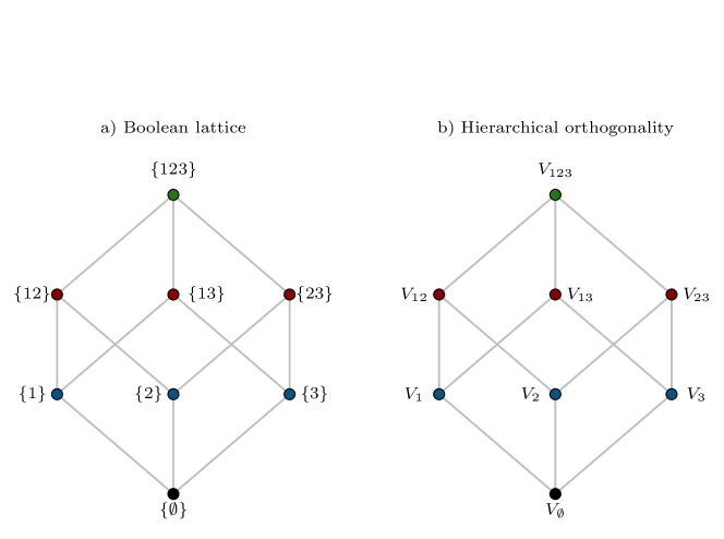
Figure 1: Illustration of the hierarchical orthogonality structure for three inputs. These Hasse diagrams are meant to be read from the bottom to the top. If an edge joins two elements, the bottom element is linked by the binary relation to the above element. On a), the binary relation is $\subset$, while on b) the binary relation is $\perp$.

In order to formally differentiate between the structurally hierarchical subspaces and those that are not necessarily orthogonal, we define two different sets. For any $A\in\mathcal{P}_{D}$, we first define the set of comparables (i.e., the elements of $\mathcal{P}_{D}$ that are subsets of $A$ or such that $A$ is a subset of), denoted

$$\mathcal{C}_{A}=\mathcal{P}_{A}\cup\left\{B\in\mathcal{P}_{D}:A\subseteq D\right\},$$

and notice that, for any $B\in\mathcal{C}_{A}$, $V_{B}\perp V_{A}$. Then, we define the set of uncomparables of $A$ as

$$\mathcal{U}_{A}=\mathcal{P}_{D}\setminus\mathcal{C}_{A},$$

and notice that, in general, for every $B\in\mathcal{U}_{A}$, $V_{A}$ is not necessarily orthogonal to $V_{B}$. And notice additionally that, for any $A\in\mathcal{P}_{D}$

$$\mathcal{P}_{D}=\mathcal{C}_{A}\cup\mathcal{U}_{A}.$$

This hierarchical orthogonality structure is intimately linked with the notion of projections, particularly the orthogonal and oblique projections onto the subspaces $V_{A}$.

3.3.2 Projections and their properties

First, assuming that Theorem 5 hold, we define several projectors onto the subspaces $V_{A}$, for every $A\in\mathcal{P}_{D}$. Let $A$ be any element of $\mathcal{P}_{D}$. Denote by $P_{A}$ the orthogonal projector onto $V_{A}$, i.e., ,

$$P_{A}:\mathbb{L}^{2}\left(\sigma_{X}\right)\rightarrow\mathbb{L}^{2}\left(\sigma_{X}\right),\quad\text{ such that }\textrm{Ran}\left(P_{A}\right)=V_{A}\text{ and }\textrm{Ker}\left(P_{A}\right)=V_{A}^{\perp}.$$

Since $V_{A}$ is a closed subspace of $\mathbb{L}^{2}\left(\sigma_{X}\right)$, the orthogonal projector $P_{A}$ is well and uniquely defined. Next, for any $B\subset A$, we define the restriction of $P_{B}$ on $\mathbb{L}^{2}\left(\sigma_{A}\right)$, denoted

$$P_{B}^{A}:\mathbb{L}^{2}\left(\sigma_{A}\right)\rightarrow\mathbb{L}^{2}\left(\sigma_{A}\right),\quad\text{ such that }\textrm{Ran}\left(P_{A}\right)=V_{B}\text{ and }\textrm{Ker}\left(P_{A}\right)=V_{B}^{\perp_{A}}.$$

Again, $V_{B}$ being a closed subspace of $\mathbb{L}^{2}\left(\sigma_{A}\right)$, this projector is unique and well-defined. Additionally, for every $A\in\mathcal{P}_{D}$, denote the following subspaces of $\mathbb{L}^{2}\left(\sigma_{X}\right)$

$$W_{A}=\bigoplus_{B\in\mathcal{P}_{D}:B\neq A}V_{B},$$

and the operators

$$Q_{A}:\mathbb{L}^{2}\left(\sigma_{X}\right) \rightarrow\mathbb{L}^{2}\left(\sigma_{X}\right)$$

$$G(X)=\sum_{B\in\mathcal{P}_{D}}G_{B}(X_{B}) \mapsto G_{A}(X_{A})$$

and notice that $Q_{A}$ is the projector onto $V_{A}$ parallel to $W_{A}$, which is well-defined thanks to the direct-sum decomposition of Theorem 5 (see [44] Theorem 3.4).

Now, we define projectors onto the subspaces $\mathbb{L}^{2}\left(\sigma_{A}\right)$, for every $A\in\mathcal{P}_{D}$. First, the orthogonal projector onto $\mathbb{L}^{2}\left(\sigma_{A}\right)$ is defined as

$$\mathbb{E}_{A}:\mathbb{L}^{2}\left(\sigma_{X}\right)\rightarrow\mathbb{L}^{2}\left(\sigma_{X}\right),\quad\text{ such that }\textrm{Ran}\left(\mathbb{E}_{A}\right)=\mathbb{L}^{2}\left(\sigma_{A}\right)\text{ and }\textrm{Ker}\left(P_{A}\right)=\mathbb{L}^{2}\left(\sigma_{A}\right)^{\perp},$$

and notice that, for any $H(X)\in\mathbb{L}^{2}\left(\sigma_{X}\right)$, $\mathbb{E}_{A}\left(H(X)\right)=\mathbb{E}\left[H(X)\mid\sigma_{A}\right]$, i.e., , it is in fact the conditional expectation of $H(X)$ given $X_{A}$ (see [31], Chapter 8). Additionally, denote the subspace

$$\overline{W}_{A}=\bigoplus_{B\in\mathcal{P}_{D},B\not\in\mathcal{P}_{A}}V_{B}$$

and the operator

$$\mathbb{M}_{A}:\mathbb{L}^{2}\left(\sigma_{X}\right) \rightarrow\mathbb{L}^{2}\left(\sigma_{X}\right)$$

$$G(X)=\sum_{B\in\mathcal{P}_{D}}G_{B}(X_{B}) \mapsto\sum_{B\in\mathcal{P}_{A}}G_{B}(X_{B})$$

and, thanks to Theorem 5, notice that $\mathbb{M}_{A}$ is the projection onto $\textrm{Ran}\left(\mathbb{M}_{A}\right)=\mathbb{L}^{2}\left(\sigma_{A}\right)$ parallel to $\textrm{Ker}\left(\mathbb{M}_{A}\right)=\overline{W}_{A}$.

The first observation is a particular consequence of the orthogonality structure, namely, the annihilating property (see, e.g., [28] Lemma 1, or [34]), which has been well-documented in the case of mutually independent inputs. This property admits a rather surprising generalization in the framework of Theorem 5.

Proposition 4 (Annihilating property).

We place ourselves in the framework of Theorem 5 and Corollary 1. For any $A\in\mathcal{P}_{D}$ and any $B\subset A$

$$P_{B}\left(Q_{A}\left(G(X)\right)\right)=P_{B}\left(G_{A}(X_{A})\right)=0.$$

Proof of Proposition 4.

From Proposition 3, for every $B\subset A$, one has that $V_{B}\perp V_{A}$, and thus $G_{A}(X_{A})\in V_{A}\subset V_{B}^{\perp}$. ∎

Another interesting result is the fact that the oblique projections $\left(Q_{A}\right)_{A\in\mathcal{P}_{D}}$ onto the $V_{A}$ can be expressed in terms of the oblique projections $\left(\mathbb{M}_{A}\right)_{A\in\mathcal{P}_{D}}$ onto the generated Lebesgue spaces.

Proposition 5 (Formula for oblique projections).

We place ourselves in the framework of Theorem 5 and Corollary 1. One has that, for any $G(X)\in\mathbb{L}^{2}\left(\sigma_{X}\right)$, and for any $A\in\mathcal{P}_{D}$

$$Q_{A}(G(X))=\sum_{B\in\mathcal{P}_{A}}(-1)^{|A|-|B|}\mathbb{M}_{A}(G(X)),$$

where $|.|$ denotes the cardinality of sets.

Proof of Proposition 5.

By definition of $\mathbb{M}_{A}$, one has that

$$\forall A\in\mathcal{P}_{D},\quad\mathbb{M}_{A}(G(X))=\sum_{B\in\mathcal{P}_{A}}Q_{A}(G(X)),$$

which, thanks to Rota’s generalization of the Möbius inversion formula for power-set valued functions [48, 33, 29], is equivalent to

$$\forall A\in\mathcal{P}_{D},\quad Q_{A}(G(X))=\sum_{B\in\mathcal{P}_{A}}(-1)^{|A|-|B|}\mathbb{M}_{A}(G(X)).$$

∎

In order to better visualize how the decomposition of Theorem 5 can be understood in terms of projections, one can take an example with two inputs $X_{1}$ and $X_{2}$, and a centered random output $G(X_{1},X_{2})\in\mathbb{L}^{2}\left(\sigma_{12}\right)$. Figure 2 illustrates this situation. $G(X_{1},X_{2})$ can be written as a sum of three elements, $G_{1}(X_{1})\in V_{1}$, $G_{2}(X_{2})\in V_{2}$ and $G_{12}(X_{1},X_{2})\in V_{12}$. $G_{12}(X_{1},X_{2})$ is none other than the orthogonal projection of $G$ onto $V_{12}$, due to the fact that $V_{12}$ is the orthogonal complement of $V_{1}+V_{2}$ and, naturally, $G_{1}(X_{1})+G_{2}(X_{2})=\left[I-P_{12}\right]\left(G(X)\right)$. Now, recall that since $V_{1}$ and $V_{2}$ are not necessarily orthogonal (which is represented as the angle $\alpha$ (which is non-zero, thanks to the Assumptions 1 and 2) in Figure 2), $G_{1}(X_{1})$ (resp. $G_{2}(X_{2})$) is none other than the oblique projection of $G(X)$ onto $V_{1}$ parallel to $V_{2}$ (resp. onto $V_{2}$ parallel to $V_{1}$).

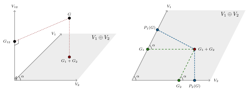
Figure 2: Illustration of a centered function decomposition with two dependent inputs.

3.4 Mutual independence

It is well-known that the independence of two $\sigma$-algebras is defined in terms of the orthogonality of the Lebesgue spaces they generate. More precisely, two sub $\sigma$-algebras $\mathcal{A}_{1}$ and $\mathcal{A}_{2}$ of a probability space $(\Omega,\mathcal{F},\mathbb{P})$ are said to be independent if $\mathbb{L}^{2}\left(\mathcal{A}_{1}\right)$ and $\mathbb{L}^{2}\left(\mathcal{A}_{2}\right)$ are orthogonal on the constant functions (see [39], Definition 3.0.1). More precisely,

$$\mathcal{A}_{1}\perp\!\!\!\perp\mathcal{A}_{2}\iff\mathbb{L}^{2}\left(\mathcal{A}_{1}\right)\cap\left[\mathbb{L}^{2}\left(\sigma_{\emptyset}\right)\right]^{\perp}\perp\mathbb{L}^{2}\left(\mathcal{A}_{2}\right)\cap\left[\mathbb{L}^{2}\left(\sigma_{\emptyset}\right)\right]^{\perp},$$

where $\perp$ is defined relative to $\mathbb{L}^{2}\left(\mathcal{F}\right)$. Additionally, two random elements $X,Y$ defined on $(\Omega,\mathcal{F},\mathbb{P})$ are considered independent if their generated $\sigma$-algebras are independent.

When dealing with a vector of random elements $X=(X_{1},\dots,X_{d})$, mutual independence is defined w.r.t. the independence of the generated $\sigma$-algebras. More precisely, $X$ is said to be mutually independent if

$$\forall A\in\mathcal{P}_{D},\quad\sigma_{A}\perp\!\!\!\perp\sigma_{D\setminus A}\iff c\left(\mathbb{L}^{2}\left(\sigma_{A}\right),\mathbb{L}^{2}\left(\sigma_{D\setminus A}\right)\right)=0.$$

Proposition 6.

Let $X$ be a vector of random elements. If $X$ is mutually independent, then Assumption 1 hold.

Proof of Proposition 6.

From [39], note that for two $\sigma$-algebras $\mathcal{A}_{1}$ and $\mathcal{A}_{2}$,

$$\mathcal{A}_{1}\perp\!\!\!\perp\mathcal{A}_{2}\quad\implies\quad\mathcal{A}_{1}\cap\mathcal{A}_{2}=\sigma_{\emptyset}.$$

Suppose that Assumption 1 does not hold. Hence, in particular, for any $A\in\mathcal{P}_{D}$,

$$\sigma_{A}\cap\sigma_{D\setminus A}\neq\sigma_{\emptyset}.$$

It implies that $\sigma_{A}$ and $\sigma_{D\setminus A}$ cannot be independent. Hence, since this holds for any $A\in\mathcal{P}_{D}$, $X$ cannot be mutually independent. The result is proven by taking the converse implication. ∎

Proposition 7.

Let $X$ be a vector of random elements. $X$ is mutually independent if and only if $\forall A,B\in\mathcal{P}_{D}$, $A\neq B$,

$$c\left(\mathbb{L}^{2}\left(\sigma_{A}\right),\mathbb{L}^{2}\left(\sigma_{B}\right)\right)=0.$$

Proof of Proposition 7.

Notice that, in the general case, if $B\subset A$, then $c\left(\mathbb{L}^{2}\left(\sigma_{A}\right),\mathbb{L}^{2}\left(\sigma_{B}\right)\right)$ is necessarily equal to zero. Thus, we focus on the case where $A\cap B=C\not\in\{A,B\}$.

Now, suppose that for any $A,B\in\mathcal{P}_{D}$, $c\left(\mathbb{L}^{2}\left(\sigma_{A}\right),\mathbb{L}^{2}\left(\sigma_{B}\right)\right)=0$. Hence, in particular, if for every $A\in\mathcal{P}_{D}$

$$c\left(\mathbb{L}^{2}\left(\sigma_{A}\right),\mathbb{L}^{2}\left(\sigma_{D\setminus A}\right)\right)=0\iff\sigma_{A}\perp\!\!\!\perp\sigma_{D\setminus A}$$

which is equivalent to $X$ being mutually independent.

Suppose that $X$ is mutually independent, and thus, $P_{X}=\bigtimes_{i\in D}P_{X_{i}}$, which implies that, for any $A,B\in\mathcal{P}_{D}$, with $A\cap B=C\not\in\{A,B\}$,

$$\mathbb{E}_{A}\circ\mathbb{E}_{B}=\mathbb{E}_{B}\circ\mathbb{E}_{A}=\mathbb{E}_{C},$$

Thus, the orthogonal projections onto $\mathbb{L}^{2}\left(\sigma_{A}\right)$ and $\mathbb{L}^{2}\left(\sigma_{B}\right)$ commute, which is equivalent to (see (2))

$$c\left(\mathbb{L}^{2}\left(\sigma_{A}\right),\mathbb{L}^{2}\left(\sigma_{B}\right)\right)=0.$$

∎

Corollary 2.

Let $X$ be a vector of random elements. $X$ is mutually independent if and only if its maximal coalitional precision matrix $\Delta$ is the identity.

Proof of Proposition 2.

It is a direct consequence of Proposition 7, by definition of $\Delta$. ∎

Hence, if the inputs are mutually independent, both Assumption 1 and Assumption 2 hold and lead to the very particular case of $\Delta$ being the identity matrix. When it comes to the resulting decomposition of $\mathbb{L}^{2}\left(\sigma_{X}\right)$, one has the following result:

Proposition 8.

We place ourselves in the framework of Theorem 5. $X$ is mutually independent if and only if

$$\forall A,B\in\mathcal{P}_{D},B\neq A\quad V_{A}\perp V_{B}.$$

Proof of Proposition 8.

Notice that, in general, if Assumption 1 hold, one has that for any $A,B\in\mathcal{P}_{D}$, $B\neq A$

$$c_{0}\left(V_{A},V_{B}\right)\leq c\left(\mathbb{L}^{2}\left(\sigma_{A}\right),\mathbb{L}^{2}\left(\sigma_{B}\right)\right).$$

Note that, from Proposition 6, Assumption 1 holds for a mutually independent $X$. Moreover, notice from Proposition 7 that $X$ is mutually independent if and only if, $\forall A,B\in\mathcal{P}_{D}$, $A\neq B$, $c\left(\mathbb{L}^{2}\left(\sigma_{A}\right),\mathbb{L}^{2}\left(\sigma_{B}\right)\right)=0$, thus necessarily $c_{0}\left(V_{A},V_{B}\right)=0$, which is equivalent to $V_{A}\perp V_{B}$. ∎

Proposition 8 is, in fact, equivalent to the Hoeffding functional decomposition for mutually independent inputs [27, 10], which can be seen as a very particular case of Theorem 5 where $X$ admits a maximal coalitional precision matrix equal to the identity.

4 Interpretable decomposition of quantities of interest

4.1 Canonical evaluation decomposition

For $\omega\in\Omega$, denote $x=X(\omega)\in E$ an observation of $X$. Subsequently, denote $G(x)\in\mathbb{R}$ the evaluation on $x$ of a random output $G(X)\in\mathbb{L}^{2}\left(\sigma_{X}\right)$. In the XAI literature, “explanation” methods aim at decomposing $G(x)$ into parts for which each input is responsible [1]. They often rely on cooperative game theory, particularly on the Shapley values [51], an allocation with seemingly reasonable properties [38]. However, allocations can be understood as aggregations of coalitional decompositions [29], which can be trivially chosen. However, Theorem 5, and in particular Corollary 1 offers a canonical coalitional decomposition of an evaluation of a random output $G(X)\in\mathbb{L}^{2}\left(\sigma_{X}\right)$.

Definition 4 (Canonical decomposition of an evaluation).

Let $X=(X_{1},\dots,X_{d})$ be a vector of random elements, let $G(X)$ be in $\mathbb{L}^{2}\left(\sigma_{X}\right)$ and assume that Assumptions 1 and 2 hold. For any $\omega\in\Omega$, denote $x=X(\omega)$. The canonical coalitional decomposition of the evaluation $G(x)$ is defined as

$$G(x)=\sum_{A\in\mathcal{P}_{D}}G_{A}(x_{A}),$$

where $x_{A}=X_{A}(\omega)$, and

$$G_{A}(x_{A})=Q_{A}\left(G(x)\right)=\sum_{B\in\mathcal{P}_{A}}(-1)^{|A|-|B|}\mathbb{M}_{B}\left(G(x)\right),$$

where $Q_{A}$ is the projection onto $V_{A}$ parallel to $W_{A}$ and $\mathbb{M}_{A}$ is the projection onto $\mathbb{L}^{2}\left(\sigma_{A}\right)$ parallel to $\overline{W}_{A}$.

The usual coalitional decomposition of choice, even for dependent inputs, relies on choosing conditional expectations (also known as “conditional Shapley values”) [38]. However, the following results show that this choice entails a canonical decomposition if and only if the inputs are mutually independent.

Proposition 9.

Let $X=(X_{1},\dots,X_{d})$ be a vector of random elements, let $G(X)$ be in $\mathbb{L}^{2}\left(\sigma_{X}\right)$, and assume that Assumptions 1 and 2 hold. Then,

$$G_{A}(x_{A})=\sum_{B\in\mathcal{P}_{A}}(-1)^{|A|-|B|}\mathbb{E}_{B}\left(G(x)\right),\quad\forall A\in\mathcal{P}_{D}$$

if and only if $X$ is mutually independent.

Proof of Proposition 9.

First, notice that $\mathbb{M}_{A}=\mathbb{E}_{A}$ if and only if $\overline{W}_{A}$ is the orthogonal complement of $\mathbb{L}^{2}\left(\sigma_{A}\right)$. One can notice that, $\overline{W}_{A}$ is a complement of $\mathbb{L}^{2}\left(\sigma_{A}\right)$ in $\mathbb{L}^{2}\left(\sigma_{X}\right)$, and from Proposition 8, one has that

$$\mathbb{L}^{2}\left(\sigma_{A}\right)=\bigoplus_{B\in\mathcal{P}_{A}}V_{B}\perp\overline{W}_{A}=\bigoplus_{B\in\mathcal{P}_{D},B\not\in\mathcal{P}_{A}}V_{B},$$

hold for every $A\in\mathcal{P}_{D}$ if and only if $X$ is mutually independent. In this case, $\overline{W}_{A}$ is an orthogonal complement of $\mathbb{L}^{2}\left(\sigma_{A}\right)$, and by unicity, $\overline{W}_{A}=\mathbb{L}^{2}\left(\sigma_{A}\right)^{\perp}$, and thus $\mathbb{M}_{A}=\mathbb{E}_{A}$. ∎

Hence, the choice of conditional expectations for the coalitional decomposition to be canonical is equivalent to $X$ being mutually independent. A large set of allocations can be seen as aggregations of a coalitional decomposition. In particular, one can define the canonical Shapley attribution scheme by using the representation of the Shapley values due to Harsanyi [25, 55].

Definition 5 (Canonical Shapley attribution).

Let $X=(X_{1},\dots,X_{d})$ be a vector of random elements, suppose that Assumptions 1 and 2 hold, and let $G(X)\in\mathbb{L}^{2}\left(\sigma_{X}\right)$. The canonical Shapley attribution of an evaluation $G(x)$ is the vector $\textrm{C-Sh}=\left(\textrm{C-Sh}_{1},\dots\textrm{C-Sh}_{d}\right)\in\mathbb{R}^{d}$ given by

$$\textrm{C-Sh}_{i}=\sum_{A\in\mathcal{P}_{D}:i\in A}\frac{Q_{A}(G(x))}{|A|}=\sum_{A\in\mathcal{P}_{D}:i\in A}\frac{\sum_{B\in\mathcal{P}_{A}}(-1)^{|A|-|B|}\mathbb{M}_{A}\left[G(x)\right]}{|A|}.$$

Additionally, one has that

$$\sum_{i=1}^{d}\textrm{C-Sh}_{i}=G(x).$$

Hence, the canonical Shapley attribution are the Shapley values of the cooperative game $(D,v)$ where the value function $v$ is given by

$$v(A)=\mathbb{M}_{A}\left[G(X)\right]=\sum_{B\in\mathcal{P}_{A}}Q_{A}(G(X)),\quad\forall A\in\mathcal{P}_{D},$$

and the subsequent Harsanyi dividends [25, 55, 15] of $(D,v)$ are given by

$$\mathcal{D}_{v}(A)=Q_{A}(G(X))=\sum_{B\in\mathcal{P}_{A}}(-1)^{|A|-|B|}\mathbb{M}_{A}\left[G(x)\right],\quad\forall A\in\mathcal{P}_{D}.$$

While these indices rely on the natural decomposition of $\mathbb{L}^{2}\left(\sigma_{X}\right)$ in the context of dependent inputs, they remain an aggregation of the canonical decomposition of $G(X)$. They can be interpreted as an egalitarian redistribution of the canonical interaction evaluations among the $d$ inputs. However, as all aggregations do, they bear less information about $G(X)$ than the canonical decomposition itself.

4.2 Variance decomposition

Performing a variance decomposition of a black-box model is paramount in quantifying a set of inputs’ influence (or importance) towards a multivariate model [10]. Let $G(X)$ be a random output and denote its variance

$$\mathbb{V}\left(G(X)\right)=\mathbb{E}\left[\left(G(X)-\mathbb{E}\left[G(X)\right]\right)^{2}\right]=\mathbb{E}\left[G(X)^{2}\right]-\mathbb{E}\left[G(X)\right]^{2}.$$

Suppose $G(X)$ describes a complex system. In that case, its variance can be interpreted as the “amount” of uncertainty due to the probabilistic nature of the inputs [14], which is at the cornerstone of uncertainty propagation and sensitivity analysis.

We propose two ways to approach the problem of decomposing $\mathbb{V}\left(G(X)\right)$. The canonical variance decomposition relies on the canonical decomposition of $G(X)$ (see Corollary 1). In contrast, the organic variance decomposition aims at defining and disentangling pure interaction effects from dependence effects.

4.2.1 Canonical variance decomposition

In light of Corollary 1, the canonical variance decomposition of $G(X)$ is rather intuitive. It relies on the following rationale:

$$\mathbb{V}\left(G(X)\right) =\textrm{Cov}\left(G(X),G(X)\right)$$

$$=\sum_{A\in\mathcal{P}_{D}}\textrm{Cov}\left(G_{A}(X_{A}),G(X)\right)$$

$$=\sum_{A\in\mathcal{P}_{D}}\left[\mathbb{V}\left(G_{A}(X_{A})\right)+\sum_{B\in\mathcal{U}_{A}}\textrm{Cov}\left(G_{A}(X_{A}),G_{B}(X_{B})\right)\right].$$

reminiscent of the “covariance decomposition” [54, 7, 26, 10]. Two indices arise from this decomposition.

Definition 6 (Canonical variance decomposition).

We place ourselves in the framework of Theorem 5. For any $A\in\mathcal{P}_{D}$, let

$$S_{A}^{U}=\mathbb{V}\left(G_{A}(X_{A})\right),$$

defines the structural contribution of $X_{A}$ to $G(X)$, while

$$S_{A}^{C}=\sum_{B\in\mathcal{U}_{A}}\textrm{Cov}\left(G_{A}(X_{A}),G_{B}(X_{B})\right),$$

represents the correlative contribution of $X_{A}$ to $G(X)$.

Remark 4.

It is important to note that both the magnitude of $S_{A}^{U}$ and $S_{A}^{C}$ varies w.r.t. the dependence structure of the inputs (i.e., the angles between the subspaces $\left(V_{A}\right)_{A\in\mathcal{P}_{D}}$). It is illustrated in Section 5. Hence, $S_{A}^{C}$ cannot be understood as a pure quantification of “dependence effects” and $S_{A}^{U}$ cannot quantify possibly quantify “pure interaction”.

The canonical decomposition of $\mathbb{V}\left(G(X)\right)$ is suitable in practice if the dependence structure of $X$ is assumed to be inherent in the modeling of the studied phenomenon. In other words, if one aims to understand the global relationship between $X$ and $G(X)$.

Proposition 10.

We place ourselves in the framework of Theorem 5. Then, for any $A\in\mathcal{P}_{D}$

$$S_{A}^{C}=\sum_{B\in\mathcal{P}_{A}}(-1)^{|A|-|B|}\textrm{Cov}\left(\mathbb{M}_{B}(G(X)),\left[I-\mathbb{M}_{A}\right](G(X))\right).$$

Proof of Proposition 10.

First, recall that, for any $A\in\mathcal{P}_{D}$,

$$G_{A}(X_{A})=\sum_{B\in\mathcal{P}_{A}}(-1)^{|A|-|B|}\mathbb{M}_{B}(G(X)),$$

and hence,

$$\sum_{B\in\mathcal{P}_{A}}(-1)^{|A|-|B|}\textrm{Cov}\left(\mathbb{M}_{B}(G(X)),\left[I-\mathbb{M}_{A}\right](G(X))\right) =\textrm{Cov}\left(G_{A}(X_{A}),\left[I-\mathbb{M}_{A}\right](G(X))\right)$$

$$=\sum_{B\in\mathcal{P}_{D}:B\not\in\mathcal{P}_{A}}\textrm{Cov}\left(G_{A}(X_{A}),G_{B}(X_{B})\right).$$

However, notice that $\mathcal{U}_{A}\subset\mathcal{P}_{D}\setminus\mathcal{P}_{A}$, and that, for any $B\in\mathcal{P}_{D}\setminus\mathcal{P}_{A}$ with $B\not\in\mathcal{U}_{A}$,

$$\textrm{Cov}\left(G_{A}(X_{A}),G_{B}(X_{B})\right)=0,$$

and hence,

$$\sum_{B\in\mathcal{P}_{A}}(-1)^{|A|-|B|}\textrm{Cov}\left(\mathbb{M}_{B}(G(X)),\left[I-\mathbb{M}_{A}\right](G(X))\right) =\sum_{B\in\mathcal{P}_{D}:B\not\in\mathcal{P}_{A}}\textrm{Cov}\left(G_{A}(X_{A}),G_{B}(X_{B})\right)$$

$$=\sum_{B\in\mathcal{U}_{A}}\textrm{Cov}\left(G_{A}(X_{A}),G_{B}(X_{B})\right)$$

$$=S_{A}^{C}.$$

∎

Proposition 11.

We place ourselves in the framework of Theorem 5. Then, for any $A\in\mathcal{P}_{D}$

$$S_{A}^{U}=\sum_{B\in\mathcal{P}_{A}}(-1)^{|A|-|B|}\left[\mathbb{V}\left(\mathbb{M}_{B}(G(X))\right)-\textrm{Cov}\left(\mathbb{M}_{B}(G(X)),\left[I-\mathbb{M}_{A}\right](G(X))\right)\right].$$

Proof of Proposition 11.

First, recall that

$$\mathbb{M}_{A}(G(X))=\sum_{B\in\mathcal{P}_{A}}G_{B}(X_{B}).$$

Thus,

$$\mathbb{V}\left(\mathbb{M}_{A}(G(X))\right) =\mathbb{V}\left(\sum_{B\in\mathcal{P}_{A}}G_{B}(X_{B})\right)$$

$$=\sum_{B\in\mathcal{P}_{A}}\mathbb{V}\left(G_{B}(X_{B})\right)+\sum_{C\in\mathcal{U}_{A}}\textrm{Cov}\left(G_{B}(X_{B}),G_{C}(X_{C})\right)$$

$$=\sum_{B\in\mathcal{P}_{A}}S_{B}^{U}+S_{B}^{C}$$

which is equivalent to

$$\mathbb{V}\left(\mathbb{M}_{A}(G(X))\right)-\sum_{B\in\mathcal{P}_{A}}S_{B}^{C}=\sum_{B\in\mathcal{P}_{A}}S_{B}^{U}.$$

However, notice that, $\forall A\in\mathcal{P}_{D}$

$$\sum_{B\in\mathcal{P}_{A}}S_{B}^{C}=\textrm{Cov}\left(\mathbb{M}_{A}(G(X)),\left[I-\mathbb{M}_{A}\right](G(X))\right),$$

and thus, $\forall A\in\mathcal{P}_{D}$

$$\mathbb{V}\left(\mathbb{M}_{A}(G(X))\right)-\textrm{Cov}\left(\mathbb{M}_{A}(G(X)),\left[I-\mathbb{M}_{A}\right](G(X))\right)=\sum_{B\in\mathcal{P}_{D}}S_{B}^{U}.$$

Using Rota’s generalization of the Möbius inversion formula applied to the power-set, it yields that $\forall A\in\mathcal{P}_{D}$

$$S_{A}^{U}=\sum_{B\in\mathcal{P}_{A}}(-1)^{|A|-|B|}\left[\mathbb{V}\left(\mathbb{M}_{B}(G(X))\right)-\textrm{Cov}\left(\mathbb{M}_{B}(G(X)),\left[I-\mathbb{M}_{A}\right](G(X))\right)\right].$$

∎

4.2.2 Organic variance decomposition

The goal of the organic variance decomposition is to separate “pure interaction effects” to “dependence effects”. Pure interaction can be seen as the study of the functional relation between the inputs $X$ and the random output $G(X)$ without considering the dependence structure of $X$. Hence, it amounts to performing a canonical variance decomposition of $\mathbb{V}\left(G(X)\right)$ under mutual independence of $X$. Formally, let $X=(X_{1},\dots,X_{d})$ be a vector of random elements. The induced probability measure $P_{X}$ is not necessarily the product measure $\bigtimes_{i\in D}P_{X_{i}}$. Now, denote $\widetilde{X}=(\widetilde{X}_{1},\dots,\widetilde{X}_{d})$ the vector of random elements such that

$$\widetilde{X}_{i}=X_{i}\text{ a.s.}\quad\text{ and }\quad P_{\widetilde{X}}:=\bigtimes_{i\in D}P_{X_{i}}.$$

In other words, $X$ and $\widetilde{X}$ have the same univariate marginals, but $\widetilde{X}$ is the mutual independent version of $X$ and, for any $A\in\mathcal{P}_{D}$, denote $\widetilde{X}_{A}$ its marginals. Suppose that $G(X)\in\mathbb{L}^{2}\left(\sigma_{X}\right)$ and $G(\widetilde{X})\in\mathbb{L}^{2}\left(\sigma_{\widetilde{X}}\right)$, and, for any $H(\widetilde{X})$ denote

$$\mathbb{E}^{\perp\!\!\!\perp}\left[H(\widetilde{X})\right]=\int_{E}H(x)\prod_{i\in D}dP_{X_{i}}(x_{i}),\quad\text{ and }\mathbb{V}^{\perp\!\!\!\perp}\left(H(X)\right)=\mathbb{E}^{\perp\!\!\!\perp}\left[\left(H(\widetilde{X})-\mathbb{E}^{\perp\!\!\!\perp}\left[H(\widetilde{X})\right]\right)^{2}\right].$$

Notice that, since $\widetilde{X}$ is mutually independent, it respects both Assumptions 1 and 2, and hence, one can perform the following canonical decomposition in $\mathbb{L}^{2}\left(\sigma_{\widetilde{X}}\right)$

$$G(\widetilde{X})=\sum_{A\in\mathcal{P}_{D}}\widetilde{G}_{A}(\widetilde{X}_{A}),$$

where the $\widetilde{G}_{A}(\widetilde{X}_{A})$ are all pairwise orthogonal (see Section 3.4), and hence

$$\mathbb{V}^{\perp\!\!\!\perp}\left(G(\widetilde{X})\right)=\sum_{A\in\mathcal{P}_{D}}\mathbb{V}^{\perp\!\!\!\perp}\left(\widetilde{G}_{A}(\widetilde{X}_{A})\right)$$

We propose the following indices.

Definition 7 (Pure interaction effect).

We place ourselves in the framework of Theorem 5. For any $A\in\mathcal{P}_{D}$, let

$$S_{A}=\frac{\mathbb{V}^{\perp\!\!\!\perp}\left(\widetilde{G}_{A}\right)}{\mathbb{V}^{\perp\!\!\!\perp}\left(G(\widetilde{X})\right)}\mathbb{V}\left(G(X)\right)$$

define the pure interaction indices.

These indices are, in fact, the Sobol’ indices of $G(\widetilde{X})$ [53], which are known in the literature as quantifying pure interaction [10]. These indices can also be expressed as functions of the orthogonal projections onto the subspaces $\mathbb{L}^{2}\left(\sigma_{\widetilde{X}_{A}}\right)$ as follows

$$S_{A}=\sum_{B\in\mathcal{P}_{A}}(-1)^{|A|-|B|}\mathbb{E}^{\perp\!\!\!\perp}_{B}\left(G(\widetilde{X})\right),$$

where, $\forall A\in\mathcal{P}_{D}$

$$\mathbb{E}^{\perp\!\!\!\perp}_{B}\left(G(\widetilde{X})\right)=\int_{E_{D\setminus A}}G(\widetilde{X}_{A},x_{D\setminus A})\prod_{i\in D\setminus A}dP_{X_{i}}(x_{i}).$$

For further considerations about these indices, we refer the interested reader to [10].

Remark 5.

In certain situations, when $X$ is from a certain family of random vectors, it is possible to find a mapping $T:E\rightarrow E$ such that

$$\widetilde{X}=T(X).$$

In particular, if $P_{X}$ is in the family of elliptical distribution, it amounts to performing a Nataf transform of the inputs [36, 37].

When defining dependence effects, one desirability criterion can be brought forward: the set of indices must all be equal to zero if and only if $X$ is mutually independent. Formally, denote $(\phi_{A})_{A\in\mathcal{P}_{D}}$ an abstract set of dependence effects. One must have that

$$\phi_{A}=0,\quad\forall A\in\mathcal{P}_{D}\quad\iff\quad X\text{ is mutually independent}.$$

Thanks to the geometric interpretation of the canonical decomposition of $\mathbb{L}^{2}\left(\sigma_{X}\right)$ (see , Section 3.3), many quantities can be defined that respect this property. However, we focus on one particular quantity, which can be easily interpreted.

Lemma 6.

We place ourselves in the framework of Theorem 5. Let $G(X)\in\mathbb{L}^{2}\left(\sigma_{X}\right)$. Then,

$$Q_{A}\left(G(X)\right)=P_{A}\left(G(X)\right)\text{ a.s.},\quad\forall A\in\mathcal{P}_{D}\quad\iff\quad X\text{ is mutually independent.}$$

Proof of Lemma 6.

First, suppose that $X$ is mutually independent. By Proposition 8, one has that

$$\forall A,B\in\mathcal{P}_{D},B\neq A\quad V_{A}\perp V_{B},$$

which entails that

$$V_{A}\perp W_{A}=\mathop{\mathchoice{\vbox{\hbox{\leavevmode\resizebox{}{9.00005pt}{\raisebox{0.0pt}{$\displaystyle+$}}}}\vphantom{\sum}}{\vbox{\hbox{\leavevmode\resizebox{}{9.00005pt}{\raisebox{0.0pt}{$\textstyle+$}}}}\vphantom{\sum}}{\vbox{\hbox{\leavevmode\resizebox{}{6.30003pt}{\raisebox{0.0pt}{$\scriptstyle+$}}}}\vphantom{\sum}}{\vbox{\hbox{\leavevmode\resizebox{}{4.50002pt}{\raisebox{0.0pt}{$\scriptscriptstyle+$}}}}\vphantom{\sum}}}\slimits@_{B\in\mathcal{P}_{D}:B\neq A}V_{B}.$$

However, notice that $W_{A}$ still complements $V_{A}$ in $\mathbb{L}^{2}\left(\sigma_{X}\right)$. Furthermore, by unicity of the orthogonal complement, one has that $W_{A}=V_{A}^{\perp}$. Thus,

$$\textrm{Ran}\left(Q_{A}\right)=V_{A},\quad\textrm{Ker}\left(Q_{A}\right)=V_{A}^{\perp},$$

and thus $Q_{A}=P_{A}$, leading to

$$Q_{A}\left(G(X)\right)=P_{A}\left(G(X)\right)\text{ a.s.}$$

Now, suppose that for any $A\in\mathcal{P}_{D}$, $Q_{A}\left(G(X)\right)=P_{A}\left(G(X)\right)$ a.s. Hence, it implies that

$$\forall A\in\mathcal{P}_{D},G_{A}(X_{A})=P_{A}\left(G(X)\right).$$

which implies that $P_{A}=Q_{A}$, since the above equation defines the operator $Q_{A}$. Thus, $P_{A}$ and $Q_{A}$ must share the same ranges and nullspaces. In particular,

$$\textrm{Ker}\left(Q_{A}\right)=\textrm{Ker}\left(P_{A}\right)=V_{A}^{\perp},$$

implying that $W_{A}=V_{A}^{\perp}$, which leads to

$$V_{A}\perp W_{A},\forall A\in\mathcal{P}_{D}\quad\iff\quad V_{A}\perp V_{B},\forall A,B\in\mathcal{P}_{D},B\neq A.$$

Finally, thanks to Proposition 8, notice that this is equivalent to $X$ being mutually independent. ∎

In other words, Lemma 6 states that the oblique projections $Q_{A}$ are orthogonal if and only if $X$ is mutually independent. Hence, a rather intuitive index would quantify the distance between these two projections.

Definition 8 (Dependence effects).

We place ourselves in the framework of Theorem 5. For any $A\in\mathcal{P}_{D}$, let

$$S_{A}^{D}=\mathbb{V}\left(Q_{A}(G(X))-P_{A}(G(X))\right)=\mathbb{E}\left[\left(Q_{A}(G(X))-P_{A}(G(X))\right)^{2}\right]$$

define the dependence effect of $X_{A}$.

Furthermore, these indices are naturally all zero if and only if $X$ is mutually independent.

Proposition 12.

$$S_{A}^{D}=0,\forall A\in\mathcal{P}_{D}\quad\iff\quad X\text{ is mutually independent.}$$

Proof of Proposition 12.

This is a direct consequence of Lemma 6, coupled with the fact that the expected squared distance is a distance. ∎

4.2.3 Links between the canonical and organic indices

It is possible to draw some links between the canonical and organic indices. The first one is that, in certain situations, the dependence effects can be written w.r.t. both the structural and correlative indices.

Proposition 13.

We place ourselves in the framework of Theorem 5. For every $A\in\mathcal{P}_{D}$, if $G_{A}(X_{A})\neq 0$, then

$$S_{A}^{D}=\frac{\left(S_{A}^{C}\right)^{2}}{S_{A}^{U}}.$$

Proof of Proposition 13.

Notice that, if $G_{A}(X_{A})\neq 0$, then it is always possible to write

$$P_{A}(G(X))=\frac{\mathbb{E}\left[G(X)G_{A}(X_{A})\right]}{\mathbb{E}\left[G_{A}(X_{A})^{2}\right]}G_{A}(X_{A}).$$

However, notice that

$$\mathbb{E}\left[G(X)G_{A}(X_{A})\right] =\mathbb{E}\left[G_{A}(X_{A})^{2}\right]+\sum_{B\in\mathcal{U}_{A}}\mathbb{E}\left[G_{A}(X_{A})G_{B}(X_{B})\right]$$

$$=\mathbb{V}\left(G_{A}(X_{A})\right)+\sum_{B\in\mathcal{U}_{A}}\textrm{Cov}\left(G_{A},G_{B}\right)$$

$$=S_{A}^{U}+S_{A}^{C}$$

since the summands are centered. Thus,

$$P_{A}(G(X))=\frac{S_{A}^{U}+S_{A}^{C}}{S_{A}^{U}}G_{A}(X_{A})=\left(1+\frac{S_{A}^{C}}{S_{A}^{U}}\right)G_{A}(X_{A})$$

and thus,

$$G_{A}(X_{A})-P_{A}(G(X))=\frac{S_{A}^{C}}{S_{A}^{U}}G_{A}(X_{A}),$$

and thus

$$\mathbb{V}\left(G_{A}(X_{A})-P_{A}(G(X))\right) =\mathbb{E}\left[\left(G_{A}(X_{A})-P_{A}(G(X))\right)^{2}\right]$$

$$=\mathbb{E}\left[\left(G_{A}(X_{A})\frac{S_{A}^{C}}{S_{A}^{U}}\right)^{2}\right]$$

$$=\left(\frac{S_{A}^{C}}{S_{A}^{U}}\right)^{2}\mathbb{E}\left[G_{A}(X_{A})^{2}\right]$$

$$=\frac{\left(S_{A}^{C}\right)^{2}}{S_{A}^{U}}$$

∎

The second link entails that the correlative effects sum up to the sum of the differences between the structural and pure interaction effects.

Proposition 14.

We place ourselves in the framework of Theorem 5. One has that

$$\sum_{A\in\mathcal{P}_{D}}S_{A}^{C}=\sum_{A\in\mathcal{P}_{D}}\left[S_{A}-S_{A}^{U}\right].$$

Proof of Proposition 14.

Notice that

$$\sum_{A\in\mathcal{P}_{D}}S_{A}=\mathbb{V}\left(G(X)\right)=\sum_{A\in\mathcal{P}_{D}}S_{A}^{U}+S_{A}^{C}$$

and thus

$$\sum_{A\in\mathcal{P}_{D}}\left[S_{A}-S_{A}^{U}\right]=\sum_{A\in\mathcal{P}_{D}}S_{A}^{C}.$$

∎

5 Illustration: two Bernoulli inputs

In order to illustrate Theorem 5, one can take an interest in a very particular case: $X$ is comprised of two Bernoulli random variables (here, $E=\{0,1\}^{2}$) $X_{1}$ and $X_{2}$, with success probability $q_{1}$ and $q_{2}$ respectively. The joint law of $X$ can be fully expressed using three free parameters: $q_{1}$, $q_{2}$, and $\rho=\mathbb{E}\left[X_{1}X_{2}\right]$. More precisely, one has that:

$$\begin{cases}p_{00}=1-q_{1}-q_{2}+\rho\\ p_{01}=q_{2}-\rho\\ p_{10}=q_{1}-\rho\\ p_{11}=\rho\end{cases}$$

where, for $i,j\in\{0,1\}$, one denotes $p_{ij}=\mathbb{P}\left(\left\{X_{1}=i\right\}\cap\left\{X_{2}=j\right\}\right)$. Denote the $(4\times 4)$ diagonal matrix $P=\textrm{diag}(p_{00},p_{01},p_{10},p_{11})$. Any function $G:\{0,1\}^{2}\rightarrow\mathbb{R}$ can be represented as a vector in $\mathbb{R}^{4}$, where each element represents a value that $G$ can take w.r.t. the values taken by $X$. For $i,j\in\{0,1\}$, denote $G_{ij}=G(i,j)$, and thus

$$G=\begin{pmatrix}G_{00}\\ G_{01}\\ G_{10}\\ G_{11}\end{pmatrix},$$

where each $G_{ij}$ can be observed with probability $p_{ij}$.

5.1 Canonical decomposition as solving equations

In this particular case, one can analytically compute the decomposition of $G$ related to Theorem 5. It can be performed by finding suitable unit-norm vectors in $\mathbb{R}^{4}$

$$v_{\emptyset}=\begin{pmatrix}c\\ c\\ c\\ c\end{pmatrix},v_{1}=\begin{pmatrix}g_{0}\\ g_{0}\\ g_{1}\\ g_{1}\end{pmatrix},v_{2}=\begin{pmatrix}h_{0}\\ h_{1}\\ h_{0}\\ h_{1}\end{pmatrix},v_{12}=\begin{pmatrix}k_{00}\\ k_{01}\\ k_{10}\\ k_{11}\end{pmatrix}$$

such that

$$\begin{cases}v_{\emptyset}^{\top}Pv_{1}=0\\ v_{\emptyset}^{\top}Pv_{2}=0\\ v_{\emptyset}^{\top}Pv_{12}=0\\ v_{12}^{\top}Pv_{1}=0\\ v_{12}^{\top}Pv_{2}=0\\ \end{cases},\quad\text{ and },\quad\begin{cases}v_{\emptyset}^{\top}Pv_{\emptyset}=1\\ v_{1}^{\top}Pv_{1}=1\\ v_{2}^{\top}Pv_{2}=1\\ v_{12}^{\top}Pv_{12}=1\\ \end{cases}$$ (4)

which results in a system of nine equations with nine real unknown parameters (i.e., $c$ for $v_{\emptyset}$, $h_{0},h_{1}$ for $v_{1}$, $g_{0},g_{1}$ for $v_{2}$, and $k_{00},k_{01},k_{10},k_{11}$ for $v_{12}$). Given these vectors, one has that any function $G$ can be written as

$$G=ev_{\emptyset}+\alpha v_{1}+\beta v_{2}+\delta v_{12},$$

resulting in four additional equations with four unknown parameters. These 13 equations and 13 parameters can be found analytically.

In our case, we used the symbolic programming package sympy to perform these calculations [41]. We refer the interested reader to the accompanying GitHub repository for the analytical formulas obtained for this decomposition, as well as the analytical formulas of the indices introduced in Section 4. The remainder of this section is dedicated to discussing one interesting finding.

5.2 Angle, comonotonicity and definite positiveness of $\Delta$

First, notice the following equality, which holds in general.

Proposition 15.

We place ourselves in the framework of Theorem 5. Let $i,j\in D$ such that $i\neq j$. Then,

$$c\left(\mathbb{L}^{2}\left(\sigma_{i}\right),\mathbb{L}^{2}\left(\sigma_{j}\right)\right)=c_{0}\left(V_{i},V_{j}\right)$$

Proof of Proposition 15.

First, notice that under Assumption 1, one has that, for every $i,j\in D$, $i\neq j$

$$c_{0}\left(V_{i},V_{j}\right)\leq c\left(\mathbb{L}^{2}\left(\sigma_{i}\right),\mathbb{L}^{2}\left(\sigma_{j}\right)\right).$$

Next, recall the following classical inclusion result. Let $M,N,K$ be subspaces of a Hilbert space $\mathcal{H}$. Then,

$$\left(M\cap K\right)+\left(N\cap K\right)\subset\left(M+N\right)\cap K.$$

And hence, one has that

$$c\left(\mathbb{L}^{2}\left(\sigma_{i}\right),\mathbb{L}^{2}\left(\sigma_{j}\right)\right) =c_{0}\left(\mathbb{L}^{2}\left(\sigma_{i}\right)\cap V_{\emptyset}^{\perp},\mathbb{L}^{2}\left(\sigma_{j}\right)\cap V_{\emptyset}^{\perp}\right)$$

$$=c_{0}\left(\left(V_{\emptyset}+V_{i}\right)\cap V_{\emptyset}^{\perp},\left(V_{\emptyset}+V_{j}\right)\cap V_{\emptyset}^{\perp}\right)$$

$$\leq c_{0}\left(\left(V_{\emptyset}\cap V_{\emptyset}^{\perp}\right)+\left(V_{i}\cap V_{\emptyset}^{\perp}\right),\left(V_{\emptyset}\cap V_{\emptyset}^{\perp}\right)+\left(V_{j}\cap V_{\emptyset}^{\perp}\right)\right)$$

$$=c_{0}\left(V_{i}\cap V_{\emptyset}^{\perp},V_{j}\cap V_{\emptyset}^{\perp}\right)$$

$$=c_{0}\left(V_{\emptyset}^{\perp_{i}}\cap V_{\emptyset}^{\perp},V_{\emptyset}^{\perp_{j}}\cap V_{\emptyset}^{\perp}\right)$$

$$=c_{0}\left(V_{\emptyset}^{\perp_{i}},V_{\emptyset}^{\perp_{j}}\right)=c_{0}\left(V_{i},V_{j}\right)$$

and thus,

$$c\left(\mathbb{L}^{2}\left(\sigma_{i}\right),\mathbb{L}^{2}\left(\sigma_{j}\right)\right)=c_{0}\left(V_{i},V_{j}\right).$$

∎

Back to the illustration, the first notable observation is as follows

$$c\left(\mathbb{L}^{2}\left(\sigma_{1}\right),\mathbb{L}^{2}\left(\sigma_{2}\right)\right)=c_{0}\left(V_{1},V_{2}\right)=\left|v_{1}^{\top}Pv_{2}\right|=\left|\frac{-q_{1}q_{2}+\rho}{\sqrt{q_{1}}\sqrt{q_{2}}\sqrt{1-q_{1}}\sqrt{1-q_{2}}}\right|.$$

Hence, for $\Delta$ to be definite positive (and for Assumption 2 to hold), it entails that

$$\left|\frac{-q_{1}q_{2}+\rho}{\sqrt{q_{1}}\sqrt{q_{2}}\sqrt{1-q_{1}}\sqrt{1-q_{2}}}\right|<1$$

which is equivalent to strictly bound $\rho$ in the following fashion

$$B_{0}:=\max\left(0,-\sqrt{q_{1}}\sqrt{q_{2}}\sqrt{\left(q_{1}-1\right)\left(q_{2}-1\right)}+q_{1}q_{2}\right)<\rho<\min\left(1,\sqrt{q_{1}}\sqrt{q_{2}}\sqrt{\left(q_{1}-1\right)\left(q_{2}-1\right)}+q_{1}q_{2}\right):=B_{1}.$$

However, recall the classical Fréchet bounds for $\rho$ for bivariate Bernoulli random variables (see [30], p.210)

$$H_{0}:=\max\left(0,q_{1}+q_{2}-1\right)\leq\rho\leq\min\left(q1,q2\right):=H_{1},$$

and notice that these bounds are attained if and only if $X$ is counter-comonotonic or comonotonic. However, attaining these bounds violates Assumption 1 (and in particular Lemma 4). However, one can notice that

$$B_{0}\leq H_{0},\text{ and },H_{1}\leq B_{1},$$

which entails that if $X$ is not either counter-comonotonic or comonotonic (and thus Assumption 1 holds), and $\rho$ is strictly contained in the Fréchet bounds, then $\Delta$ is will always be definite-positive, and Assumption 2 will hold.

6 Discussion and perspectives

In this paper, we proposea framework in order to study the problem of decomposing functions of random inputs, which are not necessarily assumed to be mutually independent. This framework merges tools from probability theory, functional analysis, and some notions of combinatorics. This framework leads to a generalization of the Hoeffding decomposition [27]. It can be expressed using oblique projections of the random output on some particular subspaces, which obey some underlying structure: hierarchical orthogonality. Based on this result, we propose methods to decompose two quantities of interest: an evaluation (i.e., observation) of the random output, and its variance. For the latter, two approaches are proposed, which correspond to different situations one may encounter in practice. The properties of the resulting indices are studied, and an emphasis is put on their geometric interpretation. Finally, a particular case is studied, where the inputs are composed of two Bernoulli random variables. We describe a strategy in order to analytically obtain the decomposition, and discuss some interesting findings.

The first main challenge towards adopting the indices presented in Section 4 is estimation. While many methods exist to estimate conditional expectations (i.e., the orthogonal projections onto the Lebesgue spaces generated by subsets of inputs), we are unaware of any scheme allowing the estimation of oblique projections. Many of these schemes rely on the variational problem offered by Hilbert’s projection theorem (i.e., orthogonal projections as a distance-minimizing problem). A first idea would be to express oblique projections as a distance-minimizing optimization problem under constraints. A second idea would be to take advantage of the particular expression of oblique projections (see, e.g., [3, 9]), which, in our case, would translate, in particular, for every $A\in\mathcal{P}_{D}$, to

$$\mathbb{M}_{A}=P_{\mathbb{L}^{2}\left(\sigma_{A}\right)}\circ\left(P_{\mathbb{L}^{2}\left(\sigma_{A}\right)}+P_{\overline{W}_{A}}-P_{\overline{W}_{A}}\circ P_{\mathbb{L}^{2}\left(\sigma_{A}\right)}\right)^{-1},$$

where for a subspace $V\subset\mathbb{L}^{2}\left(\sigma_{X}\right)$, $P_{V}$ is the orthogonal projection on $V$. However, this approach involves estimating the inverse of an operator, which is a challenging feat. A final idea would be to find suitable bases for each $(V_{A})_{A\in\mathcal{P}_{D}}$ to project $G(X)$ onto. However, it remains relatively complicated since these subspaces are infinite-dimensional (i.e., the bases are most likely Schauder). Non-orthogonal polynomial bases would be a great start to study this problem whenever $X$ is endowed with a multivariate Gaussian probabilistic structure. When it comes to estimating the pure interaction effects, a final idea would be to take inspiration from importance sampling schemes, and in particular on copula densities. In our framework, multiplying by a copula density allows for an isometric mapping between $\mathbb{L}^{2}\left(\sigma_{X}\right)$ and $\mathbb{L}^{2}\left(\sigma_{\widetilde{X}}\right)$, which enables to go from the Lebesgue space generated by $X$ and to the Lebesgue space generated by the mutually independent version on $X$.

The second main challenge is understanding the extent of such an approach. Aside from the uncertainty quantification that this framework offers, we believe it is a step towards a more global treatment of dependencies in (non-linear) multivariate statistics. As one can notice, our framework offers a (somewhat surprisingly) linear approach to possibly highly non-linear problems (due to the function $G$, and/or to the stochastic dependence on $X$), and that Assumptions 1 and 2 will play a pivotal role going forward. The question of the closure of subspaces generated by subsets of inputs is not new (we refer the interested reader to the pioneering and inspiring work of Ivan Feshchenko, see, e.g., [21, 20]) but, to the best of our knowledge, no such approach has been proposed in multivariate statistics. We believe the framework presented in this paper can enable an exciting path towards a more complete overview of non-linear multivariate statistics. However, many aspects remain to be mastered, implications to be discovered, and links with existing literature to unveil.

Finally, we emphasize the importance of the Boolean lattice algebraic structure, which is intrinsically part of our framework. It may seem natural and hidden, but it is essential in our analysis and a path toward studying different algebraic structures for different analyses. One can notice that several references to Rota’s generalization of the Möbius inversion formula [48, 33] are made in our reasoning. This result is paramount to the well-foundedness of our approach. However, Rota’s result is very general and does not only apply to Boolean lattices (i.e., powersets). It holds for any (finite) partially ordered set. Our approach allows for clearly identifying the role of the underlying algebraic structure in the resulting analyses (the role of uncomparables and the link with hierarchical orthogonality). It paves the way for more complex analysis, where the relationship between the inputs may differ. For example, one can think of hierarchical structures (e.g., to represent physical causality) or the presence of trigger variables [42], which would result in a different algebraic structure, but still be partially ordered.

References

• [1] Barredo A., N. Díaz-Rodríguez, J. Del Ser, A. Bennetot, S. Tabik, A. Barbado, S. Garcia, S. Gil-Lopez, D. Molina, R. Benjamins, R. Chatila, and F. Herrera. Explainable Artificial Intelligence (XAI): Concepts, taxonomies, opportunities and challenges toward responsible AI. Information Fusion, 58:82–115, 2020.
• [2] Y. A. Abramovich and C. D. Aliprantis. An invitation to operator theory. Number v. 50 in Graduate studies in mathematics. American Mathematical Society, Providence, R.I, 2002.
• [3] S. N. Afriat. Orthogonal and oblique projectors and the characteristics of pairs of vector spaces. Mathematical Proceedings of the Cambridge Philosophical Society, 53(4):800–816, 1957.
• [4] S. Axler. Linear Algebra Done Right. Undergraduate Texts in Mathematics. Springer International Publishing, Cham, 2015.
• [5] W. Bryc. Conditional expectation with respect to dependent sigma-fields. In Proceedings of VII conference on Probability Theory, pages 409–411, 1984.
• [6] W. Bryc. Conditional Moment Representations for Dependent Random Variables. Electronic Journal of Probability, 1:1–14, 1996. Publisher: Institute of Mathematical Statistics and Bernoulli Society.
• [7] G. Chastaing, F. Gamboa, and C. Prieur. Generalized Hoeffding-Sobol decomposition for dependent variables - application to sensitivity analysis. Electronic Journal of Statistics, 6:2420–2448, 2012.
• [8] J.B. Conway. A Course in Functional Analysis, volume 96 of Graduate Texts in Mathematics. Springer, New York, NY, 2007.
• [9] G. Corach, A. Maestripieri, and D. Stojanoff. A classification of projectors. In Topological Algebras, their Applications, and Related Topics, pages 145–160, Bedlewo, Poland, 2005. Institute of Mathematics Polish Academy of Sciences.
• [10] S. Da Veiga, F. Gamboa, B. Iooss, and C. Prieur. Basics and Trends in Sensitivity Analysis: Theory and Practice in R. Society for Industrial and Applied Mathematics, Philadelphia, PA, 2021.
• [11] J. Dauxois and G. M. Nkiet. Canonical analysis of two euclidean subspaces and its applications. Linear Algebra and its Applications, 264:355–388, 1997.
• [12] J Dauxois, G. M Nkiet, and Y Romain. Canonical analysis relative to a closed subspace. Linear Algebra and its Applications, 388:119–145, 2004.
• [13] B. A. Davey and H. A. Priestley. Introduction to Lattices and Order. Cambridge University Press, Cambridge, 2 edition, 2002.
• [14] E. de Rocquigny, N. Devictor, and S. Tarantola, editors. Uncertainty in Industrial Practice. John Wiley & Sons, Ltd, Chichester, UK, 2008.
• [15] P. Dehez. On Harsanyi Dividends and Asymmetric Values. International Game Theory Review, 19(03):1750012, 2017.
• [16] A. Dembo, A. Kagan, and L. A. Shepp. Remarks on the Maximum Correlation Coefficient. Bernoulli, 7(2):343–350, 2001.
• [17] F. Deutsch. The Angle Between Subspaces of a Hilbert Space. In S. P. Singh, editor, Approximation Theory, Wavelets and Applications, NATO Science Series, pages 107–130. Springer Netherlands, Dordrecht, 1995.
• [18] J. Dixmier. étude sur les variétés et les opérateurs de julia, avec quelques applications. Bulletin de la Société Mathématique de France, 77:11–101, 1949.
• [19] P. Doukhan. Mixing, volume 85 of Lecture Notes in Statistics. Springer, New York, NY, 1994.
• [20] I. Feshchenko. When is the sum of closed subspaces of a Hilbert space closed?, 2020. https://arxiv.org/abs/2012.08688.
• [21] I. S. Feshchenko. On closeness of the sum of n subspaces of a Hilbert space. Ukrainian Mathematical Journal, 63(10):1566–1622, 2012.
• [22] K. Friedrichs. On Certain Inequalities and Characteristic Value Problems for Analytic Functions and For Functions of Two Variables. Transactions of the American Mathematical Society, 41(3):321–364, 1937. Publisher: American Mathematical Society.
• [23] A. Galántai. Projectors and Projection Methods. Springer US, Boston, MA, 2004.
• [24] H. Gebelein. Das statistische Problem der Korrelation als Variations- und Eigenwertproblem und sein Zusammenhang mit der Ausgleichsrechnung. ZAMM - Zeitschrift für Angewandte Mathematik und Mechanik, 21(6):364–379, 1941.
• [25] J. C. Harsanyi. A Simplified Bargaining Model for the n-Person Cooperative Game. International Economic Review, 4(2):194–220, 1963. Publisher: [Economics Department of the University of Pennsylvania, Wiley, Institute of Social and Economic Research, Osaka University].
• [26] J. Hart and P. A. Gremaud. An approximation theoretic perspective of Sobol’ indices with dependent variables. International Journal for Uncertainty Quantification, 8(6), 2018.
• [27] W. Hoeffding. A Class of Statistics with Asymptotically Normal Distribution. The Annals of Mathematical Statistics, 19(3):293–325, 1948.
• [28] G. Hooker. Generalized Functional ANOVA Diagnostics for High-Dimensional Functions of Dependent Variables. Journal of Computational and Graphical Statistics, 16(3):709–732, 2007.
• [29] M. Il Idrissi, Nicolas B., F. Gamboa, B. Iooss, and J-M Loubes. On the coalitional decomposition of parameters of interest. Comptes Rendus de l’Académie des Sciences, Mathématiques. In press., 2023. https://hal.science/hal-03927476.
• [30] H. Joe. Multivariate Models and Multivariate Dependence Concepts. Chapman and Hall/CRC, New York, 1997.
• [31] O. Kallenberg. Foundations of Modern Probability, volume 99 of Probability Theory and Stochastic Modelling. Springer International Publishing, Cham, 2021.
• [32] R. A. Koyak. On Measuring Internal Dependence in a Set of Random Variables. The Annals of Statistics, 15(3):1215–1228, 1987.
• [33] J. P. S. Kung, G-C. Rota, and C. Hung Yan. Combinatorics: the Rota way. Cambridge University Press, New York, 2012. OCLC: 1226672593.
• [34] F. Y. Kuo, I. H. Sloan, G. W. Wasilkowski, and H. Woźniakowski. On decompositions of multivariate functions. Mathematics of Computation, 79(270):953–966, 2009.
• [35] S.L. Lauritzen. Graphical Models. Oxford Statistical Science Series. Oxford University Press, Oxford, New York, 1996.
• [36] R. Lebrun and A. Dutfoy. Do Rosenblatt and Nataf isoprobabilistic transformations really differ? Probabilistic Engineering Mechanics, 24(4):577–584, 2009.
• [37] R. Lebrun and A. Dutfoy. A generalization of the Nataf transformation to distributions with elliptical copula. Probabilistic Engineering Mechanics, 24(2):172–178, 2009.
• [38] S. M. Lundberg and S-I. Lee. A Unified Approach to Interpreting Model Predictions. In I. Guyon, U. V. Luxburg, S. Bengio, H. Wallach, R. Fergus, S. Vishwanathan, and R. Garnett, editors, Advances in Neural Information Processing Systems, volume 30. Curran Associates, Inc., 2017.
• [39] P. Malliavin. Integration and Probability, volume 157 of Graduate Texts in Mathematics. Springer, New York, NY, 1995.
• [40] T. A. Mara, S. Tarantola, and P. Annoni. Non-parametric methods for global sensitivity analysis of model output with dependent inputs. Environmental Modelling & Software, 72:173–183, 2015.
• [41] A. Meurer, C.P. Smith, M. Paprocki, O. Čertík, S.B. Kirpichev, M. Rocklin, A. Kumar, S. Ivanov, J.K. Moore, S. Singh, T. Rathnayake, S. Vig, B.E. Granger, R.P. Muller, F. Bonazzi, H. Gupta, S. Vats, F. Johansson, F. Pedregosa, M.J. Curry, A.R. Terrel, Š. Roučka, A. Saboo, I. Fernando, S. Kulal, R. Cimrman, and A. Scopatz. Sympy: symbolic computing in python. PeerJ Computer Science, 3:e103, 2017.
• [42] J. Pelamatti and V. Chabridon. Sensitivity Analysis in the Presence of Hierarchical Variables. In Programme and abstracts of the 23th Annual Conference of the European Network for Business and Industrial Statistics (ENBIS), volume 1, page 84, Valencia, 2023. Department of Applied Statistics and Operational Research, and Quality, Universitat Politecnica de Valencia.
• [43] H. Rabitz and O. Aliş. General foundations of high‐dimensional model representations. Journal of Mathematical Chemistry, 25(2):197–233, 1999.
• [44] D. S Rakic and D. S Djordjevic. A note on topological direct sum of subspaces. Funct. Anal. Approx. Comput, 10(1):9–20, 2018.
• [45] S. Razavi, A. Jakeman, A. Saltelli, C. Prieur, B. Iooss, E. Borgonovo, E. Plischke, S. Lo Piano, T. Iwanaga, W. Becker, S Tarantola, J.H.A. Guillaume, J. Jakeman, H. Gupta, N. Melillo, G. Rabitti, V. Chabridon, Q. Duan, X. Sun, S. Smith, R. Sheikholeslami, N. Hosseini, M. Asadzadeh, A. Puy, S. Kucherenko, and H. R. Maier. The Future of Sensitivity Analysis: An essential discipline for systems modeling and policy support. Environmental Modelling & Software, 137:104954, 2021.
• [46] A. Rényi. On measures of dependence. Acta Mathematica Academiae Scientiarum Hungarica, 10(3):441–451, 1959.
• [47] S. I. Resnick. A Probability Path. Birkhäuser Boston, Boston, MA, 2014.
• [48] G-C. Rota. On the foundations of combinatorial theory I. Theory of Möbius Functions. Zeitschrift für Wahrscheinlichkeitstheorie und Verwandte Gebiete, 2(4):340–368, 1964.
• [49] W. Rudin. Functional analysis. International series in pure and applied mathematics. McGraw-Hill, Boston, Mass., 2. ed., [nachdr.] edition, 1996.
• [50] A. Sasane. A Friendly Approach to Functional Analysis. WORLD SCIENTIFIC (EUROPE), 2017.
• [51] L. S. Shapley. Notes on the n-Person Game – II: The Value of an n-Person Game. Researach Memorandum ATI 210720, RAND Corporation, Santa Monica, California, 1951.
• [52] Z. Sidák. On Relations Between Strict-Sense and Wide-Sense Conditional Expectations. Theory of Probability & Its Applications, 2(2):267–272, 1957.
• [53] I.M Sobol. Global sensitivity indices for nonlinear mathematical models and their monte carlo estimates. Mathematics and Computers in Simulation, 55(1):271–280, 2001.
• [54] C. J. Stone. The Use of Polynomial Splines and Their Tensor Products in Multivariate Function Estimation. The Annals of Statistics, 22(1):118–171, 1994. Publisher: Institute of Mathematical Statistics.
• [55] V. Vasil’ev and G. Laan. The Harsanyi set for cooperative tu-games. Siberian Advances in Mathematics, 12, 2001.