On Temporal References in Emergent Communication

Abstract

As humans, we use linguistic elements referencing time, such as “before” or “tomorrow”, to easily share past experiences and future predictions. While temporal aspects of the language have been considered in computational linguistics, no such exploration has been done within the field of emergent communication. We research this gap, providing the first reported temporal vocabulary within emergent communication literature. Our experimental analysis shows that a different agent architecture is sufficient for the natural emergence of temporal references, and that no additional losses are necessary. Our readily transferable architectural insights provide the basis for the incorporation of temporal referencing into other emergent communication environments.

Keywords: Emergent Communication, Emergent Language, Temporal Logic

1 Introduction

How will autonomous agents communicate? What will the resulting language look like if it’s left to them to design their own complex languages? These questions have been examined through the lens of Emergent Communication (EC)(Lazaridou and Baroni, 2020), where agents develop their language from scratch. The resulting language is usually tailored to the specific environment in which they have been trained, with the language reflecting the tasks the agents perform, the actions available to them and the other agents they interact with. These properties make the emergent language memory and bandwidth efficient, as the agents can optimise their vocabulary size and word length to their specific task, providing an advantage over a general, hand-crafted communication protocol.

Another aspect of the communication protocol which may benefit the agents is the ability to reference previous observations. For example, agents deployed in autonomous vehicles can share information about previously encountered obstacles or past traffic conditions. Agents working in finance can share their experiences of past trading operations, trading performance and past financial data. Agents tasked with monitoring cybersecurity could more easily share information about past incidents and attack patterns to prevent future threats. As environmental complexity is being scaled in emergent communication research (Chaabouni et al., 2022), temporal references will also benefit agents in settings where temporal relationships are embedded. One example is social deduction games, where referencing past events are expected to be key to winning strategies. Temporal references will also allow agents to develop more efficient methods of communication by assigning shorter messages to events which happen more often, similarly to Zipf’s Law in human languages Zipf (1949). The temporal references, in conjunction with the general characteristics of emergent languages, will enhance the agent’s bandwidth efficiency and task performance in a variety of situations.

While temporal aspects of the language have been considered in linguistics (Spronck and Casartelli, 2021), there is no recorded natural emergence of temporal references, nor any exploration of how they may emerge in communication among agents. Prior research in EC has investigated the influence of time as a pressure for protocol emergence (Kalinowska et al., 2022a, b), temporally separated tasks (Ossenkopf et al., 2019), or the effect of the amount of communication time on the emergent protocol (Lipinski et al., 2022). Most closely related is the work of Kang et al. (2020), where temporal relationships between episodes have been employed to optimise communication. The authors exploit similarity between time steps, where subsequent time steps do not differ significantly from the ones immediately preceding. This allows the messages between agents to be more succinct, by reducing the amount of redundant information transferred. Kang et al. (2020) look into the pragmatics of the language, noting that through utilisation of temporal relationships, together with optimisation of reconstruction of speaker’s state, the agents’ performance improves. However, the temporal aspects of the language itself have not been explored.

We investigate the factors of temporal reference emergence, thus closing this gap. The main contribution of this work is the first reported temporal vocabulary developed by agents in a referential game. We analyse the incentives required for the development of temporal references in language through an environment we call the Temporal Referential Game (TRG)(Section 2.3). We show that, surprisingly, only changes to the agents’ architecture are needed for the agents to be able to understand and utilise temporal relationships (Section 2.4).

2 Temporal Referential Games

Our experimental setup is based on classic referential games (Lewis, 1969; Lazaridou et al., 2018). The commonly used agent architecture, as implemented in (Kharitonov et al., 2019) and similarly in other works (Chaabouni et al., 2020; Taillandier et al., 2023; Bosc, 2022; Ueda and Washio, 2021), has two agents: a sender and a receiver. The sender begins the game by observing a target object, which could be represented by an image or a vector, and then generates a message. This message is passed to the receiver, along with the target object and a number of distractor objects. The receiver’s task is to discern the target object from among the objects it observes, using the information contained in the message it receives. This exchange is repeated every episode.

We use referential games with property-feature vectors to isolate and limit the external factors that could impact the performance of the agents. We do not use image-based representations of the objects to separate the performance of the agent from the training and performance of a vision network, and to reduce the computational requirements of our experiments. Additionally, the output of a vision layer can be considered as a representation of the object properties, which could be approximated by the vectors used in our setup instead.

This common approach from EC (Kharitonov et al., 2019; Chaabouni et al., 2020; Ueda et al., 2022), allows us to use a well-known test bed to probe the more complex temporal properties of the emergent language. By using a simple referential game, and removing extraneous modules, our findings are more generalisable and transferable to other settings.

2.1 Definitions

In referential games, agents need to identify objects from an object space $V$, which appear to them as property-feature vectors $\bm{x}\in V$. To define the object space $V$, we first define the feature space of all possible object features as $F=\{0,1,2\ldots N_{F}\}$ where $N_{F}$ is the number of features. The feature space represents the variations each object property can have.

To give intuition to the notion of features and properties, consider that the object shown to the sender is an abstraction of an image of a circle. The properties of the circle could include whether the line is dashed, the colour of the line, or the colour of the background. The features are the values that these properties can take. In our example, a feature of the background colour could be black, blue, or red. For example, to represent a blue, solid line circle on a red background a vector such as [blue, solid, red] could be used, which could also be represented as an integer vector, for example [2,1,3].

The characters available to the agents (the symbol space) is $\omega=\{0,1,2\ldots S-1\}$ where $S$ is the vocabulary size. The message space, or the space that all messages must belong to, is defined as $\xi=\omega_{1}\times\cdots\times\omega_{L}=\{(c_{1},\ldots,c_{L})\mid c_{i}\in\omega_{i}\ \text{for every}\ i\in\{1,\ldots,L\}\}$, where $L$ is the specified maximum message length. The object space is defined as $V=F_{1}\times\cdots\times F_{N}=\{(p_{1},\ldots,p_{N_{P}})\mid p_{i}\in F_{i}\ \text{for every}\ i\in\{1,\ldots,N_{P}\}\}$, where $N_{P}$ is the number of properties of an object.

Combining the message and object space, the agents’ language is defined as a mapping from the objects in $V$ to messages in $\xi$. Finally, the exchange history, representing all messages and objects that the agents have sent/seen so far, is defined as a sequence $\tau=\{(m_{n},x_{n})\}_{n\in\{1,...,t\}}$ such that $\forall i,m_{i}\in\xi\land x_{i}\in V$, with $t$ signifying the episode of the last exchange. Agent communication is defined as agents using this language to convey information about the observed object.

2.2 Temporal Logic

We use temporal logic to formally define the behaviour of our environment, as well as an analogue for how our agents communicate. To achieve this, we employ a form of Linear Temporal Logic (LTL)(Pnueli, 1977) called Past LTL (PLTL)(Lichtenstein et al., 1985), bringing common terminology from the logic domains into the field of emergent communication.

LTL focuses on the connection between future and present propositions, defining operators such as “next” , indicating that a given predicate or event will be true in the next step. The LTL operators can then be extended to include the temporal relationship with propositions in the past, creating PLTL. PLTL defines the operator “previously” $\ominus$, corresponding to the LTL operator of “next” .

The “previously” PLTL operator must satisfy Equation 1, using the definitions from Maler et al. (2008), where $\sigma$ refers to a behaviour of a system (the message sent by an agent), at the time $t$ to the time that event has occurred (when the message was sent), and $\phi$ signifies a property (the object seen by the agent).

$$(\sigma,t)\models\ominus\phi \leftrightarrow(\sigma,t-1)\models\phi$$ (1)

Additionally, the shorthand notation of $\ominus^{n}$ is used, signifying that the $\ominus$ operator is applied $n$ times, where $n$ refers to the number of episodes back. For instance, $\ominus^{4}\phi\leftrightarrow\ominus\ominus\ominus\ominus\phi$.

2.3 Temporal Referential Games

Our temporal version of the referential games (Lewis, 1969; Lazaridou et al., 2017) is based on the “previously” ($\ominus$) PLTL operator. At every game step $s_{t}$, the sender agent is presented with an input object generated by the function $X(t,c,h_{v})$, with a random chance parameter $c$, the previous horizon value $h_{v}$, and the current episode $t$.

$$X(t,c,h_{v})=\begin{cases}\bm{x}&\text{$\bm{x}\in V$ and $c<0.5$}\\ \ominus^{h_{v}}\bm{x}&\text{$\bm{x}=\tau_{t-{h_{v}}}$ and $c>=0.5$}\end{cases}$$ (2)

The previous horizon value is uniformly sampled, taking the value of any integer in the range $[1,h]$, where $h$ is the previous horizon hyperparameter. We sample the previous horizon value to allow agents to develop temporal references of varying temporal horizons, instead of fixing the parameter each run. The function $X(t,c,h_{v})$ selects a target object to be presented to the sender using Equation 2, either generating a new random target object or using the old target object. This choice is facilitated using the chance parameter $c$, which is a uniformly sampled integer from the range $[0,1]$. If $c>=0.5$ a previous target object is used, and if $c<0.5$ a new target object is generated. Both $c$ and $h_{v}$ are sampled every time a target object is generated.

For example, consider an agent at episode $t=4$, and the sampled parameters are $c=0.6$ and $h_{v}=2$. Suppose the agent has observed the following previous targets: $[1,4,6]$. Given that $c\geq 0.5$, further to Equation 2, the $\ominus^{2}$ ($\ominus^{h_{v}}$) target is chosen. The target sequence then becomes $[1,4,6,4]$, with the target $4$ being repeated, as it was the second to last target. Now suppose that $c$ was sampled to be $c=0.4$ instead. As $c\leq 0.5$, further to Equation 2, a random target $\bm{x}$ is generated, from $\bm{x}\in V$. Assuming that the generated object is $5$, the target sequence becomes $[1,4,6,5]$.

This behaviour describes the environment “TRG Previous”, which represents the base variant of temporal referential games, where targets are randomly generated with a 50% chance of repetition. The “TRG Hard” variant is also used, which is a temporal referential game with the same 50% chance of a repetition, but where targets only differ in a single property when compared to the distractors. “TRG Hard” tests whether temporal referencing improves performance in environments where highly similar target repetitions are common.

The agents are also trained and evaluated in the “RG Classic” environment, which represents the classic referential game (Lewis, 1969; Lazaridou et al., 2017), where targets are randomly generated, and “RG Hard”, which is our more difficult version of the referential games, where the target and distractors only differ in a single property. The “RG Classic” environment establishes a reference performance for the agents, while “RG Hard” determines whether learning to use temporal references enhances performance in an environment where targets which are harder to differentiate between because of their high similarity.

Additionally, two more environments are used — “Always Same” and “Never Same”. Their purpose is to verify whether the messages that would be identified as temporal references are correctly identified. The “Always Same” environment sequentially repeats each target from a uniformly sampled subset of all possible targets ten times. With each target repeating ten times, we verify that the messages used are consistently; if the agents use temporal messaging. The “Never Same” never repeats a target and goes through a subset of all possible targets in order. The “Never Same” environment is used to verify if the same messages are used for other purposes than to purely indicate that the targets are the same. In both environments, the dataset only repeats the target object, while the distractor objects are randomly generated for each object set. Sample inputs and expected outputs for these environments are provided in Section B.1.

2.4 Agent Architecture

Both the sender and the receiver agents are usually built around a single recurrent neural network Kharitonov et al. (2019), such as an LSTM (Hochreiter and Schmidhuber, 1997) or a GRU (Cho et al., 2014). These networks are supplied with a representation of the objects and, in the case of the receiver, a message. These representations are obtained using fully connected layers, with the message being either discrete or a distribution of character probabilities in the case of Gumbel-Softmax.

We introduce a second LSTM module in both the sender and receiver networks, Figure 1. In other approaches (Kharitonov et al., 2019; Chaabouni et al., 2019; Auersperger and Pecina, 2022), the sender’s LSTM receives each target and distractor set individually and computes the message, processing each object separately. Instead, our additional LSTM is batched with a sequence over the whole training input, processing all input objects simultaneously, similar to the sequential learning of language in humans (Christiansen and Kirby, 2003). By including this sequential LSTM, the sender and the receiver are able to develop a more temporally focused understanding. We conjecture the sequential LSTM allows them to represent the whole object sequence within the LSTM hidden state. Since it does not require reward shaping approaches or architectures specifically designed for referential games, this addition is also a scalable and general approach to allowing temporal references to develop. It can be easily applied to any emergent communication environment.

To give intuition to the sequential LSTM, assume the sender LSTM expects an input of the form $[batch\_size,seq\_len,object\_properties]$. Let $batch\_size$ take the common value of $128$, and let the $object\_properties$, or $N_{p}$, be equal to $6$. We can then create a batch of shape $[128,1,6]$, obtaining $128$ objects of size $6$, with sequence length one (Kharitonov et al., 2019). The sequential LSTM instead receives a batch of shape $[1,128,6]$, or a sequence of $128$ objects of size $6$. This allows the sequential LSTM to process all objects one after another to create temporal understanding.

The hidden states gathered from both sender LSTMs are combined using an element-wise multiplication, which returns the combined state. The result is the initial hidden state for the message generation LSTM. For message generation, the same method is followed as used in previous work (Kharitonov et al., 2019), and messages are generated character by character, using the Gumbel-Softmax trick (Jang et al., 2017). This creates messages that are discrete at test time, while still allowing for end-to-end training.

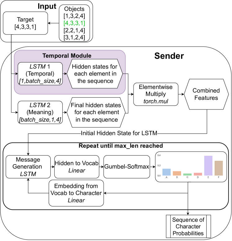
(a) The sender architecture.

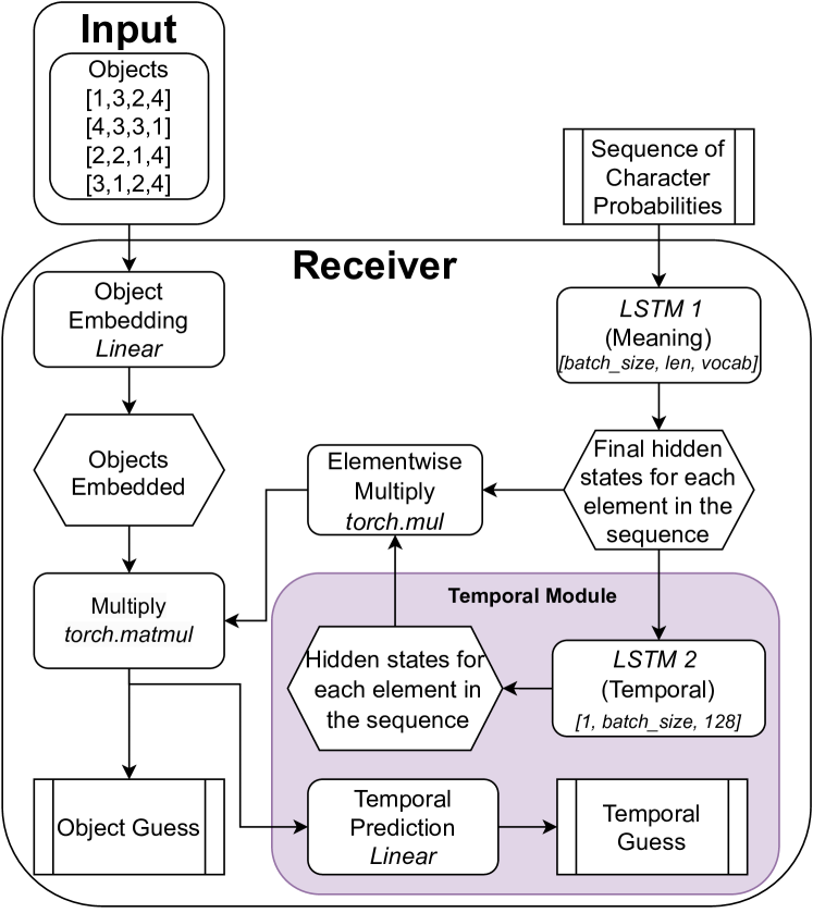
(b) The receiver architecture.

Figure 1: The sender and receiver architectures, with the temporal modules highlighted in purple.

These messages are then passed to the receiver, an overview of which is shown in Figure 1(b). The receiver’s architecture is the same as the EGG framework (Kharitonov et al., 2019), except for the temporal prediction layer and the additional sequential LSTM. The receiver’s sequential LSTM processes messages similarly to how the sender’s sequential LSTM processes objects. First, a hidden state is computed for each message by a regularly batched LSTM. Then, the sequential LSTM processes each of the regularly batched LSTM’s hidden states to build a temporal understanding of the sender’s messages. The temporal prediction layer, in turn, allows the agent to signify whether an object is the same as a previously seen object, up to the previous horizon $h$. This is implemented as a single linear layer, which outputs the temporal label prediction. For example, if an object was last seen $4$ episodes ago, the output of the temporal prediction layer should also be $4$.The temporal label used in this loss function only considers the previous horizon $h$; otherwise, it defaults to $0$. For example, assume an object has been repeated in the current episode and has last appeared $5$ episodes ago. If the previous horizon $h$ is 8, the label assigned to this object would be $5$, as $5$ past episodes are still within the horizon, $5\leq h$. However, if $h$ is 4, the label would be $0$, as the episode lies outside the previous horizon, $4\geq h$.

This predictive ability is combined with an additional term in the loss function, which together form a temporal loss. The temporal loss can be formulated as $L_{t}=L_{rg}+L_{tp}$. The $L_{rg}$ component is the classic referential game loss between the receiver guess and the sender target label, using cross entropy. $L_{tp}$ is the temporal prediction loss, which is implemented using cross entropy between the labels of when an object has last appeared, and the receiver’s prediction of that label. Agents that include this loss perform an additional task, which corresponds to correctly identifying which two outputs are the same. The goal of this loss is to improve the likelihood of an agent developing temporal references by increasing the focus on these relationships. Analysis of how the presence of this explicit loss impacts the development of temporal references is provided in Section 3.

3 Temporality Experiments

3.1 Temporality Metric

We propose a metric, denoted as $M_{\ominus^{n}}$, which measures how often a given message has been used as the “previous” operator in prior communication. Given a sequence of objects shown to the sender and messages sent to the receiver $\tau$, it checks when an object has been repeated within a given horizon $h_{v}$, and records the corresponding message sent to describe that object.

Let $C_{m}{\ominus^{n}}$ count the times the message $m$ has been sent together with a repeated object for $h_{v}=n$:

$$C_{m}{\ominus^{n}}=\sum_{n=1}^{t}\mathbb{I}(m_{n}=m\land\text{objectRepeated}(x_{n},h_{v}))$$ (3)

where $\mathbb{I}(\cdot)$ is the indicator function that returns 1 if the condition is true and 0 otherwise, and $\text{objectRepeated}(x_{n},h_{v})$ is a function that evaluates to true if the object $x_{n}$ is the same as the object $h_{v}$ episodes ago.

Let $C_{m}{\text{total}}$ denote the total count of times the message $m$ has been used:

$$C_{m}{\text{total}}=\sum_{n=1}^{t}\mathbb{I}(m_{n}=m)$$ (4)

where $\mathbb{I}(\cdot)$ is an indicator function selecting the message $m$ in the exchange history $\tau$.

The percentage of previous messages that are the same as $m$ can then be calculated using $M_{\ominus^{n}}(m)$:

$$M_{\ominus^{n}}=\frac{C_{m}{\ominus^{n}}}{C_{m}{\text{total}}}\times 100$$ (5)

To give intuition to this metric, its objective is to measure if a message is used similarly to the natural language sentence “The car I can see is the same colour as the one mentioned two sentences ago”, if the message can give reference to a previous episode. More formally, assume a target object sequence of $[1,2,3,2,2,2,1]$. For simplicity, a single attribute is assigned per object, with only one object repeating: $2$. We can then consider three message sequences: $[1,2,3,2,4,4,1]$, $[1,2,3,4,4,4,1]$ and $[1,2,3,2,2,2,1]$, and calculate our metric for $\ominus^{1}$.

There are two repetitions in the sequence of objects: the second and third $2$ following the sequence of $[1,2,3,2]$. In the first example message sequence, for both of the repetitions, the message $4$ has been sent and so $C_{m}{\ominus^{1}}=2$. The total use of $4$ is $C_{m}{\text{total}}=2$. Calculating the metric $M_{\ominus^{1}}=2/2\times 100=100\%$ gives $100\%$ for the use of $4$ as a $\ominus^{1}$ operator. The result of $100\%$ indicates that this message is used exclusively as a $\ominus^{1}$ operator.

In the second message sequence, $4$ has also been used for the initial observation of the object. This means that $C_{m}{\text{total}}=3$, while $C_{m}{\ominus^{1}}=2$. We can calculate $M_{\ominus^{1}}=2/3\times 100=66\%$, which shows the message being used as $\ominus^{1}$ $66\%$ of the time.

Lastly, the simplest case of a message describing an object exactly. Following the previous examples, $C_{m}{\text{total}}=4$, with $C_{m}{\ominus^{1}}=2$. This message would then be classed as $50\%$ $\ominus^{1}$ usage, $M_{\ominus^{1}}=2/4\times 100=50\%$. A non-$100\%$ result indicates that the message is not used exclusively as a $\ominus^{1}$ operator. For any result lower than $100\%$ on the $M_{\ominus^{n}}$ metric, the message is excluded as being a $\ominus^{n}$ operator. This is a strong requirement as it omits messages that are not used consistently.

3.2 Agent Training

The following architectures are evaluated:

Non-Temporal-NL

(NL meaning No-Loss) The same as regular emergent communication agents, which is used as a baseline for comparison;

Non-Temporal

The same as regular emergent communication agents, but with temporal loss;

Temporal-NL

Includes the sequential LSTM, but not the temporal loss; and

Temporal

Includes both the sequential LSTM and the temporal loss.

The agents that include the temporal loss (Temporal and Non-Temporal) have an explicit reward to develop temporal understanding. There is no additional pressure to develop temporal references for agents that do not include the temporal loss (Temporal-NL and Non-Temporal-NL), except for the possibility of increased performance on the referential task.

We hypothesise that Non-Temporal, Temporal-NL and Temporal agents will develop temporal references, with the Temporal agents more likely to do so, given their incentive is higher. This means that we should see our $M_{\ominus^{n}}$ metric reach $100\%$ for all these agents, but not for the Non-Temporal-NL agents.

All agent types were trained for the same number of epochs and on the same environments during each run. Evaluation of the network checkpoints is performed after the training has finished. Each agent pair is assessed in the six different environments: “Always Same”, “Never Same”, “RG Classic”, “RG Hard”, “TRG Previous” and “TRG Hard”. The target objects are uniformly sampled from the object space $V$ in all environments.

Each possible configuration was run ten times with randomised seeds between runs for both the agents and the datasets. Each agent pair was then evaluated in six different environments. Appendix A provides further details.

3.3 Temporality Analysis

Figure 2(a) illustrates the $M_{\ominus^{4}}$ metric values (referring to an observation four messages in the past) of all agent types over the evaluation environments (Sections 3.2 and 3.1), where $M_{\ominus^{4}}\geq 0\text{\%}$ . It indicates that the change in architecture makes the agents predetermined to develop temporal references. Only the networks that have the sequential LSTM, Temporal and Temporal-NL, are capable of producing temporal references. Conversely, temporal references emerge in both Temporal and Temporal-NL networks, regardless of the training dataset. This shows that even in a regular environment, without additional pressures, temporal references are advantageous. No messages in the Non-Temporal or Non-Temporal-NL architectures are used $100\%$ of the time for $\ominus^{4}$, irrespective of the dataset they have been trained on. This demonstrates that the temporal loss is not enough, and that a sequential LSTM module is the key factor to the emergence of temporal references.

Figure 2(b) shows that messages that are used for $\ominus^{4}$ have a high chance of being correct, with most averaging above 90% correctness. Correctness refers to whether the receiver agent correctly guessed the target object after receiving the message. As expected, no Non-Temporal networks appear in Figure 2(b) because they learn no temporally specialised messages, and so no messages are used as $\ominus^{4}$.

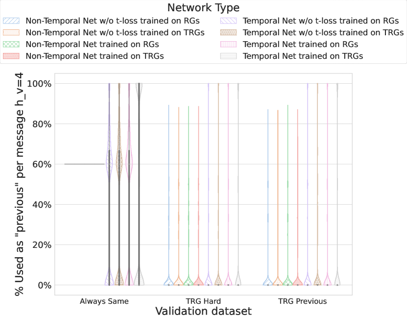
(a)

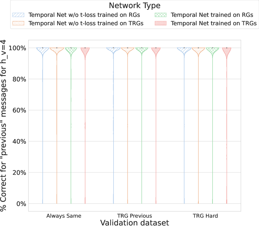
(b)

Figure 2: The $M_{\ominus^{4}}$ metric (2(a)) and correctness of messages (2(b)) used as the $\ominus^{4}$ operator.

Analysing the development of temporal references, we observe the emergence of messages being used by the agents to describe the previous $h_{v}=4$ episodes. As an example of such behaviour, in one of the runs where the agents were trained in the Temporal configuration, the message $[25,6,9,3,2]$ was consistently used as a $\ominus^{1}$ operator. When the agents were evaluated in the “Always Same” environment, they used this message only when the target objects were repeating, while also being used exclusively for twelve distinct objects. For a total of 10 repetitions of each object, this message was utilised nine times, indicating that the only time a different message was sent was when the object appeared for the first time. For example, when the object $[4,2,3,6,5,8,8,4]$ appeared for the first time, a message $[25,6,17,9,9]$ was sent, and subsequently the temporal message was used. This shows that temporal messages aid generalisation. A message that has been developed in a different training environment, in this case “TRG Previous”, can be subsequently used during evaluation, even if the targets are not shared between the two environments.

The distribution of all messages as compared to their $M_{\ominus^{4}}$ value is shown in Figure 3(a). Most messages are used only in the context of the current observations, with both Temporal and Temporal-NL networks using a more specialised subset of messages to refer to the temporal relationships. Only Temporal and Temporal-NL variants develop messages that reach $100\%$ on the $M_{\ominus^{4}}$ metric. The distribution also suggests that these messages could be a more efficient way of describing objects, as the number of temporal messages is relatively small. With parsimony incentives applied to the networks, these could be shortened (Rita et al., 2020), which would allow the agents to communicate with more bandwidth efficiency.

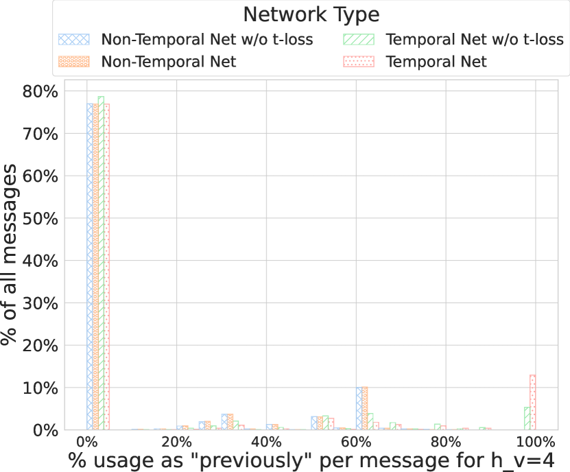
(a)

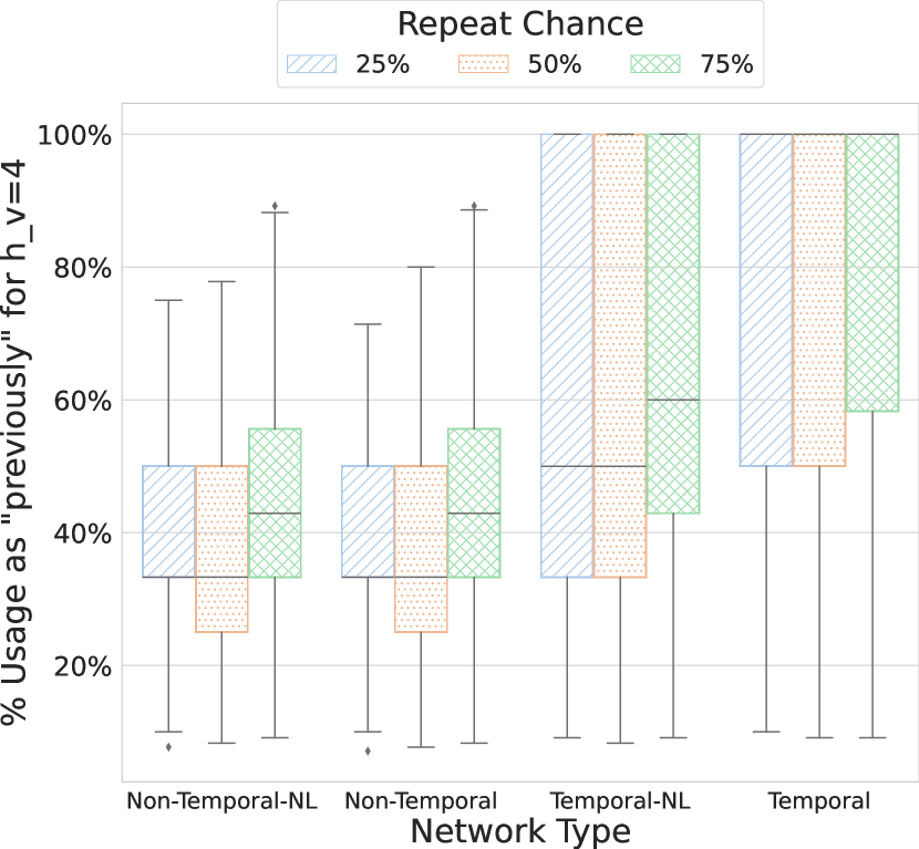
(b)

Figure 3: Usage of messages compared to their $M_{\ominus^{4}}$ value (3(a)), and of the $M_{\ominus^{4}}$ value when varying the network type and the chance of repetition (3(b)).

The percentage of networks that develop temporal messaging is shown in Table 1. The percentages shown are absolute values, calculated by taking the total number of runs and checking whether at least one message has reached $M_{\ominus^{n}}=100\text{\%}$ for each run. Then that number of runs is divided by the total number of runs of the corresponding configuration to arrive at the quantities in Table 1.

In Table 1, both Temporal and Temporal-NL network variants reach over $95\%$ of runs that have converged to a strategy which uses at least one message as the $\ominus^{n}$ operator. In contrast, the Non-Temporal and Non-Temporal-NL networks never achieve such a distinction. Additionally, some runs have not converged to a temporal strategy in the case of both Temporal network variants. However, these experiments account for only $3\%$ of the total number of runs. These results further show that the presence of a sequential LSTM is the deciding factor in the emergence of temporal references. Only networks that include the sequential LSTM converge to strategies that include such references.

To thoroughly investigate this result, we analyse the impact of the network size on the development of temporal references. We evaluate agents with just the temporal module, removing the Meaning LSTM 2 for the sender and the Meaning LSTM 1 for the receiver, matching the number of parameters as observed in the base agent (Section 2.4). The agents with just the temporal module still develop temporal references, but perform worse on the referential task, achieving lower accuracy. Therefore, they are omitted them from the comparisons in this section.

Table 1: Percentage of networks that develop temporal messages.

Network Type	Loss Type	Percentage
Non-Temporal	Non-Temporal	$0\%$
Non-Temporal	Temporal	$0\%$
Temporal	Non-Temporal	$100\%$
Temporal	Temporal	$100\%$

4 Discussion

When and how can temporal references emerge? We posit that our addition of the sequential LSTM to the agents is key to allowing them to develop the ability to communicate about time. The fundamental factor in the emergence of temporal references is whether the agents can look into the past, which the sequential LSTM allows them to do. Our results support this, showing the inclusion of this module is sufficient for agents to form temporal references.

In Figure 3(b), we verify that by increasing the number of repetitions in a dataset, the use of temporal messages increases. As we increase the repetition chance, the percentage of messages that are used for $\ominus^{n}$ increases for all agent variants. On average, Non-Temporal and Non-Temporal-NL networks demonstrate the same chance of using a message for $\ominus^{n}$ as the dataset repetition chance. This means that while the percentage increases, it is only due to the increase in the repetition chance. If a dataset contains 75% repetitions, on average, each message will be used as an accidental $\ominus^{n}$ 75% of the time. For example, if the language does not have temporal references and uses a given message to describe an object, this message will be repeated every time this object appears. This means that for every repetition, the message could be seen as a message indicating a previous episode, whereas in reality, it is just a description of the object. In contrast to Non-Temporal and Non-Temporal-NL networks, for Temporal and Temporal-NL networks, the average percentage does reach 100%. This means that messages the agents designate for $\ominus^{n}$ are used more often than the repetition chance.

Our results also indicate that the only pressures required for temporal messages to emerge are implicit, and that no explicit pressures are required. We show that the incentives are already present in datasets that are not altered to increase the number of repetitions occurring. Temporal references therefore emerge naturally, as long as the agents are equipped with a temporal module, such as the sequential LSTM used in our work. This ease of transfer of our architectural insights allows temporal references to emerge in any emergent communication settings. It could allow for greater bandwidth efficiency by allowing agents to use shorter messages for events that happen often, especially when combined with other linguistic parsimony approaches (Rita et al., 2020; Chaabouni et al., 2019).

The emergence of temporal references only through architectural changes could also point towards additional insights in terms of modelling human language evolution using EC (Galke et al., 2022). Our sequential LSTM approach to the emergence of temporal references could be viewed as analogous to sequential learning in natural language (Christiansen and Kirby, 2003), as we learn to encode and represent elements in temporal sequences.

5 Limitations

It’s possible for the agent to send a unique message that describes the time of the object’s appearance, rather than sending a message it has used before. Our metric would then incorrectly identify the training run as having no temporal references, given that all messages generated would be unique. This would require the agents to develop a very large vocabulary, creating a unique message for every object repetition. We do not, however, observe this happening in our training runs, as our agents’ vocabulary contains at most 4k unique messages over the whole training run. This is significantly smaller than the number of repeated objects, which in the case of the $50\%$ repetition dataset would be 10k. Using the pigeonhole principle, we can conclude that they do not create a unique message for each object repetition. We consider that this limitation is related to the issues with most compositionality metrics in EC. While most compositionality metrics measure trivial compositionality (Chaabouni et al., 2020; Ueda et al., 2022; Perkins, 2021), our metric would be akin to measuring trivial temporality.

6 Conclusion

Discussing past observations is vital to communication, saving bandwidth by avoiding repeating information and allowing for easier experience sharing. We investigate the emergence of temporal references, addressing the fundamental questions of when and how they can develop. We present an environment to probe how agents might create such references. By testing environmental pressures, employing multiple network architectures, and incorporating a temporal referencing reward, we analyse the mechanisms underlying the formation of temporal references.

We perform a comparison of a conventional agent architecture with an architecture featuring a sequentially batched LSTM. We show that a new architecture with a different batching strategy is sufficient for temporal references to emerge, finding the additional explicit incentive of a temporal loss to be unnecessary. The ability to process observations temporally through the sequential LSTM, combined with implicit pressures from the environment, allows temporal references to emerge naturally.

Acknowledgments and Disclosure of Funding

This work was supported by the UK Research and Innovation Centre for Doctoral Training in Machine Intelligence for Nano-electronic Devices and Systems [EP/S024298/1].

The authors would like to thank Lloyd’s Register Foundation for their support.

The authors acknowledge the use of the IRIDIS High-Performance Computing Facility, and associated support services at the University of Southampton, in the completion of this work.

Appendix A Training Details

Our agents were trained using PyTorch Lightning (Falcon and The PyTorch Lightning Team, 2019) using the Adam optimizer (Kingma and Ba, 2015), with experiment tracking done via Weights & Biases (Biewald, 2020). We provide our grid search parameters per network and per training environment in Table 2. We ran a manual grid search over these parameters for each network and training dataset combination, where the networks were Non-Temporal, Non-Temporal-NL, Temporal, and Temporal-NL, and the training datasets were Classic Referential Games or Temporal Referential Games. Each trained network was then evaluated on the six available environments: Always Same, Never Same, Classic Referential Games, Temporal Referential Games, Hard Classic Referential Games, and Hard Temporal Referential Games. Running the grid search for one iteration, with the value of repetition chance fixed, took approximately 28 hours, using the compute resources in Table 3.

Table 2: Grid Search Parameters

Parameter	Value
Epochs	[600]
Optimizer	Adam
Learning Rate $\alpha$	0.001
Number of Objects in Dataset	[20 000]
Number of Distractors	[10]
Number of Properties $N_{P}$	[8]
Number of Features $N_{F}$	[8]
Length Penalty	[0]
Maximum Message Length $L$	[5]
Vocabulary Size $S$	[26]
Repetition Chance	[0.25, 0.5, 0.75]
Previous Horizon $h$	[8]
Sender Embedding Size	[128]
Sender Meaning LSTM Hidden Size	[128]
Sender Temporal LSTM Hidden Size	[128]
Sender Message LSTM Hidden Size	[128]
Receiver LSTM+Linear Hidden Size	[128]
Gumbel-Softmax Temperature	[1.0]

Table 3: Compute Resources

Resource	Quantity
CPU Cores (Intel(R) Xeon(R) Silver 4216 × 2)	20
GPUs (NVIDIA Quadro RTX8000)	1
Wall Time	28hrs

Appendix B Datasets Details

In Figure 4, we analyse our datasets, using the parameters as specified in Appendix A, for the number of repetitions that occur. When the temporal dataset repetition chance is set to 50%, the datasets, predictably, oscillate around 50% of repeating targets. Generating the targets randomly yields a miniscule fraction of repetitions of less than 1%, as we can see in Figure 4, for the Classic and Hard referential games.

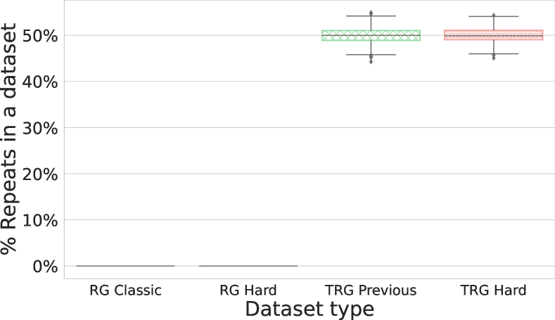
Figure 4: Number of target repetitions per dataset. Regular referential games datasets very rarely encounter target repetitions. This data is an average over 1000 seeds per environment.

B.1 Test Environments

Both “Always Same” and “Never Same” environments act as sanity checks for our results.

We provide example inputs and outputs for both environments in Table 4. We use single-property objects and messages for clarity.

For the “Always Same” environment, in the case of the agent using temporal references, we may also see other messages instead of the message 4, as we have observed that there are more than one message used as previously. We always expect to see at least 90% of usage as previously for this environment. However, for agents that learn temporal referencing strategies, we would expect the usage to reach 100%.

For the “Never Same” environment, we expect to see no temporal references being identified. Any identification of temporal references in the Never Same environment would indicate an issue with our metric.

Table 4: Example Inputs and Outputs for both of our test environments.

Environment	Input	Temporal Referencing	No Temporal Referencing
Always Same	[1,1,1,2,2,2,3,3,3]	[1,4,4,2,4,4,3,4,4]	[1,1,1,2,2,2,3,3,3]
Never Same	[1,2,3,4,5,6,7,8]	[1,2,3,4,5,6,7,8]	[1,2,3,4,5,6,7,8]

Appendix C Architecture Overview

In Figure 5, we present an overview of our whole experimental setup. We can see the sender and receiver architectures, together with their inputs, as described in Section 2.4. We also show our loss calculations, for both the Temporal-NL version and the Temporal version of our games. In the Temporal-NL variant, we disable the temporal prediction module for the receiver, also disabling the temporal loss. Consequently, in the Non-Temporal version we disable both the temporal loss and the sequential LSTM, to achieve an architecture as close as possible to the ones used in most emergent communication research (Kharitonov et al., 2019).

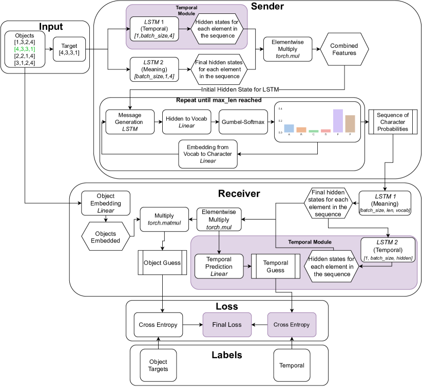
Figure 5: Full overview of our Temporal Referential Games setup. Together with the sender and receiver we have described in Section 2.4, we also include the working of the loss.

Appendix D Accuracy Analysis

We compare the accuracy of both variants of the Temporal networks to Non-Temporal networks in Figure 6. According to this metric, the Temporal networks with the temporal loss perform marginally worse than the networks which do not include the temporal predictions. Temporal-NL networks that do not need to output temporal predictions, and so are not incentivised to assign more weight to the temporal aspects, perform better, matching the performance of the regular agents. Additionally, using the comparison between “RG Classic” and “RG Hard” (and analogously “TRG Previous” and “TRG Hard”), we observe that temporal references do not improve the performance on harder tasks, where targets are highly similar.

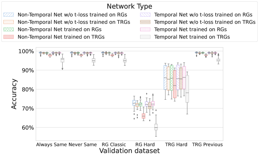
Figure 6: The evaluation accuracies for all of our network types, in all of our evaluation environments.

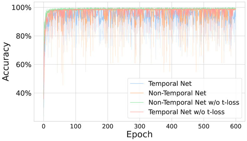
Figure 7: Average validation accuracy across all training and validation environments for all of our network types versus the number of epochs trained. All runs converge to close to 100% accuracy, and we observe no reduction in accuracy over longer training times.

We believe that the reason for the accuracy drop lies in too much pressure on the temporal aspects in the case of networks that include a loss for temporal predictions. Because of this additional loss, the agents can increase their rewards by only focusing on creating temporal messages, without learning a general communication protocol. This then leads to an overfit to the training dataset, where they can rely on both their mostly temporal language and their memory of the object sequences, instead of communicating about the object properties. Consequently, we observe a decline in performance on the evaluation dataset.

We also found no overfitting of our agents, even over 600 epochs of training, as their evaluation accuracy does not decrease. We find that our agents continue to hold at approximately 100% accuracy, even 500 epochs after they have reached peak performance, which we can see in Figure 7. This contrasts with a recent result in Rita et al. (2022), where agents were reported to overfit as training passed 250 epochs. As our Temporal-NL networks do not experience this decrease in accuracy, it may point to an advantage of temporal communication in countering co-adaptation of agents. However, the setting used in Rita et al. (2022) is different from ours, as the authors focus their analyses on a reconstruction game, where agents are tasked with reconstructing the sender input given a message. Instead, in our game, agents are asked to pick the correct object from a list. Another possible factor we have identified is the model size difference between our setting and Rita et al. (2022). While we use a hidden size of 128 for the LSTM, Rita et al. (2022) use 256. This is another possible reason for the observed overfitting, as it is well-known that larger models tend to overfit more easily. This may be in addition to the regularising impact of the environment or the temporal loss.

Appendix E Message Clustering

We show example t-SNE (Maaten and Hinton, 2008) clusterings of messages from two different evaluation runs in Figure 8 and Figure 9. In Figure 8, we observe that the messages are spread apart, indicating that they are not likely to be compositional. In Figure 9, the messages are clustered together, which may indicate that they share a common part and are therefore compositional.

Figure 8: Messages clustered using the t-SNE technique. All messages are spread out, indicating they are unlikely to be compositional.

Figure 9: Messages clustered using the t-SNE technique. Some messages are clustered together, indicating they may be compositional.

Appendix F Analysis for previous horizon from $h_{v}=1$ to $h_{v}=8$

In this section, we present the additional results for previous horizon from $h_{v}=1$ to $h_{v}=8$.

Table 5: Emergence of temporal references for a given horizon

Network Type	$h_{v}=1$	$h_{v}=2$	$h_{v}=3$	$h_{v}=4$	$h_{v}=5$	$h_{v}=6$	$h_{v}=7$	$h_{v}=8$
Non-Temporal-NL	0%	0%	0%	0%	0%	0%	0%	0%
Non-Temporal	0%	0%	0%	0%	0%	0%	0%	0%
Temporal-NL	99.44%	100%	100%	99.72%	98.61%	100%	99.72%	98.89%
Temporal	99.72%	100%	99.72%	99.17%	99.44%	99.72%	99.72%	99.44%

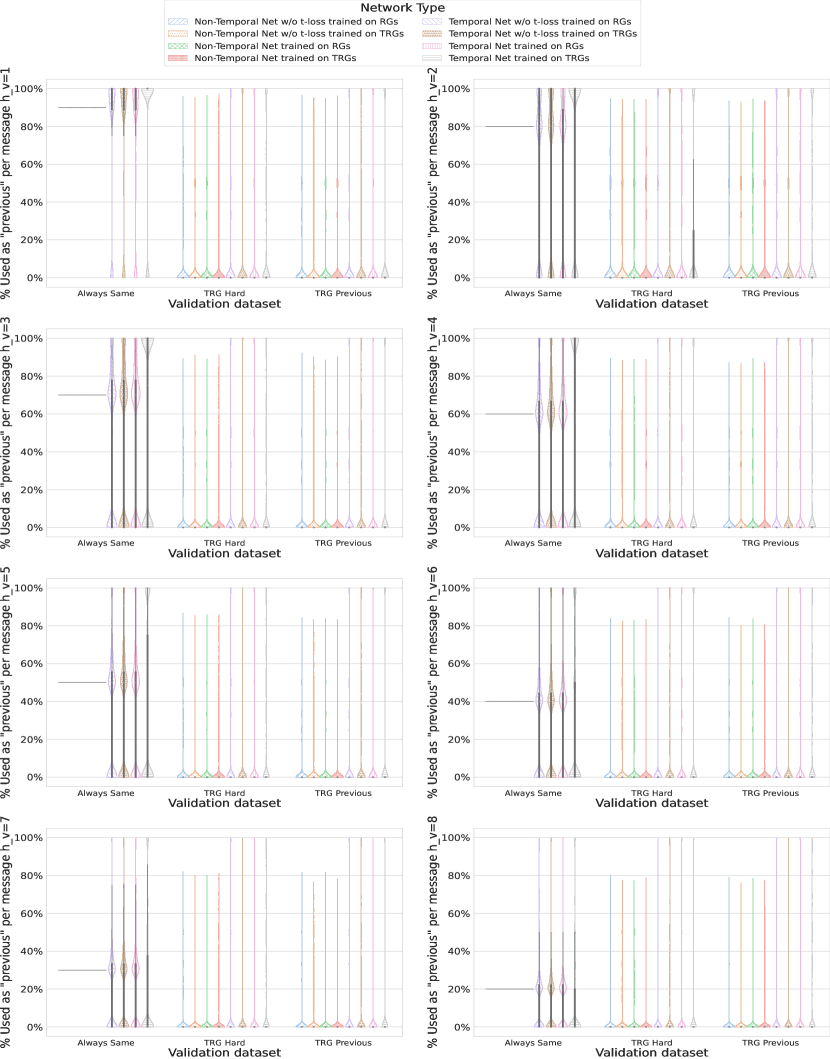
Figure 10: The $M_{\ominus^{h}}$ metric values per message, for all environments where $M_{\ominus^{h}}\geq 0\text{\%}$.

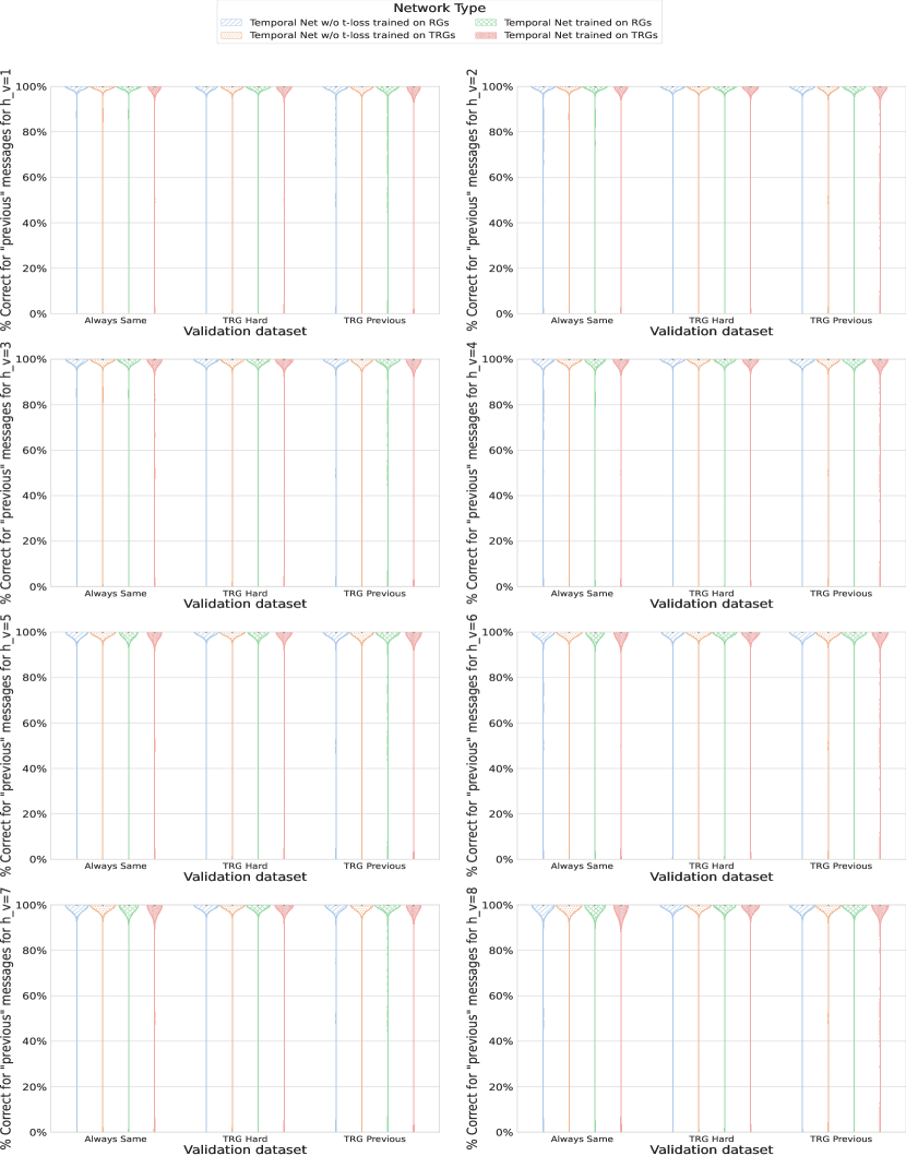
Figure 11: Correctness of messages used as the $\ominus^{h}$ operator.

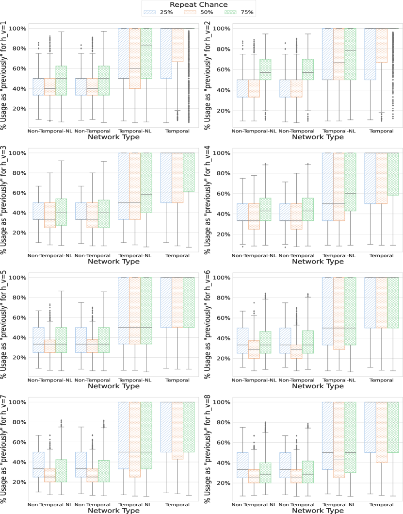
Figure 12: The $M_{\ominus^{h}}$ value when varying the network type and the chance of repetition.

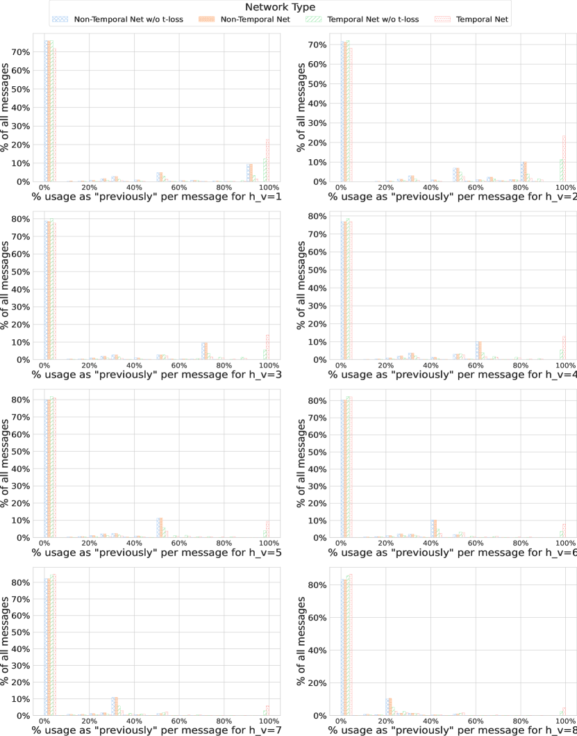
Figure 13: Usage of messages compared to their $M_{\ominus^{h}}$ value.

References

- Auersperger and Pecina (2022) Michal Auersperger and Pavel Pecina. Defending compositionality in emergent languages. In Proceedings of the 2022 Conference of the North American Chapter of the Association for Computational Linguistics: Human Language Technologies: Student Research Workshop, pages 285–291. Association for Computational Linguistics, 2022.
- Biewald (2020) Lukas Biewald. Experiment Tracking with Weights and Biases, 2020.
- Bosc (2022) Tom Bosc. Varying meaning complexity to explain and measure compositionality. In Emergent Communication Workshop at ICLR 2022, 2022.
- Chaabouni et al. (2019) Rahma Chaabouni, Eugene Kharitonov, Emmanuel Dupoux, and Marco Baroni. Anti-efficient encoding in emergent communication. In Advances in Neural Information Processing Systems 32: Annual Conference on Neural Information Processing Systems 2019, NeurIPS 2019, December 8-14, 2019, Vancouver, BC, Canada, pages 6290–6300, 2019.
- Chaabouni et al. (2020) Rahma Chaabouni, Eugene Kharitonov, Diane Bouchacourt, Emmanuel Dupoux, and Marco Baroni. Compositionality and generalization in emergent languages. In Proc. of ACL, pages 4427–4442. Association for Computational Linguistics, 2020.
- Chaabouni et al. (2022) Rahma Chaabouni, Florian Strub, Florent Altché, Eugene Tarassov, Corentin Tallec, Elnaz Davoodi, Kory Wallace Mathewson, Olivier Tieleman, Angeliki Lazaridou, and Bilal Piot. Emergent communication at scale. In Proc. of ICLR. OpenReview.net, 2022.
- Cho et al. (2014) Kyunghyun Cho, Bart van Merriënboer, Dzmitry Bahdanau, and Yoshua Bengio. On the properties of neural machine translation: Encoder–decoder approaches. In Proceedings of SSST-8, Eighth Workshop on Syntax, Semantics and Structure in Statistical Translation, pages 103–111. Association for Computational Linguistics, 2014.
- Christiansen and Kirby (2003) Morten H. Christiansen and Simon Kirby. Language evolution: consensus and controversies. Trends in Cognitive Sciences, 7(7):300–307, 2003. ISSN 1364-6613.
- Falcon and The PyTorch Lightning Team (2019) William Falcon and The PyTorch Lightning Team. PyTorch Lightning, 2019.
- Galke et al. (2022) Lukas Galke, Yoav Ram, and Limor Raviv. Emergent Communication for Understanding Human Language Evolution: What’s Missing? In Emergent Communication Workshop at ICLR 2022, 2022.
- Hochreiter and Schmidhuber (1997) Sepp Hochreiter and Jürgen Schmidhuber. Long Short-Term Memory. Neural Computation, 9(8):1735–1780, 1997. ISSN 0899-7667.
- Jang et al. (2017) Eric Jang, Shixiang Gu, and Ben Poole. Categorical reparameterization with gumbel-softmax. In Proc. of ICLR. OpenReview.net, 2017.
- Kalinowska et al. (2022a) Aleksandra Kalinowska, Elnaz Davoodi, Kory W. Mathewson, Todd Murphey, and Patrick M. Pilarski. Towards Situated Communication in Multi-Step Interactions: Time is a Key Pressure in Communication Emergence. Proceedings of the Annual Meeting of the Cognitive Science Society, 44(44), 2022a.
- Kalinowska et al. (2022b) Aleksandra Kalinowska, Elnaz Davoodi, Florian Strub, Kory Mathewson, Todd Murphey, and Patrick Pilarski. Situated Communication: A Solution to Over-communication between Artificial Agents. In Emergent Communication Workshop at ICLR 2022, 2022b.
- Kang et al. (2020) Yipeng Kang, Tonghan Wang, and Gerard de Melo. Incorporating pragmatic reasoning communication into emergent language. In Advances in Neural Information Processing Systems 33: Annual Conference on Neural Information Processing Systems 2020, NeurIPS 2020, December 6-12, 2020, virtual, 2020.
- Kharitonov et al. (2019) Eugene Kharitonov, Rahma Chaabouni, Diane Bouchacourt, and Marco Baroni. EGG: a toolkit for research on emergence of lanGuage in games. In Proc. of EMNLP, pages 55–60. Association for Computational Linguistics, 2019.
- Kingma and Ba (2015) Diederik P. Kingma and Jimmy Ba. Adam: A method for stochastic optimization. In Proc. of ICLR, 2015.
- Lazaridou and Baroni (2020) Angeliki Lazaridou and Marco Baroni. Emergent Multi-Agent Communication in the Deep Learning Era. ArXiv preprint, abs/2006.02419, 2020.
- Lazaridou et al. (2017) Angeliki Lazaridou, Alexander Peysakhovich, and Marco Baroni. Multi-agent cooperation and the emergence of (natural) language. In Proc. of ICLR. OpenReview.net, 2017.
- Lazaridou et al. (2018) Angeliki Lazaridou, Karl Moritz Hermann, Karl Tuyls, and Stephen Clark. Emergence of linguistic communication from referential games with symbolic and pixel input. In Proc. of ICLR. OpenReview.net, 2018.
- Lewis (1969) David Kellogg Lewis. Convention: A Philosophical Study. Cambridge, MA, USA: Wiley-Blackwell, 1969.
- Lichtenstein et al. (1985) Orna Lichtenstein, Amir Pnueli, and Lenore Zuck. The glory of the past. In Workshop on Logic of Programs, pages 196–218. Springer, 1985.
- Lipinski et al. (2022) Olaf Lipinski, Adam Sobey, Federico Cerutti, and Timothy J. Norman. Emergent Password Signalling in the Game of Werewolf. In Emergent Communication Workshop at ICLR 2022, 2022.
- Maaten and Hinton (2008) Laurens van der Maaten and Geoffrey Hinton. Visualizing Data using t-SNE. Journal of Machine Learning Research, 9(86):2579–2605, 2008. ISSN 1533-7928.
- Maler et al. (2008) Oded Maler, Dejan Nickovic, and Amir Pnueli. Checking Temporal Properties of Discrete, Timed and Continuous Behaviors. In Pillars of Computer Science: Essays Dedicated to Boris (Boaz) Trakhtenbrot on the Occasion of His 85th Birthday, Lecture Notes in Computer Science, pages 475–505. Springer, 2008. ISBN 978-3-540-78127-1.
- Ossenkopf et al. (2019) Marie Ossenkopf, Mackenzie Jorgensen, and Kurt Geihs. When Does Communication Learning Need Hierarchical Multi-Agent Deep Reinforcement Learning. Cybernetics and Systems, 50(8):672–692, 2019. ISSN 0196-9722.
- Perkins (2021) Hugh Perkins. Neural networks can understand compositional functions that humans do not, in the context of emergent communication. ArXiv preprint, abs/2103.04180, 2021.
- Pnueli (1977) Amir Pnueli. The temporal logic of programs. In 18th Annual Symposium on Foundations of Computer Science (sfcs 1977), pages 46–57. ieee, 1977.
- Rita et al. (2020) Mathieu Rita, Rahma Chaabouni, and Emmanuel Dupoux. “LazImpa”: Lazy and impatient neural agents learn to communicate efficiently. In Proceedings of the 24th Conference on Computational Natural Language Learning, pages 335–343. Association for Computational Linguistics, 2020.
- Rita et al. (2022) Mathieu Rita, Corentin Tallec, Paul Michel, Jean-Bastien Grill, Olivier Pietquin, Emmanuel Dupoux, and Florian Strub. Emergent Communication: Generalization and Overfitting in Lewis Games. In Advances in Neural Information Processing Systems 36: Annual Conference on Neural Information Processing Systems 2022, NeurIPS 2022, 2022.
- Spronck and Casartelli (2021) Stef Spronck and Daniela Casartelli. In a Manner of Speaking: How Reported Speech May Have Shaped Grammar. Frontiers in Communication, 6:150, 2021. ISSN 2297-900X.
- Taillandier et al. (2023) Valentin Taillandier, Dieuwke Hupkes, Benoît Sagot, Emmanuel Dupoux, and Paul Michel. Neural Agents Struggle to Take Turns in Bidirectional Emergent Communication. 2023.
- Ueda and Washio (2021) Ryo Ueda and Koki Washio. On the relationship between Zipf’s law of abbreviation and interfering noise in emergent languages. In Proc. of ACL, pages 60–70. Association for Computational Linguistics, 2021.
- Ueda et al. (2022) Ryo Ueda, Taiga Ishii, Koki Washio, and Yusuke Miyao. Categorial Grammar Induction as a Compositionality Measure for Emergent Languages in Signaling Games. In Emergent Communication Workshop at ICLR 2022, 2022.
- Zipf (1949) George Kingsley Zipf. Human behavior and the principle of least effort. Human behavior and the principle of least effort. Addison-Wesley Press, 1949.