Spatio-temporal modeling of co-dynamics of smallpox, measles and pertussis in pre-healthcare Finland

Abstract

Infections are known to interact as previous infections may have an effect on risk of succumbing to a new infection. The co-dynamics can be mediated by immunosuppression or -modulation, shared environmental or climatic drivers, or competition for susceptible hosts. Research and statistical methods in epidemiology often concentrate on large pooled datasets, or high quality data from cities, leaving rural areas underrepresented in literature. Data considering rural populations are typically sparse and scarce, especially in the case of historical data sources, which may introduce considerable methodological challenges. In order to overcome many obstacles due to such data, we present a general Bayesian spatio-temporal model for disease co-dynamics. Applying the proposed model on historical (1820–1850) Finnish parish register data, we study the spread of infectious diseases in pre-healthcare Finland. We observe that measles, pertussis and smallpox exhibit positively correlated dynamics such that any new infection increased mortality in all three diseases, indicating possibly general immunosuppressive effects at population level.

Keywords: spatio-temporal, infection co-dynamics, pertussis, measles, smallpox,
Bayesian analysis

1 Introduction

Infections exist rarely in isolation and their effects on hosts are known to interact and to have both positive and negative relationships between each other (Gupta et al., , 1998; Rohani et al., , 2003; Shrestha et al., , 2013; Mina et al., , 2015; Nickbakhsh et al., , 2019). For example cross immunity may prevent others infecting the host, competition for same resources or susceptible host can have strong effects on epidemics, and sometimes one infection paves a way for another (Gupta et al., , 1998; Rohani et al., , 2003; Graham, , 2008). Perhaps historically the best-known relationship between infections is the immunosuppressive effect of measles on the following pertussis epidemic by increasing the severity of the epidemic (see Coleman, , 2015; Mina et al., , 2015; Noori and Rohani, , 2019). Coinfections of parasites (Graham, , 2008) and viruses and respiratory bacterial infections are well known (e.g., Bakaletz, , 2017), whereas understanding coinfections and cotransmissions of zika, dengue and chikungunya viruses presents a current serious challenge for public health (Vogels et al., , 2019).

Demographic consequences of epidemics are most dramatically seen in large cities and in densely populated areas, which is reflected in the epidemiological research in general (Mueller et al., , 2020). However, as rural areas constitute a large part of most of the countries, the spatio-temporal dynamics of epidemics in populations with low densities deserve more attention (Mueller et al., , 2020). In rural areas populations often consist of loosely connected metapopulations rather than large and epidemiologically more autonomous populations in cities. This has most likely strong repercussions to the drivers of epidemics (Ball et al., , 2015) and also to the co-occurrence of infections. However, these issues are rarely addressed in literature, possibly due to the statistical challenges encountered with sparse and scarce data, as well as the difficulty of modeling the dynamics of several infections simultaneously both in space and time.

The discrepancy between studying dense and sparse populations is evident and can be seen, for example, by comparing our case of rural Finland in 1820-1850 to the seminal research of Rohani et al., (2003). Their study is based on five large European cities, where the weekly number of fatalities frequently exceeds $30$ and even $80$. In our data, the recorded incidents in most of the towns rarely exceed one person per month, as we study a small and mainly agrarian population in the southern part of Finland, with ca. $1.2$ to $1.6$ million individuals (Voutilainen et al., , 2020). The population, without proper healthcare (Saarivirta et al., , 2012), was spread over a vast area in geographically isolated small towns. Based on the data from 1882, population sizes of towns varied between $300$ and $25{,}000$ (Suomenmaan tilastollinen vuosikirja, , 1882; Ketola et al., , 2021). Despite the obvious uncertainty of population censuses during that era (Voutilainen et al., , 2020), the contrast between our data and most of the published datasets is striking. Statistical modeling of such data is problematic due to incomplete information from some locations and the rare occurrence of events, hampering the ability of generally used models to consider several infectious diseases at the same time and on both temporal and spatial scales.

To estimate the spatio-temporal co-dynamics of deaths due to pertussis, measles and smallpox, we build a model that is able to overcome the limitations of our data. The model estimates jointly death probabilities of multiple infections, and hence enables exploring the temporal and spatial dependence structures within and between the infections. Our general Bayesian model consists of a multivariate latent incidence process, a seasonal component, and multiple predictors whose effects may vary between the towns. This allows us to study the dynamics of all the diseases simultaneously using only the incomplete information about the deaths.

2 Materials and methods

2.1 Data

During the study period, 1820–1850, the parishes in Finland kept track, among others, of baptisms, burials and causes of deaths, according to common and long held principles (Pitkänen, , 1977). Even though the death diagnostics were based on symptoms, some infections can be considered to be diagnosed rather accurately due to their characteristic features. These diseases include pertussis (whooping cough), measles and smallpox, which we consider. These infections were the main reason for child mortality, and, overall, they were responsible for approximately $5$, $3$, and $3$ percent of total deaths, respectively, according to our data. Smallpox vaccinations were started in Finland in 1802, and they were slowly progressing during the study period (Briga et al., , 2022). However, general healthcare was almost non-existent as in 1820 there were only $373$ hospital sickbeds for $1.2$ million inhabitants (Saarivirta et al., , 2012).

Our data consist of daily numbers of deaths, classified by the cause of death, between January 1820 and December 1850 from $N=387$ different regions (towns) in mainland Finland with the exclusion of northern areas. The time window is chosen such that there were no major famines, wars, border changes, or other potentially confounding events, which could have altered the geographical partition or the dynamics of the epidemics. The general stability achieved is advantageous in the modeling.

The daily counts of deaths are aggregated over time into a monthly level, decreasing the number of zero observations yet maintaining a reasonable time resolution for observing the spread of diseases on our geographical scale. This yields a total of $T=372$ time points. The reliability of the actual death counts varies considerably both temporally and spatially owing to the heterogeneous quality of the parish records and the cause of death classifications. Moreover, these deficiencies are not necessarily independent of the true number of deaths. About $24\%$ of the data concerning death occurrences in a town and a month are missing, and from $57$ out of the overall $387$ regions there are no observations at all. Nevertheless, our proposed model provides estimates of the monthly probabilities of death also for these towns.

It is also noteworthy that despite the records of baptisms and burials there are no reliable estimates of the population sizes at the town level (Voutilainen et al., , 2020). Hence the intuitive idea of using local relative mortality is unfortunately beyond reach. Because of this and the aforementioned reliability issues—and since most of the counts are still either zero or one even after the aggregation to a monthly level—only the dichotomous knowledge of the death occurrence is used in the analysis.

2.2 Model

We construct a general model to describe the spatial and temporal dependencies both within and between the infections under study. We also want to enable exploiting other relevant information as explanatory variables. In epidemiological context there typically occur spatial or temporal trends or seasonal effects, which can be included as separate components in the model. In our case we model the probability of dying of a disease at a certain town in a certain month. The model consists of a trend, a seasonal effect, and a regression part reflecting the local effects of the previous state of infection in the focal town and its neighboring towns.

Formally, let $y_{i,t}^{d}$ denote an occurrence of a death caused by a disease $d$ in a region $i=1,\,\dots,\,N$ at a time point $t=1,\,\dots,\,T$, where $N$ is the number of regions and $T$ the number of time points. Let $K_{x}^{d}$ indicate the number of explanatory variables $x$, based on the features of the region $i$. Accordingly, $z$ denotes the explanatory variables, and $K_{z}^{d}$ their number, related to the neighborhood of the region $i$. Thus the model for the occurrence of death caused by the disease $d$ occurring in the region $i$, and at the time point $t$, can be written as follows:

$$y_{i,t}^{d}\sim\text{Bernoulli}\!\left(\!\text{logit}^{-1}\!\left(\lambda_{i}^{d}\tau_{t}^{d}+s_{t}^{d}+a_{i}^{d}+b_{i}^{d}\sum_{k=1}^{K_{x}^{d}}\beta_{k}^{d}x_{i,k}^{d}+c_{i}^{d}\sum_{k=1}^{K_{z}^{d}}\gamma_{k}^{d}z_{i,k}^{d}\!\right)\!\!\right)\!\!.$$

Here Bernoulli distribution with a logit link is chosen due to our dichotomous consideration of the occurrences of death, but other distributions with appropriate link functions can be applied for different types of response variables.

The first three terms being summed form a base level, in our case for the probability of death at each town and month. More specifically, the first term consists of the time dependent latent factor $\tau_{t}$, describing the nationwide incidence, or trend, of the disease, and the regional adjustments or loadings $\lambda_{i}$, with respect to the mean level. As in general dynamic factor models, the products $\lambda_{i}\tau_{t}$ are not identifiable without constraints (Bai and Wang, , 2015). Instead of the common approach of fixing one of the loadings $\lambda_{i}$ to 1, we constrain the mean of the loadings to $1$, enabling the interpretation of the factor $\tau_{t}$ as the nationwide incidence level. The second term $s_{t}$ is a monthly seasonal effect, which is the average deviation from the nationwide incidence level, summing up to $0$ over the months. The third term $a_{i}$ is a regional, zero-mean constant reflecting local deviations from the nationwide incidence level $\tau_{t}$ due to unobserved local demographic, geographic, social or other characteristics associated with mortality.

The last two sum terms form the regression part of the model. The first sum includes the covariates $x_{i,k}$ related to the focal region $i$, and the second sum the covariates $z_{i,k}$ related to the neighboring regions. These variables have both nationwide coefficients $\beta$ and $\gamma$, and their local adjustments $b_{i}$ and $c_{i}$ amplifying or diminishing the nationwide level. As the regional constants $a_{i}$, also the multiplicative local adjustments may account for any unobserved heterogeneity between the regions, such as the local population sizes or densities. The adjustment parameter $b_{i}$ reflects the features of the focal region $i$, and $c_{i}$ those of the neighborhood of region $i$ (possibly relative to $i$). We assume that $b_{i}$ is same for all covariates $x_{k}$, and, accordingly, $c_{i}$ for all $z_{k}$, since the underlying regional characteristics modifying the nationwide mortality effects $\beta$ and $\gamma$ do not depend on the covariates.

In our study there are three covariates assigned to the town $i$ and another three to its neighbors for all diseases $d=p,\,m,\,s$, where $p$ stands for pertussis, $m$ measles and $s$ smallpox. The local explanatory variables $x_{i,k}$ are the presences of deaths caused by the three different diseases in the previous month in the focal town, whereas the regional neighborhood predictors $z_{i,k}$ are the averages of the same death presences over the local neighborhood. We define two regions being neighbors when they share a border. By this definition, all the towns have at least one neighbor. Other definitions of neighborhood could be used as well, for example based on the transportation network or distance, leading to weighted averages of death occurrences.

We model the latent factor $\tau_{t}=(\tau_{t}^{p},\,\tau_{t}^{m},\,\tau_{t}^{s})$, the temporal process describing the baseline of the nationwide incidence rates, as an intercorrelated random walk, $\tau_{t+1}\sim\text{N}(\tau_{t},\Sigma)$. Here $\Sigma$ is an unconstrained $3\times 3$ covariance matrix parametrised using the standard deviations $\sigma_{\tau}^{d}$ and the correlation matrix $R$. In our application this latent process, together with the regional constant and the monthly effect, can be interpreted as the probability of new deaths in a particular town when no deaths caused by any of the three diseases were observed in the previous month in the focal town or in its neighborhood.

In the Bayesian modeling framework we need prior distributions for all the parameters to be estimated. The incidence factors $\tau^{d}$ follow a N($-2,2^{2}$) prior at the first time point and form a random walk at later time points. For the correlation matrix $R$ we use LKJ(1) prior with Cholesky parametrisation (Lewandowski et al., , 2009). For the regional parameters we apply Gaussian priors: $\lambda_{i}\sim\text{N}(1,\,\sigma_{\lambda^{d}}^{2}),\,a_{i}\sim\text{N}(0,\,\sigma_{a^{d}}^{2}),\,b_{i}\sim\text{N}(1,\,\sigma_{b^{d}}^{2})$, and $c_{i}\sim\text{N}(1,\,\sigma_{c^{d}}^{2})$. The prior means of the local adjustments $b_{i}$ and $c_{i}$ are set to 1, which enables us to interpret $\beta$ and $\gamma$ as nationwide effects as is the case with additive multilevel models with population-level and group-level effects. While we use a hard equality constraint for the mean of the $\lambda_{i}$s to ensure the identifiability and more efficient estimation of the model, the hierarchical priors for $b$ and $c$ are sufficient for their identifiability. For the unknown deviations $\sigma_{\tau^{d}}$, $\sigma_{\lambda^{d}}$, $\sigma_{a^{d}}$, $\sigma_{b^{d}}$, and $\sigma_{c^{d}}$ we assign Gamma priors with shape parameter $2$ and rate parameter $1$. The nationwide coefficients $\beta$ and $\gamma$ have N($0,\,2^{2}$) priors. The seasonal effects $s_{t}^{d}$ follow a standard normal prior with the aforementioned sum-to-zero constraint. The priors can be seen as weakly informative, and they are chosen primarily to enhance the computational efficiency (Banner et al., , 2020).

Obviously, any of the components in the model could be excluded by setting the corresponding coefficients or standard deviations to zero. Our Bayesian model encompasses all such simplified alternatives, with the corresponding model and parameter uncertainty reflected by the estimated posterior distributions, leading to more truthful uncertainty estimates compared to merely imposing prior constraints on certain effects to be zero.

3 Results

The model is estimated with cmdstanr (Gabry and Češnovar, , 2022), which is an R interface (R Core Team, , 2022) for the probabilistic programming language Stan for statistical inference (Stan Development Team, , 2022). To draw the samples we use NUTS sampler (Hoffman and Gelman, , 2014) with four chains, each consisting of $7{,}500$ iterations, the first $2{,}500$ of which discarded as warm-up. With parallel chains the computation takes about eleven hours. The model is estimated on a supercomputer node with four cores of Xeon Gold 6230 $2.1$ GHz processors and $40$ GB of RAM. According to the standard diagnostics of the cmdstanr (Vehtari et al., , 2021) the model converges. The statistics $\widehat{R}$ are always below $1.004$, and the effective sample sizes are approximately between $800$ and $40{,}000$. The R and Stan codes and the data used for the analysis are available on GitHub (https://anonymous.4open.science/r/infectionDynamics-CEE4).

In order to visualize the temporal and spatial patterns of the death occurrences and to see how the model estimates the death probabilities, the data and the predictions based on the model are plotted as time series and as maps in Figures 1 and 2.

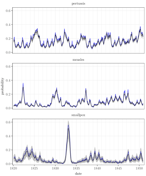
Figure 1: The blue lines illustrate the observed probabilities of a death caused by the diseases, calculated as the proportions of the towns where a death occurred. The black lines show the posterior means of the corresponding estimates and the shaded areas their $95$% posterior intervals.

The temporal behavior of the data and the corresponding estimates are similar. The slight differences may be due to the fact that the proportions are based only on the data available as the model predictions cover all the regions. The spatial patterns of the modeled probabilities reflect the infection distributions visible in the data. Pertussis, measles and smallpox all have emphasis on the eastern half of Finland, with especially measles extending its prevalence to the southern parts of the country as well. By the prediction account, the model seems to work well.

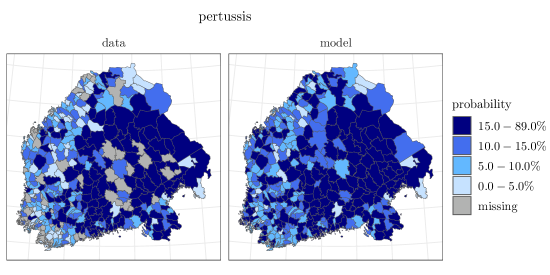
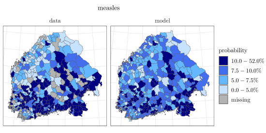
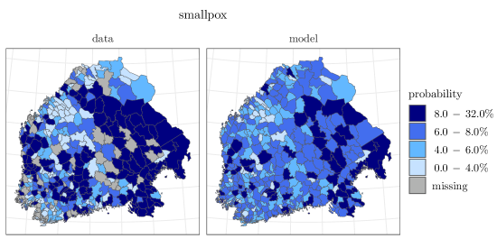
Figure 2: The left panels show the proportions of the months when deaths were recorded over the study period of 31 years. The gray areas indicate the regions where all data are missing. The right panels present the regional averages of the predicted conditional probabilities of death for each month given the actual observations from the previous month. The probabilities are categorized roughly into quartiles of the data for each disease.

In what follows we present the results in detail, which confirms that all the components in the model are relevant, capturing different aspects of the spatio-temporal dynamics of the epidemiological phenomena.

The nationwide incidences of the diseases are depicted by the factors $\tau_{t}^{d}$. The corresponding estimates are shown in Figure 3 on a probability scale. In general, they seem to have the same shapes as the observed nationwide monthly averages of deaths caused by pertussis, measles and smallpox (see Figure 1). There is one major disease outbreak regarding smallpox, whereas the other diseases have several peaks, pertussis varying the most. No clear periodicity can be seen in any of the series, which was also confirmed by estimating dominant frequencies via spectral analysis using the R package forecast (Hyndman and Khandakar, , 2008).

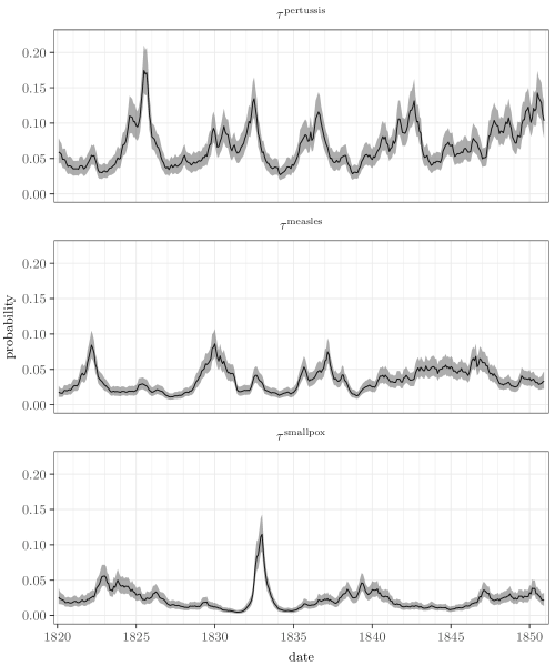
Figure 3: Posterior means and $95$% posterior intervals for the unobserved incidence factors $\tau_{t}^{d}$ for pertussis, measles and smallpox over the time period under study. The curves are on a probability scale.

The seasonal effects $s_{t}^{d}$, or the average monthly deviations from the nationwide incidence level, are shown in Figure 4. According to the estimates, the seasonal effect of pertussis peaks at the beginning of the calendar year, while the effect decreases during the summer and increases again towards the end of the year. In contrast, the only distinctive seasonal effects related to measles and smallpox are the peaks in the spring and the minor decreases at the end of the year.

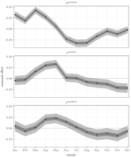
Figure 4: Posterior means (black), $50$% (dark gray) and $95$% (light gray) posterior intervals of monthly seasonal effects $s_{t}^{d}$ for pertussis, measles and smallpox over a year.

Measured by the $\tau$ factors, we found a distinctive correlation between the infections of measles and pertussis, $0.30$ with a $95$% posterior interval $[0.05,\,0.52]$. Omitting the specific seasonal term $s$ in the model yields the same correlation $0.30$ $[0.09,\,0.50]$. The correlation between smallpox and measles is ambiguous, being $0.24$ $[-0.01,\,0.47]$, though it increases to $0.46$ $[0.25,\,0.63]$ in the model without the seasonal component. This implies that monthly effects explain partly but not exhaustively the connection between these diseases. Smallpox and pertussis seem to be mutually independent, $0.03$ $[-0.22,\,0.28]$, which is also the case with the model without the seasonal terms, $0.13$ $[-0.10,\,0.35]$.

According to the regional loadings $\lambda_{i}^{d}$ adjusting the nationwide factors $\tau_{t}^{d}$, it was more likely to die of any of these diseases in eastern and southeastern Finland than in other parts of the study area. This is also in accordance with the maps of the data in Figure 2. The posterior means of the loadings $\lambda$ are plotted in Figure 5. Considering the loadings, there is most local variation in pertussis, $\sigma_{\lambda^{p}}=0.35$ with a $95$% posterior interval $[0.31,0.40]$. With regard to measles and smallpox, the loadings vary less, $\sigma_{\lambda^{m}}=0.17$ $[0.13,0.21]$ and $\sigma_{\lambda^{s}}=0.15$ $[0.13,0.18]$.

The final term affecting the base level of the death probability consists of the regional constants $a_{i}$, shown in Figure 5. Those related to pertussis and smallpox seem to be larger in eastern and southwestern inland areas, whereas those considering measles are largest in southern Finland.

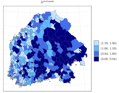
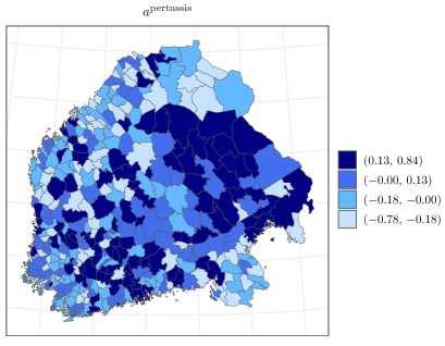
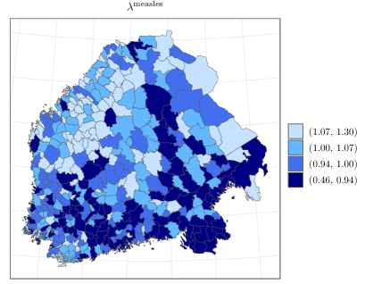
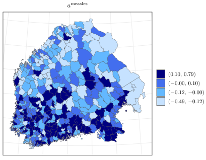
pertussis measles smallpox

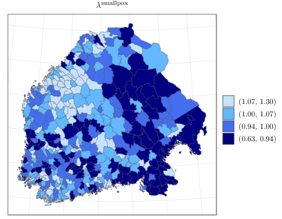
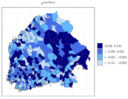
Figure 5: The left panels show the posterior means of the local loadings $\lambda_{i}$, adjusting the national incidence factors $\tau_{t}$, categorized into quartiles. Since the factors are negative, the smaller the loading is, the greater the probability of death is. The right panels illustrate the posterior means of the regional constants $a_{i}$ categorized into quartiles.

The estimates of the nationwide regression coefficients are represented in Table 1. All effects differing from zero are positive, meaning they increase the probability of death. The probability of dying of one of these diseases is increased most prominently if there are recorded deaths caused by the same disease in the same town, or in its neighbors, in the previous month. However, there is more uncertainty in the effects of neighbors than in those of the towns themselves. The risk to die of pertussis is increased by the occurrence of measles, whereas the corresponding effect of smallpox is not distinctive. Measles is probably affected more by smallpox than by pertussis. In turn, measles seems to affect smallpox more than pertussis does.

Table 1: Posterior means and 95% posterior intervals of the nationwide regression parameters grouped by the response disease. Superscript indicates the response disease and subscript the explanatory disease.

	within towns			between towns
		mean	(2.5, 97.5%)		mean	(2.5, 97.5%)
pertussis $\rightarrow$ pertussis	$\beta_{p}^{p}$	1.56	(1.47, 1.64)	$\gamma_{p}^{p}$	1.23	(1.10, 1.36)
measles $\rightarrow$ measles	$\beta_{m}^{m}$	1.90	(1.82, 1.98)	$\gamma_{m}^{m}$	2.20	(2.04, 2.37)
smallpox $\rightarrow$ smallpox	$\beta_{s}^{s}$	2.44	(2.34, 2.54)	$\gamma_{s}^{s}$	2.56	(2.40, 2.74)
measles $\rightarrow$ pertussis	$\beta_{m}^{p}$	0.11	(0.04, 0.19)	$\gamma_{m}^{p}$	0.12	(0.00, 0.24)
smallpox $\rightarrow$ pertussis	$\beta_{s}^{p}$	0.05	(-0.04, 0.13)	$\gamma_{s}^{p}$	0.11	(-0.02, 0.24)
pertussis $\rightarrow$ measles	$\beta_{p}^{m}$	0.13	(0.06, 0.20)	$\gamma_{p}^{m}$	0.11	(-0.02, 0.24)
smallpox $\rightarrow$ measles	$\beta_{s}^{m}$	0.15	(0.06, 0.25)	$\gamma_{s}^{m}$	0.22	(0.06, 0.38)
pertussis $\rightarrow$ smallpox	$\beta_{p}^{s}$	0.06	(-0.02, 0.15)	$\gamma_{p}^{s}$	0.18	(0.04, 0.33)
measles $\rightarrow$ smallpox	$\beta_{m}^{s}$	0.22	(0.13, 0.32)	$\gamma_{m}^{s}$	0.38	(0.21, 0.55)

When it comes to the local adjustments $b_{i}$ and $c_{i}$, their standard deviations are clearly above zero, varying between $0.22$ ($\sigma_{b^{m}}$) and $0.55$ ($\sigma_{c^{p}}$), which indicates that the local adjustments differ around the country. There are no obvious interpretations of their spatial patterns (see maps of $b$ and $c$ in Figures 1 and 2 on GitHub). This is credible, since the coefficients represent the combined effects of multiple unobserved features that are not necessarily spatially organized.

For full results of all time and town invariant parameter estimates with their prior and posterior intervals, see the supplementary Table 1 on GitHub.

4 Discussion

We developed a Bayesian model to explore the spatio-temporal dynamics and the co-dynamics of three childhood infections—measles, smallpox and pertussis—in pre-healthcare Finland (1820–1850). The main novelties of the approach are, firstly, the consideration of both the spatial and temporal aspects simultaneously, and, secondly, considering the connections not only within but also between the three diseases. Furthermore, our dataset is substantially different in comparison to the corresponding previous epidemiological literature. Instead of data regarding large cities or being pooled over countries, we exploited records from sparsely populated pre-healthcare Finland, where $1.2$–$1.6$ million inhabitants were spread over vast areas in hundreds of small towns. When it comes to the explanatory elements of the model, they all capture different features. According to our results all the components are meaningful and statistically distinctive. The data and the model framework are available on GitHub providing a template for other researchers. According to our results the main components explaining the variation in the probabilities of dying of pertussis, measles or smallpox are the nationwide incidence factors with their local adjustments. The estimated incidence factors follow the temporal behavior of the observed data, and the regional adjustments resemble the spatial patterns of the data (Figures 1 and 3, and Figures 2 and 5).

Measured by pairwise correlations of the incidence factors, a distinctive co-occurrence of measles and pertussis was discovered. This is in concordance with the earlier findings of Rohani et al., (2003) and Coleman, (2015), and partially also with the inconsistent results of Noori and Rohani, (2019). A notable connection between measles and smallpox was found with a model without a seasonal component, but this correlation is not present in the full model including the seasonality. This indicates that their dynamics follow a similar, seasonal pace. Overall, the seasonal effect is visible among all the diseases. In addition to the nationwide incidence level the seasonality increases the mortality during the first half of the year, depending on the disease, see Figure 4. Seasonalities could reflect increased transmission during social gatherings, or they could be due to environmental and climatic drivers (Metcalf et al., , 2009, 2017). The work of Briga et al., (2021), based on selected data covering longer periods, indicates that of the infections of pertussis, measles and smallpox only pertussis was linked with new year and Easter in Finland in the 18th and 19th centuries.

Furthermore, lagged dependencies within and between the infections were discovered as positive temporal and spatial effects of the explanatory variables. Recorded deaths in the focal town and in its adjacent towns in the previous month increased the risk of dying of the same disease. Between the infections these effects were notably smaller (Table 1). It should be noticed that the coefficients reflecting the effect of the history of the focal town and its neighbors are not directly comparable as the value of the focal covariate is either $0$ or $1$ but the neighborhood covariate is a proportion between $0$ and $1$.

According to the results the risk of succumbing to pertussis, measles and smallpox was mediated by occurrences of the other infections in the area. All these three diseases tended to increase the mortality related to the two other diseases as all the pairwise interaction parameter estimates are positive. This might be due to general immunosuppression or to decreased condition following the previous infection. The strongest associations were found between measles and pertussis, and measles and smallpox. The possibility that pertussis is driven by immunosuppressive effects of measles as suggested by Coleman, (2015) and Noori and Rohani, (2019) implies that the risk of dying of pertussis is increased by a recent measles infection. This is also supported by findings of Mina et al., (2015) showing that measles vaccination, by preventing measles-associated immune memory loss, decreases risk of other infections. Our observations (see Table 1) are aligned with these results. However, also a reverse connection was recovered: the recorded deaths caused by pertussis in the same town during the previous month increased the risk of dying of measles almost equally. A stronger lagged effect was discovered between measles and smallpox. Also these interactions were found to act in both directions.

The observed spatially varying local risks of death due to pertussis, measles or smallpox may arise from closeness of potential sources of infection, differences in cultural, housing or nutritional circumstances, or even genetics. As can be seen from Figure 2, the probabilities of dying of pertussis and smallpox were greater in the eastern parts of Finland, whereas measles was clearly an infection emphasized in the southern parts, being in concordance what was suggested by Pitkänen et al., (1989) and Ketola et al., (2021).

When it comes to the long term temporal behavior of the infections, it seems that epidemics in small populations consisting of sparse metapopulations of tiny towns might be dominated by reintroductions and fade outs rather than by endemic dynamics more typical in densely populated cities and countries (Keeling and Grenfell, , 1997; Grenfell and Harwood, , 1997; Rohani et al., , 2003; Ketola et al., , 2021). In Briga et al., (2022) epidemics were found to reoccur in cycles of roughly four years in 18th and 19th centuries in chosen Finnish towns with highest quality data. The length and phase of such patterns are likely to vary due to annual and geographical differences in seasons, making them challenging to estimate from our scarce data. Our study covering 31 years did not reveal any long term nationwide periodicities.

We modeled the deaths caused by measles, smallpox and pertussis via binary Bernoulli distribution, where value $1$ denotes that there was at least one reported death given the disease, town and month, and $0$ for no reported deaths. Having more detailed data of the death counts would allow modeling the actual numbers of deaths by choosing other distributions, such as Poisson or negative binomial.

We accounted for spatial dependencies using explanatory variables based on a neighborhood structure defined by a shared border between two towns. To model and quantify the evident epidemiological transmission dynamics, we included neighbor effects enabling the situation in the adjacent towns in the previous month to affect the probability of death in the focal town. Our choice of neighborhood is straightforward, omitting the actual intensity of communication between the neighboring towns, hence possibly shrinking or magnifying the true dynamics of the infections. If there were more detailed data or complementary information about the social connections, other definitions for neighborhood, even with an appropriate weighing mechanism, could be employed. We tried to consider each pair of neighbors individually, but the information in the data was not sufficient for model identifiability, owing to the rarity of cases in neighboring towns. Naturally, including alternative appropriate and available covariates as explanatory variables is possible as well. The general spatio-temporal model developed for the purpose of exploring the dynamics and co-dynamics particularly in the case of sparse and scarce data is applicable to other corresponding datasets.

References

- Bai and Wang, (2015) Bai, J. and Wang, P. (2015). Identification and Bayesian Estimation of Dynamic Factor Models. Journal of Business & Economic Statistics, 33(2):221–240.
- Bakaletz, (2017) Bakaletz, L. O. (2017). Viral–bacterial co-infections in the respiratory tract. Current Opinion in Microbiology, 35:30–35.
- Ball et al., (2015) Ball, F., Britton, T., House, T., Isham, V., Mollison, D., Pellis, L., and Tomba, G. S. (2015). Seven challenges for metapopulation models of epidemics, including households models. Epidemics, 10:63–67.
- Banner et al., (2020) Banner, K. M., Irvine, K. M., and Rodhouse, T. J. (2020). The use of Bayesian priors in Ecology: The good, the bad and the not great. Methods in Ecology and Evolution, 11(8):882–889.
- Briga et al., (2022) Briga, M., Ketola, T., and Lummaa, V. (2022). The epidemic dynamics of three childhood infections and the impact of first vaccination in 18th and 19th century Finland. medRxiv. [Preprint]. Posted October 31, 2022 [accessed May 25, 2023].
- Briga et al., (2021) Briga, M., Ukonaho, S., Pettay, J. E., Taylor, R. J., Ketola, T., and Lummaa, V. (2021). The seasonality of three childhood infections in a pre-industrial society without schools. medRxiv. [Preprint]. Posted October 18, 2021 [accessed September 29, 2023].
- Coleman, (2015) Coleman, S. (2015). The historical association between measles and pertussis: A case of immune suppression? SAGE Open Medicine, 3:1–6.
- Gabry and Češnovar, (2022) Gabry, J. and Češnovar, R. (2022). cmdstanr: R Interface to ’CmdStan’. https://mc-stan.org/cmdstanr/, https://discourse.mc-stan.org.
- Graham, (2008) Graham, A. L. (2008). Ecological rules governing helminth–microparasite coinfection. Proceedings of the National Academy of Sciences, 105(2):566–570.
- Grenfell and Harwood, (1997) Grenfell, B. and Harwood, J. (1997). (Meta)population dynamics of infectious diseases. Trends in Ecology & Evolution, 12(10):395–399.
- Gupta et al., (1998) Gupta, S., Ferguson, N., and Anderson, R. (1998). Chaos, Persistence, and Evolution of Strain Structure in Antigenically Diverse Infectious Agents. Science, 280(5365):912–915.
- Hoffman and Gelman, (2014) Hoffman, M. D. and Gelman, A. (2014). The No-U-Turn sampler: Adaptively setting path lengths in Hamiltonian Monte Carlo. Journal of Machine Learning Research, 15(1):1593–1623.
- Hyndman and Khandakar, (2008) Hyndman, R. J. and Khandakar, Y. (2008). Automatic time series forecasting: the forecast package for R. Journal of Statistical Software, 26(3):1–22.
- Keeling and Grenfell, (1997) Keeling, M. J. and Grenfell, B. T. (1997). Disease Extinction and Community Size: Modeling the Persistence of Measles. Science, 275(5296):65–67.
- Ketola et al., (2021) Ketola, T., Briga, M., Honkola, T., and Lummaa, V. (2021). Town population size and structuring into villages and households drive infectious disease risks in pre-healthcare Finland. Proceedings of the Royal Society B: Biological Sciences, 288(1949):20210356.
- Lewandowski et al., (2009) Lewandowski, D., Kurowicka, D., and Joe, H. (2009). Generating Random Correlation Matrices Based on Vines and Extended Onion Method. Journal of Multivariate Analysis, 100(9):1989–2001.
- Metcalf et al., (2009) Metcalf, C. J. E., Bjørnstad, O. N., Grenfell, B. T., and Andreasen, V. (2009). Seasonality and comparative dynamics of six childhood infections in pre-vaccination Copenhagen. Proceedings of the Royal Society B: Biological Sciences, 276(1676):4111–4118.
- Metcalf et al., (2017) Metcalf, C. J. E., Walter, K. S., Wesolowski, A., Buckee, C. O., Shevliakova, E., Tatem, A. J., Boos, W. R., Weinberger, D. M., and Pitzer, V. E. (2017). Identifying climate drivers of infectious disease dynamics: recent advances and challenges ahead. Proceedings of the Royal Society B: Biological Sciences, 284(1860):20170901.
- Mina et al., (2015) Mina, M. J., Metcalf, C. J. E., De Swart, R. L., Osterhaus, A., and Grenfell, B. T. (2015). Long-term measles-induced immunomodulation increases overall childhood infectious disease mortality. Science, 348(6235):694–699.
- Mueller et al., (2020) Mueller, J. T., McConnell, K., Burow, P. B., Pofahl, K., Merdjanoff, A. A., and Farrell, J. (2020). Impacts of the COVID-19 pandemic on rural America. Proceedings of the National Academy of Sciences, 118(1):2019378118.
- Nickbakhsh et al., (2019) Nickbakhsh, S., Mair, C., Matthews, L., Reeve, R., Johnson, P. C., Thorburn, F., Von Wissmann, B., Reynolds, A., McMenamin, J., Gunson, R. N., et al. (2019). Virus–virus interactions impact the population dynamics of influenza and the common cold. Proceedings of the National Academy of Sciences, 116(52):27142–27150.
- Noori and Rohani, (2019) Noori, N. and Rohani, P. (2019). Quantifying the consequences of measles-induced immune modulation for whooping cough epidemiology. Philosophical Transactions of the Royal Society B, 374(1775):20180270.
- Pitkänen, (1977) Pitkänen, K. (1977). The reliability of the registration of births and deaths in Finland in the eighteenth and nineteenth centuries: Some examples. Scandinavian Economic History Review, 25(2):138–159.
- Pitkänen et al., (1989) Pitkänen, K. J., Mielke, J. H., and Jorde, L. B. (1989). Smallpox and its eradication in Finland: Implications for disease control. Population Studies, 43(1):95–111.
- R Core Team, (2022) R Core Team (2022). R: A Language and Environment for Statistical Computing. R Foundation for Statistical Computing, Vienna, Austria.
- Rohani et al., (2003) Rohani, P., Green, C., Mantilla-Beniers, N., and Grenfell, B. (2003). Ecological interference between fatal diseases. Nature, 422(6934):885–888.
- Saarivirta et al., (2012) Saarivirta, T., Consoli, D., and Dhondt, P. (2012). The evolution of the Finnish health-care system early 19th century and onwards. International Journal of Business and Social Sciences, 3(6):243–257.
- Shrestha et al., (2013) Shrestha, S., Foxman, B., Weinberger, D. M., Steiner, C., Viboud, C., and Rohani, P. (2013). Identifying the Interaction Between Influenza and Pneumococcal Pneumonia Using Incidence Data. Science Translational Medicine, 5:191ra84.
- Stan Development Team, (2022) Stan Development Team (2022). The Stan C++ Library. Version 2.30.
- Suomenmaan tilastollinen vuosikirja, (1882) Suomenmaan tilastollinen vuosikirja (1882). Tilastollinen toimisto, Helsinki, Finland.
- Vehtari et al., (2021) Vehtari, A., Gelman, A., Simpson, D., Carpenter, B., and Bürkner, P.-C. (2021). Rank-Normalization, Folding, and Localization: An Improved for Assessing Convergence of MCMC (with Discussion). Bayesian Analysis, 16(2):667 – 718.
- Vogels et al., (2019) Vogels, C. B., Rückert, C., Cavany, S. M., Perkins, T. A., Ebel, G. D., and Grubaugh, N. D. (2019). Arbovirus coinfection and co-transmission: A neglected public health concern? PLoS Biology, 17(1):e3000130.
- Voutilainen et al., (2020) Voutilainen, M., Helske, J., and Högmander, H. (2020). A Bayesian reconstruction of a historical population in Finland, 1647–1850. Demography, 57(3):1171–1192.