Study of quasinormal modes, greybody bounds, and sparsity of Hawking radiation within the metric-affine bumblebee gravity framework

Abstract

Abstract

We consider a static and spherically symmetric black hole metric that emerges from the vacuum solution of the traceless metric-affine bumblebee model. Our study focuses on the possible implications of the modifications induced by the model on various astrophysical observables that include quasinormal modes, ringdown waveforms, Hawking radiation spectrum, sparsity of that radiation, and the lifetime of a black hole. We explore the impact of the Lorentz symmetry-breaking parameter $\alpha$ on the quasinormal modes with the help of the $6th$-order WKB method. Our inquisition reveals that the emission frequency and decay rate initially decrease with $\alpha$ and then grow up. As a result, the LSB becomes critically important for maintaining the stability of the system after being exposed to perturbation. The convergence of the WKB method for various orders is also studied here. We then analyze the Hawking temperature, radiation spectrum, and sparsity in this modified gravity framework that provides valuable insights into the thermal radiation emitted by black holes. It points out that the Hawking temperature, the peak of the power spectrum, and the total power emitted initially decreases and then increases with $\alpha$. However, The variation of the sparsity with $\alpha$ follows a reverse trend. Finally, we obtain the analytical expression of the ’lifetime’ of black holes and scrutinize the effect of $\alpha$ on it.

Keywords: Lorentz symmetry violation, Quasinormal modes, Ringdown waveform, Hawking radiation, Sparsity of radiation, Hawking evaporation.

I Introduction

Black hole perturbation theory plays a prominent role in the study of quasinormal modes (QNMs). Regge and Wheeler conducted an innovative work on perturbation around black holes REGE , and that pioneering study provided the foundation for a plethora of other significant works. A black hole oscillates with complex frequencies at the intermediate stage when it is subjected to non-radial perturbation. These oscillations are referred to as QNMs. Press PRESS first used the term QNMs, but Vishveshwara VISH initially identified them in the simulations of gravitational wave scattering off a Schwarzschild black hole. For a perturbed black hole, the QNMs are the frequencies of oscillation that crucially depend on the characteristics of black holes like mass, spin, and charge KOKKO ; HPN ; RKONO ; CARDOSO . These modes are identified by a collection of discrete (often incomplete) complex frequencies. Information obtained from gravitational waves combined with findings in electromagnetic spectra LBAR ; KAKI ; GODDI should one day enable us to determine the fundamental parameters (mass, angular momentum, and charge) of the black holes, and that in turn, will allow the testing of the theory of gravity at the strong field limit. However, there is currently a great deal of uncertainty regarding the precise determination of these fundamental parameters of black holes, which leaves a lot of space for alternative or modified theories of gravity KONO . In this contest, along with the other modified theories, bumblebee gravity is of particular interest, where spontaneous violation of Lorentz symmetry enters through a nonzero vacuum expectation value of a bumblebee field when an appropriate potential is brought to action.

Lorentz symmetry is a fundamental symmetry required for the formulation of any physically viable theories. Of course, Lorentz symmetry has had a big impact on the formulation of the Standard model of particle physics as well as Einstein’s general theory of relativity. The majority of the known physical occurrences in the universe within the achievable energy range may be satisfactorily explained by these two major theories. However, evidence from high-energy cosmic rays COSMO1 ; COSMO2 and recent advances in unified gauge theories suggest that Lorentz symmetry may spontaneously break in physics at a higher energy scale. Furthermore, recent studies indicate that some signals related to Lorentz violation may potentially manifest at lower energy scales, enabling the discovery of their corresponding consequences in experiments SAMUEL . It has been observed over time that plenty of theories, including loop quantum gravity, the standard model extension SAMUEL ; COST1 ; COST2 , string theory COST3 , and others, accommodate the Lorentz violation scenario. Furthermore, it is expected that studies on Lorentz symmetry violations would lead to a deeper understanding of nature.

One of the salient and sound theories that contain Lorentz violation is the so-called Einstein-bumblebee gravity COST4 . In this paradigm, a nonzero vacuum expectation value of a bumblebee vector field renders possible spontaneous Lorentz symmetry violation. The publications BHULUM ; BERTO ; BAIL ; BHUL ; KOSTJT ; SEIF ; MALUF ; GUIO ; ESCO ; COSMOLOGY ; FANG ; MARIZ ; ADS ; KHODADI ; REYER contain a great deal of research on the related consequences of the Lorentz violation in black hole physics and cosmology. In CASANA , Casana et al. obtained the first black hole. solution for such an effective theory, dubbed Einstein-bumblebee gravity. The gravity of a static, spherically symmetric, and neutral black hole is precisely interpreted by this solution. The effect of Lorentz violation on Hawking radiation has also been studied in KANZI . Moreover, additional spherically symmetric black hole solutions, such as the traversable wormhole solution SAKIL , the global monopole OVGUN , the cosmological constant JUSUFI , or the Einstein-Gauss-Bonnet term DING , have been found within the framework of the bumblebee gravity theory. Furthermore, data concerning the Lorentz violation have been obtained that was retained in the black hole shadow DINGCAS ; WANG , the accretion disc LUI , the black hole superradiance RLIN , and the motion of the massive body ZLI . Recent literature has also provided a solution for the rotating black hole within the Einstein-bumblebee gravity DINGCAS . Additionally, a black hole that mimics a Kerr-Sen black hole has been established as a solution to the Einstein-bumblebee model in ARJ . The range of the Lorentz symmetry-breaking parameter for the rotating black hole in the Einstein-bumblebee gravity is also constrained by the use of quasi-periodic oscillation frequencies derived from the data obtained from the observations (GRO J1655-40, XTE J1550-564), and $GRS1915+105$ MOTTA ; MILLER ; REID . These investigations are indeed helpful in figuring out the effects of LSB by virtue of the bumblebee field.

Standard-Model Extension (SME) is a well-known general effective field framework that is capable of expressing all conceivable coefficients for Lorentz violation SME . The gravitational sector of SME is established on a Riemann-Cartan manifold. In addition to the metric, the torsion is taken into account as a dynamic geometrical quantity. Even though the gravity sector of SME is defined in a non-Riemannian context; most research has been conducted in the metric approach to gravity, where the metric is the only dynamic geometrical field. It is still worthwhile to take into account a more generic geometrical framework, even if most of the research focuses on modified theories of gravity using the usual metric approach. In this context, we mention the induction of gravitational topological term JRN as one of the more relevant examples to take advantage of theories of gravity in a Riemann-Cartan background. One additional intriguing non-Riemannian geometry that has been discussed in the literature is the Finsler one BAO , which has a number of recent studies FOSTER ; KOSTE ; SCHREK ; DCOLLA ; SCHREK1 connected to the LSB contained in it. The so-called metric affine (Palatini) formalism, in which metric and affine connections are assumed to have independent dynamic geometrical quantities, is the most convincing generalization of the metric approach. For a discussion and some intriguing findings within the Palatini approach, please see the papers GHIL ; GHIL1 , and references. therein. Although there have been several recent studies, incorporating bumblebee gravity ADEL ; ADEL1 ; ADEL2 , LSB in this scenario has not received much attention in the literature prior to AFFINE . In the very recent instructive and intriguing study AFFINE , this gap has been attempted to fill up in the literature by determining the first accurate solution for a specific metric-affine bumblebee gravity model. It is indeed, different from those which were proposed in ADEL ; ADEL1 ; ADEL2 . Additionally, the function of the LSB parameter has been explored by contrasting the theoretical findings with the observational data of the light deflection and the computation of the perihelion advance of Mercury.

Gravitational waves emitted from black holes are of particular interest. A black hole that emerges as a result of mass collapsing gravitationally enters into a perturbed state and releases radiation that comprises a bundle of distinctive frequencies unconnected to the collapse process. A very recent research AFFINE , already mentioned in the preceding paragraph presents a static black hole solution derived from non-Remanian bumblebee theory, in which LSB enters prominently and plays a crucial role. This intriguing development in AFFINE open a scope to study the impact of LSB on different astrophysical aspects linked to the black hole, especially when it is subjected to perturbation. In this context, we carry out scalar and electromagnetic perturbation using metric-affine bumblebee theory and study the impact of LSB on the QNMs, greybody bounds, and the sparsity of Hawking radiation, and the lifetime of a black hole.

The remainder of the paper is structured as follows. A brief discussion of the vacuum solution for the metric affine bumblebee model is provided in Section II. Section III is dedicated to the computation of QNMs and the analysis of the ringdown wave structure, with a focus on the impact of LSB on both. Section IV documents the effect of LSB on Hawking radiation spectra and scarcity. Sec. V illustrates how the LSB affects Hawking evaporation and the lifetime of black holes. Section VI includes a discussion and conclusion of the entire paper.

II BLACK HOLE SOLUTION IN METRIC-AFFINE TRACELESS BUMBLEBEE MODEL

The metric-affine (Palatini) formalism is widely employed in the study of modified theories of gravity. It is a generalization of the metric approach where the metric and the connection are considered independent dynamic geometrical quantities. In the manuscript AFFINE , authors have considered the traceless metric-affine bumblebee model and came up with a static and spherically symmetric vacuum solution where the Lorentz symmetry is spontaneously broken. The action for the model reads AFFINE

$$\mathcal{S}_{B} = \int d^{4}x\,\sqrt{-g}\left[\frac{1}{2\kappa^{2}}\left(R(\Gamma)+\xi\left(B^{\mu}B^{\nu}-\frac{1}{4}B^{2}g^{\mu\nu}\right)R_{\mu\nu}(\Gamma)\right)-\frac{1}{4}B^{\mu\nu}B_{\mu\nu}-\right.$$ (1)

$$- \left.V(B^{\mu}B_{\mu}\pm b^{2})\right]+\int d^{4}x\sqrt{-g}\mathcal{L}_{mat}(g_{\mu\nu},\psi),$$

where $B_{\mu}$ is the bumblebee field, $s^{\mu\nu}$ is traceless metric, and $V(B^{\mu}B_{\mu}\pm b^{2})$ is the potential that breaks the Lorentz symmetry spontaneously, $b^{2}=b_{\mu}b^{mu}$ being a real positive constant. It is assumed that the potential has a minimum at $B^{\mu}B_{\mu}\pm b^{2}=0$ and $V^{\prime}(b_{mu}b^{mu})=0$ to ensure $U(1)$ symmetry breaking, where the bumblebee field acquires a nonzero vacuum expectation value, $<B_{\mu}>=b_{\mu}$. With the additional assumption that the minimum value of the potential is zero, authors in AFFINE , after some algebraic steps obtained the following static and spherically symmetric metric

$$ds^{2}=-\frac{\left(1-\frac{2M}{r}\right)}{\sqrt{\left(1+\frac{3\alpha}{4}\right)\left(1-\frac{\alpha}{4}\right)}}dt^{2}+\frac{dr^{2}}{\left(1-\frac{2M}{r}\right)}\sqrt{\frac{\left(1+\frac{3\alpha}{4}\right)}{\left(1-\frac{\alpha}{4}\right)^{3}}}+r^{2}\left(d\theta^{2}+\sin^{2}{\theta}d\phi^{2}\right),$$ (2)

where $\alpha$ is the Lorentz-violating parameter. In the limit $\alpha\rightarrow 0$, the Lorentz symmetry breaking (LSB) metric [2] reduces to the Schwarzschild metric. The the Kretschmann scalar invariant corresponding to this metric is

$$K = R_{\lambda\eta\mu\nu}R^{\lambda\eta\mu\nu}$$ (3)

$$= \frac{1}{r^{6}(4+3\alpha)^{3/2}}[48\alpha Mr\sqrt{4+3\alpha}+32M\alpha r\sqrt{4-\alpha}$$

$$- 12M{\alpha}^{2}r\sqrt{4-\alpha}+32{r}^{2}\sqrt{4+3\alpha}+192{M}^{2}\sqrt{4+3\alpha}$$

$$- 32{r}^{2}\sqrt{4-\alpha}-16{r}^{2}\alpha\sqrt{4-\alpha}-12{\alpha}^{2}Mr\sqrt{4+3\alpha}$$

$$+ 6{r}^{2}{\alpha}^{2}\sqrt{4-\alpha}+64Mr\sqrt{4-\alpha}-144\alpha{M}^{2}\sqrt{4+3\alpha}$$

$$- 3{M}^{2}{\alpha}^{3}\sqrt{4+3\alpha}+36{M}^{2}{\alpha}^{2}\sqrt{4+3\alpha}+3{\alpha}^{2}{r}^{2}\sqrt{4+3\alpha}$$

$$+ {\alpha}^{3}Mr\sqrt{4+3\alpha}-64Mr\sqrt{4+3\alpha}-\frac{1}{4}{\alpha}^{3}{r}^{2}\sqrt{4+3\alpha}].$$

The equation of Kretschmann scalar invariant 3 makes it clear that the effects of LSB, indicated by the parameter $\alpha$, cannot be fully absorbed by a simple re-scaling of coordinates. The anticipated standard result corresponds to the Schwarzschild metric $K_{SC}=\frac{48M^{2}}{r^{6}}$ when $\alpha=0$ is set.

III Quasinormal modes and ringdown waveform of the LSB black hole

In this section, the impact of LSB on the QNMs due to scalar and electromagnetic perturbations are studied in detail for the LSB metric [2]. The computation of QNMs is done following the important works iyer ; iyer1 ; konoplya1 To study the QNMs in the background of the LSB black hole, we transform the relevant equation of the considered field to a Schr$\ddot{o}$dinger-like equation. We consider the Klein-Gordon equation for the scalar field and the Maxwell equations for the electromagnetic field. For the massless scalar field, we have

$$\frac{1}{\sqrt{-g}}{\partial_{\mu}}(\sqrt{-g}g^{\mu\nu}\partial_{\nu}\psi)=0,$$ (4)

and for the electromagnetic field, we have

$$\frac{1}{\sqrt{-g}}{\partial_{\nu}}(F_{\rho\sigma}g^{\rho\mu}g^{\sigma\nu}\sqrt{-g})=0,$$ (5)

where $F_{\rho\sigma}={\partial_{\rho}}A^{\sigma}-{\partial_{\sigma}}A^{\rho}$, $A_{\nu}$ being electromagnetic four-potential. We introduce the tortoise coordinate defined by:

$$\frac{\text{d}r_{*}}{\text{d}r}=\sqrt{|g_{tt}^{-1}|g_{rr}}.$$ (6)

With the help of the tortoise coordinate, Eqs.(4) and (5) transform into the following Schr$\ddot{o}$dinger-like form

$$-\frac{\text{d}^{2}\phi}{\text{d}{r^{2}_{*}}}+V_{\text{eff}}(r)\phi=\omega^{2}\phi,$$ (7)

where the effective potential is given by

$$V_{\text{eff}}(r) = |g_{tt}|\left(\frac{\ell(1+\ell)}{r^{2}}+\frac{1-s^{2}}{r\sqrt{|g_{tt}|g_{rr}}}\frac{\text{d}}{\text{d}r}\sqrt{|g_{tt}|g_{rr}^{-1}}\right)$$

$$= -\frac{2(2M-r)\left(2\sqrt{3\alpha+4}\ell(\ell+1)r-(4-\alpha)^{3/2}M\left(s^{2}-1\right)\right)}{\sqrt{3\alpha+4}\sqrt{-3\alpha^{2}+8\alpha+16}r^{4}}.$$

Here, $\ell$ is the angular momentum and $s$ is the spin. The effective potential for the scalar perturbation is obtained with $s=0$, and $s=1$ yields the effective potential for the electromagnetic perturbation. Since the QNMs depend on the nature of the effective potential [III], we illustrate the qualitative nature of variation of the effective potential for various scenarios.

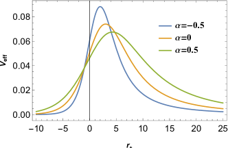
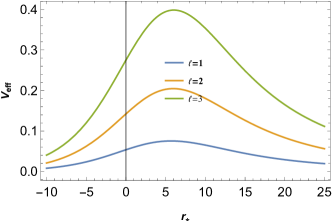
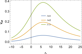
Figure 1: Variation of effective potential with respect to tortoise coordinate $r_{*}$. The upper ones are for various values of $\alpha$ with $\ell=1$ and the lower ones are for various values of angular momentum $\ell$ with $\alpha=1.0$. The left ones are for scalar perturbations and the right ones are for electromagnetic perturbations.

The LSB parameter $\alpha$ has a considerable impact on the effective potential, as seen in Fig. [1]. As a consequence, QNMs will also experience a significant impact that will be demonstrated later in this section. The LSB parameter affects both the peak as well as the position of the peak of the potential. As the parameter $\alpha$ increases, the peak of the potential moves to the right and diminishes in value.

Next, we employ the $6th$-order WKB method to obtain QNMs due to scalar and electromagnetic perturbation. To compute QNMs, the use of WKB method which was first conducted by Schutz and Will schutz . It was later extended to higher orders in the subsequent works iyer ; iyer1 ; konoplya1 ; konoplya2 . The $6th$-order WKB method yields the following expression of quasinormal frequencies:

$$\frac{\text{i}(\omega^{2}-V_{0})}{\sqrt{-2V_{0}^{{}^{\prime\prime}}}}-\sum^{6}_{\text{i}=2}\Omega_{\text{i}}=n+\frac{1}{2},$$ (9)

where $V_{0}$ and $V^{\prime\prime}_{0}$ represent respectively the height of the effective potential and the second derivative of it at its maxima with respect to the tortoise coordinate and $\Omega_{\text{i}}$ are the correction terms according to the notations followed in schutz ; iyer ; iyer1 ; konoplya1 . To illustrate the impact of the LSB parameter on the QNMs of the black hole under consideration, we tabulate numerical values of the quasinormal frequencies due to scalar and electromagnetic perturbations for various values of angular momentum $\ell$ and parameter $\alpha$. For the overtone number $n=0$, we tabulate quasinormal frequencies for scalar in Table [1], and the quasinormal frequencies for electromagnetic perturbation are tabulated in Table [2]. The error associated with the $6th$ order WKB method is also provided with the help of the equation given below:

$$\Delta_{6}=\frac{|\omega_{7}-\omega_{5}|}{2},$$ (10)

where $\omega_{5}$ and $\omega_{7}$ are quasinormal frequencies obtained using $5th$ order and $7th$ order terms respectively in the mathematical expression (series) QNMs obtained using the WKB method.

Table 1: Quasinormal frequencies for scalar perturbation with $n=0$.

$\alpha$	$\ell=1$	$\Delta_{6}$	$\ell$=2	$\Delta_{6}$	$\ell$=3	$\Delta_{6}$
-0.5	0.316497  -0.130423 i	0.00030487	0.526068  -0.129494 i	0.000033815	0.736024  -0.129291 i	$5.28627\times 10^{-6}$
-0.25	0.302284  -0.111493 i	0.000171713	0.500772  -0.110525 i	0.0000163295	0.699948  -0.110283 i	$2.54684\times 10^{-6}$
0.	0.29291  -0.0977616 i	0.0000985776	0.483642  -0.0967661 i	$8.50954\times 10^{-6}$	0.675366  -0.0965006 i	$1.33385\times 10^{-6}$
0.25	0.286619  -0.0870839 i	0.0000577862	0.471729  -0.08607 i	$4.68775\times 10^{-6}$	0.658126  -0.0857906 i	$7.35039\times 10^{-7}$
0.5	0.282529  -0.0783729 i	0.0000337063	0.463522  -0.0773494 i	$2.64843\times 10^{-6}$	0.646094  -0.0770625 i	$4.17979\times 10^{-7}$

Table 2: Quasinormal frequencies for electromagnetic perturbation with $n=0$.

$\alpha$	$\ell=1$	$\Delta_{6}$	$\ell$=2	$\Delta_{6}$	$\ell$=3	$\Delta_{6}$
-0.5	0.257511  -0.121984 i	0.000607021	0.49203  -0.126647 i	0.0000285133	0.711934  -0.127869 i	$4.47326\times 10^{-6}$
-0.25	0.252083  -0.105091 i	0.000287745	0.471644  -0.108353 i	0.0000135937	0.679313  -0.109193 i	$2.16552\times 10^{-6}$
0.	0.248191  -0.092637 i	0.000144615	0.457593  -0.0950112 i	$7.02456\times 10^{-6}$	0.656898  -0.0956171 i	$1.13678\times 10^{-6}$
0.25	0.245539  -0.0828292 i	0.0000768655	0.447725  -0.0845992 i	$3.82553\times 10^{-6}$	0.641097  -0.0850482 i	$6.27721\times 10^{-7}$
0.5	0.243917  -0.0747463 i	0.0000415175	0.440902  -0.0760844 i	$2.17153\times 10^{-6}$	0.630037  -0.0764224 i	$3.58897\times 10^{-7}$

The impact of LSB on quasinormal frequency is distinctly visible from the above tables. We can infer from Tables [1, 2] that the real part of quasinormal frequencies that corresponds to the frequency of the gravitational waves decreases with an increase in $\alpha$ for both types of perturbations. On the other hand, the imaginary part of the quasinormal frequencies show the opposite effect. This implies that the frequency of gravitational waves as well as the damping rate decreases with $\alpha$. The variation of the decay rate with the angular momentum, however, is marginal. However, the impact of $\ell$ on decay rate for scalar and electromagnetic perturbations are opposite in nature. For scalar perturbation, the decay rate decreases with $\ell$ and for electromagnetic perturbation, the decay rate increases with $\ell$. Additionally, we observe that the error follows the same pattern as followed by the decay rate or the frequency. Tables [1, 2] have shown quantitative variation of quasinormal frequencies. For completeness, we illustrate the qualitative nature of variation through a graphical presentation of quasinormal frequencies for various situations. A comparison of real and imaginary parts of quasinormal frequencies due to scalar and electromagnetic perturbations are also presented through plots.

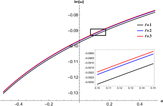
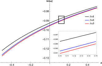
Figure 2: It gives the variation of the imaginary part of the quasinormal frequency with respect to $\alpha$ for various values of $\ell$. The left one is for the scalar field and the right one is for the electromagnetic field.

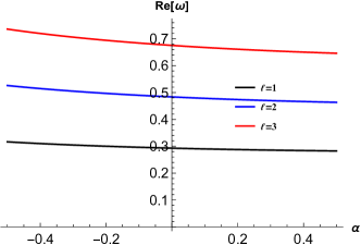
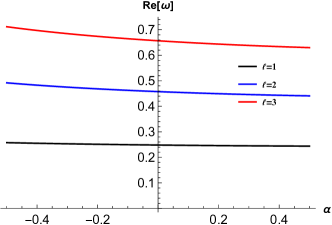
Figure 3: It gives the variation of the real part of the quasinormal frequency with respect to $\alpha$ for various values of $\ell$. The left one is for the scalar field and the right one is for the electromagnetic field.

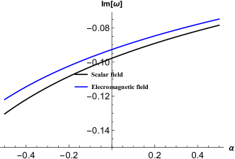
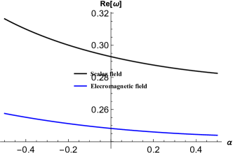
Figure 4: The Left one gives the variation of the imaginary part of the quasinormal frequency with respect to $\alpha$ for scalar and electromagnetic fields and the right one gives that for the real part. Here, we have taken $\ell=1$.

Fig. [2] and Fig. [3] reinforce what we have already known from Tables [1, 2]. Fig. [4] shows that the frequency of the gravitational wave as well as the decay rate is larger for scalar perturbation. The convergence of the WKB method for various values of $(n,\ell)$ pair is graphically illustrated below.

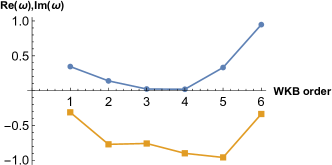
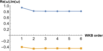
Figure 5: Variation of the real and imaginary parts of quasinormal frequencies with respect to WKB order for various values of the $(n,\ell)$ pair is shown. The left one is for the (3,0) pair and the right one is for the (2,4) pair. In each plot, the blue line is for the real part, and the orange line is for the imaginary part of the QNMs. Here, we have taken $\alpha=0.2$.

Fluctuation of quasinormal frequencies even for higher order for the pair $(3,0)$ as shown in Fig. [5] that confirms the conclusion drawn in the manuscript kd where it is observed that the WKB approximation is reliable when the angular momentum is high and the overtone number is low.

The study of the time evolution of perturbation profiles provides another avenue to observe the impact of the Lorentz violation. To this end, the time domain integration method formulated by Gundlach et al. in their article gundlach1 is employed here to numerically solve the time-dependent wave equation. We use the initial conditions $\psi(r_{*},t)=\exp\left[-\dfrac{(r_{*}-\hat{r}_{*})^{2}}{2\sigma^{2}}\right]$ and $\psi(r_{*},t)|_{t<0}=0$ with $r_{*}=5$, $\hat{r}_{*}=0.4$. While choosing the values of $\Delta t$ and $\Delta r_{*}$, we take into account the Von Neumann stability condition, $\frac{\Delta t}{\Delta r_{*}}<1$.

The dependence of the ringdown waveform on the LSB parameter $\alpha$ is graphically illustrated in the Fig. [6] and the ringdown waveforms for various values of $\ell$ are shown in the Fig. [7]. These figures indicate the effect of LSB time profiles of perturbations and confirm our conclusions drawn from Tables [1, 2].

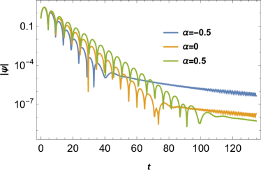
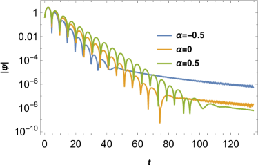
Figure 6: Time domain profile for various values of $\alpha$. The left one is for scalar perturbation and the right one is for electromagnetic perturbation. Here, we have taken $\ell=3$.

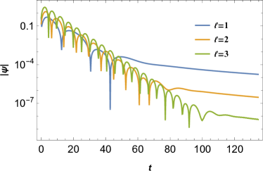
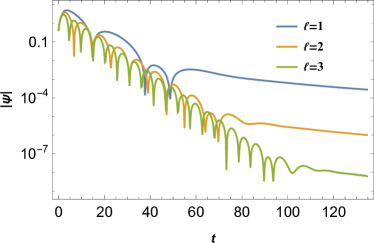
Figure 7: Time domain profile for various values of $\ell$. The left one is for scalar perturbation and the right one is for electromagnetic perturbation. Here, we have taken $\alpha=0.5$.

IV Spectrum and sparsity of Hawking radiation

Here, we investigate the effect of the LSB parameter on the spectrum and the sparsity of the Hawking radiation. For this purpose, we first need to calculate the Hawking temperature and the greybody bounds. The Hawking temperature is given by

$$T_{H}=\frac{1}{4\pi\sqrt{-g_{tt}g_{rr}}}\frac{dg_{tt}}{dr}|_{r=r_{h}},$$ (11)

where $r_{h}$ is the position of the event horizon which is $2M$ in our case. Putting metric coefficients from [2] in the above equation, we get

$$T_{H}=\frac{1}{8\pi\sqrt{\left(1-\frac{\alpha}{4}\right)^{5}\left(\frac{3\alpha}{4}+1\right)}M}.$$ (12)

The above expression reduces to that for the Schwarzschild case in the limit $\alpha\rightarrow 0$. To have a qualitative idea of the variation of the Hawking temperature with $\alpha$, we plot $T_{H}$ with respect to $\alpha$ in Fig. [8]. It shows that the Hawking temperature initially decreases with $\alpha$ reaching a minimum value at $\alpha=-0.444445$ and then starts increasing with $\alpha$.

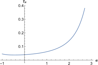
Figure 8: Variation of Hawking temperature with respect to $\alpha$.

The next ingredient required to study the spectrum and sparsity is the greybody bound given by GB ; GB1 ; GB2 ; ac2020

$$T\geq sech^{2}(\frac{1}{2\omega}\int_{-\infty}^{\infty}|V_{\text{eff}}(r_{*})|dr_{*}).$$ (13)

The analytical expression for the greybody bound of the black hole under consideration is provided in the article affine1 . Now, with the requisite information in hand, we are in a position to delve into the central topic of this section. The expression for the total power emitted by a black hole in the form of Hawking radiation is yg2017 ; fg2016

$$\frac{dE(\omega)}{dt}\equiv P_{tot}=\sum_{\ell}T(\omega)\frac{\omega}{e^{\omega/T_{H}}-1}\hat{k}\cdot\hat{n}~{}\frac{d^{3}k~{}dA}{(2\pi)^{3}},$$ (14)

where $dA$ is the surface element, $\hat{n}$ is unit normal to $dA$, and $T$ is the greybody factor given by Eq. (LABEL:gb). For massless particles $|k|=\omega$ which reduces above expression to

$$P_{tot}=\sum_{\ell}\int_{0}^{\infty}P_{\ell}\left(\omega\right)d\omega.$$ (15)

Here, $P_{\ell}$ is the power spectrum in the $\ell th$ mode given by

$$P_{\ell}\left(\omega\right)=\frac{A}{8\pi^{2}}T(\omega)\frac{\omega^{3}}{e^{\omega/T_{H}}-1}.$$ (16)

Here, $A$ is a multiple of the horizon area. We take it to be equal to the horizon area as it will not affect the qualitative result yg2017 . To study the qualitative nature of variation of the power spectrum with respect to the LSB parameter $\alpha$, we plot $P_{\ell}(\omega)$ against $\omega$ for various values of $\alpha$.

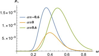
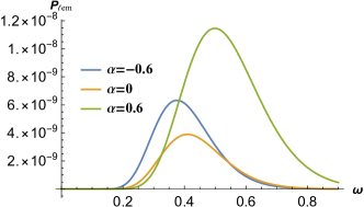
Figure 9: Power spectrum of the black hole for various values of $\alpha$. The left one is for scalar perturbation and the right one is for electromagnetic perturbation. Here, we have taken $\ell=2$.

An interesting observation we can make from Fig. [9] is that for both perturbations, $P_{\ell}(\omega)$ increases for non-zero values of the LSB parameter, whereas the peak shifts towards left for negative values of $\alpha$ and shifts towards right for positive values of $\alpha$.

The sparsity of the Hawking radiation can be quantitatively measured with the help of a dimensionless quantity $\eta$ defined by yg2017 ; fg2016 ; ac2020 ; sh2016 ; sh2015

$$\eta=\frac{\tau_{gap}}{\tau_{emission}}.$$ (17)

Here, $\tau_{gap}$ and $\tau_{emission}$ are the average time gap between two successive radiation quanta and the time taken by a radiation quantum for emission, respectively. They are defined as follows:

$$\tau_{gap}=\frac{\omega_{max}}{P_{tot}}\quad\text{and}\quad\tau_{emission}\geq\tau_{localization}=\frac{2\pi}{\omega_{max}},$$ (18)

where $\tau_{localization}$ corresponds to the time period of the emitted wave of frequency $\omega_{max}$. The significance of the quantity $\eta$ lies in the fact that it provides insight into the continuous or discontinuous nature of flow of the Hawking radiation. For $\eta\ll 1$, we have a continuous flow of radiation, whereas large values of $\eta$ signify a discontinuous flow of radiation. Tables [3, 4] provide numerical values of $\omega_{max}$, $P_{max}$, $P_{tot}$, and $\eta$ for scalar and electromagnetic perturbations, respectively. A common trend we can observe from the tables is that $P_{max}$ and $P_{\text{tot}}$ initially decreases with $\alpha$ and then starts increasing. The sparsity, on the other hand, initially increases and then decreases with an increase in the LSB parameter. It clearly shows the significant impact of the Lorentz violation effect on Hawking radiation.

Table 3: Numerical values of $\omega_{max}$, $P_{max}$, $P_{tot}$, and $\eta$ for scalar perturbation for various values of $\alpha$ for $\ell=1$ mode.

$\alpha$	-1.	-0.5	0.	0.5	1.	1.5	2.0	2.5	3.0
$\omega_{max}$	0.171431	0.201873	0.235445	0.286453	0.365994	0.497487	0.735941	1.24294	2.69832
$P_{max}$	0.00005	5.49255$\times 10^{-6}$	3.42190$\times 10^{-6}$	4.90236$\times 10^{-6}$	0.00001	0.00005	0.00038	0.00513	0.17181
$P_{\text{tot}}$	9.6149$\times 10^{-6}$	9.81224$\times 10^{-7}$	6.71889$\times 10^{-7}$	1.15588$\times 10^{-6}$	3.84193$\times 10^{-6}$	2.30024$\times 10^{-5}$	2.57345$\times 10^{-4}$	6.32755$\times 10^{-3}$	5.32169$\times 10^{-1}$
$\eta$	486.468	6610.08	13131.1	11298.3	5549.05	1712.42	334.958	38.8585	2.1775

Table 4: Values of $\omega_{max}$, $P_{max}$, $P_{tot}$, and $\eta$ for electromagnetic perturbation for various values of $\alpha$ for $\ell=1$ mode.

$\alpha$	-1.	-0.5	0.	0.5	1.	1.5	2.0	2.5	3.0
$\omega_{\max}$	0.262231	0.243064	0.263861	0.308454	0.385231	0.514836	0.752186	1.25849	2.71274
$P_{\max}$	6.28359$\times 10^{-6}$	1.37354$\times 10^{-6}$	1.33432$\times 10^{-6}$	2.60945$\times 10^{-6}$	8.39995$\times 10^{-6}$	0.00004	0.00034	0.00484	0.16908
$P_{tot}$	1.39766$\times 10^{-6}$	2.63489$\times 10^{-7}$	2.74252$\times 10^{-7}$	6.34356$\times 10^{-7}$	2.61403$\times 10^{-6}$	1.82744$\times 10^{-5}$	2.27702$\times 10^{-4}$	5.99975$\times 10^{-3}$	5.2402$\times 10^{-1}$
$\eta$	7830.45	35686.1	40403.7	23870.9	9035.49	2308.42	395.461	42.013	2.23506

V Hawking evaporation and the lifetime of LSB black holes

Black holes emit radiation that causes a reduction in the black hole mass and gives rise to Hawking evaporation. We, in this section, intend to obtain the ’lifetime’, $\tau$, of LSB black holes. With the help of the Stefan-Boltzmann radiation law, the rate of energy loss is given by

$$\frac{dM}{dt}=-\gamma M^{2}T_{H}^{4},$$ (19)

where $\gamma$ is a constant that is related to the greybody factor and the radiation constant, $T_{H}$ is the Hawking temperature given by Eq. [12] ong . The above equation, with the help of Eq. [12], yields

$$\frac{dM}{dt}=-\frac{\gamma}{4096\pi^{4}\left(1-\frac{\alpha}{4}\right)^{10}\left(\frac{3\alpha}{4}+1\right)^{2}M^{2}}.$$ (20)

To obtain the lifetime of LSB black holes, we integrate the above equation from the initial mass $M_{i}$ to $0$. That produces the result:

$$\tau=\frac{4096\pi^{4}\left(1-\frac{\alpha}{4}\right)^{10}\left(\frac{3\alpha}{4}+1\right)^{2}M_{i}^{3}}{3\gamma}.$$ (21)

The above result clearly exhibits the dependence of $\tau$ on the LSB parameter $\alpha$. To analyze the qualitative variation of $\tau$ with $\alpha$, we plot $\tau$ versus $\alpha$ with $M_{i}=\gamma=1$.

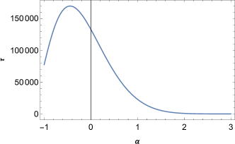
Figure 10: Variation of $\tau$ with respect to $\alpha$.

Figure [10] shows us that a black hole’s lifetime first rises with $\alpha$, reaches its highest value at $\alpha=-0.444444$, and then falls. The maximum value of the Hawking temperature is found in proximity to the lowest value.

VI Discussion and conclusions

Using the static solution provided in AFFINE from the metric-affine bumblebee model, in this work, we have computed the correction owing to the LSB effects on the QNMs, ringdown waveforms, Hawking radiation spectra, the sparsity of Hawking radiation, and the lifetimes of black holes presenting a variety of graphs and tables. The impact of the LSB on these black hole-related physical properties have been thoroughly examined.

To illustrate the impact of LSB on QNMs, we have employed the $6th$-order WKB method. To start with, we provide numerical values for QNMs for scalar and electromagnetic perturbations in tabular form, then illustrate graphically how the real and imaginary parts of QNMs vary with respect to the LSB parameter $\alpha$. Errors associated with our numerical calculations are also provided. Additionally, we compare the decay rate and the frequency of gravitational waves of scalar and electromagnetic perturbations. Our investigation reveals that the decay rate associated with the imaginary part of the QNMs and the frequency of gravitational waves corresponding to the real part of the QNMs initially decreases with the increase in the LSB parameter $\alpha$, and then starts increasing. Note that the frequency of the gravitational wave and decay rate are found to be more sensitive to negative values of the LSB parameter $\alpha$ than to its positive values (see Fig. [4]). As a result, the LSB is expected to be crucially important for maintaining the stability of the system if receives perturbation from either a scalar or electromagnetic field. It is expected to hold for other types of perturbation. We also observe that the real part of QNMs increases with the angular momentum $\ell$, but the impact of $\ell$ on the decay rate is marginal. The comparison between scalar and electromagnetic perturbations reveals that both the decay rate and the frequency of gravitational waves are a little larger for the scalar perturbation in comparison to the electromagnetic perturbation. We have also studied the evolution of perturbation profiles, which confirm the conclusions we have already drawn from qualitative and quantitative studies. In Fig. [5], we illustrate the convergence of the WKB. method for various $(n,\ell)$ pairs. We observe that, for $n<\ell$, QNMs fluctuate even for higher order.

We then delve into the study of the Hawking spectrum and its sparsity. In order to accomplish this, we first determine the Hawking temperature and the greybody bounds for the black hole under consideration. The variation of the Hawking temperature is shown in Fig. [8]. The plot reveals that the Hawking temperature initially decreases to a minimum value at$\alpha=-0.444445$ and then increases with $\alpha$. With the help of the Hawking temperature and the graybody bounds, we study the variation of the power spectrum $P_{\ell}(\omega)$ with respect to the LSB parameter $\alpha$. We can infer from Fig. [9] that for both types of perturbation $P_{\ell}(\omega)$ increases for non-zero values of the LSB parameter, whereas the peak shifts towards the left for negative values of $\alpha$, and for positive values of $\alpha$, it shifts towards the right. We then tabulate. numerical values of $\omega_{max}$, $P_{max}$, $P_{tot}$, and $\eta$ for both scalar and electromagnetic perturbations. The findings indicate that with the increase in$\alpha$, there is an initial decline of $P_{max}$, and $P_{\text{tot}}$, followed by an enhancement. On the other hand, the sparsity, i.e., the time gap between successive radiation quanta, initially increases with $\alpha$ and then falls off. Besides, our study on Hawking evaporation shows that the Lorentz symmetry violation has a significant impact on the lifetime of black holes associated with the metric-affine bumblebee model.

In this endeavor, we provide our findings that demonstrate the significant influence of the LSB on several observables, such as QNMs, Hawking temperature, sparsity of Hawking radiation, temporal evaluation of perturbation profiles, and lifetime of black hole. Our knowledge of modified theories of gravity and its astrophysical ramifications will be improved by these findings. Nevertheless, the experiment will establish to what extent a modified theory of gravity is applicable. Experiments in this energy regime are, however, sparse. Precise standardization of this type of theory is therefore currently outside the purview. In this context, we must mention that in AFFINE , we found an effort to constrain the LSB parameter using low-energy experimental observation.

References

- (1) T. Regge, J. A. Wheeler, Stability of a Schwarzschild singularity Phys. Rev. 108 1063 (1957)
- (2) H. W. Press, Long wave trains of gravitational waves from a vibrating black hole, Astrophys. J 170, L105-L108 (1971)
- (3) V. C. Vishveshwara, Scattering of gravitational radiation by a Schwarzschild black-hole, Nature. 227:936-938 (1970)
- (4) K. D. Kokkotas, B. G. Schmidt, Living Rev. Rel. 2, 2 (1999), arXiv:gr-qc/9909058.
- (5) Hans-Peter Nollert, Class. Quant. Grav. 16, R159 (1999).
- (6) R. A. Konoplya, A. Zhidenko, Rev. Mod. Phys. 83, 793 (2011), arXiv:1102.4014 [gr-qc].
- (7) E. Berti, V. Cardoso, A. O. Starinets, Class. Quant. Grav. 26, 163001 (2009), arXiv:0905.2975 [gr-qc].
- (8) L. Barack et al., Class. Quant. Grav. 36, 143001 (2019), arXiv:1806.05195 [gr-qc].
- (9) K. Akiyama et al. (Event Horizon Telescope), Astrophys. J. Lett. 930, L17 (2022).
- (10) C. Goddi et al., Int. J. Mod. Phys. D 26, 1730001 (2016), arXiv:1606.08879 [astro-ph.HE].
- (11) R. Konoplya, A. Zhidenko, Phys. Lett. B 756, 350 (2016), arXiv:1602.04738 [gr-qc].
- (12) G.T. Zatsepin, V.A. Kuzmin, Upper limit of the spectrum of cosmic rays, JETP Lett. 4, 78 (1966).
- (13) M. Takeda et al., Extension of the cosmic ray energy spectrum beyond the predicted Greisen-Zatsepin-Kuz’min cutoff, Phys. Rev. Lett. 81, 1163 (1998); arXiv:astro-ph/9807193.
- (14) V.A. Kostelecky and S. Samuel, Photon and graviton masses in string theories, Phys. Rev. Lett. 66, 1811 (1991).
- (15) V.A. Kostelecky, R. Potting, CPT, strings, and meson factories, Phys. Rev. D 51, 3923 (1995).
- (16) D. Colladay, V.A. Kostelecky, CPT violation and the standard model, Phys. Rev. D 55, 6760 (1997)
- (17) V.A. Kostelecky, S. Samuel, Spontaneous breaking of Lorentz symmetry in string theory, Phys. Rev. D 39, 683 (1989).
- (18) V.A. Kostelecky, S. Samuel, Gravitational Phenomenology in Higher Dimensional Theories and Strings, Phys. Rev. D 40, 1886 (1989).
- (19) R. Bluhm, V.A. Kostelecky, Spontaneous Lorentz violation, Nambu-Goldstone modes, and gravity, Phys. Rev. D 71, 065008 (2005); arXiv:hep-th/0412320.
- (20) O. Bertolami, J. Paramos, The Flight of the bumblebee: Vacuum solutions of a gravity model with vector-induced spontaneous Lorentz symmetry breaking, Phys. Rev. D 72, 044001 (2005); arXiv:hep-th/0504215.
- (21) Q.G. Bailey, V.A. Kostelecky, Signals for Lorentz violation in post-Newtonian gravity, Phys. Rev. D 74, 045001 (2006); arXiv:gr-qc/0603030.
- (22) R. Bluhm, N.L. Gagne, R. Potting, A. Vrublevskis, Constraints and Stability in Vector Theories with Spontaneous Lorentz Violation, Phys. Rev. D 77, 125007 (2008); Erratum ibid. D79 029902 (2009); arXiv:0802.4071 [hep-th].
- (23) V.A. Kostelecky, J. Tasson, Prospects for Large Relativity Violations in Matter-Gravity Couplings, Phys. Rev. Lett. 102, 010402 (2009); arXiv:0810.1459 [gr-qc].
- (24) M.D. Seifert, Generalized bumblebee models and Lorentz-violating electrodynamics, Phys. Rev. D 81, 065010 (2010); arXiv:0909.3118 [hep-ph].
- (25) R.V. Maluf, C.A.S. Almeida, R. Casana, and M. Ferreira, Einstein-Hilbert graviton modes modified by the Lorentz violating bumblebee Field, Phys. Rev. D 90, 025007 (2014); arXiv:1402.3554 [hep-th].
- (26) J. Paramos and G. Guiomar, Astrophysical Constraints on the Bumblebee Model, Phys. Rev. D 90, 082002 (2014); arXiv:1409.2022 [astro-ph].
- (27) C.A. Escobar and A. Martn-Ruiz, Equivalence between bumblebee models and electrodynamics in a nonlinear gauge, Phys. Rev. D 95, 095006 (2017); arXiv:1703.01171 [hep-th].
- (28) D. Capelo and J. Paramos, Cosmological implications of Bumblebee vector models, Phys. Rev. D 91, 104007 (2015); arXiv:1501.07685 [gr-qc].
- (29) W. Liu, X. Fang, J. Jing, J. Wang, Exact Kerr-like solution and its shadow in a gravity model with spontaneous Lorentz symmetry breaking, Eur. Phys. J. C 83, 83 (2023); arXiv:2211.03156 [gr-qc].
- (30) J.F. Assunao, T. Mariz, J.R. Nascimento, A.Y. Petrov, Dynamical Lorentz symmetry breaking in a tensor bumblebee model, Phys. Rev. D 100, 085009 (2019); arXiv:1902.10592 [hep-th].
- (31) A. Uniyal, S. Kanzi, I. Sakall, Greybody factors of bosons and fermions emitted from higher dimensional dS/AdS black holes in Einstein-bumblebee gravity theory, Eur. Phys. J. C 83 668 (2023) arXiv:2207.10122 [hep-th].
- (32) M. Khodadi and M. Schreck, Hubble tension as a guide for refining the early Universe: Cosmologies with explicit local Lorentz and diffeomorphism violation, Phys. Dark Universe 39, 101170 (2023).
- (33) C.M. Reyes, M. Schreck, A. Soto, Cosmology in the presence of diffeomorphism-violating, nondynamical background fields, Phys. Rev. D 106, 023524 (2022); arXiv:2205.06329 [gr-qc].
- (34) R. Casana, A. Cavalcante, F.P. Poulis, E.B. Santos, Exact Schwarzschild-like solution in a bumblebee gravity model, Phys. Rev. D 97, 104001 (2018); arXiv:1711.02273 [gr-qc].
- (35) A. Ovgun, K. Jusufi, I. Sakalli, Gravitational Lensing Under the Effect of Weyl and Bumblebee Gravities: Applications of Gauss-Bonnet Theorem, Ann. Phys. 399, 193 (2018); arXiv:1805.09431 [gr-qc].
- (36) R. Oliveira, D.M. Dantas, C.A.S. Almeida, Quasinormal frequencies for a black hole in a bumblebee gravity, EPL 135, 10003 (2021); arXiv:2105.07956 [gr-qc].
- (37) I. Gullu A. Ovgun, Schwarzschild-like black hole with a topological defect in bumblebee gravity, Ann. Phys. 436, 168721 (2022); arXiv:2012.02611 [gr-qc].
- (38) R.V. Maluf, J. C. S. Neves, Black holes with a cosmological constant in bumblebee gravity, Phys. Rev. D 103, 044002 (2021).
- (39) C. Ding, X. Chen, and X. Fu, Einstein-Gauss-Bonnet gravity coupled to bumblebee field in four-dimensional spacetime, Nucl. Phys. B 975, 115688 (2022); arXiv:2102.13335 [gr-qc].
- (40) A. Ovgun, K. Jusufi, I. Sakall, Exact traversable wormhole solution in bumblebee gravity, Phys. Rev. D 99, 024042 (2019); arXiv:1804.09911 [gr-qc].
- (41) S. Kanzi and I. Sakalli, GUP Modified Hawking Radiation in Bumblebee Gravity, Nucl. Phys. B 946, 114703 (2019); arXiv:1905.00477 [hep-th].
- (42) C. Ding, C. Liu, R. Casana, A. Cavalcante, Exact Kerr-like solution and its shadow in a gravity model with spontaneous Lorentz symmetry breaking, Eur. Phys. J. C 80, 178 (2020); arXiv:1910.02674 [gr-qc].
- (43) H. Wang, S. Wei, Shadow cast by Kerr-like black hole in the presence of plasma in Einstein-bumblebee gravity, Eur. Phys. J. Plus 137, 571 (2022); arXiv:2106.14602 [gr-qc].
- (44) C. Liu, C. Ding, J. Jing, Thin accretion disk around a rotating Kerr-like black hole in Einstein-bumblebee gravity model, arXiv:1910.13259 [gr-qc].
- (45) R. Jiang, R. Lin, X. Zhai, Superradiant instability of the Kerr-like black hole in Einstein-bumblebee gravity, Phys. Rev. D 104, 124004 (2021); arXiv:2108.04702 [gr-qc].
- (46) Z. Li and A. Ovgun, Finite-distance gravitational deflection of massive particles by a Kerr-like black hole in the bumblebee gravity model, Phys. Rev. D 101, 024040 (2020); arXiv:2001.02074 [gr-qc].
- (47) S.K. Jha, A. Rahaman, Bumblebee gravity with a Kerr-Sen-like solution and its Shadow, Eur. Phys. J. C 81, 345 (2021); arXiv:2011.14916 [gr-qc].
- (48) S.E. Motta, T.M. Belloni, L. Stella, T. Muoz-Darias, R. Fender, Precise mass and spin measurements for a stellar-mass black hole through X-ray timing: the case of GRO J1655-40, MNRAS 437 2554 (2014), arXiv:1309.3652 [astro-ph].
- (49) J.A. Orosz, J.F. Steiner, J.E. McClintock, M.A.P. Torres, R.A. Remillard, C.D. Bailyn, and J.M. Miller, An Improved Dynamical Model for the Microquasar XTE J1550-564, Astrophys. J. 730, 75 (2011); arXiv:1101.2499 [astro-ph].
- (50) M.J. Reid, J.E. McClintock, J.F. Steiner, D. Steeghs, R.A. Remillard, V. Dhawan, and R. Narayan, A Parallax Distance to the Microquasar GRS 1915+105 and a Revised Estimate of its Black Hole Mass, Astrophys. J. 796, 2 (2014); arXiv:1409.2453 [astro-ph].
- (51) A. A. Araujo Filho, J. R. Nascimento, A. Y. Petrov, P. J. Porfirio: Vacuum solution within a metric-affine bumblebee gravity Phys. Rev. D 108, 085010 (2023),arXiv:2211.11821[gr-qc]
- (52) F. B. Schutz M. C. Will Black hole normal modeds: A schematic approach Astrophys. J. Lett. 291 L33-L36 (1985)
- (53) S. Iyer M. C. Will Black Hole Normal Modes: A WKB Approach. 1. Foundations and Application of a Higher Order WKB Analysis of Potential Barrier Scattering Phys. Rev. D 35 3621 (1987)
- (54) S. Iyer Black hole normal modeds: A WKB aproach 2. Schwarzschild black holes Phys. Rev. D 35 3632 (1987)
- (55) R. Konoplya Quasinormal behavior of the d-dimensional Schwarzschild black hole and higher order WKB approach Phys. Rev. D68 024018 (2003)
- (56) R. A. Konoplya, A. Zhidenko, A. F. Zinhailo, Class. Quantum Grav. 36: 155002 (2019) [arXiv:1904.10333].
- (57) C. Gundlach, H. R. Price, J. Pullin Late time behavior of stellar collapse and explosions: 2. Nonlinear evolution Phys. Rev. D 49 890-899 (1994)
- (58) K. Destounis, R. P. Macedo, E. Berti, V. Cardoso, J. L. Jaramillo, Pseudospectrum of Reissner-Nordstrrm black holes: quasinormal mode instability and universality, Phys. Rev. D 104, 084091 (2021) arXiv:2107.09673[gr-qc] .
- (59) S. W. Hawking, Commun. Math. Phys. 43, 199 (1975), [Erratum: Commun.Math.Phys. 46, 206 (1976)]
- (60) Black hole thermodynamics, Physics Today J. D. Bekenstein,Physics Today 33 (1), 24 (1980)
- (61) J M Stewart Classical and Quantum black holes: Classical and Quantum Gravity 17 513 (2000)
- (62) M. Visser, Some general bounds for one-dimensional scattering, Phys. Rev. A 59, 427 (1999).
- (63) P. Boonserm, M. Visser,Bounding the Bogoliubov coefficients Annls. Phys. 323, 2779 (2008).
- (64) P. Boonserm, Rigorous bounds on Transmission, Reflection, and Bogoliubov coefficients Ph.D. thesis, Victoria Univ. Wellington (2009) arXiv:0907.0045 [math-ph].
- (65) Probing Schwarzschild-like Black Holes in Metric-Affine Bumblebee Gravity with Accretion Disk, Deflection Angle, Greybody Bounds, and Neutrino Propagation: Gaetano Lambiase et al. [arXiv:2309.13594 [gr-qc]]
- (66) Y.-G. Miao, Z.-M. Xu, Hawking Radiation of Five-Dimensional Charged Black Holes with Scalar Fields, Phys. Lett. B 772, 542 (2017).
- (67) F. Gray, S. Schuster, A. Van-Brunt, M. Visser, The Hawking Cascade from a Black Hole Is Extremely Sparse, Class. Quantum Grav. 33, 115003 (2016).
- (68) A. Chowdhury, N. Banerjee, Greybody Factor and Sparsity of Hawking Radiation from a Charged Spherical Black Hole with Scalar Hair, Phys. Lett. B 805, 135417 (2020).
- (69) S. Hod, The Hawking Cascades of Gravitons from Higher-Dimensional Schwarzschild Black Holes, Phys. Lett. B 756, 133 (2016) [arXiv:1605.08440].
- (70) S. Hod, The Hawking Evaporation Process of Rapidly-Rotating Black Holes: An Almost Continuous Cascade of Gravitons, Eur. Phys. J. C 75, 329 (2015) [arXiv:1506.05457].
- (71) Y.C. Ong, An effective black hole remnant via infinite evaporation time due to generalized uncertainty principle, J. High Energ. Phys.,10 195 (2018)
- (72) V. A. Kostelecky, Gravity, Lorentz Violation, and the Standard Model, Phys. Rev. D 69 105009 (2004) arXiv:hep-th/0312310 [hep-th]
- (73) J. R. Nascimento, A. Y. Petrov, P. J. Porfirio, Induced gravitational topological term and the Einstein-Cartan modified theory, Phys. Rev. D 105, 044053 (2022) [arXiv:2108.05705 [gr-qc]].
- (74) D. Bao, S.-S. Chern, Z. Shen, An Introduction to Riemann-Finsler Geometry (Springer, New York, 2000).
- (75) J. Foster, R. Lehnert, Classical-physics applications for Finsler b space, Phys. Lett. B 746, 164 (2015), arXiv:1504.07935 [physics.class-ph].
- (76) B. R. Edwards, V. A. Kostelecky, Phys. Lett. B 786, 319 (2018), arXiv:1809.05535 [hep-th].
- (77) M. Schreck, Classical kinematics and Finsler structures for nonminimal Lorentz-violating fermions, Eur. Phys. J. C 75, 187 (2015), arXiv:1405.5518 [hep-th].
- (78) D. Colladay and P. McDonald, Singular Lorentz-Violating Lagrangians and Associated Finsler Structures, Phys. Rev. D 92, 085031 (2015), arXiv:1507.01018 [hep-ph].
- (79) M. Schreck, Classical Lagrangians and Finsler structures for the nonminimal fermion sector of the Standard-Model Extension, Phys. Rev. D 93, 105017 (2016), arXiv:1512.04299 [hep-th].
- (80) D. M. Ghilencea, Eur. Phys. J. C 80, 1147 (2020) arXiv:2003.08516 [hep-th]
- (81) D. M. Ghilencea,Palatini quadratic gravity: spontaneous breaking of gauged scale symmetry and inflation, Eur. Phys. J. C 81, 518 (2021) [arXiv:2007.14733 [hep-th]].
- (82) A. Delhom, J. Nascimento, G. J. Olmo, A. Y. Petrov, P. J. Porfirio, Metric-affine bumblebee gravity: classical aspects, Eur.Phys.J. C 81 (2021), 287 arXiv:1911.11605 [hep-th]
- (83) A. Delhom, J. Nascimento, G. J. Olmo, A. Y. Petrov, P. Porfirio, Radiative corrections in metric-affine bumblebee model, Phys. Lett. B 826 (2022) 136932, arXiv: 2010.06391 [hep-th].
- (84) A. Delhom, T. Mariz, J. R. Nascimento, G. J. Olmo, A. Y. Petrov, P. J. Porfirio, Spontaneous Lorentz symmetry breaking and one-loop effective action in the metric-affine bumblebee gravity, JCAP 07 (2022) 018 [arXiv:2202.11613 [hep-th]].
- (85) F. Pretorius, Evolution of binary black-hole spacetimes, Phys. Rev. Letts, 95, 121101 (2005)
- (86) J. R. Hurley, C. A. Tout, O. R. Pols, Evolution of binary stars and the effect of tides on binary populations, MNRAS 329, 897 (2002), arXiv:astro-ph/0201220
- (87) K. Yakut, P. P. Eggleton, Evolution of close binary systems, The Astrophysical Journal, 629, 1055 (2005)
- (88) E. V. D. Heuvel, Compact stars and the evolution of binary systems, Bull. Astr. Soc. India 39, 1-20 (2011)
- (89) K. Riles, Recent searches for continuous gravitational waves, Mod. Phys. Letts. A 32, 17300355 (2017) arXiv:1712.05897
- (90) R. Konoplya, A. Zhidenko, Quasinormal modes of black holes: From astrophysics to string theory, Revs. Mod. Phys, 83 793, (2011), arXiv:1102.4014 [gr-qc].
- (91) N. Heidari, H. Hassanabadi, J. Kurouz, S. Zare, P. Porfirio, Gravitational signatures of a non-commutative stable black hole, arXiv:2305.06838, 2023.