Kerr black hole shadows from the axion-photon coupling

Abstract

Abstract

We have investigated the motion for photons in the Kerr black hole spacetime under the axion-photon coupling. The birefringence phenomena arising from the axion-photon coupling can be negligible in the weak coupling approximation because the leading-order contributions to the equations of motion come from the square term of the coupling parameter. We find that the coupling parameter makes the size of shadows slightly increase for arbitrary spin parameter. For the rapid rotating black hole case with a larger coupling, we find that there exist a “pedicel”-like structure appeared in the left of the “D”-type like shadows. Comparing the shadow size of the Kerr black hole with the shadow size of the Sgr A* and M87* black holes, we find that there is room for such a theoretical model of the axion-photon coupling.

I Introduction

The images of the supermassive black holes M87* fbhs1 ; fbhs6 ; fbhs12 ; fbhs13 and Sgr A* fbhs1222 ; fbhs17 open a new window to test gravity in strong field regimes. Meanwhile, they also provide a powerful way to probe electromagnetic interactions, matter distributions and accretion processes near black holes kerr1 ; kerr2 ; bhs0 ; bhs1 ; bhs2 ; bhs3 ; bhsp1 ; swo11 ; Vagnozzi ; min22 . The main components in the black hole’s image is the shadow, which is caused by light rays that fall into an outer event horizon. In general, the black hole shadow depends on the parameters of background black hole, the propagation of light ray and the position of observer. Recent studies also show that the some interactions between electromagnetic and gravitational fields leads to birefringence of photons in spacetimes, which result in double shadows for a single black hole qed1 ; qed2 ; qed3 ; weyl6 ; weyl7 ; weyl6s . These interesting features have triggered the further study of black hole shadows under interactions between electromagnetic and other fields. A phenomenological coupling between a photon and a generic vector field is also introduced to study black hole shadow epb , which shows that the black hole shadow in edge-on view has different appearances for different frequencies of the observed light.

Dark matter is widely believed to be the dominant gravitationally attractive component in the Universe although its nature is still unclear. One of the most interesting candidates for dark matter is axion, which is hypothetical pseudoscalar particle initially introduced by Peccei and Quinn cpqus to solve the strong charge-conjugation and parity problem in quantum chromodynamics. Interestingly, axion is also furthermore generically predicted in string theory Arvanitaki ; Witten ; Marsh . One of the important properties of axion is that it interacts with photon through the coupling, which leads to an interesting conversion from photons into axions and vice versa in the presence of a magnetic field Maiani ; Raffelt . Such axion-photon conversion is also regarded as basic principle Sikivie ; Irastorza to experimentally detect Solar axions Anastassopoulos ; Armengaud ; Banerjee and axion dark matter Asztalos . Moreover, to account for the recent detections of high-energy gamma ray photons from extragalactic sources, some suggestions Mirizzi ; Meyer based on the axion-photon conversion are introduced because the conversion can prevent the high-energy photons from being annihilated through electron-positron pair production in their propagations. Recent investigations Yanagida ; Mirizzi1 ; Tashiro show that the resonant axion-photon conversion inside the cluster’s magnetic field could distort the black-body spectrum of the cosmic microwave background.

As a coupling between matter and electromagnetic fields, the axion-photon coupling also results in the photon birefringence as photon crosses over axion matter. The birefringence effects of the polarization photons have been used to analyze the axion dark matter distribution near M87* black hole tomoch and in the protoplanetary disk around a young star Fujita . The axion-induced birefringence effect gives arise to the unique polarimetric structure Alexander and the electric vector position angle oscillation of linearly polarized photons Yifan . Such oscillation has been applied to constrain region of the axion mass and axion-photon coupling parameter space together with the observation data from Event Horizon Telescope Yifan . Moreover, the conversion of photons into axions leads to a dimming of the photon ring around the black hole shadow Kimihiro . The photon scattering from the background magnetic field with axions is also found to generate a significant circular polarization around the horizon of supermassive black hole Soroush and in blazars Run . The polarization-dependent bending that a ray of light experiences by traveling through an axion cloud is studied in the background of a Kerr black hole Plascencia . All above literature is focused on analyzing effects of the axion-photon coupling on the brightness and polarization patterns of surrounding emissions region in black hole images. However, it is still an open issue how the axion-photon coupling affect black hole shadows. In this paper, we start from the modified Maxwell equation and make use of the geometric optics approximation to obtain the equation of motion for the photon coupling to an axion field. Then, we probe the effects of axion-photon coupling on the shadow of a rotating black hole.

The paper is organized as follows: In Sec.II, we firstly present equation of motion for photons interacted with axion-like particle in the Kerr black hole spacetime and obtain two kind of solutions of polarized photon motions. In Sec.III, we present numerically Kerr black hole shadow under the axion-photon coupling and probe its effects on the shadow. Finally, we end the paper with a summary.

II Equation of motion for the photons coupling axion-like particles in a Kerr black hole spacetime

We firstly present the equations of motions for photons interacted with axion-like particles in a Kerr black hole spacetime by the geometric optics approximation weyl0 ; Daniels ; Caip ; Cho1 ; Lorenci . In the curved spacetime, the action contained the coupling between photon and axion-like particle can be expressed as cpqus ; Maiani ; Raffelt ; Sikivie ; Irastorza

$$S=\int d^{4}x\sqrt{-g}\bigg{[}\frac{R}{16\pi G}+\frac{1}{2}\partial_{\mu}\phi\partial^{\mu}\phi-\frac{1}{4}\bigg{(}F_{\mu\nu}F^{\mu\nu}-\alpha\phi F_{\mu\nu}\tilde{F}^{\mu\nu}\bigg{)}\bigg{]},$$ (1)

where $\phi$ denotes the axion-like field and $\tilde{F}^{\mu\nu}=\epsilon^{\mu\nu\rho\sigma}F_{\rho\sigma}/2$ is the dual of the electromagnetic field strength tensor. $\epsilon^{\mu\nu\rho\sigma}$ is the Levi-Civita tensor and $\alpha$ denotes the axion-photon coupling constant. Generally, the axion-like field $\phi$ is dynamical. Here, we assume it as a function of a radial and polar angle coordinate $\phi=\phi(r,\theta)$ for the sake of simplicity. Therefore, the coupling between photon and axion-like particle modifies Maxwell equation as

$$\nabla_{\mu}F^{\mu\nu}-2\alpha\phi_{\mu}\epsilon^{\mu\nu\rho\sigma}F_{\rho\sigma}=0,$$ (2)

where $\phi_{\mu}\equiv\partial_{\mu}\phi$. Using the geometric optics approximation weyl0 ; Daniels ; Caip ; Cho1 ; Lorenci , we can get equation of motions for coupled photons from the modified Maxwell equation (2). In this approximation, the wavelengths of photons are assumed to be much smaller than a typical curvature scale, but be larger than the electron Compton wavelength. Then, the electromagnetic tensor $F_{\mu\nu}$ can be rewritten as a simpler form

$$F_{\mu\nu}=f_{\mu\nu}e^{i\theta},$$ (3)

with a slowly varying amplitude $f_{\mu\nu}$ and a rapidly varying phase $\theta$. Comparing with the wave vector $k_{\mu}=\partial_{\mu}\theta$, one can find that the derivative term $f_{\mu\nu;\lambda}$ can be neglected since it is not dominated in this case. Making use of the Bianchi identity

$$D_{\lambda}F_{\mu\nu}+D_{\mu}F_{\nu\lambda}+D_{\nu}F_{\lambda\mu}=0,$$ (4)

it is easy to obtain that the form of the amplitude $f_{\mu\nu}$ must be

$$f_{\mu\nu}=k_{\mu}a_{\nu}-k_{\nu}a_{\mu}.$$ (5)

Here the polarization vector $a_{\mu}$ is orthogonal to the wave vector $k_{\mu}$, i.e., $k_{\mu}a^{\mu}=0$. Inserting Eqs.(3) and (5) into Eq. (2), we can obtain the modified equation of motions for photons under the axion-photon coupling

$$k_{\mu}k^{\mu}a^{\nu}-i4\alpha\phi_{\mu}\epsilon^{\mu\nu\rho\sigma}k_{\sigma}a_{\rho}=0,$$ (6)

which means that the coupling will change the propagation of photons in background spacetimes.

With the standard Boyer-Lindquist coordinates, the metric of a Kerr black hole can be expressed as

$$ds^{2} = -\rho^{2}\frac{\Delta}{\Sigma^{2}}dt^{2}+\frac{\rho^{2}}{\Delta}dr^{2}+\rho^{2}d\theta^{2}+\frac{\Sigma^{2}}{\rho^{2}}\sin^{2}{\theta}(d\phi-\omega dt)^{2},$$ (7)

with

$$\omega = \frac{2aMr}{\Sigma^{2}},\;\;\;\;\;\;\;\;\;\;\;\;\;\;\;\;\;\;\;\;\;\;\;\;\;\;\;\;\;\rho^{2}=r^{2}+a^{2}\cos^{2}\theta,$$

$$\Delta = r^{2}-2Mr+a^{2},\;\;\;\;\;\;\;\;\;\;\;\;\;\;\;\;\Sigma^{2}=(r^{2}+a^{2})^{2}-a^{2}\sin^{2}\theta\Delta.$$ (8)

Here the parameters $M$ and $a$ denote the mass and the spin parameter of the black hole, respectively. For the Kerr black hole spacetime, it is convenient to build a local set of orthonormal frames by introducing vierbein fields $e^{a}_{\mu}$ obeyed the condition

$$g_{\mu\nu}=\eta_{ab}e^{a}_{\mu}e^{b}_{\nu},$$ (9)

where $\eta_{ab}$ denotes the Minkowski metric. The forms of the vierbein fields $e^{a}_{\mu}$ and their inverse $e_{a}^{\mu}$ can be respectively expressed as

$$e^{a}_{\mu}=\left(\begin{array}[]{cccc}\rho\frac{\sqrt{\Delta}}{\Sigma}&0&0&-\frac{\omega\Sigma}{\rho}\sin\theta\\ 0&\frac{\rho}{\sqrt{\Delta}}&0&0\\ 0&0&\rho&0\\ 0&0&0&\frac{\Sigma}{\rho}\sin\theta\end{array}\right),$$ (14)

and

$$e_{a}^{\mu}=\left(\begin{array}[]{cccc}\frac{\Sigma}{\rho\sqrt{\Delta}}&0&0&0\\ 0&\frac{\sqrt{\Delta}}{\rho}&0&0\\ 0&0&\frac{1}{\rho}&0\\ \frac{\omega\Sigma}{\rho\sqrt{\Delta}}&0&0&\frac{\rho}{\Sigma\sin\theta}\end{array}\right).$$ (19)

Making use of the relationship $a^{\mu}k_{\mu}=0$, one can find that the equation of motion of the photon coupling with axion can be simplified as a set of equations for three independent polarisation components $a^{r}$, $a^{\theta}$, and $a^{\phi}$,

$$\bigg{(}\begin{array}[]{ccc}K_{11}&K_{12}&K_{13}\\ K_{21}&K_{22}&K_{23}\\ K_{31}&K_{32}&K_{33}\end{array}\bigg{)}\bigg{(}\begin{array}[]{c}a^{r}\\ a^{\theta}\\ a^{\phi}\end{array}\bigg{)}=0.$$ (26)

The coefficients $K_{ij}$ are very complicated and here we do not list them. The necessary and sufficient condition for Eq.(26) to have non-zero solutions is that the determinant of its coefficient matrix is zero. Solving the equation $|K|=0$, we obtain two non-zero physical solutions,

$$g_{\mu\nu}\dot{x^{\mu}}\dot{x^{\nu}}\pm 4\alpha\sqrt{(\phi_{\mu}\dot{x^{\mu}})^{2}+4\alpha^{2}(\phi_{\mu}\phi^{\mu})^{2}}+8\alpha^{2}\phi_{\mu}\phi^{\mu}=0.$$ (27)

This means that the coupling between photon and axion-like scalar field could give arise to birefringence phenomena, even if in the non-rotating case. The light cone condition (28) implies that the coupling photons propagate along non-geodesic paths in the Kerr spacetime. Considered that the coupling parameter $\alpha$ is small for physically justification, the above equation can be simplified as

$$g_{\mu\nu}\dot{x^{\mu}}\dot{x^{\nu}}\pm 4\alpha\phi_{\mu}\dot{x^{\mu}}+8\alpha^{2}\phi_{\mu}\phi^{\mu}=0.$$ (28)

Thus, the motion of the coupling photon can be actually determined by a Lagrange function

$$\mathcal{L}=\frac{1}{2}g_{\mu\nu}\dot{x^{\mu}}\dot{x^{\nu}}\pm 2\alpha\phi_{\mu}\dot{x^{\mu}}+4\alpha^{2}\phi_{\mu}\phi^{\mu}.$$ (29)

Here we also assume that the coupling photons do not change the distribution of the scalar field in the spacetime so the coupling term $\alpha F_{\mu\nu}\tilde{F}^{\mu\nu}$ in the Klein-Gordon equation can be neglected and the scalar field $\phi=\phi(r,\theta)$ obeys

$$\frac{1}{\sqrt{-g}}\frac{d}{dr}\bigg{(}\sqrt{-g}g^{rr}\frac{d\phi(r,\theta)}{dr}\bigg{)}+\frac{1}{\sqrt{-g}}\frac{d}{d\theta}\bigg{(}\sqrt{-g}g^{\theta\theta}\frac{d\phi(r,\theta)}{d\theta}\bigg{)}=0.$$ (30)

Assuming the scalar field has a form $\phi(r,\theta)=\mathcal{R}(r)\Theta(\theta)$ in the Kerr spacetime, we have

$$\frac{1}{\mathcal{R}(r)}\frac{d}{dr}\bigg{(}\Delta\frac{d\mathcal{R}(r)}{dr}\bigg{)}=-\frac{1}{\Theta(\theta)\sin\theta}\frac{d}{d\theta}\bigg{(}\sin\theta\frac{d\Theta(\theta)}{d\theta}\bigg{)}=l(l+1).$$ (31)

It is easy to find that the general solution of Eq. (31) is

$$\mathcal{R}(r)=C_{1}P_{l}(\frac{r-M}{\sqrt{M^{2}-a^{2}}})+C_{2}Q_{l}(\frac{r-M}{\sqrt{M^{2}-a^{2}}}),\;\;\;\;\;\;\;\;\Theta(\theta)=C_{3}P_{l}(\cos\theta)+C_{4}Q_{l}(\cos\theta).$$ (32)

Where $P_{l}(x)$ and $Q_{l}(x)$ are the Legendre functions of the first and second kinds, respectively. For the sake of simplicity, we set $l=1$, $C_{1}=\frac{\pi}{2}i$, $C_{2}=C_{3}=1$ and $C_{4}=0$. This special solution of scalar field is not divergent at the spatial infinity and has a form

$$\phi(r,\theta)=\bigg{[}\frac{r-M}{2\sqrt{M^{2}-a^{2}}}\ln\frac{r-r_{-}}{r-r_{+}}-1\bigg{]}\cos\theta,$$ (33)

where $r_{\pm}=M\pm\sqrt{M^{2}-a^{2}}$. Thus, we have

$$\phi{{}_{\mu}}=\bigg{[}0,\;\;\bigg{(}\frac{1}{2\sqrt{M^{2}-a^{2}}}\ln\frac{r-r_{-}}{r-r_{+}}-\frac{r-M}{\Delta}\bigg{)}\cos\theta,\;\;-\bigg{(}\frac{r-M}{2\sqrt{M^{2}-a^{2}}}\ln\frac{r-r_{-}}{r-r_{+}}-1\bigg{)}\sin\theta,\;\;0\bigg{]}.$$ (34)

Inserting Eq.(34) into Eq.(29), we find that the Lagrange function $\mathcal{L}$ is independent of the coordinates $t$ and $\phi$, the photon’s energy $E_{0}$ and its $z$-component of the angular momentum $L_{z0}$ are two conserved quantities as in the case without the coupling. With these two conserved quantities and the Lagrange-Euler equation, we can obtain the equation of motion of the coupling photon

$$\dot{t} = \frac{g_{\phi\phi}E_{0}+g_{t\phi}L_{z0}}{g_{t\phi}^{2}-g_{tt}g_{\phi\phi}},\quad\quad\quad\quad\quad\dot{\phi}=\frac{g_{t\phi}E_{0}+g_{tt}L_{z0}}{g_{tt}g_{\phi\phi}-g_{t\phi}^{2}},$$ (35)

$$\ddot{r} = \frac{1}{2g_{rr}}\bigg{[}g_{tt,r}\dot{t}^{2}-g_{rr,r}\dot{r}^{2}-2g_{rr,\theta}\dot{r}\dot{\theta}+g_{\theta\theta,r}\dot{\theta}^{2}+g_{\phi\phi,r}\dot{\phi}^{2}+2g_{t\phi,r}\dot{t}\dot{\phi}+8\alpha^{2}\frac{\partial}{\partial r}\bigg{(}\phi{{}_{\mu}}\phi^{\mu}\bigg{)}\bigg{]},$$ (36)

$$\ddot{\theta} = \frac{1}{2g_{\theta\theta}}\bigg{[}g_{tt,\theta}\dot{t}^{2}+g_{rr,\theta}\dot{r}^{2}-2g_{\theta\theta,r}\dot{r}\dot{\theta}-g_{\theta\theta,\theta}\dot{\theta}^{2}+g_{\phi\phi,\theta}\dot{\phi}^{2}+2g_{t\phi,\theta}\dot{t}\dot{\phi}+8\alpha^{2}\frac{\partial}{\partial\theta}\bigg{(}\phi{{}_{\mu}}\phi^{\mu}\bigg{)}\bigg{]}.$$ (37)

Here we note that the term $\pm 2\alpha\phi_{\mu}\dot{x^{\mu}}$ has no contribution to the equations of motion of the coupling photons since the force arising from this term is $\pm 2\alpha g^{\mu\nu}(\phi_{\rho,\mu}-\phi_{\mu,\rho})\dot{x}^{\rho}$, which is zero because the scalar field $\phi$ is a continuous function and its second-order partial derivative is independent of the sequence of derivation. The leading-order contributions to the equations of motion (Eqs.(36) and (37)) come from the corrected terms contained the factor $\alpha^{2}$, which implies that the birefringence phenomena may be negligible in the small $\alpha$ approximation. In the next section, we will study the effects of the axion-photon coupling on Kerr black hole shadows.

III Shadow of Kerr black hole under the axion-photon coupling

To obtain the shadow of Kerr black hole under the axion-photon coupling, we must adopt the “backward ray-tracing” method as in sw ; swo ; astro ; chaotic ; binary ; sha18 ; my ; swo7 ; swo8 ; swo9 ; swo10 because the motion equations (35)-(37) can not be variable-separable. With this method, the position of each pixel in the final image can be got by solving numerically the nonlinear differential equations (35)-(37) by assuming that light rays evolve from the observer backward in time. The black hole shadow in observer’s sky is determined only by the pixels related to the light rays falling down into black hole. For the Kerr spacetime (7), the transformation between the local basis of observer $\{e_{\hat{t}},e_{\hat{r}},e_{\hat{\theta}},e_{\hat{\psi}}\}$ and the coordinate basis of the background spacetime $\{\partial_{t},\partial_{r},\partial_{\theta},\partial_{\psi}\}$ can be expressed as

$$e_{\hat{\mu}}=e^{\nu}_{\hat{\mu}}\partial_{\nu},$$ (38)

and the transformation matrix $e^{\nu}_{\hat{\mu}}$ satisfies $g_{\mu\nu}e^{\mu}_{\hat{\alpha}}e^{\nu}_{\hat{\beta}}=\eta_{\hat{\alpha}\hat{\beta}}$, where $\eta_{\hat{\alpha}\hat{\beta}}$ is the usual Minkowski metric. For the Kerr spacetime (7), one can conveniently choose the transformation matrix $e^{\nu}_{\hat{\mu}}$ as

$$e^{\nu}_{\hat{\mu}}=\left(\begin{array}[]{cccc}\zeta&0&0&\gamma\\ 0&A^{r}&0&0\\ 0&0&A^{\theta}&0\\ 0&0&0&A^{\phi}\end{array}\right),$$ (43)

where $\zeta$, $\gamma$, $A^{r}$, $A^{\theta}$,and $A^{\phi}$ are real coefficients. The decomposition (43) is actually connected with a reference frame with zero axial angular momentum in relation to spatial infinity sw ; swo ; astro ; chaotic ; binary ; sha18 ; my ; swo7 ; swo8 ; swo9 ; swo10 . According to the Minkowski normalization

$$e_{\hat{\mu}}e^{\hat{\nu}}=\delta_{\hat{\mu}}^{\hat{\nu}},$$ (44)

we obtain the coefficients in the matrix $e^{\nu}_{\hat{\mu}}$ as

$$A^{r}=\frac{1}{\sqrt{g_{rr}}},\;\;\;\;\;\;\;\;\;\;\;\;\;\;A^{\theta}=\frac{1}{\sqrt{g_{\theta\theta}}},\;\;\;\;\;\;\;\;\;\;\;\;\;\;A^{\phi}=\frac{1}{\sqrt{g_{\phi\phi}}},$$

$$\zeta=\sqrt{\frac{g_{\phi\phi}}{g^{2}_{t\phi}-g_{tt}g_{\phi\phi}}},\;\;\;\;\;\;\;\;\;\;\;\;\;\;\;\;\;\;\;\;\gamma=-\frac{g_{t\phi}}{g_{\phi\phi}}\sqrt{\frac{g_{\phi\phi}}{g^{2}_{t\phi}-g_{tt}g_{\phi\phi}}},$$ (45)

With Eq.(38), we further obtain the locally measured four-momentum $p^{\hat{\mu}}$ of photons in the Kerr spacetime (7) as

$$p^{\hat{t}} = \zeta E_{0}-\gamma L_{z0},\;\;\;\;\;\;\;\;p^{\hat{\phi}}=\frac{1}{\sqrt{g_{\phi\phi}}}p_{\phi},\;\;\;\;\;\;\;\;p^{\hat{\theta}}=\frac{1}{\sqrt{g_{\theta\theta}}}p_{\theta},\;\;\;\;\;\;\;\;\;\;p^{\hat{r}}=\frac{1}{\sqrt{g_{rr}}}p_{r}.$$ (46)

Thus, the corresponding celestial coordinates for pixel corresponding to light ray can be expressed as

$$x=-r_{obs}\frac{p^{\hat{\phi}}}{p^{\hat{r}}}=-r_{obs}\frac{\sqrt{g_{rr}}(g_{t\phi}\dot{t}+g_{\phi\phi}\dot{\phi})}{\sqrt{g_{\phi\phi}}(g_{rr}\dot{r}+2\alpha\phi_{r})},\quad\quad\quad y=r_{obs}\frac{p^{\hat{\theta}}}{p^{\hat{r}}}=r_{obs}\frac{\sqrt{g_{rr}}(g_{\theta\theta}\dot{\theta}+2\alpha\phi_{\theta})}{\sqrt{g_{\theta\theta}}(g_{rr}\dot{r}+2\alpha\phi_{r})}.$$ (47)

where $r_{obs}$ and $\theta_{obs}$ are respectively the radial coordinate and polar angle of observer.

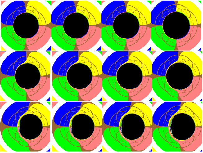
Figure 1: Shadows of a Kerr black hole casted by the extraordinary rays with different coupling parameter $\alpha$ and spin parameter $a$ for the observer in the equatorial plane ($\theta_{obs}=\pi/2$). The top, middle and bottom rows respectively denote the cases with $a=0$, $0.5$, and $0.998$. In each row, the figures from left to right correspond to $\alpha=0$, $0.1$, $0.2$ and $0.3$, respectively.Here we set the mass parameter $M=1$ and $r_{obs}=50M$.

Figs.1 and 2 present Kerr black hole shadows under the axion-photon coupling for different spin parameters. To demonstrate the deformation near the black hole arising from strong gravitational lensing, we divide the total celestial sphere into four quadrants painted in different colors (green, blue, red, and yellow) sw ; swo ; astro ; chaotic ; binary ; sha18 ; my ; swo7 ; swo8 ; swo9 ; swo10 and draw the grids of longitude and latitude lines marked with adjacent brown lines separated by $10^{\circ}$. Actually, the points with different colors in each panel are images of the source points lied in the four different quadrants, which entirely demonstrate the deformation near the black hole originating from strong gravitational lensing. The black parts denote black hole shadows and the white rings provide a direct demonstration of Einstein rings.

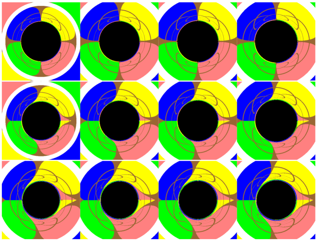
Figure 2: Shadows of a Kerr black hole casted by the extraordinary rays with different coupling parameter $\alpha$ and spin parameter $a$ for the observer along the rotation axis of black hole ($\theta_{obs}=0^{\circ}$). The top, middle and bottom rows respectively denote the cases with $a=0$, $0.5$, and $0.998$. In each row, the figures from left to right correspond to $\alpha=0$, $0.1$, $0.2$ and $0.3$, respectively. Here we set the mass parameter $M=1$ and $r_{obs}=50M$.

Fig.1 presents the Kerr black hole shadows observed in the equatorial plane. It shows that the coupling parameter $\alpha$ results in a larger size of shadows for arbitrary spin parameter $a$. Moreover, for the rapid rotating black hole, its shadow has a usual “D” type shape as the coupling parameter $\alpha$ is smaller. With the increasing of $\alpha$, we find that there exist a “pedicel”-like structure gradually appeared in the left of the shadow, which is similar to those in shadows of a disformal Kerr black hole in quadratic degenerate higher-order scalar-tensor (DHOST) theory fen10 . As the observer stands along the direction of the rotation axis of black hole ($\theta_{obs}=0^{\circ}$), the black hole shadows in Fig.2 have a shape of a circular disk. With the increase of $\alpha$, the size of shadows slightly increases. This is also consistent with the effects of $\alpha$ on the shadow observed in the equatorial plane.

		Sgr A*				M87 *
$\theta_{d}$		$\alpha$				$\alpha$
$(\mu as)$		$0$	$0.1$	$0.2$	$0.3$	$0$	$0.1$	$0.2$	$0.3$
$a$	0.0	51.190	51.530	52.530	54.161	39.611	39.874	40.648	41.910
	0.5	50.900	51.230	52.210	53.811	39.085	39.340	40.114	41.368
	0.998	49.929	50.249	51.180	$52.700$	37.111	37.358	$38.109$	39.332

Table 1: Numerical estimation of the angular diameter of the black shadows of the supermassive black holes Sgr A* and M87* in the theoretical model with the axion-photon coupling.

In Table I, we compare the shadow size of the Kerr black hole with the shadow size of the Sgr A* and M87* black holes with different coupling values of $\alpha$. Here, we use the mass $M=4.0\times 10^{6}M_{\odot}$, the observer distance $D_{O}=8.0kpc$, and the inclination angle $50^{\circ}$ for the black hole Sgr A* and the mass $M=6.5\times 10^{9}M_{\odot}$, the observer distance $D_{O}=16.8Mpc$, and the inclination angle $17^{\circ}$ for the black hole M87*. The angular diameter $\theta_{d}$ does not depend on the coupling parameter $\alpha$ in the nonrotating black hole case but increases with $\alpha$ in the rotating black hole. The effect of $\alpha$ on the angular diameter $\theta_{d}$ increases with the black hole spin parameter. These properties of shadow are consistent with those in the previous discussion. The latest observation indicates that the angular diameters of the black holes M87* and Sgr A* are $\theta_{d}=42\pm 3\mu as$ fbhs1 and $\theta_{d}=48.7\pm 7\mu as$ fbhs1222 . By combining the data in Table I, we find that there is room for such a theoretical model of the axion-photon coupling.

IV summary

We have investigated the motion for photons in the Kerr black hole spacetime under the axion-photon coupling. Although the axion-photon coupling yields birefringence, the birefringence phenomena can be negligible in the small $\alpha$ approximation because the leading-order contributions to the equations of motion come from the corrected terms contained the factor $\alpha^{2}$. We also probe the effects of the coupling on the black hole shadow. It shows that the coupling parameter $\alpha$ makes the size of shadows slightly increase for arbitrary spin parameter $a$. Moreover, for the rapid rotating black hole, its shadow observed in the equatorial plane has a usual “D” type shape as the coupling parameter $\alpha$ is smaller. With the increasing of $\alpha$, we find that there exist a “pedicel”-like structure gradually appeared in the left of the shadow. Finally, we compare the shadow size of the Kerr black hole with the shadow size of the Sgr A* and M87* black holes with different coupling values of $\alpha$ and find that there is room for such a theoretical model of the axion-photon coupling. These results could help to understand deeply the axion field and their corresponding interactions with electromagnetic field.

V Acknowledgments

This work was supported by the National Natural Science Foundation of China under Grant No.12275078, 11875026, 12035005, and 2020YFC2201400.

References

- (1) The Event Horizon Telescope Collaboration, First M87 Event Horizon Telescope Results. I. The Shadow of the Supermassive Black Hole, Astrophys. J. Lett. 875, L1 (2019).
- (2) The Event Horizon Telescope Collaboration, First M87 Event Horizon Telescope Results. VI. The Shadow and Mass of the Central Black Hole, Astrophys. J. Lett. 875, L6 (2019).
- (3) Event Horizon Telescope Collaboration, K. Akiyama, J. C. Algaba et al.,First M87 Event Horizon Telescope Results. VII. Polarization of the Ring, Astrophys. J. Lett. 910, L12 (2021). arXiv:2105.01169
- (4) Event Horizon Telescope Collaboration, K. Akiyama, J. C. Algaba et al., First M87 Event Horizon Telescope Results. VIII. Magnetic Field Structure near The Event Horizon, Astrophys. J. Lett. 910, L13 (2021). arXiv:2105.01173
- (5) Event Horizon Telescope Collaboration, K. Akiyama, et al., First Sagittarius A* Event Horizon Telescope Results. I. The Shadow of the Supermassive Black Hole in the Center of the Milky Way, Astrophys. J. Lett. 930, L12 (2022).
- (6) Event Horizon Telescope Collaboration, K. Akiyama, et al., First Sagittarius A* Event Horizon Telescope Results. VI. Testing the Black Hole Metric, Astrophys. J. Lett. 930, L17 (2022).
- (7) J. M. Bardeen, in Black Holes (Les Astres Occlus), edited by C. DeWitt and B. DeWitt (Gordon and Breach, New York, 1973), p. 215-239.
- (8) S. Chandrasekhar, The Mathematical Theory of Black Holes (Oxford University Press, New York, 1992).
- (9) Pedro V. P. Cunha, Carlos A. R. Herdeiro, Shadows and strong gravitational lensing: a brief review, Gen. Rel. Grav. 50, 42 (2018).
- (10) V. Perlick, O. Yu, Tsupko, Calculating black hole shadows: Review of analytical studies, Phys. Rep. 947, 1 (2022).
- (11) S. Chen, J. Jing, W. Qian, and B. Wang, Black hole images: A review, Sci. China Phys. Mech. Astron. 66, 260401 (2023).
- (12) M. Wang, S. Chen, J. Jing, Chaotic shadows of black holes: a short review, Commun. Theor. Phys. 74, 097401 (2022).
- (13) X. Liu, S. Chen, and J. Jing, Polarization distribution in the image of a synchrotron emitting ring around a regular black hole, Sci. China Phys. Mech. Astron. 65, 120411(2022).
- (14) S. Wei, Y. Liu, Testing the nature of Gauss-Bonnet gravity by four-dimensional rotating black hole shadow, Eur. Phys. J. Plus 136, 436 (2021), arXiv:2003.07769.
- (15) S. Vagnozzi, et al.,Horizon-scale tests of gravity theories and fundamental physics from the Event Horizon Telescope image of Sagittarius A*, Class. Quant. Grav. 40, 65007 (2023).
- (16) M. Wang, S. Chen, J. Jing, Determination of the spin parameter and the inclination angle by the relativistic images in black hole image, Sci. China Phys. Mech. Astron. 66, 110411(2023), arXiv:2208.10219.
- (17) Z. Hu, Z. Zhong, Pe. Li, M. Guo, B. Chen, QED Effect on Black Hole Shadow, Phys. Rev. D 103, 044057 (2021).
- (18) Z. Zhong, Z. Hu, H. Yan, M. Guo, B. Chen, QED Effects on Kerr Black Hole Shadows immersed in uniform magnetic fields, Phys. Rev. D 104, 104028 (2021).
- (19) X. Zeng, K. He, G. Li, E. Liang, S. Guo, QED and accretion flow models effect on optical appearance of Euler-Heisenberg black holes, Eur. Phys. J. C 82, 764 (2022).
- (20) Y. Huang, S. Chen, J. Jing, Double shadow of a regular phantom black hole as photons couple to the Weyl tensor, Eur. Phys. J. C 76, 594 (2016).
- (21) Z. Zhang, S. Chen, X. Qin, J. Jing, Polarized image of a Schwarzschild black hole with a thin accretion disk as photon couples to Weyl tensor, Eur. Phys. J. C 81, 991 (2021).
- (22) S. Chen, J. Jing, Kerr black hole shadow casted by the extraordinary light rays with Weyl corrections, arXiv:2308.16479.
- (23) C. Li, S. Yan, L. Xue, X. Ren, Y. Cai, D. A. Easson, Y. Yuan, and H. Zhao, Testing the equivalence principle via the shadow of black holes, Phys. Rev. Research 2, 023164 (2020), arXiv:1912.12629 [astro-ph].
- (24) R. D. Peccei and H. R. Quinn, CP Conservation in the Presence of Instantons, Phys. Rev. Lett. 38, 1440 (1977).
- (25) A. Arvanitaki, S. Dimopoulos, S. Dubovsky, N. Kaloper, and J. March-Russell, String Axiverse, Phys. Rev. D, 81, 123530 (2010).
- (26) P. Svrcek, E. Witten,Axions In String Theory, J. High Energy Phys. 06, 051 (2006).
- (27) D. J. E. Marsh, Axion Cosmology, Phys. Rept. 643, 1 (2016).
- (28) L. Maiani, R. Petronzio, and E. Zavattini, Effects of Nearly Massless, Spin Zero Particles on Light Propagation in a Magnetic Field, Phys. Lett. B 175, 359 (1986).
- (29) G. Raffelt and L. Stodolsky, Mixing of the Photon with Low Mass Particles, Phys. Rev. D 37, 1237 (1988).
- (30) P. Sikivie, Experimental Tests of the Invisible Axion, Phys. Rev. Lett. 51, 1415 (1983), [Erratum: Phys. Rev. Lett. 52, 695 (1984)].
- (31) I. G. Irastorza and J. Redondo, New experimental approaches in the search for axion-like particles, Prog. Part. Nucl. Phys. 102, 89 (2018).
- (32) V. Anastassopoulos et al. (CAST), New CAST Limit on the Axion-Photon Interaction, Nature Phys. 13, 584 (2017).
- (33) E. Armengaud et al., Conceptual Design of the International Axion Observatory (IAXO), JINST 9, T05002.
- (34) A. Banerjee, D. Budker, J. Eby, V. V. Flambaum, H. Kim, O. Matsedonskyi, G. Perez, Searching for Earth/Solar Axion Halos, J. High Energy Phys. 09, 004(2020).
- (35) S. J. Asztalos et al., A SQUID-based microwave cavity search for dark-matter axions, Phys. Rev. Lett. 104, 041301 (2010).
- (36) A. Mirizzi and D. Montanino, Stochastic conversions of TeV photons into axion-like particles in extragalactic magnetic fields, JCAP 12, 004 (2009).
- (37) M. Meyer, D. Horns, and M. Raue, First lower limits on the photon-axion-like particle coupling from very high energy gamma-ray observations, Phys. Rev. D 87, 035027 (2013).
- (38) T. Yanagida and M. Yoshimura, Resonant Axion-Photon Conversion in the Early Universe, Phys. Lett. B 202, 301 (1988).
- (39) A. Mirizzi, J. Redondo, and G. Sigl, Constraining resonant photon-axion conversions in the Early Universe, JCAP 08, 001 (2009).
- (40) H. Tashiro, J. Silk, and D. J. E. Marsh, Constraints on primordial magnetic fields from CMB distortions in the axiverse, Phys. Rev. D 88, 125024 (2013).
- (41) Y. Chen, J. Shu, X. Xue, Q. Yuan, Y. Zhao, Probing Axions with Event Horizon Telescope Polarimetric Measurements, Phys. Rev. Lett. 124, 061102 (2020).
- (42) T. Fujita, R. Tazaki and K. Toma, Hunting Axion Dark Matter with Protoplanetary Disk Polarimetry, Phys. Rev. Lett. 122, 191101 (2019).
- (43) A. Gußmann, Polarimetric signatures of the photon ring of a black hole that is pierced by a cosmic axion string, J. High Energy Phys. 08, 160(2021).
- (44) Y. Chen, Y. Liu, R. Lu, Y. Mizuno, J. Shu, X. Xue, Q. Yuan, Y. Zhao, Stringent axion constraints with Event Horizon Telescope polarimetric measurements of M87, Nature Astron. 6(5), 592 (2022).
- (45) K. Nomura, K. Saito, J. Soda, Observing axions through photon ring dimming of black holes, Phys. Rev. D 107, 123505 (2023).
- (46) S. Shakeri, F. Hajkarim, Probing Axions via Light Circular Polarization and Event Horizon Telescope, JCAP 04, 017 (2023).
- (47) R. Yao, X. Bi, J. Wang, P. Yin, Probing Axions via Light Circular Polarization and Event Horizon Telescope, Phys. Rev. D 107, 043031 (2023).
- (48) A. D. Plascencia and A. Urbano, Black hole superradiance and polarization-dependent bending of light, JCAP 04 059 (2018).
- (49) I. T. Drummond, S. J. Hathrell, QED vacuum polarization in a background gravitational field and its effect on the velocity of photons, Phys. Rev. D 22, 343 (1980).
- (50) R. D. Daniels and G. M. Shore, “Faster than light” photons and rotating black holes, Phys. Lett. B 367, 75 (1996).
- (51) R. G. Cai, Propagation of vacuum polarized photons in topological black hole spacetimes, Nucl. Phys. B 524, 639 (1998).
- (52) H. T. Cho, “Faster than light” photons in dilaton black hole spacetimes, Phys. Rev. D 56, 6416 (1997).
- (53) V. A. De Lorenci, R. Klippert, M. Novello, J. M. Salim, Light propagation in nonlinear electrodynamics, Phys. Lett. B 482, 134 (2000).
- (54) N. Breton, Geodesic structure of the Born-Infeld black hole, Class. Quantum Grav. 19, 601 (2002).
- (55) P. V. P. Cunha, C. A. Herdeiro, E. Radu and H. F. Runarsson, Shadows of Kerr black holes with scalar hair , Phys. Rev. Lett. 115, 211102 (2015), [arXiv:1509.00021];
- (56) P. V. P. Cunha, C. A. Herdeiro, E. Radu and H. F. Runarsson, Shadows of Kerr black holes with and without scalar hair, Int. J. Mod. Phys. 25, 1641021 (2016), [arXiv:1605.08293].
- (57) F. H. Vincent, E. Gourgoulhon, C. Herdeiro and E. Radu, Astrophysical imaging of Kerr black holes with scalar hair, Phys. Rev. D 94, 084045 (2016), [arXiv:1606.04246].
- (58) P. V. P. Cunha, J. Grover, C. Herdeiro, E. Radu, H. Runarsson, and A. Wittig, Chaotic lensing around boson stars and Kerr black holes with scalar hair, Phys. Rev. D 94, 104023 (2016).
- (59) J. O. Shipley, and S. R. Dolan, Binary black hole shadows, chaotic scattering and the Cantor set, Class. Quantum Grav. 33, 175001 (2016).
- (60) A. Bohn, W. Throwe, F. Hbert, K. Henriksson, and D. Bunandar, What does a binary black hole merger look like?, Class. Quantum Grav. 32, 065002 (2015), [arXiv: 1410.7775].
- (61) M. Wang, S. Chen, J. Jing, Shadows of Bonnor black dihole by chaotic lensing, Phys. Rev. D 97, 064029 (2018).
- (62) T. Johannsen, Photon Rings around Kerr and Kerr-like Black Holes, Astrophys. J. 777, 170 (2013).
- (63) R. Roy, U. Yajnik, Evolution of black hole shadow in the presence of ultralight bosons, Phys. Lett. B 803, 135284 (2020).
- (64) Z. Younsi, A. Zhidenko, L. Rezzolla, R. Konoplya and Y. Mizuno, New method for shadow calculations: Application to parametrized axisymmetric black holes, Phys. Rev. D 94, 084025 (2016).
- (65) M. Wang, S. Chen and J. Jing, Chaotic shadow of a non-Kerr rotating compact object with quadrupole mass, Phys. Rev. D 98 104040 (2018).
- (66) F. Long, S. Chen, M. Wang, J. Jing, Shadow of a disformal Kerr black hole in quadratic degenerate higher-order scalar-tensor theories, Eur. Phys. J. C 80, 1180 (2020).