The role of magnetic waves in tangent cylinder convection

Abstract

The secular variation of the geomagnetic field suggests that there are anticyclonic polar vortices in the Earth’s core. Under the influence of a magnetic field, the polar azimuthal flow is thought to be produced by one or more coherent upwellings within the tangent cylinder, offset from the rotation axis. In this study, convection within the tangent cylinder in rapidly rotating dynamos is investigated through the analysis of forced magnetic waves. The first part of the study investigates the evolution of an isolated buoyancy disturbance in an unstably stratified rotating fluid subjected to an axial magnetic field. It is shown that the axial flow intensity of the slow Magnetic-Archimedean-Coriolis (MAC) waves becomes comparable to that of the fast MAC waves when $|\omega_{M}/\omega_{C}|\sim 0.1$, where $\omega_{M}$ and $\omega_{C}$ are the Alfvén wave and inertial wave frequencies respectively. In spherical shell dynamo simulations, the isolated upwellings within the tangent cylinder are shown to originate from the localized excitation of slow MAC waves in the dipole-dominated regime. Axial flow measurements in turn reveal the approximate parity between the slow and fast wave intensities in this regime, which corresponds to the existence of strong polar vortices in the Earth’s core. To obtain the observed peak azimuthal motions of $0.6$–$0.9^{\circ}$yr^-1, the Rayleigh number in the low-inertia geodynamo must be $\sim 10^{3}$ times the Rayleigh number for the onset of nonmagnetic convection. However, if the forcing is so strong as to cause polarity reversals, the field within the tangent cylinder decays away, and the convection takes the form of an ensemble of plumes supported entirely by the fast waves of frequency $\omega\sim\omega_{C}$. The resulting weak polar circulation is comparable to that obtained in nonmagnetic convection.

1 Introduction

Convection in the Earth’s outer core is separated into two regions by rapid rotation, inside and outside the tangent cylinder (TC). The TC is an imaginary cylinder tangent to the inner core boundary (ICB) and parallel to the Earth’s rotation axis $z$. It cuts the core–mantle boundary (CMB) at approximately latitude 70^∘. Inside the TC, the heat and compositional flux have a substantial component in the $z$ direction, so fluid motions are strongly $z$-dependent. Because ageostrophic motions are needed to transport heat and light elements from the ICB to the CMB inside the TC (Jones, 2015), the forcing needed to initiate convection inside the TC is much higher than that outside it.

The convection inside the TC is thought to be instrumental in the generation of anticyclonic polar vortices in the core, suggested by observations of secular variation (Olson and Aurnou, 1999; Hulot et al., 2002). Nonmagnetic laboratory experiments that simulate the TC region (Aurnou et al., 2003; Aujogue et al., 2018) suggest that an ensemble of convection plumes extending from the ICB to latitudes greater than 70^∘ would make the poles warmer than the equator, resulting in an anticyclonic circulation near the poles. Numerical simulations of the geodynamo (Sreenivasan and Jones, 2005, 2006), on the other hand, show that the structure of convection inside the TC is often dominated by an isolated off-axis plume that generates a strong anticyclonic flow near the poles. The fluid inside the rising plume is systematically warmer than the cold descending fluid outside the plume. The Coriolis force then acts to turn the radially outward flow at the top of the plume into an anticyclonic vortex. The intensity of polar vortices in the dynamo is much greater than that in nonmagnetic convection (Sreenivasan and Jones, 2005), which indicates that the vortices are magnetically enhanced.

The tangent cylinder may be approximated by a rotating plane layer in which convection takes place under a predominantly $z$ magnetic field. The onset of magnetoconvection in a rotating plane layer occurs either as thin viscously controlled columns or large-scale magnetic rolls (Chandrasekhar, 1961). For a field that is either uniform or of a length scale comparable to the depth of the fluid layer, large-scale magnetically controlled convection sets in at relatively small Elsasser numbers $\varLambda=O(E^{1/3})$ (Zhang, 1995; Jones et al., 2003), where $\varLambda$ is the square of the scaled mean magnetic field and $E$ is the Ekman number that measures the ratio of viscous to Coriolis forces. However, for the spatially inhomogeneous magnetic field in a dynamo (e.g. Schaeffer et al., 2017), the viscous–magnetic mode transition may not take place even at $\varLambda=O(1)$ (Gopinath and Sreenivasan, 2015). In a dipole-dominated dynamo, the field generated outside the TC diffuses into the TC and gets concentrated on scales comparable to that of the thin plumes that form at the onset of convection. The lateral inhomogeneity of the magnetic flux gives rise to an instability where convection is entirely confined to the peak-field region (Sreenivasan and Gopinath, 2017). This pattern of convection inside the TC may be understood in terms of fast and slow Magnetic-Archimedean-Coriolis (MAC) waves that form in a rapidly rotating Bénard layer permeated by a magnetic field. The fast waves are linear inertial waves weakly modified by the magnetic field and buoyancy while the slow waves are magnetostrophic waves produced by the balance between the magnetic, Coriolis and buoyancy forces (Braginsky, 1967; Acheson and Hide, 1973). The magnetic flux concentrations within the TC may locally produce unstable stratification, thereby supporting convection through slow MAC waves. In regions where the magnetic flux is weak, the fast MAC waves generated at the base of the TC are rendered ineffectual in transporting heat and light elements through the neutrally buoyant layer. In this way, a laterally varying magnetic field can give rise to an isolated off-axis plume within the TC. If the buoyant forcing in the dynamo is so strong as to cause the collapse of the axial dipole field outside the TC, the field intensity within the TC would be considerably reduced. Consequently, the convection may take the form of an ensemble of plumes supported by fast waves, akin to that found in the nonmagnetic state.

The present study builds on earlier work (Sreenivasan and Maurya, 2021) that investigated the evolution of an isolated buoyancy disturbance in a rapidly rotating fluid under a uniform axial magnetic field. Of particular interest is the regime where the ratio of Alfvén wave to inertial wave frequencies $|\omega_{M}/\omega_{C}|\sim 0.1$, thought to be relevant to dipole-dominated dynamos. Subsequently, Majumder et al. (2023) demonstrated that the collapse of the axial dipole in rapidly rotating dynamos occurs when the slow MAC waves disappear under strong forcing. Here, TC convection in dipole-dominated and polarity-reversing dynamos is understood through the analysis of forced magnetohydrodynamic waves in the inertia-free limit, where the ratio of nonlinear inertia to Coriolis forces is small not only on the core depth but also on the length scale of convection. It is shown that slow MAC waves are essential for the generation of strong polar vortices in dipole-dominated dynamos.

In Section 2, a simplified linear model of the TC is considered wherein a buoyancy disturbance evolves in an unstably stratified rotating fluid subject to an axial magnetic field. It is shown that the intensity of the slow MAC waves would be at least as high as that of the fast waves for $Le\sim 0.1$, where $Le$ measures the ratio of Alfvén wave to inertial wave frequencies. Section 3 investigates TC convection in spherical dynamo simulations at progressively increasing forcing spanning the dipole-dominated regime up to the onset of polarity reversals. The measurement of wave motions within the TC enables a comparison of the dynamics with that predicted by the simplified linear model. The main results of this paper are summarized in Section 4.

2 A tangent cylinder model: Evolution of an isolated buoyancy disturbance

Since the dominant magnetic field within the tangent cylinder is known to be axial, we consider the evolution of a density perturbation $\rho^{\prime}$ under gravity $\bm{g}=-g\ \hat{\bm{e}}_{z}$, a uniform axial magnetic field $\bm{B}=B\hat{\bm{e}}_{z}$ and background rotation $\bm{\varOmega}=\varOmega\hat{\bm{e}}_{z}$ (figure 1). In cylindrical polar coordinates $(s,\phi,z)$, this perturbation is symmetric about its own axis, or in other words, independent of $\phi$. Since $\rho^{\prime}$ is related to a temperature perturbation $\theta$ by $\rho^{\prime}=-\rho\alpha\theta$, where $\rho$ is the ambient density and $\alpha$ is the coefficient of thermal expansion, an initial temperature perturbation is chosen in the form

$$\theta_{0}=A\exp\left[-2(s^{2}+z^{2})/\delta^{2}\right],$$ (1)

where $A$ is a constant and $\delta$ is the length scale of the perturbation.

2.1 Governing equations and solutions

In the Boussinesq approximation, the following linearized MHD equations describe the evolution of $\bm{u}$, $\bm{b}$ and $\theta$:

$$\frac{\partial{\bm{u}}}{\partial{t}}=-\frac{1}{\rho}\nabla{p^{*}}-2\bm{\varOmega}\times\bm{u}+\frac{1}{\mu\rho}\left(\bm{B}\cdot\nabla\right)\bm{b}-\bm{g}\alpha\theta+\nu\nabla^{2}\bm{u},$$ (2)

$$\frac{\partial{\bm{b}}}{\partial{t}}=\left(\bm{B}\cdot\nabla\right){\bm{u}}+\eta\nabla^{2}\bm{b},$$ (3)

$$\frac{\partial{\theta}}{\partial{t}}=-\beta\bm{\hat{e}}_{z}\cdot\bm{u}+\kappa\nabla^{2}\theta,$$ (4)

$$\nabla\cdot\bm{u}=\nabla\cdot\bm{b}=0,$$ (5)

where $\nu$ is the kinematic viscosity, $\kappa$ is the thermal diffusivity, $\eta$ is the magnetic diffusivity, $\mu$ is the magnetic permeability, $p^{*}=p-(\rho/2)|\bm{\varOmega}\times\bm{x}|^{2}+(\bm{B}\cdot\bm{b})/\mu$ and $\beta=\partial T_{0}/\partial z<0$ is the mean axial temperature gradient in the unstably stratified fluid.

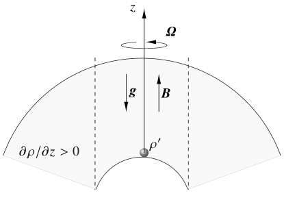
Figure 1: A density perturbation $\rho^{\prime}$ evolves in an unstably stratified fluid layer under a uniform axial magnetic field $\bm{B}$ and background rotation $\bm{\varOmega}$.

In a quiescent fluid, the initial velocity $\bm{u}_{0}$ is zero, and since the magnetic field perturbation takes finite time to develop by induction, the initial induced field $\bm{b}_{0}$ is also zero. The initial temperature perturbation (1) produces a poloidal flow which interacts with $\bm{\varOmega}$ to generate a toroidal flow, so that the instantaneous state of the flow is defined by (Sreenivasan and Maurya, 2021)

$$\bm{u}=u_{\phi}\hat{\bm{e}}_{\phi}+\nabla\times[(\psi/s)\hat{\bm{e}}_{\phi}],$$ (6)

$$\nabla_{*}^{2}\psi=\frac{\partial^{2}\psi}{\partial z^{2}}+s\frac{\partial}{\partial s}\left(\frac{1}{s}\frac{\partial\psi}{\partial s}\right)=-s\zeta_{\phi},$$ (7)

where $\psi$ is the Stokes streamfunction of the velocity and $\bm{\zeta}$ is the vorticity. Likewise, the instantaneous state of the induced magnetic field is defined by,

$$\bm{b}=b_{\phi}\hat{\bm{e}}_{\phi}+\nabla\times[(\xi/s)\hat{\bm{e}}_{\phi}],$$ (8)

$$\nabla_{*}^{2}\xi=-s\mu j_{\phi},$$ (9)

where $\xi$ is the Stokes streamfunction of the induced magnetic field and $\bm{j}$ is the electric current density.

Algebraic simplifications of the governing equations give an equation for the evolution of $\psi$ in the form (Sreenivasan and Maurya, 2021)

$$\bigg{[} \left(\frac{\partial{}}{\partial{t}}-\nu\nabla_{*}^{2}\right)\left(\frac{\partial{}}{\partial{t}}-\eta\nabla_{*}^{2}\right)-V_{M}^{2}\frac{\partial^{2}}{\partial{z^{2}}}\bigg{]}^{2}\left(\frac{\partial{}}{\partial{t}}-\kappa\nabla_{*}^{2}\right)\left(\nabla_{*}^{2}\psi\right)$$ (10)

$$= -4\varOmega^{2}\,\left(\frac{\partial{}}{\partial{t}}-\kappa\nabla_{*}^{2}\right)\left(\frac{\partial{}}{\partial{t}}-\eta\nabla_{*}^{2}\right)^{2}\frac{\partial^{2}{\psi}}{\partial{z^{2}}}$$

$$-g\alpha\beta s\,\left(\frac{\partial{}}{\partial{t}}-\eta\nabla_{*}^{2}\right)\left[\left(\frac{\partial{}}{\partial{t}}-\nu\nabla_{*}^{2}\right)\left(\frac{\partial{}}{\partial{t}}-\eta\nabla_{*}^{2}\right)-V_{M}^{2}\frac{\partial^{2}}{\partial{z^{2}}}\right]\frac{\partial{}}{\partial{s}}\left(\frac{1}{s}\frac{\partial{\psi}}{\partial{s}}\right),$$

where $V_{M}=B/\sqrt{\mu\rho}$ is the Alfvén wave velocity.

By applying the Hankel–Fourier transform

$$H_{1}\{\psi(s,z)/s\}=\hat{\psi}(k_{s},k_{z})=\frac{1}{2\pi^{2}}\int_{0}^{\infty}\int_{0}^{\infty}\psi(s,z)J_{1}(k_{s}s)\mbox{e}^{-ik_{z}z}\,\mbox{d}s\,\mbox{d}z$$ (11)

to (10), where $J_{1}$ is the first-order Bessel function of the first kind, we obtain,

$$\bigg{[} \left(\frac{\partial{}}{\partial{t}}+\nu k^{2}\right)\left(\frac{\partial{}}{\partial{t}}+\eta k^{2}\right)+V_{M}^{2}k_{z}^{2}\bigg{]}^{2}\left(\frac{\partial{}}{\partial{t}}+\kappa k^{2}\right)\hat{\psi}$$ (12)

$$= -\frac{4\varOmega^{2}k_{z}^{2}}{k^{2}}\left(\frac{\partial{}}{\partial{t}}+\eta k^{2}\right)^{2}\left(\frac{\partial{}}{\partial{t}}+\kappa k^{2}\right)\hat{\psi}$$

$$-\frac{g\alpha\beta k_{s}^{2}}{k^{2}}\left(\frac{\partial{}}{\partial{t}}+\eta k^{2}\right)\left[\left(\frac{\partial{}}{\partial{t}}+\nu k^{2}\right)\left(\frac{\partial{}}{\partial{t}}+\eta k^{2}\right)+V_{M}^{2}k_{z}^{2}\right]\hat{\psi}.$$

Considering plane wave solutions of the form $\hat{\psi}\sim\mbox{e}^{i\lambda t}$, we obtain the relation

$$\lambda^{5} -2i\omega_{\eta}\lambda^{4}-\left(\omega_{A}^{2}+\omega_{\eta}^{2}+2\omega_{M}^{2}+\omega_{C}^{2}\right)\lambda^{3}+2i\omega_{\eta}\left(\omega_{A}^{2}+\omega_{M}^{2}+\omega_{C}^{2}\right)\lambda^{2}$$ (13)

$$+\left(\omega_{A}^{2}\omega_{\eta}^{2}+\omega_{A}^{2}\omega_{M}^{2}+\omega_{M}^{4}+\omega_{\eta}^{2}\omega_{C}^{2}\right)\lambda-i\omega_{A}^{2}\omega_{\eta}\omega_{M}^{2}=0.$$

for a system where both viscous and thermal diffusion are much smaller than magnetic diffusion ($\nu,\kappa\to 0$).

The fundamental frequencies in (13) are given by,

$$\omega_{C}^{2}=\frac{4\varOmega^{2}k_{z}^{2}}{k^{2}},\quad\omega_{M}^{2}=V_{M}^{2}k_{z}^{2},\quad\omega_{A}^{2}=g\alpha\beta\frac{k_{s}^{2}}{k^{2}},\quad\omega_{\eta}^{2}=\eta^{2}k^{4},$$ (14a-d)

representing linear inertial waves, Alfvén waves, internal gravity waves and magnetic diffusion respectively. In unstable density stratification, $\omega_{A}^{2}<0$. Here, $k^{2}=k_{s}^{2}+k_{z}^{2}$.

For the frequency inequality $|\omega_{C}|\gg|\omega_{M}|\gg|\omega_{A}|\gg|\omega_{\eta}|$, the roots of equation (13) are approximated by (Sreenivasan and Maurya, 2021)

$$\lambda_{1,2} \approx \pm\left(\omega_{C}+\frac{\omega_{M}^{2}}{\omega_{C}}\right)+i\,\frac{\omega_{M}^{2}\omega_{\eta}}{\omega_{C}^{2}},$$ (15)

$$\lambda_{3,4} \approx \pm\left(\frac{\omega_{M}^{2}}{\omega_{C}}+\frac{\omega_{A}^{2}}{2\omega_{C}}\right)+i\,\omega_{\eta}\,\left(1-\frac{\omega_{A}^{2}}{2\omega_{M}^{2}}\right),$$ (16)

$$\lambda_{5} \approx i\,\frac{\omega_{A}^{2}\omega_{\eta}}{\omega_{M}^{2}},$$ (17)

representing damped fast MAC waves ($\lambda_{1,2}$), damped slow MAC waves ($\lambda_{3,4}$), and the overall growth of the perturbation ($\lambda_{5}$).

The general solutions for $\hat{\psi}$, $\hat{u_{\phi}}$, $\hat{\xi}$, $\hat{b_{\phi}}$ are then given by

$$=\sum_{m=1}^{5}[D_{m},G_{m},P_{m},Q_{m}]\mbox{e}^{i\lambda_{m}t},$$ (18)

where the coefficients $D_{m}$, $G_{m}$, $P_{m}$ and $Q_{m}$ are evaluated from the initial conditions for $\hat{\psi}$, $\hat{u_{\phi}}$, $\hat{\xi}$, $\hat{b_{\phi}}$ and their time derivatives. The poloidal velocity is obtained from its streamfunction using the relations

$$\hat{u}_{z}=k_{s}\hat{\psi},\quad\hat{u}_{s}=-ik_{z}\hat{\psi}.$$ (19a-b)

2.2 MAC waves in unstable stratification

The analysis of the solutions is limited to times much shorter than the time scale for the exponential increase of the perturbations. When the buoyancy force is small compared with the Lorentz force ($|\omega_{A}/\omega_{M}|\ll 1$), the parameter regime is determined by the Lehnert number $Le$ and the magnetic Ekman number $E_{\eta}$,

$$Le=\frac{V_{M}}{2\varOmega\delta},\quad E_{\eta}=\frac{\eta}{2\varOmega\delta^{2}},$$ (20a-b)

based on the length scale of the initial perturbation (1).

Figure 2 shows the evolution in time of the poloidal velocity streamfunction, obtained from the inverse Hankel–Fourier transform

$$\psi(s,z)=4\pi s\int_{0}^{\infty}\int_{0}^{\infty}\hat{\psi}(k_{s},k_{z})J_{1}(k_{s}s)\mbox{e}^{ik_{z}z}k_{s}dk_{s}dk_{z},$$ (21)

computed by setting the upper limits of the integrals (the truncation values of $k_{s}$ and $k_{z}$) to $3/\delta$. The formation of a columnar structure from the initial perturbation through wave motions is evident.

(a)                                 (b)                                 (c)

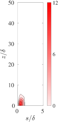
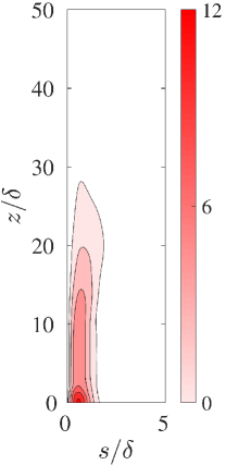
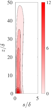
Figure 2: Evolution of the poloidal velocity streamfunction $\psi$ with time (measured in units of the magnetic diffusion time $t_{\eta}$) for $Le=0.09$ and $E_{\eta}=2\times 10^{-5}$. The snapshots are at (a) $t/t_{\eta}=1\times 10^{-3}$, (b) $t/t_{\eta}=5\times 10^{-3}$ and (c) $t/t_{\eta}=1\times 10^{-2}$. The ratio $|\omega_{A}/\omega_{M}|=0.05$ at times after the formation of the waves.

In figure 3 (a), the fundamental frequencies are based on the mean wavenumbers obtained from ratios of $L^{2}$ norms,

$$\bar{k}_{s}=\frac{||k_{s}\hat{\psi}k||}{||\hat{\psi}k||},\quad\bar{k}_{z}=\frac{||k_{z}\hat{\psi}k||}{||\hat{\psi}k||},\quad\bar{k}=\frac{||\hat{\psi}k^{2}||}{||\hat{\psi}k||}.$$ (22a-c)

For $Le>0.005$, the inequality $|\omega_{C}|>|\omega_{M}|>|\omega_{A}|$ exists, indicating the MAC wave regime. To obtain the relative intensities of the fast and slow MAC waves, the fast and slow MAC wave parts of the general solution are separated, as in earlier studies (Sreenivasan and Narasimhan, 2017; Sreenivasan and Maurya, 2021).

The kinetic energy is calculated using the Parseval’s theorem,

$$E_{k}=16\pi^{4}\int_{0}^{\infty}\int_{0}^{\infty}\left(\hat{u}_{s}^{2}+\hat{u}_{z}^{2}+\hat{u}_{\phi}^{2}\right)k_{s}\mbox{d}k_{s}\mbox{d}k_{z},$$ (23)

separately for the fast and slow MAC waves, with the upper limits of the integrals set to $10/\delta$ in the computations.

Figure 3 (b) shows the variation of the total kinetic energy $E_{k}$ of the two waves with $|\omega_{M}/\omega_{C}|$. The range of $|\omega_{M}/\omega_{C}|$ in figure 3 (b) corresponds to the range of $Le$ in figure 3 (a). Both $Le$ and $|\omega_{M}/\omega_{C}|$ are of the same order of magnitude when the magnetic field and rotation axes are parallel (Sreenivasan and Maurya, 2021). (Since the initial wavenumber $k_{0}=\sqrt{6}/\delta$, $|\omega_{M}/\omega_{C}|=\sqrt{6}\,Le$.) The slow MAC waves appear when $\omega_{M}$ exceeds $\omega_{A}$, and their energy becomes comparable to that of the fast waves for $Le\sim 0.1$. Figure 3 (c) shows that the peak value of the slow wave $z$ velocity is approximately equal to that of fast waves when $|\omega_{M}/\omega_{C}|\approx 0.2$, where $u_{z}=s^{-1}\,\partial\psi/\partial s$. Figure 3 (d) shows the peak value of $u_{z}$ for both fast and slow waves against $|\omega_{A}/\omega_{M}|$ at $Le=0.09$ ($|\omega_{M}/\omega_{C}|=0.22$). The slow wave velocity decreases appreciably and tends to zero as $|\omega_{A}/\omega_{M}|\approx 1$. The fast wave velocity, on the other hand, does not change much with increasing buoyancy. Figures 3 (a)–(d) indicate that the intensity of slow MAC wave motions would be comparable to that of the fast waves in the regime thought to be relevant to dipole-dominated dynamos, $|\omega_{M}/\omega_{C}|\sim 0.1$ and $|\omega_{A}/\omega_{M}|<1$. In the regime $|\omega_{A}/\omega_{M}|\sim 1$, where dipole collapse is found to happen (Majumder et al., 2023), the slow MAC wave velocity goes to zero. The effect of increasing buoyancy on the fast and slow MAC waves are shown graphically in figure 4. Here, the magnitudes of the fast and slow waves are comparable at $|\omega_{A}/\omega_{M}|=0.1$, whereas the slow waves are severely attenuated for $|\omega_{A}|\sim|\omega_{M}|$. The fast waves are practically unaffected by the increased forcing.

Figure 5 shows the variation of the $\phi$ component of kinetic energy, normalized by its nonmagnetic value, with progressively increasing forcing for a given $\omega_{M}/\omega_{C}$. As $|\omega_{A}/\omega_{M}|$ tends to unity, the energy tends to the nonmagnetic value, consistent with the suppression of the slow waves. This result has implications for the intensity of polar vortices in strongly forced dynamos where $|\omega_{A}/\omega_{M}|\sim 1$ within the tangent cylinder.

In Section 3, we examine whether slow MAC waves are influential in the generation of strong polar vortices in dipole-dominated spherical dynamos. We also study the regime of dipole collapse, wherein we expect TC convection to be supported by only the fast waves, resulting in much weaker polar circulation.

(a)                                                         (b)

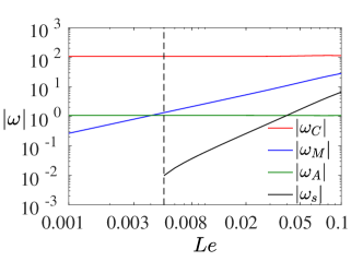
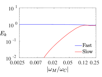
(c)                                                         (d)

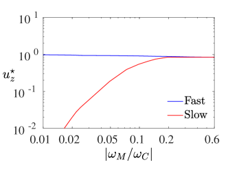
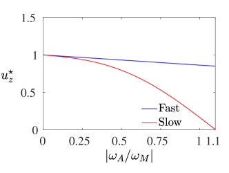
Figure 3: (a) Variation of absolute values of the frequencies with Lehnert number $Le$. (b) Variation of the kinetic energy of fast and slow MAC waves (normalized by the nonmagnetic kinetic energy) with $|\omega_{M}/\omega_{C}|$. The range of $|\omega_{M}/\omega_{C}|$ in (b) corresponds to the range of $Le$ in (a). Here, $|\omega_{A}/\omega_{M}|=0.1$. (c) Variation of the peak values of the fast and slow wave parts of the $z$ velocity (normalized by its nonmagnetic value) with $|\omega_{M}/\omega_{C}|$. (d) Variation of the peak $z$ velocity of fast and slow MAC waves with $|\omega_{A}/\omega_{M}|$ for $Le=0.09$. All calculations are performed for $E_{\eta}=2\times 10^{-5}$ and $t/t_{\eta}=5\times 10^{-3}$.

(a)                                 (b)                                 (c)

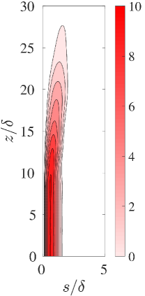
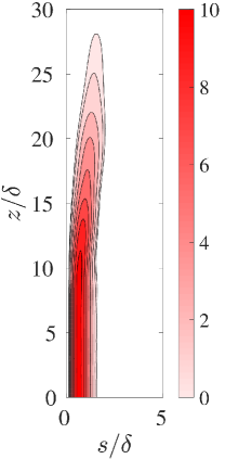
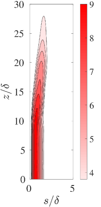
(d)                                 (e)                                 (f)

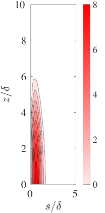
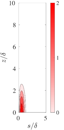
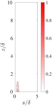
Figure 4: Streamfunction $\psi$ of the fast wave part of the solution ((a)–(c)), and that for the slow wave part ((d)–(f)) for $|\omega_{A}/\omega_{M}|=0.1,0.6,0.95$ (shown left to right). The plots are generated at time $t/t_{\eta}=5\times 10^{-3}$ for the parameters $Le=0.09$ and $E_{\eta}=2\times 10^{-5}$.

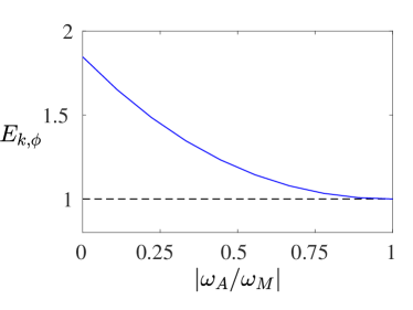
Figure 5: Variation with $|\omega_{A}/\omega_{M}|$ of the $\phi$ component of the kinetic energy, $E_{k,\phi}$ normalized by its nonmagnetic value. The calculations are performed for $E_{\eta}=2\times 10^{-5}$, $t/t_{\eta}=5\times 10^{-3}$ and $|\omega_{M}/\omega_{C}|=0.225$.

3 Nonlinear dynamo simulations

We consider an electrically conducting fluid located between two concentric, co-rotating spherical surfaces with a radius ratio of 0.35. These surfaces correspond to the inner core boundary (ICB) and the core-mantle boundary (CMB). Our model is based on the codensity formulation, where thermal and compositional buoyancy are combined (Braginsky and Roberts, 1995). The other two body forces are the Lorentz force, which arises from the interaction between the induced electric current and the magnetic field, and the Coriolis force, which originates from the background rotation.

In the dynamo models, lengths are scaled by the thickness of the spherical shell $L$ and the time is scaled by magnetic diffusion time $L^{2}/\eta$, where $\eta$ is magnetic diffusivity. The velocity field $\bm{u}$ is scaled by $\eta/L$, while the magnetic field $\bm{B}$ is scaled by $(2\varOmega\rho\mu\eta)^{1/2}$, where $\varOmega$ represents the rotation rate, $\rho$ represents fluid density, and $\mu$ represents magnetic permeability. The temperature is scaled by $\beta L$, where $\beta$ denotes the radial temperature gradient at the outer boundary.

The non-dimensional equations for velocity, magnetic field, and temperature in MHD under the Boussinesq approximation are given by,

$$EPm^{-1}\Bigl{(}\frac{\partial{\bm{u}}}{\partial t}+(\nabla\times{\bm{u}})\times{\bm{u}}\Bigr{)}+{\hat{\bm{z}}}\times{\bm{u}}=-\nabla p^{\star}+Ra\,PmPr^{-1}\,T\,{\bm{r}}\,$$

$$+(\nabla\times{\bm{B}})\times{\bm{B}}+E\nabla^{2}{\bm{u}},$$ (24)

$$\frac{\partial{\bm{B}}}{\partial t}=\nabla\times({\bm{u}}\times{\bm{B}})+\nabla^{2}{\bm{B}},$$ (25)

$$\frac{\partial T}{\partial t}+({\bm{u}}\cdot\nabla)T=PmPr^{-1}\,\nabla^{2}T,$$ (26)

$$\nabla\cdot{\bm{u}}=\nabla\cdot{\bm{B}}=0.$$ (27)

The modified pressure $p^{*}$ in equation (24) is given by $p+\frac{1}{2}E\,Pm^{-1}\,|\bm{u}|^{2}$. The dimensionless parameters in the above equations are the Ekman number $E=\nu/2\varOmega L^{2}$, the Prandtl number, $Pr=\nu/\kappa$; the magnetic Prandtl number, $Pm=\nu/\eta$; and the modified Rayleigh number, given by $g\alpha\beta L^{2}/2\varOmega\kappa$. The parameters $g$, $\nu$, $\kappa$, and $\alpha$ denote the gravitational acceleration, kinematic viscosity, thermal diffusivity, and coefficient of thermal expansion respectively.

The temperature distribution in the basic state is described by a basal heating profile given by $T_{0}(r)=r_{i}r_{o}/r$, where $r_{i}$ and $r_{o}$ are the inner and outer radii of the spherical shell respectively. The velocity and magnetic fields satisfy the no-slip and electrically insulating conditions at their respective boundaries. The inner boundary is isothermal, whereas the outer boundary maintains a constant heat flux. The calculations are performed using a pseudospectral code that applies spherical harmonic expansions to the angular coordinates $(\theta,\phi)$ and finite differences to the radius $r$ (Willis et al., 2007).

For two values of the Ekman number $E$, a series of simulations at progressively increasing Rayleigh number $Ra$ are performed, spanning the dipole-dominated regime up to the start of polarity reversals. For each $E$, the value of $Pm=Pr$ is chosen such that the local Rossby number $Ro_{\ell}$, which gives the ratio of the inertial to Coriolis forces on the characteristic length scale of convection (Christensen and Aubert, 2006) is $<0.1$ (Majumder et al., 2023). Thus, the dynamo simulations lie in the rotationally dominant, or low-inertia, regime. For $Pm=Pr$, the dynamo obtained by solving equations (24)–(27) is compared with its nonmagnetic counterpart, obtained by solving equations (31)–(33), A.

3.1 TC convection and polar vortices

(a)                                         (b)                                            (c)
     
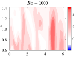
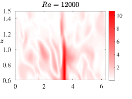
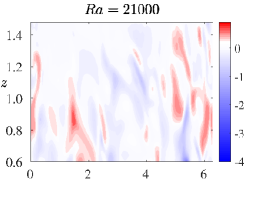
(d)                                         (e)                                            (f)

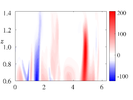
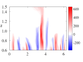
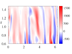
(g)                                         (h)                                            (i)

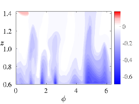
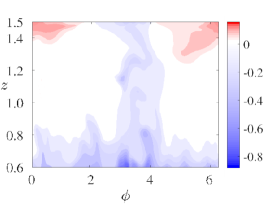
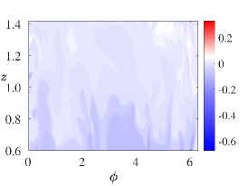
Figure 6: Cylindrical section ($z-\phi$) plots within the tangent cylinder of $B_{z}$ (a-c), $u_{z}$ (d-f) and $\partial T/\partial z$ (g-i) for $E=6\times 10^{-5},Pr=Pm=5$. The figures are shown from the saturated state of the dynamo simulation. The Rayleigh number $Ra$ in the simulation is given above the panels.

(a)                                         (b)

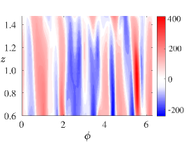
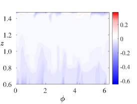
Figure 7: Cylindrical section ($z-\phi$) plots within the tangent cylinder of $u_{z}$ (a) and $\partial T/\partial z$ (b) for the nonmagnetic convection simulation at $E=6\times 10^{-5}$, $Ra=12000$ and $Pr=5$.

In Figure 6, a cylindrical ($z$-$\phi$) section at selected cylindrical radii $s$ of the axial field $B_{z}$, axial flow $u_{z}$ and axial temperature gradient $\partial T/\partial z$ are shown. The dynamo parameters are $E=6\times 10^{-5}$ and $Pm=Pr=5$. At $Ra=1000$, the magnetic flux that diffuses into the TC from outside appears to concentrate on length scales comparable to that at convective onset. Because of the convergent flow at the base of an upwelling (Sreenivasan and Jones, 2006), $B_{z}$ typically concentrates near the base of the TC. A plume appears at the same location as the flux concentration (figures 6 (a) and (d)), and the same behaviour is reproduced at much stronger forcing (figures 6 (b) and (e)). Outside the plume, where the magnetic flux is weak, convection is absent except at the base of TC. This suppression of convection, also noted in linear magnetoconvection with a laterally varying field (Sreenivasan and Gopinath, 2017), can be explained by a localized unstable stratification produced by the magnetic field through a magnetic-Coriolis balance (figures 6 (g) and (h)). Elsewhere, the fluid layer is neutrally buoyant. There are stably stratified regions with $\partial T/\partial z>0$ at the top of TC, where warm fluid carried upward by the plume builds up. When buoyant forcing is increased to the point of polarity reversals outside the TC, there is no coherent magnetic flux concentration within the TC (figure 6 (c)); then convection takes the form of an ensemble of plumes (figure 6 (f)), similar to that found in nonmagnetic simulations (see figure 7 (a)). In both nonmagnetic and reversing simulations, the entire fluid layer is unstably stratified (figures 7 (b) and 6 (i)).

The polar vortices produced by the pattern of convection within the TC are shown in the $z$-section plots in figures 8. For a wide range of $Ra$ in the dipole-dominated regime, the correlation between $u_{z}$ and $B_{z}$ exists (figures 8 (a), (b) and (d), (e)); the radially outward motion at the top of the plume is turned into a strong anticyclonic vortex by the Coriolis force (figures 8 (c), (f)). In the strongly driven regime of dipole collapse, the absence of a coherent field results in multi-column convection (figure 8 (g), (h)) and a much weaker anticyclonic circulation near the poles (figure 8 (i)). On time and azimuthal average, the polar vortex intensity increases with $Ra$ (figures 9 (a) and (b)); however, at the point of reversals, the vortex intensity significantly diminishes (figure 9 (c)), resembling that in the nonmagnetic runs (figure 9 (d)).

$B_{z}$                                        $u_{z}$                                        $u_{\phi}$
$Ra=12000$
(a)                                        (b)                                        (c)

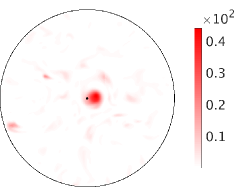
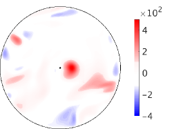
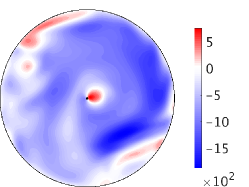
$Ra=18000$
(d)                                        (e)                                        (f)

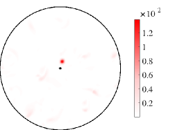
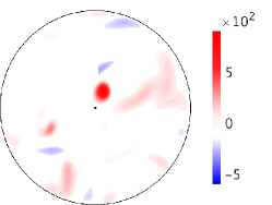
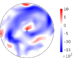
$Ra=21000$
(g)                                        (h)                                        (i)

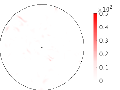
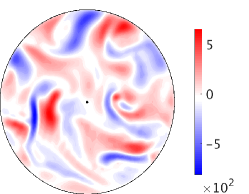
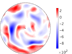
Figure 8: Horizontal $(z)$ section plots within the tangent cylinder of the axial magnetic field $B_{z}$ at $z=0.9$ (left panels), $u_{z}$ at $z=1.4$ (middle panels) and $u_{\phi}$ at $z=1.4$ (right panels) for $Ra=12000$ (a-c), $Ra=18000$ (d-f), $Ra=21000$ (g-i). The other dynamo parameters are $E=6\times 10^{-5},Pm=Pr=5$. The figures are shown from the saturated state of the dynamo simulation.

The maximum dimensionless time and azimuthally averaged value of $u_{\phi}$ is measured within the TC, with its radial distance from the rotation axis. For example, for $Ra=12000$ ($E=6\times 10^{-5},Pm=Pr=5$), this magnitude of $u_{\phi}$ is 508, at radius 0.33. This could be scaled up to its value in the Earth’s core (Sreenivasan and Jones, 2005), giving

$$u_{\phi,\mbox{sc}}=\frac{u_{\phi}\eta}{L}=2.2478\times 10^{-4}\mbox{m}\mbox{s}^{-1}\approx 0.535^{\circ}\mbox{yr}^{-1},$$ (28)

where $\eta$ and $L$ have the values 1 m²s^-1 and $2.26\times 10^{6}$ m respectively. The values of $u_{\phi,\mbox{sc}}$ in the simulations and their respective values in nonmagnetic simulations are given in table 1. Increasing the strength of forcing in the nonmagnetic simulations does not result in stronger polar vortices, which indicates the crucial role of the magnetic field in generating strong polar circulation.

(a)                                        (b)

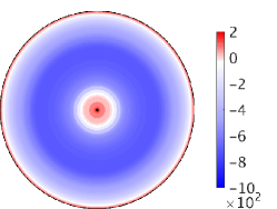
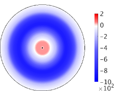
(c)                                        (d)

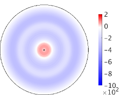
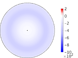
Figure 9: Horizontal $(z)$ section plots at height $z=1.4$ above the equator of the time and azimuthally averaged flow $u_{\phi}$ within the TC at $E=6\times 10^{-5}$, $Pm=Pr=5$. (a) $Ra=$12000, (b) $Ra=$18000, (c) $Ra=$21000, (d) nonmagnetic run at $Ra=$12000. All figures represent the saturated state of the simulations.

3.2 Magnetic waves in the TC

(a)                                                              (b)

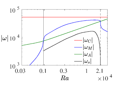
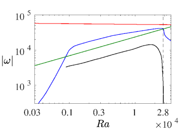
Figure 10: (a, b) Absolute values of the measured frequencies $\omega_{C}$, $\omega_{M}$, $\omega_{A}$, and $\omega_{s}$ inside the tangent cylinder versus the Rayleigh number $Ra$ in the saturated dynamo. The dynamo parameters are (a) $E=6\times 10^{-5}$, $Pm=Pr=5$ and (b) $E=1.2\times 10^{-5}$, $Pm=Pr=1$. The solid vertical lines indicate the onset of the slow MAC waves inside the tangent cylinder while the dashed vertical lines mark the suppression of the slow waves. The onset of the slow waves occurs at $Ra=960$ (a) and $Ra=900$ (b) and their suppression occurs at $Ra=20500$ (a) and $Ra=27500$ (b).

Isolated density disturbances within the TC evolve as fast and slow MAC waves in the presence of the rapid rotation and magnetic field. Since the frequency of these waves depends on the fundamental frequencies $\omega_{C}$, $\omega_{M}$ and $\omega_{A}$ (Section 2.1), we look at their magnitudes in dimensionless form (Varma and Sreenivasan, 2022),

$$\omega_{C}^{2}=\frac{Pm^{2}}{E^{2}}\frac{k_{z}^{2}}{k^{2}},\quad\omega_{M}^{2}=\frac{Pm}{E}(\bm{B}\cdot\bm{k})^{2},\quad-\omega_{A}^{2}=\frac{Pm^{2}Ra}{PrE}\frac{k_{h}^{2}}{k^{2}},$$ (29a-c)

where the Alfvén frequency is based on the three components of the magnetic field at the peak field location and the frequencies are scaled by $\eta/L^{2}$. Here, $k_{s}$, $k_{\phi}$ and $k_{z}$ are the radial, azimuthal and axial wavenumbers in cylindrical coordinates, $k_{h}$ is the horizontal wavenumber inside the TC given by $k_{h}^{2}=k_{s}^{2}+k_{\phi}^{2}$, and $k^{2}=k_{s}^{2}+k_{\phi}^{2}+k_{z}^{2}$. The wavenumbers are calculated within the TC as the focus of this study is to investigate the role of MAC waves inside the TC. In figure 10, the dimensionless frequencies in the saturated dynamo are calculated using the mean values of the wavenumbers. For example, real space integration over $(s,\phi)$ gives the kinetic energy as a function of $z$, the Fourier transform of which gives the one-dimensional spectrum $\hat{u}^{2}(k_{z})$. In turn, we obtain,

$$\bar{k}_{z}=\frac{\sum k_{z}\hat{u}^{2}(k_{z})}{\sum\hat{u}^{2}(k_{z})}.$$ (30)

A similar approach gives $\bar{k}_{s}$ and $\bar{k}_{\phi}$. Since the flow length scale transverse to the rotation axis is comparable to that at convective onset within the TC, the mean wavenumbers are calculated over the entire spectrum without scale separation.

As $Ra$ is increased progressively, $|\omega_{M}|$ exceeds $|\omega_{A}|$, which is when an isolated plume forms within the TC. The inequality $|\omega_{C}|>|\omega_{M}|>|\omega_{A}|>|\omega_{\eta}|$ exists for wide range of $Ra$ until the point of polarity transitions, indicating the active presence of MAC waves within the TC (figure 10 (a) & (b)). Further increase of forcing results in the state marked by the dashed vertical lines where $|\omega_{A}|\approx|\omega_{M}|$, at which the slow wave frequency $\omega_{s}$ goes to zero. As the slow waves are suppressed, the flow within the TC takes the form of an ensemble of plumes, similar to that in nonmagnetic convection. Since fast waves of frequency $\omega\sim\omega_{C}$ exist in both magnetic and nonmagnetic convection, the excitation of slow MAC waves may be crucial in the formation of isolated off-axis plumes, which in turn produce strong anticyclonic polar vortices. We pursue this idea by measuring wave motions within the TC in saturated dynamos.

(a)                                                                    (b)

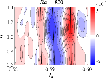
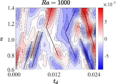
(c)                                                                    (d)

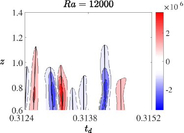
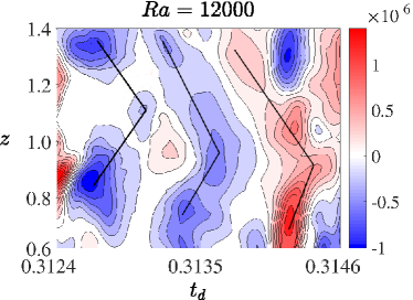
(e)                                                                    (f)

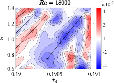
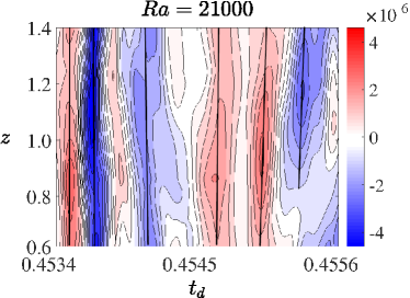
Figure 11: Contour plots of $\partial u_{z}/\partial t$ at cylindrical radius $s=0.3$ for small intervals of time in the saturated state. The parallel black lines indicate the predominant direction of travel of the waves and their slope gives the group velocity. The Rayleigh number $Ra$ of the simulation is given above each panel. The other dynamo parameters are $E=6\times 10^{-5},Pr=Pm=5$. The estimated group velocity of the fast and slow MAC waves ($U_{f}$ and $U_{s}$ respectively) and the measured group velocity $U_{g,z}$ are given in table 2.

In figure 11 , contours of $\partial u_{z}/\partial t$ are plotted for small time windows of approximately constant ambient magnetic field and wavenumbers at cylindrical radius $s=0.3$. The axial motion is measured by considering the full spectrum. In table 2, the measured axial group velocity of the waves, $U_{g,z}$ is compared with the estimated group velocity of the fast and slow MAC waves, given by $U_{f}$ and $U_{s}$ respectively. At $Ra=800$, convection is initiated within the TC under a weak ambient magnetic field. Consequently, only fast MAC waves are excited within the TC (figure 11(a)). At $Ra=1000$, the onset of slow MAC waves occurs (figure 11(b)); however, convection near the base of the TC is predominantly produced by the excitation of fast MAC waves (figure 11 (c)). At the location $(s,\phi)$ of the plume, the measured group velocity (figures 11 (b), (d) and (e)) matches well with that of the slow MAC waves. At the onset of polarity transitions, the slow waves disappear, and the homogeneous convection within the TC is entirely made up of fast waves (figure 11 (f)).

Figure 12 shows the fast Fourier transform (FFT) of $\partial u_{z}/\partial t$ separately for the lower ($0.6<z<1$) and upper ($1<z<1.5$) regions of the TC. The spectra were computed at discrete $\phi$ points and then azimuthally averaged. The thin vertical lines in figures 12 (a) and (b) give the values of $\omega_{s}^{\star}=\omega_{s}/\omega_{f}$, where $\omega_{f}$ and $\omega_{s}$ are the estimated frequencies of the fast and slow MAC waves. In the lower region of the TC, where the fast and slow waves coexist, the spectra suggest the dominance of the fast waves. However, the slow waves are dominant in the upper region of the TC. In the regime of polarity transitions ($Ra=21000$), the fast waves are dominant throughout the TC.

(a)                                                                    (b)

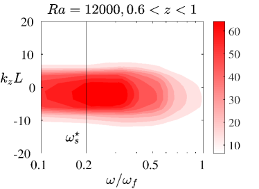
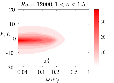
(c)                                                                    (d)

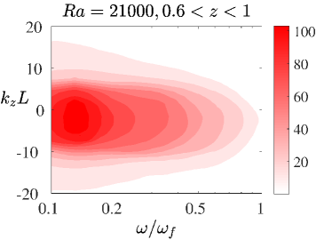
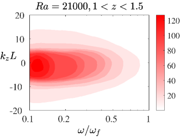
Figure 12: FFT spectra of $\partial u_{z}/\partial t$ for $0.6<z<1$ and $1<z<1.5$ inside tangent cylinder. The spectra are computed at discrete $\phi$ points and then averaged azimuthally from the saturated states of the dynamo runs. The thin vertical lines in (a) and (b) give $\omega_{s}^{\star}=\omega_{s}/\omega_{f}$, where $\omega_{f}$ and $\omega_{s}$ are the estimated fast and slow MAC wave frequencies. The Rayleigh number in the simulation is given above each panel. The other dynamo parameters are $E=6\times 10^{-5}$ and $Pm=Pr=5$.

Having understood from figures 11 and 12 that convection within the TC is made up of fast and slow MAC waves, we examine the magnitude of the wave motions in the neighbourhood of convective onset. In figure 13, the magnitude of the time-averaged peak $z$ velocity within the TC is plotted with respect to $z$ in two dynamo simulations near onset. At $Ra=800$, convection onsets via fast MAC waves, whose velocity does not change appreciably with $z$. At $Ra=1000$, the axial magnetic field concentrates within the TC, giving $|\omega_{M}/\omega_{C}|\approx 0.2$ (table 1). Here, the fast MAC wave velocity decreases appreciably in the region $z>1$, where the slow waves propagate as isolated plumes. Interestingly, the peak intensities of the fast and slow wave motions are approximately equal (see also table 3). The measurement of wave motions in the dynamo model enables meaningful comparisons of the dynamics within the TC with that predicted by linear magnetoconvection.

(a)                                                             (b)

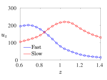
Figure 13: Variation of the time-averaged peak value of the axial ($z$) velocity with $z$ within the TC for (a) $Ra=800$ and (b) $Ra=1000$. The other dynamo parameters are $E=6\times 10^{-5},Pm=Pr=5$.

$Ra$	$Ra/Ra_{c}$	$N_{r}$	$l_{max}$	$Rm$	$Ro_{\ell}$	$\bar{k}_{\phi}$	$\bar{k}_{s}$	$\bar{k}_{z}$	$B^{2}_{peak}$	$B^{2}_{rms}$	$|\omega_{M}/\omega_{C}|$	$|\omega_{A}/\omega_{M}|$	$u_{\phi,\mbox{sc}}$
$E=6\times 10^{-5},Pm=Pr=5$
300	10.34	88	96	67	0.002	4.56	5.03	4.18	0.01	0.52	0.00	18.8	0.00 (0.00)
500	17.24	88	96	74	0.002	4.21	4.72	4.53	0.30	1.13	0.03	4.27	0.01 (0.02)
800	27.58	88	96	74	0.002	4.61	4.53	4.27	1.8	1.75	0.06	2.34	0.02 (0.07)
1000	34.48	128	120	98	0.004	4.14	4.12	4.48	26	2.48	0.21	0.67	0.08 (0.11)
2000	68.96	128	120	123	0.007	5.39	3.81	4.79	72	2.95	0.39	0.53	0.14 (0.11)
3000	103.45	160	160	169	0.009	6.21	3.97	4.72	112	3.26	0.55	0.53	0.15 (0.11)
6000	206.90	160	160	243	0.014	6.49	4.71	4.95	156	3.28	0.74	0.58	0.35 (0.11)
8000	275.86	160	180	288	0.020	6.34	4.58	5.96	180	3.29	0.73	0.55	0.41 (0.12)
12000	413.79	160	180	365	0.024	6.01	3.51	5.70	222	3.27	0.71	0.65	0.53 (0.15)
14000	482.76	160	180	402	0.026	5.87	4.09	5.13	227	3.18	0.76	0.75	0.65 (0.17)
16000	551.68	160	180	435	0.028	6.25	4.71	5.42	231	3.12	0.84	0.74	0.72 (0.18)
18000	620.69	160	180	456	0.032	6.59	4.53	5.30	234	3.04	0.88	0.79	0.81 (0.19)
20000	689.66	160	180	505	0.035	5.97	4.45	5.19	225	2.55	0.77	0.91	0.79 (0.20)
21000	724.14	160	180	549	0.039	6.21	4.17	5.24	65	0.62	0.43	1.63	0.19 (0.21)
$E=1.2\times 10^{-5},Pm=Pr=1$
300	10.34	90	96	78	0.004	4.07	2.89	4.76	0.01	0.31	0.00	18.4	0.00 (0.00)
700	24.14	90	96	102	0.005	4.71	3.76	5.11	0.69	2.11	0.03	3.13	0.01 (0.02)
1000	34.48	132	144	112	0.006	5.59	3.87	4.48	55	2.46	0.35	0.46	0.02 (0.03)
2500	86.21	168	160	174	0.011	5.37	4.14	5.30	90	3.59	0.44	0.49	0.08 (0.07)
4000	137.93	180	168	224	0.017	6.33	3.84	4.79	135	4.01	0.61	0.55	0.18 (0.11)
7000	241.38	192	180	312	0.026	6.35	4.04	5.58	194	4.69	0.72	0.53	0.34 (0.24)
10000	344.83	192	180	384	0.033	6.21	3.09	4.43	248	5.04	0.76	0.70	0.73 (0.32)
15000	517.24	192	180	500	0.045	7.21	3.79	4.70	260	5.35	0.88	0.79	0.78 (0.37)
20000	689.66	192	180	573	0.052	7.07	3.13	5.37	258	5.46	0.85	0.82	0.93 (0.45)
25000	862.07	192	180	655	0.061	7.67	3.03	5.34	255	5.84	0.90	0.93	1.07 (0.51)
27000	931.03	192	180	698	0.065	8.87	3.51	5.62	223	4.87	0.91	0.98	1.15 (0.50)
28000	965.52	192	180	775	0.073	8.82	3.39	5.76	89	0.82	0.62	1.52	0.31 (0.52)

Table 1: Summary of the main input and output parameters used in the dynamo simulations considered in this study. Here, $Ra$ is the modified Rayleigh number, $Ra_{c}$ is the critical Rayleigh number for the onset of nonmagnetic convection, $N_{r}$ is the number of radial grid points, $l_{max}$ is the maximum spherical harmonic degree, $Rm$ is the magnetic Reynolds number based on the shell thickness and $Ro_{l}$ is the local Rossby number. The mean $\phi$, $s$, and $z$ wavenumbers are denoted by $\bar{k}_{\phi}$, $\bar{k}_{s}$ and $\bar{k}_{z}$ respectively. In addition, $B^{2}_{peak}$ is the square of the peak field inside the TC in the saturated dynamo, $B^{2}_{rms}$ is the measured mean square value of the field in the spherical shell, and $u_{\phi,\mbox{sc}}$ is the scaled peak magnitude of the time and azimuthally averaged $\phi$ velocity inside the TC, with its nonmagnetic value given in brackets.

$Ra$	$\omega_{n}^{2}$	$\omega_{C}^{2}$	$\omega_{M}^{2}$	$-\omega_{A}^{2}$	$\omega_{f}$	$\omega_{s}$	$U_{f}$	$U_{s}$	$U_{g,z}$
	$(\times 10^{10})$	$(\times 10^{8})$	$(\times 10^{8})$	$(\times 10^{8})$	$(\times 10^{4})$	$(\times 10^{4})$
800	3.85	21.10	0.002	0.046	4.54	0	7543	0	7954
1000	3.21	23.27	2.00	0.51	5.16	0.331	7439	293	7141, 343
12000	1.27	27.87	11.59	6.75	5.98	1.22	6810	2051	8712, 1159
18000	1.53	21.94	19.39	10.42	6.76	1.95	7729	2477	8350, 1542
21000	0.53	22.86	3.82	11.17	4.50	0	7090	0	8927

Table 2: Summary of the data for MAC wave measurement in the dynamo models at $E=6\times 10^{-5},Pm=Pr=5$. The sampling frequency $\omega_{n}$ is chosen to ensure that the fast MAC waves are not missed in the measurement of group velocity. The values of $\omega_{C}^{2}$, $\omega_{M}^{2}$ and $-\omega_{A}^{2}$ are calculated using the mean values of $k_{\phi}$, $k_{s}$ and $k_{z}$. The measured group velocity in the $z$ direction ($U_{g,z}$) is compared with the estimated fast ($U_{f}$) or slow ($U_{s}$) MAC wave velocity.

3.3 Comparisons between the dynamo and linear magnetoconvection models

The TC may be approximated by a rotating layer in which convection takes place under an axial ($z$) magnetic field with gravity pointing in the downward $z$ direction. Therefore, a simplified linear model that studies the the evolution of a buoyancy disturbance in an unstably stratified rotating fluid under an axial magnetic field (figure 1) provides an insight into the role of wave motions in TC convection. The notable points of comparison between the linear and dynamo models are as follows:

1. Onset of slow MAC waves: The slow waves are detected within the TC when $|\omega_{M}/\omega_{C}|\sim 0.1$. This state is characterized by the approximate equality between the peak intensities of slow and fast waves (figure 13 (b) and table 3), in good agreement with the linear model where the two intensities match at $|\omega_{M}/\omega_{C}|\approx 0.2$ (figure 3 (c)). Furthermore, both models indicate that the parity between the wave motions persists for higher $\omega_{M}/\omega_{C}$.

2. Suppression of slow MAC waves under strong forcing: The slow wave velocity goes to zero within the TC when $|\omega_{A}/\omega_{M}|\approx 1$ (table 3), in agreement with the linear model (figure 3 (d)).

3. Intensity of polar vortices: For $|\omega_{M}/\omega_{C}|\sim 0.1$, the time and azimuthally averaged intensity of the polar vortex is much higher than that in nonmagnetic convection. However, when $|\omega_{A}/\omega_{M}|\approx 1$, the vortex intensity decreases appreciably to a value comparable to that in nonmagnetic convection (see figure 9 and table 1), in agreement with the behaviour of the toroidal kinetic energy in the linear model (figure 5).

$E=6\times 10^{-5},Pm=Pr=5$				$E=1.2\times 10^{-5},Pm=Pr=1$
$Ra$	$|\omega_{M}/\omega_{C}|$	$|\omega_{A}/\omega_{M}|$	$u_{z_{s}}^{\star}/u_{z_{f}}^{\star}$	$Ra$	$|\omega_{M}/\omega_{C}|$	$|\omega_{A}/\omega_{M}|$	$u_{z_{s}}^{\star}/u_{z_{f}}^{\star}$
1000	0.21	0.67	1.12	1000	0.35	0.46	1.23
2000	0.39	0.53	1.18	2500	0.44	0.49	1.31
3000	0.55	0.53	1.27	4000	0.61	0.55	1.28
18000	0.88	0.79	1.47	25000	0.90	0.93	1.44
20000	0.77	0.91	1.41	27000	0.91	0.98	1.46
21000	0.43	1.63	0	28000	0.62	1.52	0

Table 3: Ratio of the peak $z$ velocities of the slow and fast MAC waves, $u_{z,s}^{\star}/u_{z,f}^{\star}$, at progressively increasing forcing in two dynamo regimes considered in this study.

4 Concluding remarks

This study investigates convection within the tangent cylinder in rapidly rotating spherical dynamos through the analysis of forced MHD waves. Early studies (Sreenivasan and Jones, 2006) had shown that the polar vortices generated in the dynamo are considerably more intense than that in nonmagnetic convection due to the formation of isolated off-axis plumes within the TC. It was subsequently shown that convection would be localized by a laterally varying $z$ magnetic field (Sreenivasan and Gopinath, 2017), and the wavenumber at its onset would be determined by the Ekman number. The fact that the magnetic field confines convection suggests localized magnetostrophic balances within the TC. In this study, it is shown that slow MAC waves generated at the length scale of convection support the isolated TC upwellings in the dipole-dominated dynamo regime, in turn producing strong anticyclonic polar vortices. In regions where the magnetic flux is relatively weak, fast MAC waves are excited, although these waves are unable to penetrate the neutrally buoyant fluid layer that lies above them.

The observed secular variation of the Earth’s magnetic field (Olson and Aurnou, 1999; Hulot et al., 2002; Amit and Olson, 2006) suggests maximum drift rates of the polar vortex in the range 0.6–0.9^∘ yr^-1. The observed peak values are reached in the present low-inertia dynamo models for strongly driven convection with $Ra/Ra_{c}\sim 10^{3}$ (table 1). If the forcing is so strong as to cause polarity reversals, the field within the TC decays away, resulting in much weaker circulation in the polar regions.

Appendix A Equations for nonmagnetic convection

For $Pm=Pr$, the convection-driven dynamo given by equations (24)–(27) is compared with nonmagnetic convection given by the equations

$$EPr^{-1}\Bigl{(}\frac{\partial{\bm{u}}}{\partial t}+(\nabla\times{\bm{u}})\times{\bm{u}}\Bigr{)}+{\hat{\bm{z}}}\times{\bm{u}}=-\nabla p^{\star}+Ra\,T\,{\bm{r}}\,+E\nabla^{2}{\bm{u}},$$ (31)

$$\frac{\partial T}{\partial t}+({\bm{u}}\cdot\nabla)T=\nabla^{2}T,$$ (32)

$$\nabla\cdot{\bm{u}}=0,$$ (33)

where lengths are scaled by the thickness of the spherical shell $L$, time is scaled by $L^{2}/\kappa$, the velocity $\bm{u}$ is scaled by $\kappa/L$ and $p^{\star}=\frac{1}{2}EPr^{-1}|\bm{u}|^{2}$.

For a magnetic (dynamo) calculation with the parameters $E=6\times 10^{-5}$, $Pm=Pr=5$, $Ra=3000$, the equivalent non-magnetic calculation has the parameters $E=6\times 10^{-5}$, $Pr=5$, $Ra=3000$.

References

- Acheson and Hide (1973) Acheson, D.J., Hide, R., 1973. Hydromagnetics of rotating fluids. Rep. Prog. Phys. 36, 159.
- Amit and Olson (2006) Amit, H., Olson, P., 2006. Time-average and time-dependent parts of core flow. Phys. Earth Planet. Inter. 155, 120–139.
- Aujogue et al. (2018) Aujogue, K., Pothérat, A., Sreenivasan, B., Debray, F., 2018. Experimental study of the convection in a rotating tangent cylinder. J. Fluid Mech. 843, 355–381.
- Aurnou et al. (2003) Aurnou, J., Andreadis, S., Zhu, L., Olson, P., 2003. Experiments on convection in Earth’s core tangent cylinder. Earth Planet. Sci. Lett. 212, 119–134.
- Braginsky (1967) Braginsky, S.I., 1967. Magnetic waves in the earth’s core. Geomagn. Aeron. 7, 851–859.
- Braginsky and Roberts (1995) Braginsky, S.I., Roberts, P.H., 1995. Equations governing convection in Earth’s core and the geodynamo. Geophys. Astrophys. Fluid Dyn. 79, 1–97.
- Chandrasekhar (1961) Chandrasekhar, S., 1961. Hydrodynamic and Hydromagnetic Stability. Clarendon Press.
- Christensen and Aubert (2006) Christensen, U.R., Aubert, J., 2006. Scaling properties of convection-driven dynamos in rotating spherical shells and application to planetary magnetic fields. Geophys. J. Int. 166, 97–114.
- Gopinath and Sreenivasan (2015) Gopinath, V., Sreenivasan, B., 2015. On the control of rapidly rotating convection by an axially varying magnetic field. Geophys. Astrophys. Fluid Dyn. 109, 567–586.
- Hulot et al. (2002) Hulot, G., Eymin, C., Langlais, B., Mandea, M., Olsen, N., 2002. Small-scale structure of the geodynamo inferred from Oersted and Magsat satellite data. Nature 416, 620–623.
- Jones (2015) Jones, C.A., 2015. Thermal and compositional convection in the outer core, in: Olson, P. (Ed.), Treatise on Gephysics. Elsevier. volume 8, pp. 115–159.
- Jones et al. (2003) Jones, C.A., Mussa, A.I., Worland, S.J., 2003. Magnetoconvection in a rapidly rotating sphere: the weak-field case. Proc. R. Soc. Lond. A 459, 773–797.
- Majumder et al. (2023) Majumder, D., Sreenivasan, B., Maurya, G., 2023. Self-similarity of the dipole–multipole transition in rapidly rotating dynamos. J. Fluid Mech. , http://arxiv.org/abs/2305.17640 (in revision).
- Olson and Aurnou (1999) Olson, P., Aurnou, J., 1999. A polar vortex in the Earth’s core. Nature 402, 170–173.
- Schaeffer et al. (2017) Schaeffer, N., Jault, D., Nataf, H.C., Fournier, A., 2017. Turbulent geodynamo simulations: a leap towards Earth’s core. Geophys. J. Int. 211, 1–29.
- Sreenivasan and Gopinath (2017) Sreenivasan, B., Gopinath, V., 2017. Confinement of rotating convection by a laterally varying magnetic field. J. Fluid Mech. 822, 590–616.
- Sreenivasan and Jones (2005) Sreenivasan, B., Jones, C.A., 2005. Structure and dynamics of the polar vortex in the Earth’s core. Geophys. Res. Lett. 32.
- Sreenivasan and Jones (2006) Sreenivasan, B., Jones, C.A., 2006. Azimuthal winds, convection and dynamo action in the polar regions of planetary cores. Geophys. Astrophys. Fluid Dyn. 100, 319–339.
- Sreenivasan and Maurya (2021) Sreenivasan, B., Maurya, G., 2021. Evolution of forced magnetohydrodynamic waves in a stratified fluid. J. Fluid Mech. 922, A32.
- Sreenivasan and Narasimhan (2017) Sreenivasan, B., Narasimhan, G., 2017. Damping of magnetohydrodynamic waves in a rotating fluid. J. Fluid Mech. 828, 867–905.
- Varma and Sreenivasan (2022) Varma, A., Sreenivasan, B., 2022. The role of slow magnetostrophic waves in the formation of the axial dipole in planetary dynamos. Phys. Earth Planet. Inter. 333, 106944.
- Willis et al. (2007) Willis, A.P., Sreenivasan, B., Gubbins, D., 2007. Thermal core–mantle interaction: exploring regimes for ‘locked’ dynamo action. Phys. Earth Planet. Inter. 165, 83–92.
- Zhang (1995) Zhang, K., 1995. Spherical shell rotating convection in the presence of a toroidal magnetic field. Proc. R. Soc. Lond. A 448, 243–268.