Accounting for localized deformation: a simple computation of true stress in micropillar compression experiments

Abstract

Compression experiments are widely used to study the mechanical properties of materials at micro- and nanoscale. However, the conventional engineering stress measurement method used in these experiments neglects to account for the alterations in the material’s shape during loading. This can lead to inaccurate stress values and potentially misleading conclusions about the material’s mechanical behavior, especially in the case of localized deformation. To address this issue, we present a method for calculating true stress in cases of localized plastic deformation commonly encountered in experimental settings: (i) a single band and (ii) two bands oriented in arbitrary directions with respect to the vertical axis of the pillar (either in the same or opposite directions). Our simple analytic formulas can be applied to homogeneous and isotropic materials and crystals, requiring only standard data (displacement-force curve, aspect ratio, shear band angle and elastic strain limit) obtained from experimental results and eliminating the need for finite element computations. Our approach provides a more precise interpretation of experimental results and can serve as a valuable and simple tool in material design and characterization.

I Introduction

Compression experiments conducted on pillars have proven to be a valuable method for analyzing the mechanical behavior of materials at the micro- and nano-scales. This approach involves the fabrication of micro-pillars (often with focused ion beam (FIB) techniques) followed by an uni-axial compression to study its mechanical response in a strain-driven process. This method has been particularly useful for investigating the onset and evolution of plastic deformation in materials, by exploring the local deformation mechanism (when compression test are carried out in situ SEM), see for instance Uchic et al. (2004); Greer et al. (2005); Ng and Ngan (2008); Frick et al. (2008); Kiener et al. (2011); Friedman et al. (2012); Zhang et al. (2017a); Salman and Ionescu (2021); Zhang et al. (2020); Salman et al. (2021); Cui et al. (2021). Specifically, micro-pillar compression experiments have revealed numerous new phenomena, including the transition from wild-to-mild plasticity Zhang et al. (2017a), pristine-to-pristine plastic deformation Wang et al. (2012), the ”smaller is stronger” effect Lee et al. (2009), size- and shape-dependent flow stresses Uchic et al. (2004); Maaß et al. (2012); Zhang et al. (2017b) and, microstructural control of plastic flow Rizzardi et al. (2022), among others.

During such compression experiments, the material can undergo significant plastic deformation, which can manifest in either homogeneous deformation or slip/kink bands Hagihara et al. (2016); Mayer et al. (2016); Basak et al. (2019); Chen et al. (2020); Nandam et al. (2021); Weiss et al. (2021); Nizolek et al. (2021); Marano et al. (2021); Zhang et al. (2022). Homogeneous deformation occurs when the material undergoes uniform deformation throughout its structure, while slip/kink bands result from localized deformation that can form along some preferred orientation Inamura (2019); Gan et al. (2020). The resulting engineering strain-stress curve is related to a displacement-force experimental recording, but in order to accurately characterize the material’s mechanical behavior, it is necessary to determine the Eulerian (true) stress that is exerted within the deformation zone. It is especially crucial to be able to accurately interpret the mechanical properties of engineered or designed materials using various methods to assess whether desired enhancements have been achieved Wu et al. (2021); Ghidelli et al. (2021). The significance of using true stress in assessing mechanical responses has been discussed in prior studies related to the mechanical behavior of metallic glass Han et al. (2008); Wang et al. (2017). However, of particular importance is the fact that, to the best of our knowledge, there is currently no established method to calculate the required load-bearing area to evaluate true stress, during plastic localization mechanisms.

In this context, the aim of this study is to derive simple formulas for calculating true stress in cases involving slip/kink band formation during mechanical loading while avoiding the need for lengthy and complex finite element computations that deal with large deformations of crystals. Specifically, we consider different scenarios of localization observed frequently in experiments: (i) a single band and (ii) two bands oriented in arbitrary directions with respect to the vertical axis of the pillar. For each case, we derive a formula and employ it to assess the reliability of previous experimental results.

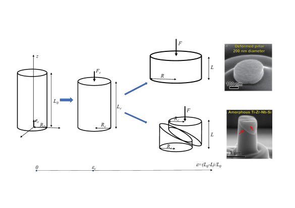
Figure 1: Schematic representation of the nano or micro-pillar deformation. The linear elastic regime, $\epsilon^{eng}<\epsilon_{e}$, is followed by one of the two types of plastic flow. Up: homogeneous deformation, Bottom: shear/kick band deformation (experimental illustration taken from Wu et al. (2021)).

II Simple modeling of pillars’ deformation

After the initial loading process, which is associated with small-strain linear elastic behavior, the pillars undergo significant plastic deformation, making the elastic deformations negligible in comparison to the plastic ones. From these plastic deformation processes, two distinct scenarios emerge: homogeneous and slip/kink band, as illustrated schematically in Figure 1 and detailed subsequently. The Cauchy stress tensors corresponding to these two deformation mechanisms exhibit different patterns. In either scenario, the primary challenge is to determine the true stress $\sigma^{true}$ within the uniaxial Cauchy stress tensor ${\boldsymbol{\sigma}}=-\sigma^{true}{\boldsymbol{e}}_{z}\otimes{\boldsymbol{e}}_{z}$, where ${\boldsymbol{e}}_{i}$ represents the elements of the orthonormal basis of the three-dimensional Euclidean vector space, acting on the active area $A_{u}$.

To be more specific, let $R_{0}$ and $L_{0}$ represent the initial (Lagrangian) radius and height of the cylindrical pillar, respectively, while $R$ and $L$ denote the current (Eulerian) dimensions during deformation, as shown in Fig. 1. Let $\epsilon^{eng}=(L_{0}-L)/L_{0}$ denote the overall engineering strain. Let ${\boldsymbol{F}}=-F{\boldsymbol{e}}_{z}$ represent the force applied to the top of the pillar during deformation, where $F=\sigma^{true}A_{u}$, and let $\sigma^{eng}$denote the nominal (engineering) stress, i.e., $F=\sigma^{eng}A_{0}$, with $A_{0}=\pi R_{0}^{2}$ is the original cross-sectional area.

We assume knowledge of the initial pillar shape, specifically the aspect ratio $f_{0}=L_{0}/2R_{0}$, and have access to the engineering strain-stress curve, denoted as the function $\epsilon^{eng}\to\sigma^{eng}(\epsilon^{eng})$. The primary objective of this paper is to derive a simple formula for estimating the engineering strain-true stress curve, represented as $\epsilon^{eng}\to\sigma^{true}(\epsilon^{eng})$.

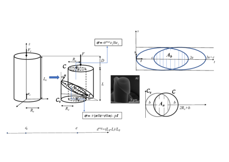
Figure 2: (Left): Schematic representation of localized plastic deformation following the elastic stage with the Cauchy stress tensor acting in different regions of the pillar. (Right, top): The plan of the shear band with its area $A_{b}$ between two ellipses representing the upper and lower sections of the pillar. (Right, bottom) : Its projection on the horizontal plane (experimental image taken from Weiss et al. (2021)).

Elastic deformation

For $\epsilon^{eng}<\epsilon_{e}$ (or equivalently for $\sigma^{eng}<\sigma^{eng}_{e}$) the pillar exhibits a linear elastic behavior. Here, $\epsilon_{e}$ and $\sigma^{eng}_{e}=\sigma^{eng}(\epsilon_{e})$ represent the strain and stress limits of elasticity, which can be easily identified in each stress-strain (or force-displacement) curve. Since the elastic strain limit $\epsilon_{e}$, is usually small (less that $3\%$) the elastic linear theory can be accepted as a good approximation. For isotropic materials, the deformed shape is also a cylinder, and the stress is uniaxial throughout the pillar: $A_{u}=A=\pi R^{2},F=\sigma^{true}\pi R^{2}$ and $\sigma^{eng}R_{0}^{2}=\sigma^{true}R^{2}$. For anisotropic materials, such as monocrystals, during the elastic phase, the pillar is no longer a perfect cylinder. However, since the deformation is small, the deviation from a cylindrical shape can be neglected.

For small values of $\delta_{e}=\sigma^{eng}_{e}/3K$ (where $K$ is the bulk modulus) and $\epsilon_{e}$, the formula for true stress is well-known:

$$\sigma^{true}=\sigma^{eng}(1-\epsilon^{eng}),\quad\quad\mbox{for}\;\epsilon^{eng}\leq\epsilon_{e}.$$ (1)

Note that since $1-\epsilon^{eng}\approx 1$ for $\epsilon^{eng}<\epsilon_{e}$ the difference between the true and engineering stress in not significant, and we can conclude that $\sigma^{true}\approx\sigma^{eng}$ during the elastic phase.

Homogeneous uni-axial stress

For larger deformations, $\epsilon^{eng}>\epsilon_{e}$, in the first scenario the deformation is homogeneous and the stress throughout the entire pillar is assumed to be uni-axial, given by ${\boldsymbol{\sigma}}=-\sigma^{true}{\boldsymbol{e}}_{z}\otimes{\boldsymbol{e}}_{z}$, where $A_{u}=A=\pi R^{2}$. For materials modeled by a pressure-independent plasticity law, plastic deformation is isochoric and the volume is preserved. In the case of isotropic materials, the deformed shape remains a cylinder, and since the further elastic deformation of the volume can be neglected we have $V=\pi R^{2}L=V_{e}=\pi R_{e}^{2}L_{e}$, where $R_{e}$ and $L_{e}$ are the radius and length of the pillar at the end of the elastic phase. After some algebra we find the well known formula

$$\sigma^{true}=\sigma^{eng}(1-\epsilon^{eng}),\quad\mbox{for}\;\epsilon^{eng}>\epsilon_{e}.$$ (2)

However, for large values of $\epsilon^{eng}$, using the nominal stress $\sigma^{eng}$ instead of the Cauchy stress $\sigma^{true}$ can significantly alter the behavior of the stress-strain diagram, giving a false impression of overall hardening-like behavior.

Single slip/kink band plastic deformation

In the second scenario, for $\epsilon^{eng}>\epsilon_{e}$, deformation is localized in a narrow zone between two parallel planes with a normal vector ${\boldsymbol{n}}$, determined by the angle $\alpha$ with respect to the vertical axis ${\boldsymbol{e}}_{z}$, see Fig. 2. The Cauchy stress tensor acting in the shear band is given by ${\boldsymbol{\sigma}}=\tau({\boldsymbol{n}}\otimes{\boldsymbol{t}}+{\boldsymbol{t}}\otimes{\boldsymbol{n}})-p{\boldsymbol{I}}$, where ${\boldsymbol{t}}$ is the slip direction, $\tau$ is the shear stress and, ${\boldsymbol{I}}$ is the identity matrix. Since the Cauchy stress tensor acting in the regions above and below the shear band is assumed to be uniaxial, i.e., ${\boldsymbol{\sigma}}=\sigma^{true}{\boldsymbol{e}}_{z}\otimes{\boldsymbol{e}}_{z}$, we can deduce that the expression for the shear stress $\tau$, acting in the shear band, is proportional to the true stress:

$$\tau=\frac{1}{2}\sin(2\alpha)\sigma^{true}.$$ (3)

Let us now compute the area $A_{u}$ between the two disks (or equivalently $A_{b}=A_{u}/\cos(\alpha)$ the area between the two ellipses) ${\cal C}_{e}$ and $\cal{C}$ corresponding to the projection on the basal plane of the two cylinders (see Fig. 2). One of the circles is translated by a distance of $b=D\cot(\alpha)$, where $D=L_{e}-L$ is the vertical displacement of the upper pillar region. After some simple computations, one can find that the area $A_{u}$ between the two regions is given by

$$A_{u}=R_{e}^{2}\left[\pi-\frac{b}{R_{e}}\sqrt{1-\frac{b^{2}}{4R_{e}^{2}}}-2\arcsin\left(\frac{b}{2R_{e}}\right)\right].$$

Denoting by $f_{0}=L_{0}/2R_{0}$ the initial shape number and by $f_{e}=L_{e}/2R_{e}=(1-\epsilon_{e})^{3/2}f_{0}$ the shape number at the end of the elastic phase, and by $\epsilon_{*}^{eng}=(L-L_{e})/L_{e}=(\epsilon^{eng}-\epsilon_{e})/(1+\epsilon_{e})$ the engineering (plastic) deformation with respect to the configuration at the end of the elastic phase, we get

$$A_{u}=R_{e}^{2}\Phi(\epsilon_{*}^{eng}f_{e}\cot(\alpha)),$$ (4)

where we have denoted by

$$\Phi(s)=\pi-2s\sqrt{1-s^{2}}-2\arcsin(s).$$

Taking into account that $R_{0}^{2}/R_{e}^{2}=(1-\sqrt{1-4\delta_{e}(1-\epsilon_{e})})/2\delta_{e}$ we can deduce that:

$$\sigma^{true}=\frac{\sigma^{eng}\pi(1-\sqrt{1-4\delta_{e}(1-\epsilon_{e})})}{2\delta_{e}\Phi((\epsilon^{eng}-\epsilon_{e})/(1+\epsilon_{e})f_{e}\cot(\alpha))},$$ (5)

for $\epsilon^{eng}>\epsilon_{e}$.

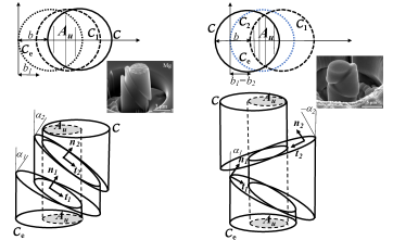
Figure 3: Schematic representation of localized plastic deformation: two localized bands with two different orientation angles: (left) $\alpha_{1},\alpha_{2}>0$; (right) $\alpha_{1}>0>-\alpha_{2}$. Insets are taken from the experiments in Weiss et al. (2021). In the upper part, we plot the projection on the horizontal plane of the bands with their area $A_{u}$ at different stages of localization.

For small values of $\epsilon_{e}$ and $\delta_{e}$, we have $R_{0}^{2}/R_{e}^{2}\approx 1-\epsilon_{e}$, $f_{e}\approx f_{0}$, and the plastic deformation reads $\epsilon_{*}^{eng}\approx\epsilon^{eng}-\epsilon_{e}$. We can deduce a simplified formula for the true stress:

$$\sigma^{true}=\frac{\pi(1-\epsilon_{e})\sigma^{eng}}{\Phi(s)},$$ (6)

where $s$ is given by

$$s=(\epsilon^{eng}-\epsilon_{e})f_{0}\cot(\alpha),\quad\mbox{for}\;\epsilon^{eng}>\epsilon_{e}.$$ (7)

Note that to use the simplified formula we only need to know the elastic limit $\epsilon_{e}$, the shear band angle $\alpha$ and the initial aspect ratio $f_{0}$. However, the exact formula given in Eq. 5 requires also $\delta_{e}$: the ratio between engineering stress $\sigma^{eng}_{e}$ at the end of the elastic phase and the bulk modulus $K$.

In contrast to the homogeneous deformation scenario, here the true stress is larger than the engineering stress. Therefore, in many strain-stress diagrams, the plateau or softening of the engineering stress should be viewed as a hardening of the true stress.

It should also be noted that combining the above formula with equation (3) allows for the calculation of the shear stress $\tau$ as a function of the shear plastic strain $\gamma_{p}$, which can be expressed as

$$\gamma_{p}=\frac{L_{e}-L}{\cos(\alpha)H_{b}}=\frac{(\epsilon^{eng}-\epsilon_{e})L_{0}}{\cos(\alpha)H_{b}},$$

where $H_{b}$ represents the thickness of the shear band. Note the plastic shear strain $\gamma_{p}$ is proportional with the plastic axial engineering strain $\epsilon^{eng}_{p}=\epsilon^{eng}-\epsilon_{e}$.

Multiple slip/kink band plastic deformation

It is worth noting that in certain experiments, the formation of multiple shear or kink bands is frequently observed Guo et al. (2016); Zhang et al. (2020); Weiss et al. (2021). To account for the presence of these additional bands we shall use a similar approach, as described above. Since the analysis becomes significantly more complex we shall suppose, as is depicted in Fig. 3, that we deal with only two shear bands $({\boldsymbol{n}}_{1},{\boldsymbol{t}}_{1})$ and $({\boldsymbol{n}}_{2},{\boldsymbol{t}}_{2})$ with co-planar slipping systems (i.e. ${\boldsymbol{n}}_{1}\wedge{\boldsymbol{t}}_{1}={\boldsymbol{n}}_{2}\wedge{\boldsymbol{t}}_{2}$). We shall also suppose that the shear band $({\boldsymbol{n}}_{1},{\boldsymbol{t}}_{1})$ becomes inactive at $\epsilon^{eng}=\epsilon^{eng}_{1}$ (corresponding to circle ${\cal C}_{1}$ at the distance $b_{1}=D_{1}\cot(\alpha_{1})$ from circle ${\cal C}_{e}$) when the slip starts on the shear band $({\boldsymbol{n}}_{2},{\boldsymbol{t}}_{2})$. Notice that for $\epsilon^{eng}<\epsilon^{eng}_{1}$ we deal with a single slip system and the simplified formula (6-7) is still valid. For $\epsilon^{eng}>\epsilon^{eng}_{1}$ we need to distinguish two cases: when the orientation angles of the two shear bands have the same sign ($\alpha_{1},\alpha_{2}>0$ as shown in Fig. 3 on the left) or when they have opposite signs ($-\alpha_{2}<0<\alpha_{1}$ as shown in Fig. 3 on the right).

In the first case, depicted in Fig. 3 on the left, for $\epsilon^{eng}>\epsilon^{eng}_{1}$ the intersection of three cylinders’ projections on the basal plane is the intersection of circle ${\cal C}$ with ${\cal C}_{e}$ at the distance $b=b_{1}+(D-D_{1})\cot(\alpha_{2})$. In the simplified formula (6), the variable $s$ is computed as follows:

$$s=f_{0}(\epsilon^{eng}-\epsilon_{e})\cot(\alpha_{1})\;\quad\mbox{for}\;\quad\epsilon^{eng}\in[\epsilon_{e},\epsilon^{eng}_{1}],$$ (8)

$$s=f_{0}((\epsilon^{eng}_{1}-\epsilon_{e})\cot(\alpha_{1})+(\epsilon^{eng}-\epsilon^{eng}_{1})\cot(\alpha_{2})),$$ (9)

for $\epsilon^{eng}\geq\epsilon^{eng}_{1}$. We remark that if the two shear bands have the same slope $\alpha_{1}=\alpha_{2}=\alpha$, then the formula (6) is still valid.

In the second case, depicted on the right in Fig. 3, we remark that for $\epsilon^{eng}>\epsilon^{eng}_{1}$ the projection ${\cal C}$ of the upper cylinder on the basal plane is in the opposite direction. Hence, in a first phase, when the circle ${\cal C}$ is approaching to ${\cal C}_{e}$ and the distance $b$ between ${\cal C}$ and ${\cal C}_{1}$ is less than $b_{1}$, the intersection of three cylinders’ projections does not change (i.e., it remains the intersection of ${\cal C}_{e}$ and ${\cal C}_{1}$). This phase ends when ${\cal C}$ coincides with ${\cal C}_{e}$, i.e. when $\epsilon^{eng}=\epsilon^{eng}_{2}$, where we have denoted by

$$\epsilon^{eng}_{2}=\epsilon^{eng}_{1}+(\epsilon^{eng}_{1}-\epsilon_{e})\cot(\alpha_{1})/\cot(\alpha_{2}).$$

For $\epsilon^{eng}>\epsilon^{eng}_{2}$ the intersection of the projections of the three cylinders becomes the intersection of ${\cal C}$ and ${\cal C}_{1}$. Then in the simplified formula (6) $s$ reads as (8) for $\epsilon^{eng}\in[\epsilon_{e},\epsilon^{eng}_{1}]$, and

$$s=f_{0}(\epsilon^{eng}_{1}-\epsilon_{e})\cot(\alpha_{1}),\;\mbox{for}\;\epsilon^{eng}\in[\epsilon^{eng}_{1},\epsilon^{eng}_{2}],$$ (10)

while for $\epsilon^{eng}>\epsilon^{eng}_{2}$ we have

$$s=f_{0}((\epsilon^{eng}_{1}-\epsilon_{e})\cot(\alpha_{1})+(\epsilon^{eng}-\epsilon^{eng}_{2})\cot(\alpha_{2})).$$ (11)

It’s worth noting that in the second case there exists a plateau $[\epsilon^{eng}_{1},\epsilon^{eng}_{2}]$ during which the effective area does not decrease ($s$ is constant in (10)).

Note that in the case of multiple shear bands, the true stress formulas (8-11) require, in addition to the single-band case (6), only the value of the strain $\epsilon^{eng}_{1}$ associated with the beginning of the second shear band formation.

III True stress computation and re-interpretation of the stress-strain curves

In this section, we want to illustrate how the formulas deduced in the previous section alter some experimental engineering strain-stress curves reported in the literature. We consider one case of homogeneous plastic deformation and three cases of localized plastic deformation: a single band, two bands with orientation angles having the same sign ($\alpha_{1},\alpha_{2}>0$), and opposite signs ($-\alpha_{2}<0<\alpha_{1}$).

Homogeneous and single slip/kink band plastic deformation

As a first example, we will reconsider the strain-stress behavior of a crystal-glass symbiotic alloy investigated in Wu et al. (2021). In this study, the authors plotted the engineering strain-stress curves to characterize the crystal-glass nano-laminated alloy sample’s mechanical properties compared with its crystalline and amorphous counterparts. Interestingly, the authors found that the nano-laminated crystal-glass alloy appeared to be tougher than its individual components when analyzing the engineering stress data (see Fig. 4(a) in Wu et al. (2021)). However, when we calculate the engineering strain vs. true stress curves for two cases: (i) the crystal-glass nano-laminated alloy undergoing homogeneous deformation using the conventional formula provided in Eq. (2); (ii) the CrCoNi crystal experiencing slip band deformation using Eq. 5 (or the simplified formula given in Eqs. 6-7), we observe a contradictory outcome in both cases. Specifically, the nano-laminated alloy exhibits softening, as shown in Fig. 4(a), while the CrCoNi crystal demonstrates hardening, as depicted in Fig. 4(b). This finding emphasizes the significance of taking into account the current deformation state of the material, even in the absence of a strong localization.

Lastly, we emphasize that when comparing the true stress curves obtained using Eq. (5) and the simplified formulas provided in Eqs. (6-7), as shown in Fig. 4(b), we observed minimal differences, even at high strains. Consequently, we will exclusively utilize the simplified formulations in the following example.

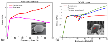
Figure 4: Engineering strain vs. nominal stress (red) and true stress (blue) curves. Nominal stress values are taken from Wu et al. (2021)) and the calculated true stress curves are calculated using the formulas derived here. (a) homogeneous deformation of a crystal-glass nano-laminated alloy sample calculated with the classical formulas (1), (2); (b) single shear band deformation of a CrCoNi crystal calculated with formulas (1), (5) (blue) and simplified formula (6-11) (green). Here, we took $\alpha=\pi/4$, $f_{0}=$1$,\varepsilon_{e}=$2.5% and $\sigma^{eng}_{e}=$3.23 GPa. Insets show the final state of the pillar at the end of the loading.

Multiple slip/kink band plastic deformation

In our second example, we illustrate two cases of multiple shear bands. One is constructed from magnesium, featuring a hexagonal close-packed (HCP) crystal lattice symmetry and possessing a radius of $3500$ nm. The other pillar is made of aluminum, exhibiting a face-centered cubic (FCC) symmetry and having a radius of $6000$ nm. In the case of the magnesium pillar, we observe the emergence of two shear bands oriented in the same direction ($\alpha_{1},\alpha_{2}>0$), while in the aluminum pillar, two shear bands are oriented such that $-\alpha_{2}<0<\alpha_{1}$, as depicted in the insets in Fig. 3, see also Weiss et al. (2021). The experimental engineering strain-stress curves for magnesium and aluminum, displayed in Figs. 5(a,b), are plotted in red. It’s important to note that the stress values in both cases represent engineering stress and do not account for the current shape of the pillars. We then apply Eqs. (6) (8-11) (for the first case we used $\alpha_{1}=\alpha_{2}=\pi/4$, $f_{0}=$1, $\varepsilon_{e}=$1.7% and $\varepsilon_{1}=$7%, while for the second we take $\alpha_{1}=\alpha_{2}=\pi/4$, $f_{0}=$1, $\varepsilon_{e}=$0.9% and $\varepsilon_{1}=$9%) to obtain the true-stress curves, which are shown in Fig. 5 in blue.

We observe that when examining the stress-strain of the magnesium pillar in Fig. 5(a), strain-hardening becomes evident after a 10 percent deformation, a phenomenon not observable when using engineering stress measurements.

In the case of the aluminum pillar, however, the overall qualitative trend is similar in both engineering and true stresses, i.e., an almost flat regime between 2-10 percent deformation followed by a strain-hardening regime. This is due to the fact that the slips on the shear bands are in opposite directions. Indeed, in this case, as it follows from (10), the ratio between the engineering and true stresses is constant for a large strain interval $[\epsilon^{eng}_{1},\epsilon^{eng}_{2}]$. The main difference is primarily quantitative in stress values, which are slightly larger when true stress is used.

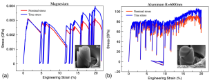
Figure 5: Comparison of engineering strain vs. nominal stress (red) and true stress (blue) curves. The nominal stress values are taken from Weiss et al. (2021)) and the true stress values are calculated using the simplified formulas (1),(6), (8-11). (a) Magnesium sample featuring two bands with $\alpha_{1},\alpha_{2}>0$. (b) Aluminum with featuring two bands oriented such that $-\alpha_{2}<0<\alpha_{1}$. Insets show final state of the pillar at the end of the loading.

IV Conclusion

In conclusion, our study provides formulas for calculating true stress in cases where slip/kink bands form during mechanical loading in compression experiments on pillars. These formulas are very simple and need only the engineering stress data, some geometric data (aspect ratio), and some mechanical data (elastic limit) which are very simple to get from the experimental results. A more precise alternative to these simple formulas could be very long and difficult finite element computations involving large deformation of crystals. However, using these formulas, we re-evaluated the robustness of previous experimental results and found that considering the current deformation state of engineered materials can be important for accurately interpreting their mechanical behavior at small scales. To be more precise, our analysis revealed that, in some cases, the true stress led to conclusions that were exactly opposite to those found using the engineering stress, while in other cases, the difference is mainly quantitative and the overall trend is similar. To conclude, our work provides a valuable tool for accurately interpreting the mechanical behavior of materials under compressive loads and for drawing appropriate conclusions based on the true stress values.

Acknowledgments

O.U.S. is supported by the grants ANR-18-CE42-0017-03, ANR-19-CE08-0010-01, ANR-20-CE91-0010, M.G. is supported by the grant ANR-21-CE08-0003-01 and I.I. acknowledges the support of the Romanian Ministry of Research (PN-III-P4-PCE-2021-0921 within PNCDI III).

References

- Uchic et al. (2004) M. D. Uchic, D. M. Dimiduk, J. N. Florando, and W. D. Nix, Science 305, 986 (2004).
- Greer et al. (2005) J. R. Greer, W. C. Oliver, and W. D. Nix, Acta Mater. 53, 1821 (2005).
- Ng and Ngan (2008) K. S. Ng and A. H. W. Ngan, Acta Mater. 56, 1712 (2008).
- Frick et al. (2008) C. P. Frick, B. G. Clark, S. Orso, A. S. Schneider, and E. Arzt, Materials Science and Engineering: A 489, 319 (2008).
- Kiener et al. (2011) D. Kiener, P. J. Guruprasad, S. M. Keralavarma, G. Dehm, and A. A. Benzerga, Acta Mater. 59, 3825 (2011).
- Friedman et al. (2012) N. Friedman, A. T. Jennings, G. Tsekenis, J.-Y. Kim, M. Tao, J. T. Uhl, J. R. Greer, and K. A. Dahmen, Phys. Rev. Lett. 109, 095507 (2012).
- Zhang et al. (2017a) P. Zhang, O. U. Salman, J.-Y. Zhang, G. Liu, J. Weiss, L. Truskinovsky, and J. Sun, Acta Mater. 128, 351 (2017a).
- Salman and Ionescu (2021) O. U. Salman and I. R. Ionescu, Mech. Res. Commun. 114, 103665 (2021).
- Zhang et al. (2020) P. Zhang, O. U. Salman, J. Weiss, and L. Truskinovsky, Phys Rev E 102, 023006 (2020).
- Salman et al. (2021) O. U. Salman, R. Baggio, B. Bacroix, G. Zanzotto, N. Gorbushin, and L. Truskinovsky, C. R. Phys. 22, 1 (2021).
- Cui et al. (2021) Y. Cui, E. Aydogan, J. G. Gigax, Y. Wang, A. Misra, S. A. Maloy, and N. Li, Acta Mater. 202, 255 (2021).
- Wang et al. (2012) Z.-J. Wang, Z.-W. Shan, J. Li, J. Sun, and E. Ma, Acta Mater. 60, 1368 (2012).
- Lee et al. (2009) S.-W. Lee, S. M. Han, and W. D. Nix, Acta Mater. 57, 4404 (2009).
- Maaß et al. (2012) R. Maaß, L. Meza, B. Gan, S. Tin, and J. R. Greer, Small 8, 1869 (2012).
- Zhang et al. (2017b) J. Zhang, K. Kishida, and H. Inui, Int. J. Plast. 92, 45 (2017b).
- Rizzardi et al. (2022) Q. Rizzardi, P. M. Derlet, and R. Maaß, Phys. Rev. Mater. 6, 073602 (2022).
- Hagihara et al. (2016) K. Hagihara, T. Mayama, M. Honnami, M. Yamasaki, H. Izuno, T. Okamoto, T. Ohashi, T. Nakano, and Y. Kawamura, Int. J. Plast. 77, 174 (2016).
- Mayer et al. (2016) C. R. Mayer, L. W. Yang, S. S. Singh, J. Llorca, J. M. Molina-Aldareguia, Y. L. Shen, and N. Chawla, Acta Mater. 114, 25 (2016).
- Basak et al. (2019) A. K. Basak, A. Pramanik, and C. Prakash, Materials Science and Engineering: A 763, 138141 (2019).
- Chen et al. (2020) M. Chen, L. Pethö, A. S. Sologubenko, H. Ma, J. Michler, R. Spolenak, and J. M. Wheeler, Nat. Commun. 11, 2681 (2020).
- Nandam et al. (2021) S. H. Nandam, R. Schwaiger, A. Kobler, C. Kübel, C. Wang, Y. Ivanisenko, and H. Hahn, J. Mater. Res. 36, 2903 (2021).
- Weiss et al. (2021) J. Weiss, P. Zhang, O. U. Salman, G. Liu, and L. Truskinovsky, C. R. Phys. 22, 1 (2021).
- Nizolek et al. (2021) T. J. Nizolek, T. M. Pollock, and R. M. McMeeking, J. Mech. Phys. Solids 146, 104183 (2021).
- Marano et al. (2021) A. Marano, L. Gélébart, and S. Forest, J. Mech. Phys. Solids 149, 104295 (2021).
- Zhang et al. (2022) Y. Zhang, N. Li, M. M. Schneider, T. J. Nizolek, L. Capolungo, and R. J. McCabe, Acta Mater. 237, 118150 (2022).
- Inamura (2019) T. Inamura, Acta Mater. 173, 270 (2019).
- Gan et al. (2020) K. Gan, S. Zhu, S. Jiang, and Y. Huang, J. Alloys Compd. 831, 154719 (2020).
- Wu et al. (2021) G. Wu, C. Liu, A. Brognara, M. Ghidelli, Y. Bao, S. Liu, X. Wu, W. Xia, H. Zhao, J. Rao, D. Ponge, V. Devulapalli, W. Lu, G. Dehm, D. Raabe, and Z. Li, Mater. Today 51, 6 (2021).
- Ghidelli et al. (2021) M. Ghidelli, A. Orekhov, A. L. Bassi, G. Terraneo, P. Djemia, G. Abadias, M. Nord, A. Béché, N. Gauquelin, J. Verbeeck, J.-P. Raskin, D. Schryvers, T. Pardoen, and H. Idrissi, Acta Mater. 213, 116955 (2021).
- Han et al. (2008) Z. Han, H. Yang, W. F. Wu, and Y. Li, Appl. Phys. Lett. 93, 231912 (2008).
- Wang et al. (2017) J. G. Wang, Y. C. Hu, P. F. Guan, K. K. Song, L. Wang, G. Wang, Y. Pan, B. Sarac, and J. Eckert, Sci. Rep. 7, 7076 (2017).
- Guo et al. (2016) W. Guo, B. Gan, J. M. Molina-Aldareguia, J. D. Poplawsky, and D. Raabe, Scr. Mater. 110, 28 (2016).