A Geometrical Approach to Evaluate the Adversarial Robustness of Deep Neural Networks

Abstract.

Deep Neural Networks (DNNs) are widely used for computer vision tasks. However, it has been shown that deep models are vulnerable to adversarial attacks, i.e., their performances drop when imperceptible perturbations are made to the original inputs, which may further degrade the following visual tasks or introduce new problems such as data and privacy security. Hence, metrics for evaluating the robustness of deep models against adversarial attacks are desired. However, previous metrics are mainly proposed for evaluating the adversarial robustness of shallow networks on the small-scale datasets. Although the Cross Lipschitz Extreme Value for nEtwork Robustness (CLEVER) metric has been proposed for large-scale datasets (e.g., the ImageNet dataset), it is computationally expensive and its performance relies on a tractable number of samples. In this paper, we propose the Adversarial Converging Time Score (ACTS), an attack-dependent metric that quantifies the adversarial robustness of a DNN on a specific input. Our key observation is that local neighborhoods on a DNN’s output surface would have different shapes given different inputs. Hence, given different inputs, it requires different time for converging to an adversarial sample. Based on this geometry meaning, ACTS measures the converging time as an adversarial robustness metric. We validate the effectiveness and generalization of the proposed ACTS metric against different adversarial attacks on the large-scale ImageNet dataset using state-of-the-art deep networks. Extensive experiments show that our ACTS metric is an efficient and effective adversarial metric over the previous CLEVER metric.

1. Introduction

In recent years, deep learning (DL) has widely impacted computer vision tasks, such as object detection, visual tracking and image editing. Despite their outstanding performances, recent studies (Athalye et al., 2018a; Chen et al., 2017; Moosavi-Dezfooli et al., 2018; Szegedy et al., 2013; Athalye et al., 2018b; Zhang et al., 2021; Li et al., 2021; Ding et al., 2022) have shown that deep methods can be easily cheated by the adversarial inputs: inputs with human imperceptible perturbations to force an algorithm to produce adversary-selected outputs. The vulnerability of deep models to adversarial inputs is getting significant attention as they are used in various security and human safety applications. Hence, a robust adversarial performance evaluation method is needed for existing deep learning models. The $l_{p}$ norm-ball theory may be used to indicate the adversarial robustness of neural networks. Specifically, this theory suggests that there should exist a perturbation radius $l_{p}$-distortion $\Delta_{p}$ = $\|\delta{x}\|_{p}$ (Weng et al., 2018b), where any sample point $x$ within this radius would be correctly classified as true samples, and others would be regarded as adversarial ones. In other words, the smallest radius $\Delta_{p}$ (i.e., minimum adversarial perturbation $\Delta_{p,min}$) can be used as a metric to evaluate the robustness: a model with larger radius indicates that it is more robust. However, determining the $\Delta_{p,min}$ has been proven in (Katz et al., 2017; Sinha et al., 2017) as an NP-complete problem. Existing methods mainly focused on estimating the lower and upper bounds of $\Delta_{p,min}$. While estimating the upper bound (Goodfellow et al., 2014; Kurakin et al., 2016; Carlini and Wagner, 2017) is typically attack-dependent, easy-to-implement and computational lightweight, it often suffers poor generalization and accuracy. On the contrary, estimating the lower bound (Weng et al., 2018a; Zhang et al., 2018) can be attack-independent but computational heavy. Moreover, the lower bound estimation often provides little clues for interpreting the prevalence of adversarial examples (Gehr et al., 2018; Engstrom et al., 2017; Papernot et al., 2017; Zhang et al., 2018).

To address the above limitations, this paper presents a novel instance-specific adversarial robustness metric, the Adversarial Converging Time Score (ACTS). Unlike CLEVER (Weng et al., 2018b), ACTS does not use an exact lower bound of minimum adversarial perturbation as a robustness metric. Instead, ACTS estimates the desired robustness based on the $\Delta_{p,min}$ in the direction guided by an adversarial attack. ACTS is resilient, which means if an attack method can deliver a $\Delta_{p,min}$ attack, then the estimated robustness by ACTS reflects the fact. The insight behind the proposed ACTS is the geometrical characteristics of a DNN-based classifier’s output manifold. Specifically, given a $M$-dimensional input, each output element can be regarded as a point on a $M+1$ dimensional hypersurface. Adding adversarial perturbations can be regarded as forcing the original output elements to move to new positions on those hypersurfaces. The movement driven by effective perturbations should push all output elements to a converging curve (i.e., the intersection of two or more hypersurfaces), where a clean input is converted to an adversarial one. Since the local areas around different points on hypersurfaces have different curvatures, different clean samples require different time to be converged to adversarial examples. The proposed ACTS measures the converging time and use the time as the adversarial robustness metric. To summarize, this paper has the following contributions. We propose a novel Adversarial Converging Time Score (ACTS) method for measuring the adversarial robustness of deep neural networks. Our method leverages the geometry characteristics of a DNN’s output manifolds, so it is effective, efficient and easy to understand. We provide mathematical analysis to justify the correctness of the proposed ACTS and extensive experiments to demonstrate its superiority under different adversarial attacks.

This paper is organized as follows. We first review the related work in Section 2. In Section 3, we describe the proposed method. Results from comparative experiments for different architectures and adversarial attack approaches are then given in Section 4. And we make the conclusions and envision the future work in Section 5.

2. Related Work

2.1. Adversarial Attacks

Over the past few years, extensive efforts have been made in developing new methods to generate adversarial samples (Chen et al., 2017; Ghosh et al., 2019; Moosavi-Dezfooli et al., 2016; Liu et al., 2018b; Wong et al., 2020; Zhang et al., 2019; Dong et al., 2020; Yang et al., 2020). Szegedy et al. (Szegedy et al., 2013) proposed L-BFGS algorithm to craft adversarial samples and showed the transferability property of these samples. Goodfellow et al. (Goodfellow et al., 2014) proposed Fast Gradient Sign Method (FGSM), a fast approach for generating adversarial samples by adding perturbation proportional to the sign of the cost functions gradient. Rather than adding perturbation over the entire image, Papernot et al. (Papernot et al., 2016a) proposed Jacobian Saliency Map Approach (JSMA), which utilized the adversarial saliency maps to perturb the most sensitive input components. Kurakin et al. (Kurakin et al., 2016) extended the FGSM algorithm as the Basic Iterative Method (BIM), which recurrently adds smaller adversarial noises.Madry et al. (Madry et al., 2017) proposed the attack Projected Gradient Descent (PGD) method by extending the BIM with random start point.Carlini et al. (Carlini and Wagner, 2017) proposed an efficient method (i.e., CW attack) to compute good approximations while keeping low computational cost of perturbing examples. It further defined three similar targeted attacks based on different distortion measures ($L_{0}$, $L_{2}$, and $L_{\infty}$). It is to be noted that all the above mentioned attacks are white-box attacks that craft adversarial examples based on the input gradient. In the classical black-box attack, the adversarial algorithm has no knowledge of the architectural choices made to design the original architecture. There are different ways to generate adversarial samples (Dong et al., 2018; Ilyas et al., 2018; Brendel et al., 2018; Xie et al., 2019; Dong et al., 2019a; Cheng et al., 2018; Li et al., 2019; Dong et al., 2019b) under black-box schemes. Since this paper focuses on the white-box attacks, for more detailed information, readers may refer to (Akhtar and Mian, 2018).

2.2. Adversarial Defenses

This line of works focus on developing robust deep models to defend against adversarial attacks (Li et al., 2020; Ferrari et al., 2022; Tong et al., 2021). Goodfellow et al. (Goodfellow et al., 2014) proposed the first adversarial defence method that uses adversarial training, in which the model is re-trained with both adversarial images and the original clean dataset. A series of work (Madry et al., 2017; Zhang et al., 2019; Kannan et al., 2018) follow this adversarial training, but investigate different adversarial attacks to generate different adversarial data. Pappernot et al. (Papernot and McDaniel, 2017) extended defensive distillation (Papernot et al., 2016b) (which is one of the mechanisms proposed to mitigate adversarial examples), to address its limitation. They revisited the defensive distillation approach and used soft labels to train the distilled model. The resultant model was robust to attacks. Liang et al. (Liang et al., 2017) proposed a method where the perturbation to the input images are regarded as a kind of noise and the noise reduction techniques are used to reduce the adversarial effect. In their method, classical image processing operations such as scalar quantization and smoothing spatial filters were used to reduce the effect of perturbations. Bhagoji et al. (Bhagoji et al., 2017) proposed dimensionality reduction as a defense against attacks on different machine learning classifiers. Another effective defense strategy in practice is to construct an ensemble of individual models (Kurakin et al., 2018). Following this idea, Liu et al. (Liu et al., 2018a) proposed the random self-ensemble method to defend the attacks by averaging the predictions over random noises injected to the model. Pang et al. (Pang et al., 2019) proposed to promote the diversity among the predictions of different models by introducing an adaptive diversity-promoting regularizer. However, these methods do not have an ideal robustness metric to help them correctly evaluate and improve their performance.

2.3. Robustness Metrics

With the development of adversarial attacks, there is a need for a robustness metric that quantifies the performance of a DNN against adversarial samples. A straightforward method is to use a specific attack method to find the adversarial examples, and use the distortions of adversarial examples (i.e., upper bound of $\Delta_{p,min}$) as the model robustness metric. For example, Bastani et al. (Bastani et al., 2016) proposed a linear programming formulation to find adversarial examples and directly use the $l_{p}-$distortion as the robustness metric. Moosavi-Dezfooli et al. (Moosavi-Dezfooli et al., 2016) proposed to compute a minimal perturbation for a given image in an iterative manner, in order to find the minimal adversarial samples across the boundary. They then define all the minimal perturbation expectation over the distribution of data as the robustness metric. Other methods focus on estimating the lower bound of $\Delta_{p,min}$ and use it as the evaluation metric. Weng et al. (Weng et al., 2018a) exploited the ReLU property to bound the activation function (or the local Lipschitz constant) and provided two efficient algorithms (Fast-Lin and Fast-Lip) for computing a certified lower bound. Zhang et al. (Zhang et al., 2018) proposed a general framework CROWN for computing a certified lower bound of minimum adversarial distortion and showed that Fast-Lin algorithm is a special case under the CROWN framework. Recently, a robustness metric called CLEVER (Weng et al., 2018b) was developed, which first estimates local Lipschitz constant using extreme value theory and then computes an attack-agnostic robustness score based on first order Lipschitz continuity condition. It can be scaled to deep networks and large datasets. However, the lower bound estimation of CLEVER is often incorrect and is time-consuming. Therefore, it is hard to be a robust and effective adversarial robustness metric.

3. Methodology

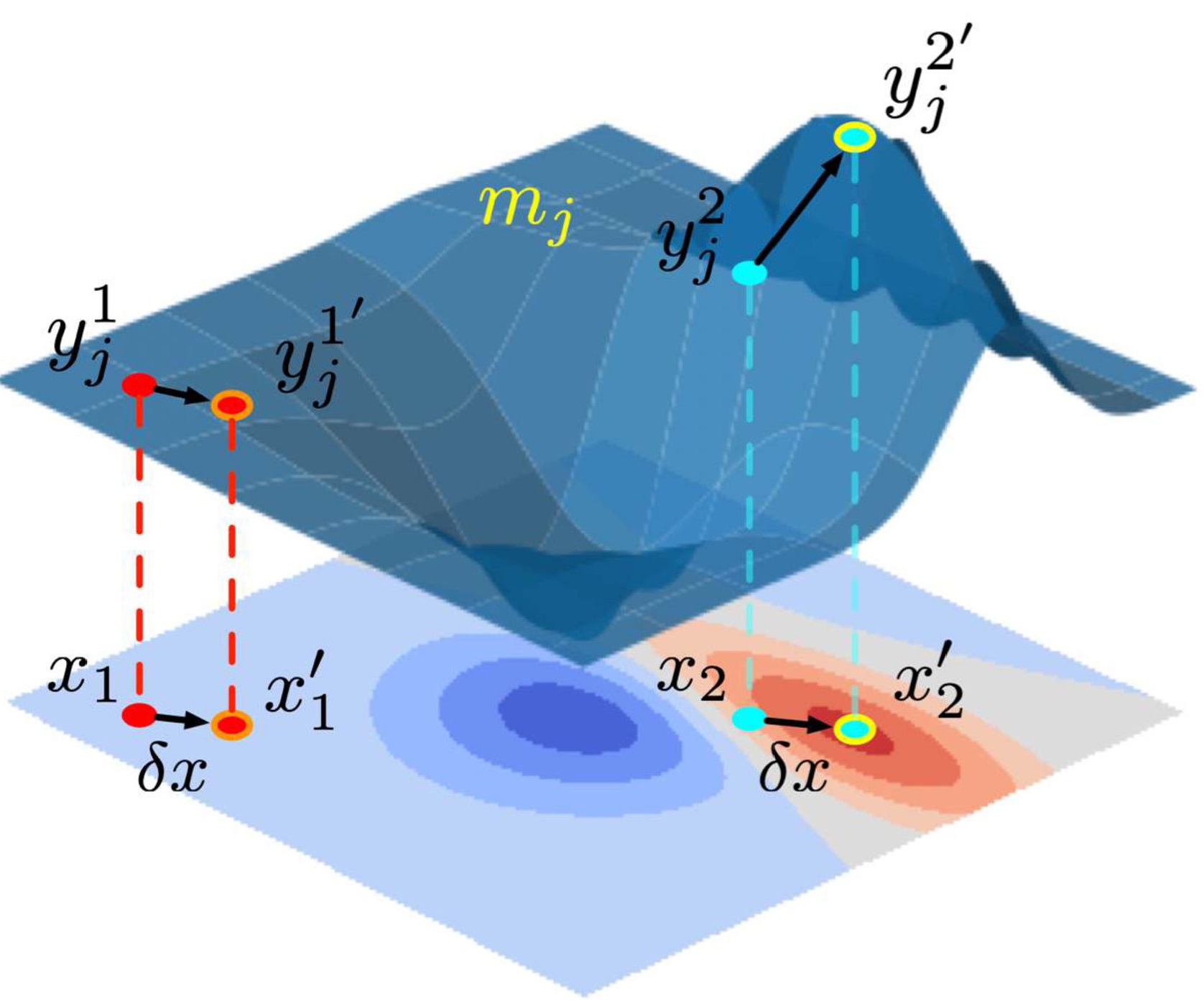
(a) 3D Hypersurface

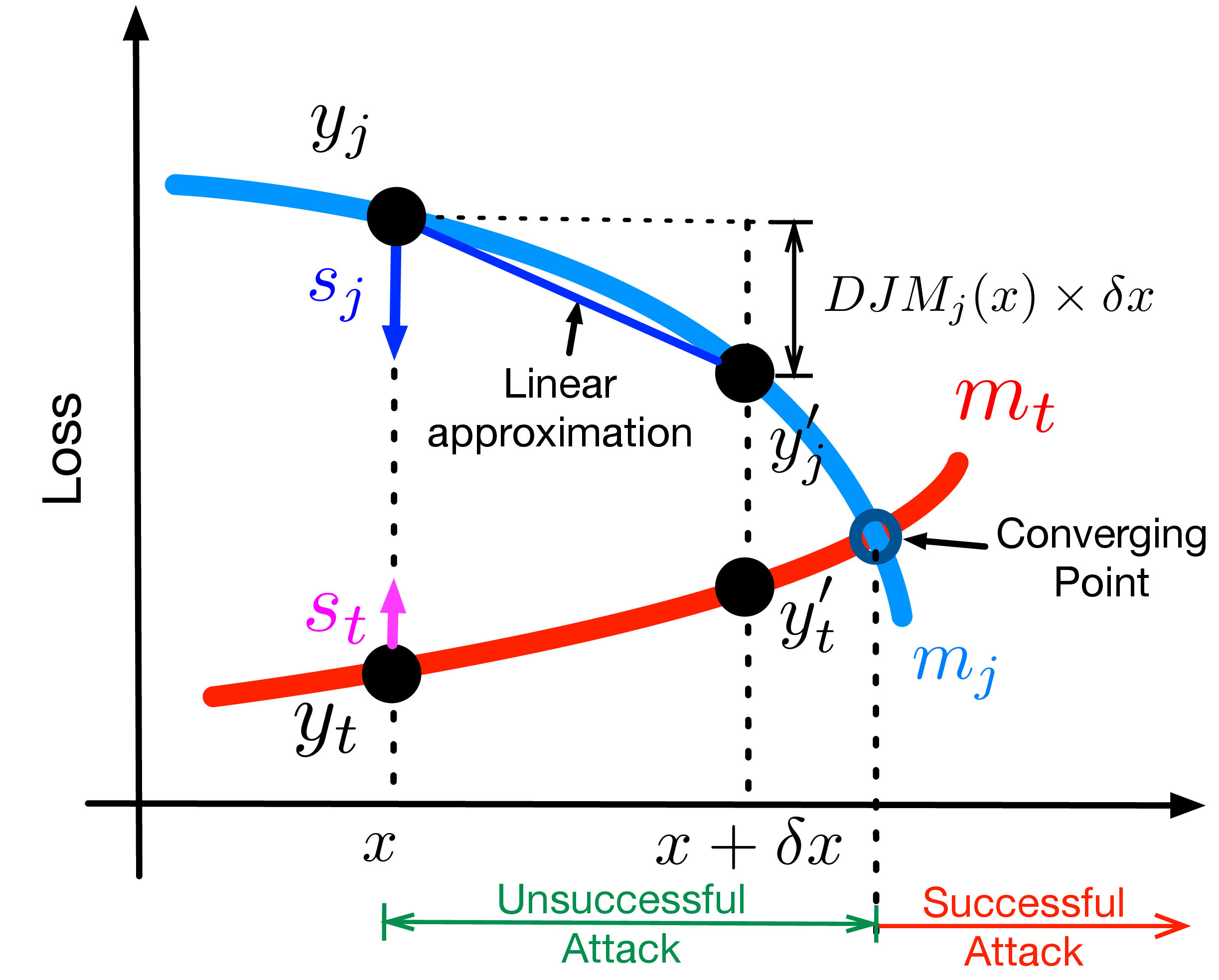
(b) Intuitions behind ACTS

Figure 1. (a) An example of 3D hypersurface, (b) intuition behind our ACTS.

3.1. Adversarial Converging Time Score

Adversarial Attacks in Image Classification Given an $M$ dimensional input $x\in\mathbf{R}^{M}$ and a K-class classification loss function $D:\mathbf{R}^{M}\rightarrow\mathbf{R}^{K}$, the predicted class label $t$ of the input $x$ is defined as:

(1) $$t=C(x)=\underset{j}{\mathrm{argmin}}\{y_{j}\mid y_{j}\in\mathbf{R}^{1}\},$$

where $y_{j}$ is the $j$th element of the $K$-dimensional output of $D(x)$. From geometrical point of view, $y_{j}$ can be regarded as a point on a $M+1$ dimensional hypersurface $m_{j}$ (See Fig. 1 (a)).

Since DNN-based classifiers are typically non-linear systems, which is true for all state-of-the-art DNN models. In this case, the hypersurfaces $m$ defined by $D$ are also non-linear systems. Thus, local areas around different points on a hypersurface $m_{j}$ have different curvatures, which results in that different inputs would have different sensitivity to the same added noise $\delta{x}$. As shown in Fig. 1 (a), the changes on a hypersurface $m_{j}$ driven by the same $\delta{x}$ are significantly different in terms of magnitude. Inspired by this insight, we propose a novel Adversarial Converging Time Score (ACTS) as an instance-specific adversarial robustness metric. The key to the proposed ACTS is that the sensitivity is mapped to the “time” required to reach the converging curve (i.e., decision boundary) where a clean sample is converted to an adversarial sample. We first introduce the proposed ACTS in detail. Then, we provide a toy-example to validate the proposed approach.

Adversarial Converging Time Score (ACTS) To easily convey the intuitive idea of the proposed ACTS, we use 1D input domain and 2D hypersurface (i.e., lines). Fig. 1 (b) shows our idea intuitively. As we can see, based on Eq. 1, the original input $x$ is classified as $t$th class since $y_{t}$ is in a lower position than $y_{j}$ in the loss domain. Although adding a noise $\delta{x}$ to $x$ results in two new positions $y_{t}^{\prime}$ and $y_{j}^{\prime}$, the predicted label of $x+\delta{x}$ is not changed (still $t$). If $x+\delta{x}$ passes the converging point, the predicted label of $x+\delta{x}$ changes to $j$. From this point of view, the robustness of an input can be reflected by the magnitude of the added $\delta{x}$ for reaching the converging point. For a DNN-based classifier, the collection of converging points forms the decision boundary. However, such decision boundary is extremely hard to be estimated, especially in a high-dimensional space. Instead, we can look at the converging point from the perspective of loss domain, where the distance between $y_{j}^{\prime}$ and $y_{t}^{\prime}$ is $0$. In other words, the robustness of an input can be reflected by the time used to cover the distance $y_{j}-y_{t}$, i.e., the less time it requires, the less robust it is. Compared to the decision boundary estimation, estimating the distance $y_{j}-y_{t}$ is much easier. Hence, we propose the ACTS to estimate such time, which takes the following form:

(2) $$ACTS :=\underset{j}{\mathrm{argmin}}(f(\frac{y_{j}-y_{t}}{s_{t}-s_{j}}))\quad j\in 1\ldots K,j\neq t,$$

$$f(x) =\begin{cases}C,&x\leq 0\\ x,&x>0\end{cases}$$

where $s_{j}$ and $s_{t}$ are the moving speeds in the loss domain, which are driven by the added noise $\delta{x}$. However, the minus sign in the denominator may be a bit tricky. An ideal misclassification attack should increase the target error value, results in a positive $s_{t}$, and it should also decrease the error value of the potential misclassified class, which gives a negative $s_{j}$ (as shown in Fig. 1(b)). Hence, the value of $s_{t}-s_{j}$ should always be positive. However, the $s_{t}-s_{j}$ could be a negative value in the following situations: (a) $s_{t}$ decreases and $s_{j}$ increases; (b) both of $s_{t}$ and $s_{j}$ decrease, but $s_{t}$ decreases faster; (c) both of $s_{t}$ and $s_{j}$ increase, but $s_{j}$ increases faster. If any of the above cases happen to an input, it means it is impossible to deliver a successful attack, and hence the ACTS of the specific input is a maximum score $C$. The $f(x)$ used in the Eq. (2) is for this purpose. Since ACTS represents the time to cover the distance $y_{j}-y_{t}$ with a speed $s_{t}-s_{j}$, an input with a smaller ACTS is more vulnerable to an adversarial attack, and vice-versa.

The key to the proposed ACTS is to estimate the moving speed. However, a local neighborhood on an output hypersurface is non-linear. It is very challenging to estimate the moving speed directly. To this end, we propose a novel $DJM$ based scheme to estimate the required moving speed, which takes the non-linearity nature of an output hypersurface into account.

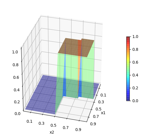
(a) Model output

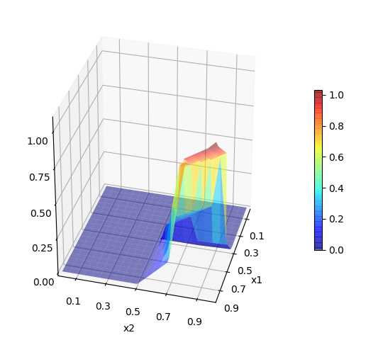
(b) ACTS distribution

Figure 2. (a) the output of the toy example AND gate model, (b) the ACTS distribution of the toy example AND gate model for all input samples where $x_{1}\wedge x_{2}=1$.

Data Jacobian Matrix Given an input $x$, the Data Jacobian Matrix (DJM) of $D$ is defined as:

(3) $$DJM(x)=\frac{\partial{D(x)}}{\partial{x}}=\begin{bmatrix}\frac{\partial{D_{j}(x)}}{\partial{x_{i}}}\end{bmatrix}_{j\in 1\ldots K,i\in 1\ldots M}$$

On a hypersurface $m_{j}$, the $DJM_{j}(x)$ (i.e., $j$th row of $DJM(x)$) defines the best linear approximation of $D$ for points close to point $x$ (Wikipedia, 2018). Therefore, with $DJM(x)$, a small change $\delta{x}$ in the input domain of $D$ can be linearly mapped to the change on the hypersurfaces $m_{j}$. Mathematically, it can be described as:

(4) $$D(x+\delta{x})=D(x)+DJM(x)\times\delta{x}+\delta{e},$$

where $\delta{e}\in R^{K}$ is the approximation error. Essentially, the $DJM(x)$ is very similar to the gradient backpropagated through a DNN during a training process. The only difference is $DJM(x)$ differentiates with respect to the input $x$ rather than network parameters.

One-step attack Based on the Eq. (4), with an input $x$ and an added noise $\delta{x}$, the original point $y_{j}(a.k.a.,D_{j}(x))$ is shifted to the point $y_{j}^{\prime}$ on the hypersurface $m_{j}$, and the approximated shifted position of $y_{j}^{\prime}$ can be estimated as (shown in Fig. 1 (b)):

(5) $$y_{j}^{\prime}\approx D_{j}(x)+DJM_{j}(x)\times\delta{x},$$

where $DJM_{j}(x)$ is the $j$th row of the $DJM(x)$. For one-step attack (e.g., FGSM), $\delta{x}$ can be regarded as a vector $\vec{d}$. The direction of $\vec{d}$ is fixed and only the length of $\vec{d}$ varies for delivering a successful attack. Therefore, the moving speed $s_{j}$ from point $y_{j}$ to $y_{j}^{\prime}$ on the surface $m_{j}$ driven by the shift $\delta{x}$ in the input domain can be estimated as:

(6) $$s_{j}=\frac{y_{j}^{\prime}-y_{j}}{\|\delta{x}\|}\approx\frac{DJM_{j}(X)\times\delta{x}}{\|\delta{x}\|}\quad j\in 1\ldots K.$$

It is worth to mention that the $DJM$ is an linear approximation for a small $\delta{x}$. The approximation accuracy decreases while $\delta{x}$ increases.

Multi-step attack In a multi-step attack (e.g., BIM), each step changes the $\vec{d}$ (i.e., $\delta{x}$) in terms of both direction and length. Compared to one-step attacks, the different directions reveal more curvatures of a local neighborhood, and it increases the probability of discovering a more optimal moving speed to reduce the “time” (i.e., added noise) for converting a clean sample to an adversarial one. That is also the reason that multi-step attacks are more effective than one-step attacks. However, the dynamics introduced by multi-step attacks is also troublesome to estimate the desired moving speed. To deal with it, we propose an average moving speed from $y_{j}$ to $y_{j}^{\prime}$ based on all explored directions as follow:

(7) $$s_{j}\approx\frac{1}{N}\sum_{q}^{N}\frac{DJM_{j}(x)\times\delta{x_{q}}}{\|\delta{x_{q}}\|}\quad j\in 1\ldots K,$$

where $N$ is the total steps used in the multi-step attack, and $\delta{x_{q}}$ is the added noise in the $q$th step. Even though the estimated average speed has limited accuracy, our experiments show the effectiveness of the proposed average speed.

3.2. Toy Example

We design a toy experiment to validate the proposed ACTS, where a simple two-layer feed-forward network was trained to proximate a AND gate. The testing accuracy of the trained model was 99.7%. Mathematically, we define the AND gate as:

$$x_{1}\wedge x_{2} =1,\quad x_{1}\geq 0.5\text{ and }x_{2}\geq 0.5$$

$$x_{1}\wedge x_{2} =0,\quad\text{ otherwise}$$

where $x_{i}\in[0,1.0]$. Based on this definition, as shown in Fig. 2 (a), [0.5, 1.0] is the decision boundaries on both $x_{1}$ and $x_{2}$ axes, where lower ACTSs are expected. We use FGSM method, with $\epsilon=0.1$, to generate adversarial samples only for the clear sample pairs of $x_{1}\wedge x_{2}=1$. For the rest pairs, ACTSs are set to 0. As shown in Fig. 2 (b), the input pairs closer to the decision boundary have lower ACTSs. Also, we observe an increasing trend in the ACTSs as the input values move further away from the boundary. The maximum ACTS is observed at point $(x_{1},x_{2})=(1.0,1.0)$. These observations illustrate the proposed ACTSs is able to reflect the robustness under the FGSM attack.

4. Experiments

In this section, we first validate the effectiveness and generalization capacity of the proposed ACTS metric against different state-of-the-art DNN models and adversarial attack approaches on the ImageNet (Deng et al., 2009) dataset in Section 4.2. We then compare the proposed ACTS with CLEVER (Weng et al., 2018b) (the only method that can be adapted to deep models and large-scale ImageNet dataset), to show that our method provides a more effective and practical robustness metric in different adversarial settings in Section 4.3.

4.1. Experimental Setting

Evaluation dataset and methods To evaluate the effectiveness of proposed method on large-scale datasets, we choose the ImageNet Large Scale Visual Recognition Challenge (ILSVR) 2012 dataset, which has 1.2 million training and 50,000 validation images. We evaluate our method on three representative state-of-the-art deep networks with pre-trained models provided by PyTorch (Paszke et al., 2017), i.e., the InceptionV3 (Szegedy et al., 2016), ResNet50 (He et al., 2016) and VGG16 (Simonyan and Zisserman, 2014), as these deep networks have their own network architectures. To evaluate the robustness of our method against different attacks, we consider three different state-of-the-art white-box attack approaches, i.e.,  (FGSM (Goodfellow et al., 2014), BIM (Kurakin et al., 2016), and PGD (Madry et al., 2017)).

Implementation details We have implemented our ACTS using the PyTorch framework, and all attack methods using the adversarial robustness PyTorch library: Torchattacks (Paszke et al., 2019). A GPU-Server with an Intel E5-2650 v4 2.20GHz CPU (with 32GB RAM) and one NVIDIA Tesla V100 GPU (with 24GB memory) is used in our experiments. For preprocessing, we normalize the data using mean and standard deviation. The images are loaded in the range of $[0,1]$ and then normalized using a $mean=[0.485,0.456,0.406]$ and $std=[0.229,0.224,0.225]$ (Paszke et al., 2017). To control the noise levels in order not to bring any noticeable perceptual differences and show the consistent performance of the proposed ACTS, we add the noise of three different levels: $\epsilon=\{0.00039~{}(0.1/255)$, $0.00078~{}(0.2/255)$, $0.00117~{}(0.3/255)\}$ to the FGSM (Goodfellow et al., 2014), BIM (Kurakin et al., 2016) and PGD (Madry et al., 2017), respectively. We use N1, N2 and N3 to represent these three different noise levels, respectively. We use three steps and set the step size = $\epsilon/2$ to both BIM (Kurakin et al., 2016) and PGD (Madry et al., 2017). We use the untargeted attack setting in all attacks. For each image, we evaluate its top-10 class (i.e., the class with the top-10 maximum probabilities except for the true class, which is usually the easiest target to attack) (Weng et al., 2018b) in $DJM$.

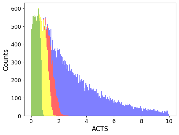
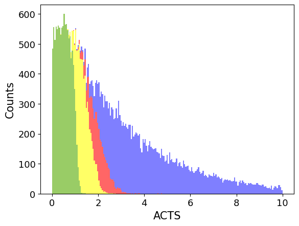
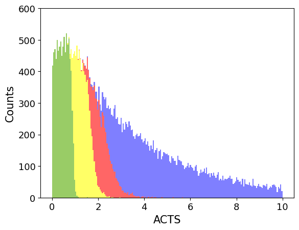
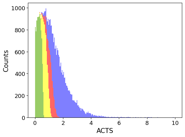
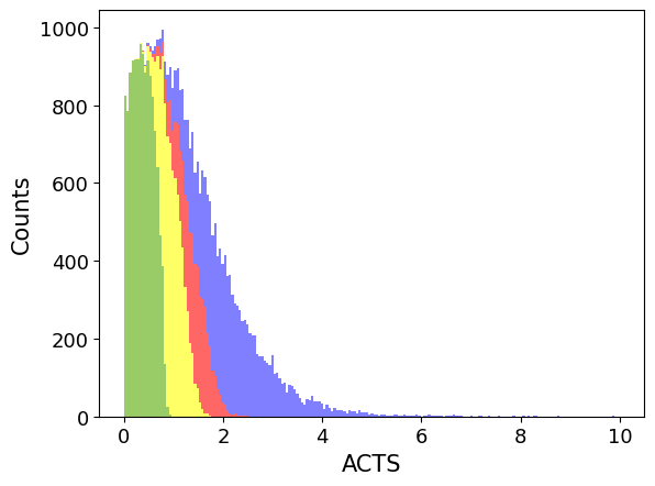
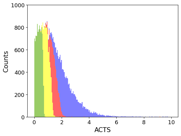
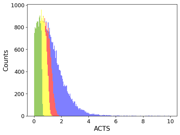
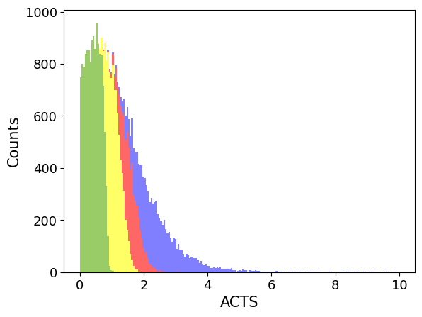
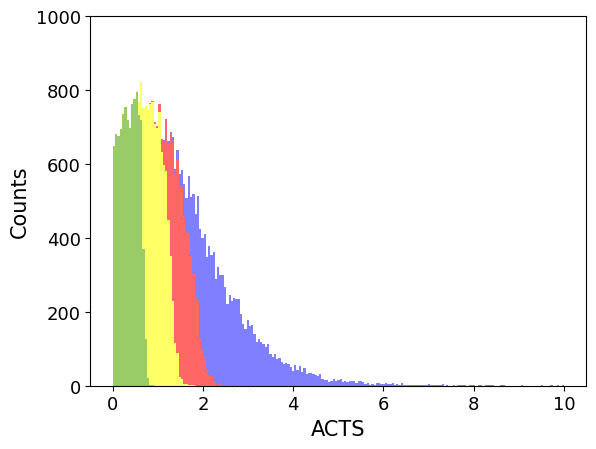
(a) InceptionV3-FGSM (b) InceptionV3-BIM (c) InceptionV3-PGD (d) ResNet50-FGSM (e) ResNet50-BIM (f) ResNet50-PGD (g) VGG16-FGSM (h) VGG16-BIM (i) VGG16-PGD   (Green): $\epsilon=\{0.1,0.00039\}$   (Yellow): $\epsilon=\{0.2,0.00078\}$   (Red): $\epsilon=\{0.3,0.00117\}$   (Blue): $\epsilon=\{0.05,0.00020\}$ Figure 3. Noise Effectiveness charts for different models under different attacks. Area under the blue color denotes ACTS scores for the correctly classified samples on ImageNet validation dataset . Green, yellow, red colors denoted the ACTS scores of the samples that were successfully attacked. Each color denotes the noise level added to the dataset with respect to the corresponding attack.

4.2. ACTS Validation Results

This section evaluates the effectiveness and generalization properties of our proposed ACTS method in various adversarial environments.

Table 1. Clean and Adversarial accuracy in different adversarial environments.

Attack	Model	Clean	Adversarial  Accuracy
			N1	N2	N3
FGSM	InceptionV3	77.21%	61.16%	50.03%	43.05%
	ResNet50	76.13%	57.45%	43.94%	34.77%
	VGG16	71.59%	52.35%	37.73%	27.71%
BIM	InceptionV3	77.21%	55.10%	43.05%	36.68%
	ResNet50	76.13%	50.08%	34.77%	25.47%
	VGG16	71.59%	44.38%	27.71%	18.46%
PGD	InceptionV3	77.21%	60.20%	45.86%	36.31%
	ResNet50	76.13%	56.13%	39.15%	26.56%
	VGG16	71.59%	51.77%	34.48%	22.28%

Evaluating the effectiveness of ACTS To be an effective adversarial robustness metric, the proposed ACTS should faithfully reflect that the samples with lower ACTS scores are more prone to be attacked successfully than those with higher scores. To validate such property of the ACTS, we design the following experiments. First, we apply these three DNN models on the ImageNet validation dataset and selected those correctly classified images. Secondly, we estimate the ACTS scores for all the selected images and apply the three chosen attack methods to them. It can be seen from Table 1 that, the adversarial accuracy is gradually decreased to a moderate extent with increased levels of noise. Third, in order to show the consistent performance of the proposed ACTS, we increase the noise level to N1, N2 and N3 and record the ACTS scores for those who are successfully attacked. Fig. 3 shows the histograms of the three chosen DNN models under different attacks, respectively. The blue color indicates the ACTS scores of the images that are correctly classified on ImageNet validation dataset under the initial noise $\epsilon$ = 0.0002, and the other three colors indicate the ones that are attacked successfully with noise level N1, N2 and N3. For all the models and attacks, the green, yellow and red regions are always on the very left side of the respective charts. This shows the inputs with lower ACTS scores are easier to be attacked successfully. We can also see that with increased noise levels, images with relatively lower ACTS scores would be attacked successfully first (from green to red). In addition, Fig. 3 and Table 1 show that these aforementioned observations are consistent in different adversarial environments (i.e., different DNN architectures and different attacks). Based on the distribution of the obtained ACTS, we are able to gain a relatively precise intuition about DNNs’ performance under different attack methods. For example, based on the each row figures of Fig. 3, it is obvious that ACTS histograms of green, yellow, red colors become much wider range than previous, which indicate BIM and PGD are more powerful attack methods when compared to FGSM attack method. This observations can be confirmed by the corresponding adversarial accuracy rates shown in Table 1.

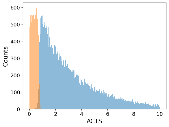
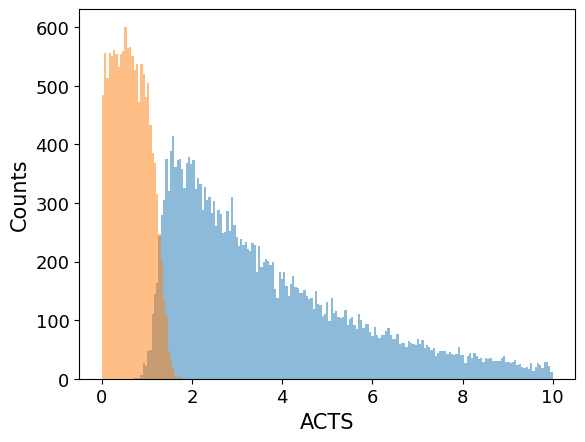
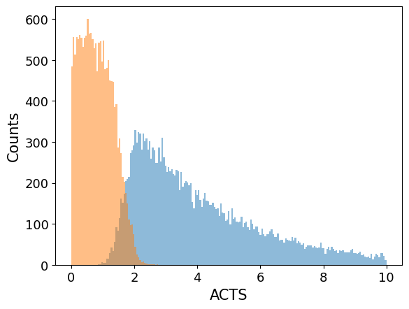
(a) InceptionV3-FGSM-N1	(b) InceptionV3-FGSM-N2	(c) InceptionV3-FGSM-N3
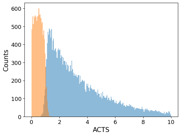
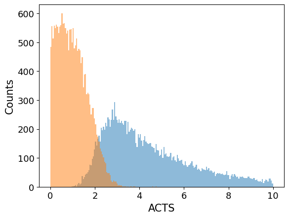
(d) InceptionV3-BIM-N1	(e) InceptionV3-BIM-N2	(f) InceptionV3-BIM-N3
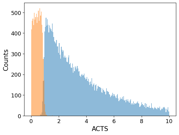
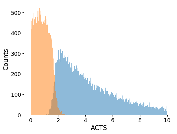
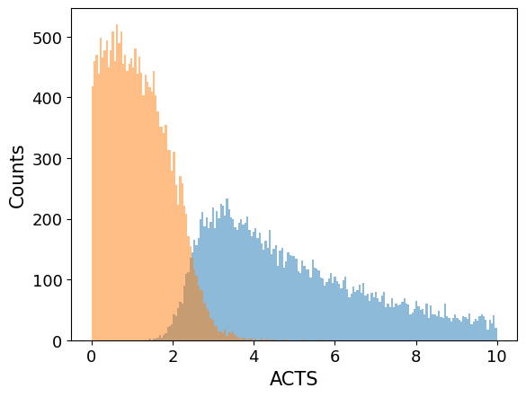
(g) InceptionV3-PGD-N1	(h) InceptionV3-PGD-N2	(i) InceptionV3-PGD-N3

Figure 4. ACTS scores histograms of InceptionV3 in different experimental configurations. In each histogram, the orange color indicates the samples that are attacked successfully, and the light blue color indicates the ones that are attacked unsuccessfully.

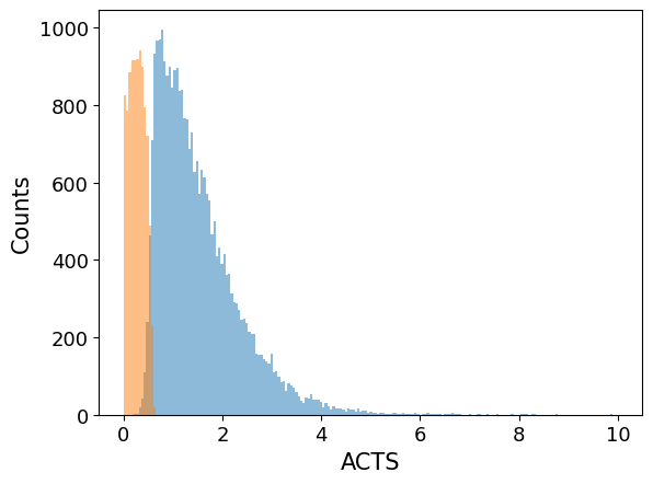
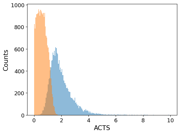
(a) ResNet50-FGSM-N1	(b) ResNet50-FGSM-N2	(c) ResNet50-FGSM-N3
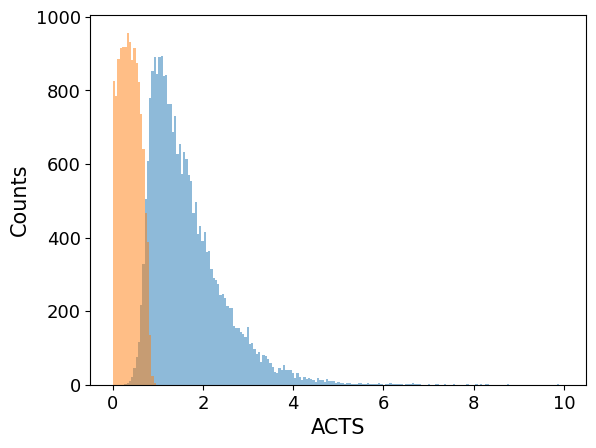
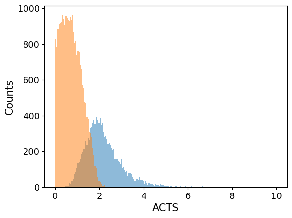
(d) ResNet50-BIM-N1	(e) ResNet50-BIM-N2	(f) ResNet50-BIM-N3
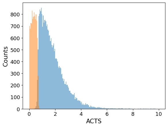
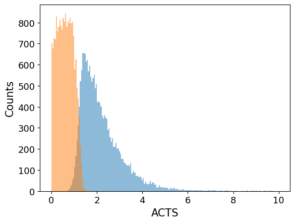
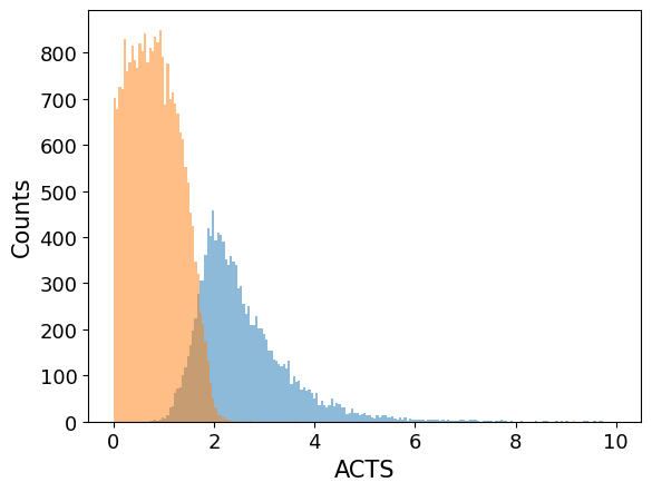
(g) ResNet50-PGD-N1	(h) ResNet50-PGD-N2	(i) ResNet50-PGD-N3

Figure 5. ACTS scores histograms of ResNet50 in different experimental configurations. In each histogram, the orange color indicates the samples that are attacked successfully, and the light blue color indicates the ones that are attacked unsuccessfully.

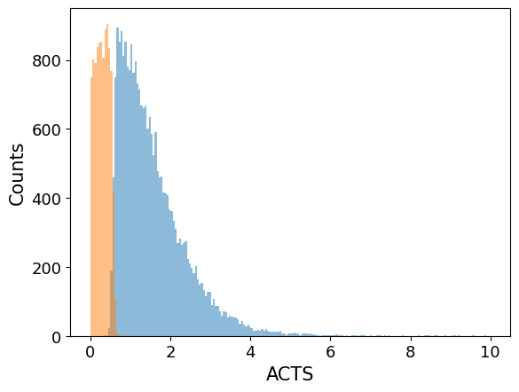
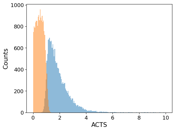
(a) VGG16-FGSM-N1	(b) VGG16-FGSM-N2	(c) VGG16-FGSM-N3
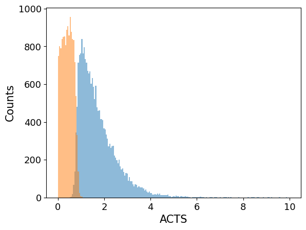
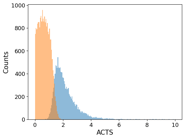
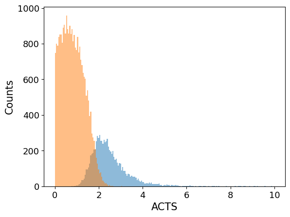
(d) VGG16-BIM-N1	(e) VGG16-BIM-N2	(f) VGG16-BIM-N3
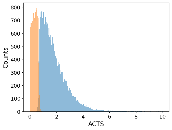
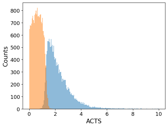
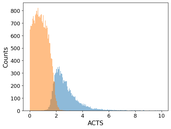
(g) VGG16-PGD-N1	(h) VGG16-PGD-N2	(i) VGG16-PGD-N3

Figure 6. ACTS scores histograms of VGG16 in different experimental configurations. In each histogram, the orange color indicates the samples that are attacked successfully, and the light blue color indicates the ones that are attacked unsuccessfully.

Table 2. ACTS Overlap% values in different adversarial environments.

Attack	Model	Overlap% N1	Overlap% N2	Overlap% N3
FGSM	InceptionV3	1.46%	3.54%	4.71%
	ResNet50	2.95%	6.42%	9.14%
	VGG16	2.14%	4.29%	5.71%
BIM	InceptionV3	2.53%	4.71%	6.26%
	ResNet50	4.89%	9.13%	10.89%
	VGG16	3.02%	5.71%	6.47%
PGD	InceptionV3	1.33%	3.26%	4.85%
	ResNet50	1.72%	4.70%	6.62%
	VGG16	1.87%	3.73%	4.89%

Table 3. Numbers of images in ImageNet for different architectures found in different ‘attack flip’ experimental configurations. ‘1’ means attack flip between different noise level N1 and N2. ‘2’ means attack flip between different noise level N1 and N3. ‘3’ means attack flip between different noise level N2 and N3.

Attack type	FGSM			BIM			PGD
Attack Flip	1	2	3	1	2	3	1	2	3
InceptionV3	0	0	1	1	10	10	0	0	2
ResNet50	0	1	1	0	3	5	1	0	3
VGG16	0	0	0	0	3	4	2	3	8

In addition to the qualitative results in Fig. 3, we also present the quantitative results to show the effectiveness of ACTS. Fig. 4, Fig. 5 and Fig. 6 show the detailed histogram results in different adversarial environments. The orange color indicates the samples that are attacked successfully, and the light blue color indicates the ones that are attacked unsuccessfully. Only an ideal robustness metric could separate the two groups without any overlap, and existing approaches may have different overlap regions between the two groups. Hence, the size of overlap regions can be leveraged as an indicator to show the effectiveness of a robustness metric. For each histogram, we calculate the overlap percentage by $S_{o}/S_{a}$, where $S_{o}$ is the size (i.e., count) of an overlap area, and $S_{a}$ is the total area of a histogram. Hence, for Overlap%, the lower its values, the better the evaluating results are. All results are shown in Table 2. As we can see, almost all Overlap% values are below 10%. In terms of DNN architecture, ACTS shows better performance on InceptionV3 and VGG16. We guess the reason is the local areas on output hypersurfaces of InceptionV3 and VGG16 around the output points of all tested images are flatter (i.e., the radius of curvature is small) than ResNet50. In this case, the $DJM$ provides a more accurate linear approximation. It is worth to mention that the overlap area is getting larger when $\epsilon$ increases in different adversarial environments. It confirms with the limitation of the DJM that the linear approximation accuracy decreases while $\delta{x}$ increases. In the process of statistics, we found an interesting phenomenon called the attack flip: the image with a successful attack at a lower noise level may fail at a higher noise level. The result is shown in Table 3. Attack flip is a good explanation for why there are very small ACTS scores in the overlap at a higher noise level. In other words, some small ACTS scores are counted as orange histogram at a lower noise level and then counted as blue histogram at a higher noise level. This flip will result in small ACTS scores in the overlap at a higher noise level. Besides, another reason is that the limitation of the DJM. The linear approximation accuracy of the DJM decreases while $\delta{x}$ increases which will lead to the error. Attack flip also suggests that the lower bound may not always make sense.

Evaluating the Generalization of ACTS In Fig. 3, the histogram of each row represent the results of the same model under different attack, and each column represent the results of different models under the same attack method. From the results, we can see that ACTS has a good generalization ability across different attack methods and models.

Correlations to CLEVER We are interested in whether our ACTS align with the CLEVER. To this end, we compute the average score of all the tested images as the CLEVER’s reported robustness number. The higher the CLEVER score, the more robust the model is. We also calculate the average ACTS score of all the tested images to represent the robustness of the network. From the results shown in Table 4, we get the same ranking correlation to CLEVER. It also demonstrates that models with higher ACTS scores are more robust. The results we obtained are basically consistent with the results in Table (3) (b) of CLEVER (The column of Top-2 Target) (Weng et al., 2018b). Besides, we conclude that VGG16 model with highest scores are more robust than other on test image set. This conclusion can also be found in (Su et al., 2018). It is worth to mention that the score distribution may change dramatically on different test image sets.

Table 4. Using CLEVER method and ACTS method to measure the ranking correlation of the robustness of different models.

Model	CLEVER	ACTS
VGG16	0.370	4.459
InceptionV3	0.215	3.047
ResNet50	0.126	2.558

Determining k To investigate the impact of the top-k class in $DJM$, for each image, we evaluate its top-k class ACTS scores in Table 5. From the results, we can see that with the increase of k, the value of Overlap% changes very slightly. Considering the balance between computational consumption and ACTSs’ performance, it is reasonable to set the k to 10.

Table 5. Top-k class ACTS Overlap% values in different environments.

Attack	Model	Metric	Overlap% N1	Overlap% N2	Overlap% N3
FGSM	InceptionV3	ACTS-10	1.56%	2.08%	5.2%
		ACTS-20	1.56%	2.08%	5.2%
		ACTS-50	1.56%	2.08%	5.2%
	ResNet50	ACTS-10	2.39%	7.98%	9.84%
		ACTS-20	2.39%	7.98%	9.71%
		ACTS-50	2.39%	7.98%	9.71%
	VGG16	ACTS-10	1.3%	3.46%	6.63%
		ACTS-20	1.3%	3.46%	6.77%
		ACTS-50	1.3%	3.46%	6.92%
BIM	InceptionV3	ACTS-10	1.43%	5.2%	6.37%
		ACTS-20	1.43%	5.2%	6.37%
		ACTS-50	1.43%	5.2%	6.37%
	ResNet50	ACTS-10	4.39%	9.84%	10.9%
		ACTS-20	4.26%	9.71%	11.17%
		ACTS-50	4.26%	9.71%	11.17%
	VGG16	ACTS-10	2.74%	3.63%	5.91%
		ACTS-20	2.74%	3.63%	5.91%
		ACTS-50	2.74%	3.63%	5.91%
PGD	InceptionV3	ACTS-10	0.91%	3.25%	4.81%
		ACTS-20	0.91%	3.25%	4.42%
		ACTS-50	0.91%	2.99%	4.68%
	ResNet50	ACTS-10	0.93%	5.32%	6.12%
		ACTS-20	0.93%	5.45%	6.52%
		ACTS-50	0.93%	5.19%	6.38%
	VGG16	ACTS-10	1.3%	3.03%	4.61%
		ACTS-20	1.44%	3.17%	4.61%
		ACTS-50	1.44%	3.17%	4.76%

4.3. Comparing With the State-of-the-art CLEVER

We compare our method with state-of-the-art method CLEVER in this section. CLEVER score is designed for estimating the lower bound on the minimal distortion required to craft an adversarial sample, and it used $L_{2}$ and $L_{\infty}$ norms for their validations. We follow the setting in (Weng et al., 2018b) to compute CLEVER $L_{2}$ and $L_{\infty}$ norms scores for 1,000 images out of the all 5,0000 ImageNet validation set, as CLEVER is more computational expensive. The same set of randomly selected 1,000 images from the ImageNet validation set is also used in our method. Instead of sampling a high-dimension-space ball, our method only requires normal backpropagations, which is significantly faster than CLEVER. Our experiment results in Table 6 confirm this.

Table 6. The average computation time of CLEVER and ACTS on different models for a single image in ImageNet. Blue and red fonts in the third column represent ACTS average computation time under one-step and multi-step attacks, respectively. The fourth column is the corresponding lifting multiple.

Model	Metric	Average Computation Time (second)	ACTS speed_up
InceptionV3	CLEVER	331.42	6628/2549
	ACTS	0.05/0.13
ResNet50	CLEVER	196.25	4906/2181
	ACTS	0.04/0.09
VGG16	CLEVER	286.85	5737/2207
	ACTS	0.05/0.13

For each image, we calculate its CLEVER and ACTS scores on an NVIDIA Tesla V100 graphics card, the average computation speed of our method is three orders of magnitude faster than CLEVER method on different models. We also use the Overlap% indicator to compare the effectiveness of different robustness metrics, inspired by the ROC curve, which visualizes all possible classification thresholds to quantify the performance of a classifier. Since ACTS and CLEVER only care about whether the distribution of image scores are consistent with successful/unsuccessful results in different adversarial environments, we can use the Overlap% indicator as “mis-classification rate”. In Table 7, we calculate $L_{2}$ CLEVER, $L_{\infty}$ CLEVER and ACTS Overlap% values respectively. From the results, we can see that the value range of the $L_{2}$ CLEVER and $L_{\infty}$ CLEVER Overlap% is almost in 10% ~ 20%, and the value range of the ACTS Overlap% is almost in 0% ~ 10%. CLEVER scores have almost more than twice larger Overlap% values on average for all testing configurations. Even though $L_{\infty}$ CLEVER scores give slightly less Overlap% values than the ones based on $L_{2}$ CLEVER scores, ACTS still outperform them in a significant margin with all testing configurations. These results indicate that ACTS is a more effective metric than CLEVER in different adversarial environments.

Table 7. Comparing ACTS with CLEVER Overlap% values in different adversarial environments.

Attack	Model	Metric	Overlap% N1	Overlap% N2	Overlap% N3
FGSM	InceptionV3	$L_{2}$ CLEVER	14.34%	15.36%	17.80%
		$L_{\infty}$ CLEVER	13.7%	15.88%	17.67%
		ACTS	1.56%	2.08%	5.2%
	ResNet50	$L_{2}$ CLEVER	17.11%	18.6%	19.14%
		$L_{\infty}$ CLEVER	13.61%	15.5%	17.25%
		ACTS	2.39%	7.98%	9.84%
	VGG16	$L_{2}$ CLEVER	10.43%	11.59%	13.48%
		$L_{\infty}$ CLEVER	8.99%	10.43%	12.75%
		ACTS	1.3%	3.46%	6.63%
BIM	InceptionV3	$L_{2}$ CLEVER	11.91%	12.16%	10.88%
		$L_{\infty}$ CLEVER	11.91%	11.65%	10.5%
		ACTS	1.43%	5.2%	6.37%
	ResNet50	$L_{2}$ CLEVER	16.44%	16.31%	14.42%
		$L_{\infty}$ CLEVER	13.34%	15.23%	13.34%
		ACTS	4.39%	9.84%	10.9%
	VGG16	$L_{2}$ CLEVER	10.72%	11.45%	14.2%
		$L_{\infty}$ CLEVER	9.13%	10.58%	13.19%
		ACTS	2.74%	3.63%	5.91%
PGD	InceptionV3	$L_{2}$ CLEVER	12.04%	11.4%	11.91%
		$L_{\infty}$ CLEVER	11.01%	11.27%	11.78%
		ACTS	0.91%	3.25%	4.81%
	ResNet50	$L_{2}$ CLEVER	14.15%	15.77%	14.82%
		$L_{\infty}$ CLEVER	12.13%	12.94%	12.8%
		ACTS	0.93%	5.32%	6.12%
	VGG16	$L_{2}$ CLEVER	7.54%	10.14%	13.77%
		$L_{\infty}$ CLEVER	7.68%	8.7%	12.17%
		ACTS	1.3%	3.03%	4.61%

5. Conclusion and Future work

In this work, we have proposed the Adversarial Converging Time Score (ACTS) as an instance-specific adversarial robustness metric. ACTS is inspired by the geometrical insight of the output hypersurfaces of a DNN classifier. We perform a comprehensive set of experiments to substantiate the effectiveness and generalization of our proposed metric. Compared to CLEVER, we prove that ACTS can provide a faster and more effective adversarial robustness prediction for different attacks across various DNN models. More importantly, ACTS solves the adversarial robustness problem from a geometrical point of view. We believe it provides a meaningful angle and insight into the adversarial robustness problem, which will help the future work in the same vein.

In the future, we will focus on improving DNN’s adversarial performance by leveraging the proposed ACTS. Another interesting direction to look into is extending the ACTS to make it work under black-box attack methods.

References

- (1)
- Akhtar and Mian (2018) Naveed Akhtar and Ajmal Mian. 2018. Threat of Adversarial Attacks on Deep Learning in Computer Vision: A Survey. IEEE Access 6 (2018), 14410–14430.
- Athalye et al. (2018a) Anish Athalye, Nicholas Carlini, and David Wagner. 2018a. Obfuscated Gradients Give a False Sense of Security: Circumventing Defenses to Adversarial Examples. In International Conference on Machine Learning.
- Athalye et al. (2018b) Anish Athalye, Logan Engstrom, Andrew Ilyas, and Kevin Kwok. 2018b. Synthesizing Robust Adversarial Examples. In International Conference on Machine Learning.
- Bastani et al. (2016) Osbert Bastani, Yani Ioannou, Leonidas Lampropoulos, Dimitrios Vytiniotis, Aditya Nori, and Antonio Criminisi. 2016. Measuring neural net robustness with constraints. In Advances in neural information processing systems.
- Bhagoji et al. (2017) Arjun Nitin Bhagoji, Daniel Cullina, and Prateek Mittal. 2017. Dimensionality Reduction as a Defense against Evasion Attacks on Machine Learning Classifiers. arXiv:1704.02654 (2017).
- Brendel et al. (2018) Wieland Brendel, Jonas Rauber, and Matthias Bethge. 2018. Decision-Based Adversarial Attacks: Reliable Attacks Against Black-Box Machine Learning Models. In International Conference on Learning Representations.
- Carlini and Wagner (2017) Nicholas Carlini and David Wagner. 2017. Towards evaluating the robustness of neural networks. In IEEE Symposium on Security and Privacy.
- Chen et al. (2017) Pin Yu Chen, Yash Sharma, Huan Zhang, Jinfeng Yi, and Cho Jui Hsieh. 2017. EAD: Elastic-Net Attacks to Deep Neural Networks via Adversarial Examples. In AAAI Conference on Artificial Intelligence.
- Chen et al. (2017) Pin-Yu Chen, Huan Zhang, Yash Sharma, Jinfeng Yi, and Cho-Jui Hsieh. 2017. ZOO: Zeroth Order Optimization Based Black-box Attacks to Deep Neural Networks without Training Substitute Models. In Proceedings of the 10th ACM Workshop on Artificial Intelligence and Security.
- Cheng et al. (2018) Minhao Cheng, Thong Le, Pin-Yu Chen, Jinfeng Yi, Huan Zhang, and Cho-Jui Hsieh. 2018. Query-Efficient Hard-label Black-box Attack: An Optimization-based Approach. In International Conference on Learning Representations.
- Deng et al. (2009) J. Deng, W. Dong, R. Socher, L.-J. Li, K. Li, and L. Fei-Fei. 2009. ImageNet: A Large-Scale Hierarchical Image Database. In Proceedings of the IEEE conference on computer vision and pattern recognition.
- Ding et al. (2022) Jianchuan Ding, Bo Dong, Felix Heide, Yufei Ding, Yunduo Zhou, Baocai Yin, and Xin Yang. 2022. Biologically Inspired Dynamic Thresholds for Spiking Neural Networks. In Advances in Neural Information Processing Systems.
- Dong et al. (2020) Yinpeng Dong, Qi-An Fu, Xiao Yang, Tianyu Pang, Hang Su, Zihao Xiao, and Jun Zhu. 2020. Benchmarking Adversarial Robustness on Image Classification. In IEEE Conference on Computer Vision and Pattern Recognition.
- Dong et al. (2018) Yinpeng Dong, Fangzhou Liao, Tianyu Pang, Hang Su, Jun Zhu, Xiaolin Hu, and Jianguo Li. 2018. Boosting Adversarial Attacks with Momentum. In 2018 IEEE Conference on Computer Vision and Pattern Recognition.
- Dong et al. (2019a) Yinpeng Dong, Tianyu Pang, Hang Su, and Jun Zhu. 2019a. Evading Defenses to Transferable Adversarial Examples by Translation-Invariant Attacks. In 2019 IEEE Conference on Computer Vision and Pattern Recognition.
- Dong et al. (2019b) Yinpeng Dong, Hang Su, Baoyuan Wu, Zhifeng Li, Wei Liu, Tong Zhang, and Jun Zhu. 2019b. Efficient Decision-Based Black-Box Adversarial Attacks on Face Recognition. In 2019 IEEE Conference on Computer Vision and Pattern Recognition.
- Engstrom et al. (2017) Logan Engstrom, Brandon Tran, Dimitris Tsipras, Ludwig Schmidt, and Aleksander Madry. 2017. A Rotation and a Translation Suffice: Fooling CNNs with Simple Transformations. arXiv:1712.02779 (2017).
- Ferrari et al. (2022) Claudio Ferrari, Federico Becattini, Leonardo Galteri, and Alberto Del Bimbo. 2022. (Compress and Restore)N: A Robust Defense Against Adversarial Attacks on Image Classification. ACM TOMM (2022).
- Gehr et al. (2018) Timon Gehr, Matthew Mirman, Dana Drachsler-Cohen, Petar Tsankov, Swarat Chaudhuri, and Martin Vechev. 2018. AI2: Safety and Robustness Certification of Neural Networks with Abstract Interpretation. In IEEE Symposium on Security and Privacy.
- Ghosh et al. (2019) Partha Ghosh, Arpan Losalka, and Michael J Black. 2019. Resisting Adversarial Attacks using Gaussian Mixture Variational Autoencoders. In AAAI Conference on Artificial Intelligence.
- Goodfellow et al. (2014) Ian J Goodfellow, Jonathon Shlens, and Christian Szegedy. 2014. Explaining and harnessing adversarial examples. arXiv:1412.6572 (2014).
- He et al. (2016) Kaiming He, Xiangyu Zhang, Shaoqing Ren, and Jian Sun. 2016. Deep residual learning for image recognition. In Proceedings of the IEEE conference on computer vision and pattern recognition.
- Ilyas et al. (2018) Andrew Ilyas, Logan Engstrom, Anish Athalye, and Jessy Lin. 2018. Black-box Adversarial Attacks with Limited Queries and Information.. In International Conference on Machine Learning.
- Kannan et al. (2018) Harini Kannan, Alexey Kurakin, and Ian J. Goodfellow. 2018. Adversarial Logit Pairing. arXiv:1803.06373 (2018).
- Katz et al. (2017) Guy Katz, Clark W. Barrett, David L. Dill, Kyle Julian, and Mykel J. Kochenderfer. 2017. Reluplex: An Efficient SMT Solver for Verifying Deep Neural Networks. In International Conference on Computer Aided Verification.
- Kurakin et al. (2016) Alexey Kurakin, Ian Goodfellow, and Samy Bengio. 2016. Adversarial examples in the physical world. arXiv:1607.02533 (2016).
- Kurakin et al. (2018) Alexey Kurakin, Ian J. Goodfellow, Samy Bengio, Yinpeng Dong, Fangzhou Liao, Ming Liang, Tianyu Pang, Jun Zhu, Xiaolin Hu, Cihang Xie, Jianyu Wang, Zhishuai Zhang, Zhou Ren, Alan L. Yuille, Sangxia Huang, Yao Zhao, Yuzhe Zhao, Zhonglin Han, Junjiajia Long, Yerkebulan Berdibekov, Takuya Akiba, Seiya Tokui, and Motoki Abe. 2018. Adversarial Attacks and Defences Competition. arXiv:1804.00097 (2018).
- Li et al. (2020) H. Li, G. Li, and Y. Yu. 2020. ROSA: Robust Salient Object Detection against Adversarial Attacks. IEEE Transactions on Cybernetics (2020).
- Li et al. (2021) Jiguo Li, Xinfeng Zhang, Jizheng Xu, Siwei Ma, and Wen Gao. 2021. Learning to Fool the Speaker Recognition. ACM TOMM (2021).
- Li et al. (2019) Yandong Li, Lijun Li, Liqiang Wang, Tong Zhang, and Boqing Gong. 2019. NATTACK: Learning the Distributions of Adversarial Examples for an Improved Black-Box Attack on Deep Neural Networks. In International Conference on Machine Learning.
- Liang et al. (2017) Bin Liang, Hongcheng Li, Miaoqiang Su, Xirong Li, Wenchang Shi, and Xiaofeng Wang. 2017. Detecting Adversarial Examples in Deep Networks with Adaptive Noise Reduction. arXiv:1705.08378 (2017).
- Liu et al. (2018a) Xuanqing Liu, Minhao Cheng, Huan Zhang, and Cho-Jui Hsieh. 2018a. Towards Robust Neural Networks via Random Self-ensemble. In Proceedings of the European Conference on Computer Vision.
- Liu et al. (2018b) Xuanqing Liu, Yao Li, Chongruo Wu, and Cho-Jui Hsieh. 2018b. Adv-BNN: Improved Adversarial Defense through Robust Bayesian Neural Network. In International Conference on Learning Representations.
- Madry et al. (2017) Aleksander Madry, Aleksandar Makelov, Ludwig Schmidt, Dimitris Tsipras, and Adrian Vladu. 2017. Towards deep learning models resistant to adversarial attacks. arXiv:1706.06083 (2017).
- Moosavi-Dezfooli et al. (2018) Seyed-Mohsen Moosavi-Dezfooli, Alhussein Fawzi, Omar Fawzi, Pascal Frossard, and Stefano Soatto. 2018. Robustness of Classifiers to Universal Perturbations: A Geometric Perspective. In International Conference on Learning Representations.
- Moosavi-Dezfooli et al. (2016) Seyed-Mohsen Moosavi-Dezfooli, Alhussein Fawzi, and Pascal Frossard. 2016. DeepFool: A Simple and Accurate Method to Fool Deep Neural Networks. In IEEE Conference on Computer Vision and Pattern Recognition.
- Pang et al. (2019) Tianyu Pang, Kun Xu, Chao Du, Ning Chen, and Jun Zhu. 2019. Improving Adversarial Robustness via Promoting Ensemble Diversity. In International Conference on Machine Learning.
- Papernot and McDaniel (2017) Nicolas Papernot and Patrick McDaniel. 2017. Extending Defensive Distillation. arXiv:1705.05264 (2017).
- Papernot et al. (2017) Nicolas Papernot, Patrick McDaniel, Ian Goodfellow, Somesh Jha, Z Berkay Celik, and Ananthram Swami. 2017. Practical black-box attacks against machine learning. In Proceedings of the ACM on Asia Conference on Computer and Communications Security.
- Papernot et al. (2016a) Nicolas Papernot, Patrick McDaniel, Somesh Jha, Matt Fredrikson, Z Berkay Celik, and Ananthram Swami. 2016a. The limitations of deep learning in adversarial settings. In IEEE Symposium on Security and Privacy.
- Papernot et al. (2016b) Nicolas Papernot, Patrick McDaniel, Xi Wu, Somesh Jha, and Ananthram Swami. 2016b. Distillation as a defense to adversarial perturbations against deep neural networks. In IEEE Symposium on Security and Privacy.
- Paszke et al. (2017) Adam Paszke, Sam Gross, Soumith Chintala, Gregory Chanan, Edward Yang, Zachary DeVito, Zeming Lin, Alban Desmaison, Luca Antiga, and Adam Lerer. 2017. Automatic differentiation in PyTorch. (2017).
- Paszke et al. (2019) Adam Paszke, Sam Gross, Francisco Massa, Adam Lerer, James Bradbury, Gregory Chanan, Trevor Killeen, Zeming Lin, Natalia Gimelshein, Luca Antiga, et al. 2019. PyTorch: An imperative style, high-performance deep learning library. In Advances in Neural Information Processing Systems.
- Simonyan and Zisserman (2014) Karen Simonyan and Andrew Zisserman. 2014. Very deep convolutional networks for large-scale image recognition. arXiv:1409.1556 (2014).
- Sinha et al. (2017) Aman Sinha, Hongseok Namkoong, Riccardo Volpi, and John Duchi. 2017. Certifying Some Distributional Robustness with Principled Adversarial Training. (2017).
- Su et al. (2018) Dong Su, Huan Zhang, Hongge Chen, Jinfeng Yi, Pin-Yu Chen, and Yupeng Gao. 2018. Is Robustness the Cost of Accuracy?–A Comprehensive Study on the Robustness of 18 Deep Image Classification Models. In Proceedings of the European Conference on Computer Vision (ECCV). 631–648.
- Szegedy et al. (2016) Christian Szegedy, Vincent Vanhoucke, Sergey Ioffe, Jonathon Shlens, and Zbigniew Wojna. 2016. Rethinking the Inception Architecture for Computer Vision. In Proceedings of the IEEE conference on computer vision and pattern recognition.
- Szegedy et al. (2013) Christian Szegedy, Wojciech Zaremba, Ilya Sutskever, Joan Bruna, Dumitru Erhan, Ian Goodfellow, and Rob Fergus. 2013. Intriguing properties of neural networks. arXiv:1312.6199 (2013).
- Tong et al. (2021) Chao Tong, Mengze Zhang, Chao Lang, and Zhigao Zheng. 2021. An Image Privacy Protection Algorithm Based on Adversarial Perturbation Generative Networks. ACM TOMM (2021).
- Weng et al. (2018a) Tsui Wei Weng, Huan Zhang, Hongge Chen, Zhao Song, Cho Jui Hsieh, Duane Boning, Inderjit S Dhillon, and Luca Daniel. 2018a. Towards Fast Computation of Certified Robustness for ReLU Networks. In International Conference on Machine Learning.
- Weng et al. (2018b) Tsui-Wei Weng, Huan Zhang, Pin-Yu Chen, Jinfeng Yi, Dong Su, Yupeng Gao, Cho-Jui Hsieh, and Luca Daniel. 2018b. Evaluating the robustness of neural networks: An extreme value theory approach. arXiv:1801.10578 (2018).
- Wikipedia (2018) Wikipedia. 2018. Jacobian matrix and determinant — Wikipedia, The Free Encyclopedia. [Online; accessed 26-February-2018].
- Wong et al. (2020) Eric Wong, Leslie Rice, and J. Zico Kolter. 2020. Fast is better than free: Revisiting adversarial training. In Eighth International Conference on Learning Representations.
- Xie et al. (2019) Cihang Xie, Zhishuai Zhang, Yuyin Zhou, Song Bai, Jianyu Wang, Zhou Ren, and Alan L. Yuille. 2019. Improving Transferability of Adversarial Examples With Input Diversity. In 2019 IEEE Conference on Computer Vision and Pattern Recognition.
- Yang et al. (2020) E. Yang, T. Liu, C. Deng, and D. Tao. 2020. Adversarial Examples for Hamming Space Search. IEEE Transactions on Cybernetics (2020).
- Zhang et al. (2018) Huan Zhang, Tsui-Wei Weng, Pin-Yu Chen, Cho-Jui Hsieh, and Luca Daniel. 2018. Efficient Neural Network Robustness Certification with General Activation Functions. In Advances in Neural Information Processing Systems.
- Zhang et al. (2019) Hongyang Zhang, Yaodong Yu, Jiantao Jiao, Eric P. Xing, Laurent El Ghaoui, and Michael I. Jordan. 2019. Theoretically Principled Trade-off between Robustness and Accuracy. In International Conference on Machine Learning.
- Zhang et al. (2021) Jiqing Zhang, Xin Yang, Yingkai Fu, Xiaopeng Wei, Baocai Yin, and Bo Dong. 2021. Object tracking by jointly exploiting frame and event domain. In Proceedings of the IEEE/CVF International Conference on Computer Vision. 13043–13052.