Solution of Mismatched Monotone+Lipschitz Inclusion Problems

Abstract.

In this article, we study the convergence of algorithms for solving monotone inclusions in the presence of adjoint mismatch. The adjoint mismatch arises when the adjoint of a linear operator is replaced by an approximation, due to computational or physical issues. This occurs in inverse problems, particularly in computed tomography. In real Hilbert spaces, monotone inclusion problems involving a maximally $\rho$-monotone operator, a cocoercive operator, and a Lipschitzian operator can be solved by the Forward-Backward-Half-Forward and the Forward-Douglas-Rachford-Forward. We investigate the case of a mismatched Lipschitzian operator. We propose variants of the two aforementioned methods to cope with the mismatch, and establish conditions under which the weak convergence to a solution is guaranteed for these variants. The proposed algorithms hence enable each iteration to be implemented with a possibly iteration-dependent approximation to the mismatch operator, thus allowing this operator to be modified at each iteration. Finally, we present numerical experiments on a computed tomography example in material science, showing the applicability of our theoretical findings.

Keywords. Splitting algorithms, convergence analysis, fixed point theory, convex optimization, adjoint mismatch

2020 Mathematics Subject Classification. 47H05, 47H10, 65K05, 90C25.

1. Introduction

A rich literature exists on monotone inclusion problems formulated on a Hilbert space $\mathcal{H}$ and their deep relations with optimization, game theory, and data science (see [2, 12, 14] and the references therein). In particular, splitting approaches have turned out to play a crucial role for solving complex formulations combining monotone and linear operators. A typical monotone inclusion problem involving the sum of several operators is the following one:

Problem 1.1.

Let $A\colon\mathcal{H}\to 2^{\mathcal{H}}$ be a maximally $\rho$-monotone operator for some $\rho\in\mathbb{R}$, let $C\colon\mathcal{H}\to\mathcal{H}$ be a $\beta$-cocoercive operator for some $\beta\in\left]0,+\infty\right[$, let $B:\mathcal{G}\to\mathcal{G}$ be a monotone and $\zeta$-Lipschitzian operator for some $\zeta\in\left]0,+\infty\right[$, let $L:\mathcal{H}\to\mathcal{G}$ be a linear bounded operator, let $c\in\mathcal{G}$, and let $\alpha\in\left[0,+\infty\right[$. We want to

$$\text{find}\quad x\in\mathcal{H}\quad\text{such that}\quad 0\in Ax+Cx+\alpha L^{*}(Lx-c)+L^{*}BLx,$$ (1.1)

under the assumption that the set of solutions is nonempty.

A particular case of this problem is the following optimization one:

Problem 1.2.

Let $f\colon\mathcal{H}\to]-\infty,+\infty[$ be a proper lower-semicontinuous $\rho$-strongly (resp. $(-\rho)$-weakly) convex function for some $\rho\in\left[0,+\infty\right[$ (resp $\rho<0)$, let $g\colon\mathcal{H}\to\mathbb{R}$ be a differentiable convex function with a $1/\beta$-Lischitzian gradient for some $\beta\in\left]0,+\infty\right[$, let $h\colon\mathcal{H}\to\mathbb{R}$ be a differentiable convex function with a $\zeta$-Lipschitzian gradient for some $\zeta\in\left]0,+\infty\right[$, let $L:\mathcal{H}\to\mathcal{G}$ be a linear bounded operator, let $c\in\mathcal{G}$, and let $\alpha\in\left[0,+\infty\right[$. Let

$$F\colon x\mapsto f(x)+g(x)+\alpha\frac{\|Lx-c\|^{2}}{2}+h(Lx).$$ (1.2)

We want to

$$\underset{\begin{subarray}{c}{x\in\mathcal{H}}\end{subarray}}{\mathrm{minimize}}\;\;F(x)$$ (1.3)

under the assumption that the set of solutions is nonempty.

Let $\partial_{\rm F}f$ denotes the Fréchet subdifferential of $f$. The equivalence between Problem 1.2 and Problem 1.1 is obtained by setting $A=\partial_{\rm F}f$, $C=\nabla g$, $B=\nabla h$, provided that every local minimizer of $F$ is a global minimizer. The latter condition is satisfied when $F$ is convex (which obviously arises when $\rho\geq 0$).
Another example is the following Nash equilibrium problem [5] involving $2$ players:

Problem 1.3.

Let $\mathcal{H}_{1}$, $\mathcal{H}_{2}$, $\mathcal{G}_{1}$, and $\mathcal{G}_{2}$ be real Hilbert spaces. For every $i\in\{1,2\}$, let $f_{i}\colon\mathcal{H}_{i}\to]-\infty,+\infty]$ be a proper lower-semicontinuous $\rho_{i}$-strongly (resp. $(-\rho_{i})$-weakly) convex function for some $\rho_{i}\in\left[0,+\infty\right[$ (resp $\rho_{i}<0)$ and let $g_{i}\colon\mathcal{H}_{i}\to\mathbb{R}$ be a differentiable convex function with a $1/\beta_{i}$-Lischitzian gradient for some $\beta_{i}\in\left]0,+\infty\right[$. Let $R$ be a bounded linear operator from $\mathcal{G}_{2}$ to $\mathcal{G}_{1}$ and, for every $i\in\{1,2\}$, let $L_{i}$ be a linear bounded operators from $\mathcal{H}_{i}$ to $\mathcal{G}_{i}$. Let $\alpha\in\left]0,+\infty\right[$ and, for every $i\in\{1,2\}$, let $Q_{i}$ be a self-adjoint linear operator from $\mathcal{G}_{i}$ to $\mathcal{G}_{i}$ such that $Q_{i}-\alpha\textnormal{Id}_{\mathcal{G}_{i}}$ is positive. Let

$$F_{1} \colon(x_{1},x_{2})\mapsto f_{1}(x_{1})+g_{1}(x_{1})+{\left\langle{{L_{1}x_{1}}\mid{\frac{1}{2}Q_{1}L_{1}x_{1}+RL_{2}x_{2}}}\right\rangle}$$ (1.4)

$$F_{2} \colon(x_{1},x_{2})\mapsto f_{2}(x_{2})+g_{2}(x_{2})+{\left\langle{{L_{2}x_{2}}\mid{\frac{1}{2}Q_{2}L_{2}x_{2}-R^{*}L_{1}x_{1}}}\right\rangle}.$$ (1.5)

We want to find $\overline{x}_{1}\in\mathcal{H}_{1}$ and $\overline{x}_{2}\in\mathcal{H}_{2}$ such that

$$\overline{x}_{1}=\underset{x_{1}\in\mathcal{H}_{1}}{\operatorname*{arg\,min}\,}{F_{1}(x_{1},\overline{x}_{2})},\qquad\overline{x}_{2}=\underset{x_{2}\in\mathcal{H}_{2}}{\operatorname*{arg\,min}\,}{F_{2}(\overline{x}_{1},x_{2})},$$ (1.6)

under the assumption that such a pair $(\overline{x}_{1},\overline{x}_{2})$ exists.

Assume that, for every solution $(\overline{x}_{1},\overline{x}_{2})$ to Problem 1.3, every local minimizer of $x_{1}\mapsto F_{1}(x_{1},\overline{x}_{2})$ (resp. $x_{2}\mapsto F_{2}(\overline{x}_{1},x_{2})$) is a global minimizer. For example, this condition is satisfied if, for every $i\in\{1,2\}$, $x_{i}\mapsto f_{i}(x_{i})+g_{i}(x_{i})+\frac{1}{2}{\left\langle{{L_{i}x_{i}}\mid{Q_{i}L_{i}x_{i}}}\right\rangle}$ is convex. Then, the above game theory problem is an instance of Problem 1.1, where $\mathcal{H}=\mathcal{H}_{1}\times\mathcal{H}_{2}$, $\mathcal{G}=\mathcal{G}_{1}\times\mathcal{G}_{2}$, $\rho=\min\{\rho_{1},\rho_{2}\}$, $A=A_{1}\times A_{2}$, $(\forall i\in\{1,2\})$ $A_{i}=\partial_{\rm F}f_{i}$, $C\colon(x_{1},x_{2})\mapsto(\nabla g_{1}(x_{1}),\nabla g_{2}(x_{2}))$, $B\colon(y_{1},y_{2})\mapsto(Q_{1}y_{1}+Sy_{2}-\alpha y_{1},-S^{*}y_{1}+Q_{2}y_{2}-\alpha y_{2})$, $L\colon(x_{1},x_{2})\mapsto(L_{1}x_{1},L_{2}x_{2})$, and $c=0$.

In this article, we will be interested in solving the following relaxation of Problem 1.1:

Problem 1.4.

Let $A:\mathcal{H}\to 2^{\mathcal{H}}$ be a maximally $\rho$-monotone operator for some $\rho\in\mathbb{R}$, let $C:\mathcal{H}\to\mathcal{H}$ be a $\beta$-cocoercive operator for some $\beta\in\left]0,+\infty\right[$, let $B:\mathcal{G}\to\mathcal{G}$ be a monotone and $\zeta$-Lipschitzian operator for some $\zeta\in\left]0,+\infty\right[$, let $L:\mathcal{H}\to\mathcal{G}$ and $K:\mathcal{G}\to\mathcal{H}$ be linear bounded operators, let $c\in\mathcal{G}$, and let $\alpha\in\left[0,+\infty\right[$. We want to

$$\text{find}\quad x\in\mathcal{H}\quad\text{such that}\quad 0\in Ax+Cx+\alpha K(Lx-c)+KBLx,$$ (1.7)

under the assumption that the set of solutions is nonempty.

This formulation arises when $L^{*}$ in Problem 1.1 is replaced by some approximation $K$, introducing a so-called adjoint mismatch. Such a mismatch is typically encountered in variational approaches for solving inverse problems, where $L$ models a degradation process and its adjoint often needs to be approximated due to computational or physical issues. Adjoint mismatch problems have been the topic of a number of recent works where simpler scenarios than Problem 1.4 have been considered. The importance of adjoint mismatch in computer tomography has been early recognized in [44]. Then, various methods for solving mismatched forms of Problem 1.2 have been investigated in the literature. The analysis of the quadratic case ($f=g=h=0$) in [19, 16] is grounded on algebraic tools. In the context of the randomized Kaczmarz method, affine admissibility problems, i.e., $f=g=0$, $\alpha=0$, and $h$ is the indicator function of a singleton, have been addressed in [26]. The case when $\rho\geq 0$, $g=\frac{1}{2}\|\cdot\|^{2}$, and $h=0$ is investigated in [10] by focusing on the proximal gradient algorithm. As an extension of [10], a new preconditioning strategy for the proximal gradient algorithm is proposed in [35]. The case when $\rho>0$, $g=0$, $\alpha=0$, and the conjugate of $h$ is strongly convex is analyzed in [27] by using Chambolle-Pock algorithm with fixed and varying step sizes. A similar scenario where $\rho\geq 0$, $h=0$, and $g=\ell\circ M$, where $\ell$ is a convex function and $M$ is a bounded linear operator, has been studied in [8] by considering the Condat-Vũ [15, 38], Loris-Verhoeven [29], and Combettes-Pesquet [13] primal-dual methods. Note that the convergence proofs in [8, 10, 35] rely on cocoercivity properties of the underlying operators, while this paper puts emphasis on weaker Lipschitz properties.

Since the operator $L^{*}(\alpha\textnormal{Id}_{\mathcal{G}}+B)L$ is monotone and Lipschitzian, the methods proposed in [6, 30, 34] can be used to solve Problem 1.1. In particular, the authors in [6] proposed a method called forward‑backward-half-forward (FBHF), which generalizes the forward-backward (FB) splitting [21, 25, 32] and the forward-backward-forward (FBF), also called Tseng’s splitting [37]. FBHF involves two activations of the Lipschitzian operator, one activation of $C$, and one application of the resolvent of $A$ (up to some scale factor), at each iteration. On the other hand, the forward-Douglas–Rachford-forward (FDRF) splitting proposed in [34] involves two activations of the Lipschitzian operator and one computation of the resolvent of $A$ and of the resolvent of $B$, at each iteration. FDRF reduces to the Douglas–Rachford splitting [18, 25] when $C=0$ and it reduces to FBF when the Lipschitzian operator is absent. When dealing with Problem 1.4, the monotonicity of the operator $K(\alpha\textnormal{Id}_{G}+B)L$ is not guaranteed, and the existing convergence guarantees for the previously mentioned methods collapse.

In our work, we revisit FBHF and FDRF by proposing variants allowing to tackle Problem 1.4 and by studying conditions guaranteeing their convergence in this context. Additionally, our analysis will be carried out in the case when, at each iteration, $K$ itself is not available, but only an approximation $K_{n}$ of it is. Our results are therefore of potential interest in scenarios where $K_{n}$ corresponds to a learned operator, for example in neural network architectures based on the unrolling of optimization algorithms [4, 7, 36]. In our analysis, we will also provide evaluations of the error incurred by the adjoint mismatch.

The outline of the paper is as follows. In Section 2, we briefly introduce the necessary notation and mathematical background. Section 3 provides preliminary results concerning Problem 1.4. We also establish two lemmas which will be useful to prove convergence results for the considered algorithms. Sections 4 and 5 are dedicated to the convergence analysis of splitting methods for solving Problem 1.4 based on FBHF and FDRF, respectively. In Section 6, we present a numerical comparison of the two algorithms in the resolution of an image recovery problem arising in computer tomography. Some concluding remarks are drawn in Section 7.

2. Notation and Background

Throughout this paper $\mathcal{H}$ and $\mathcal{G}$ are real Hilbert spaces with scalar product ${\left\langle{{\cdot}\mid{\cdot}}\right\rangle}$ and associated norm $\|\cdot\|$. The symbols $\>\rightharpoonup\>$ and $\to$ denote the weak and strong convergence, respectively. The identity operator on $\mathcal{H}$ is denoted by $\textnormal{Id}_{\mathcal{H}}$. We denote the set of bounded linear operator from $\mathcal{H}$ to $\mathcal{G}$ by $\mathcal{B}(\mathcal{H},\mathcal{G})$. Given a linear operator $M\in\mathcal{B}(\mathcal{H},\mathcal{G})$ we denote its adjoint by $M^{*}\in\mathcal{B}(\mathcal{G},\mathcal{H})$. Let $D\subset\mathcal{H}$ be non-empty set and let $T\colon D\rightarrow\mathcal{H}$. The set of fixed points of $T$ is $\textnormal{Fix}\,T=\big{\{}{x\in D}\leavevmode\nobreak\ \big{|}\leavevmode\nobreak\ {x=Tx}\big{\}}$. Let $\beta\in\left]0,+\infty\right[$. The operator $T$ is $\beta-$cocoercive if

$$(\forall x\in D)(\forall y\in D)\quad\langle x-y\mid Tx-Ty\rangle\geq\beta\|Tx-Ty\|^{2}$$ (2.1)

and it is $\beta-$Lipschitzian if

$$(\forall x\in D)(\forall y\in D)\quad\|Tx-Ty\|\leq\beta\|x-y\|.$$ (2.2)

When the above inequality holds, the smallest constant $\beta\in[0,+\infty[$ allowing it to be satisfied is called the Lipschitz constant of $T$ and denoted by $\operatorname{Lip}T$. Let $A\colon\mathcal{H}\rightarrow 2^{\mathcal{H}}$ be a set-valued operator. The domain, range, zeros, and graph of $A$ are $\textnormal{dom}\,\,A=\big{\{}{x\in\mathcal{H}}\leavevmode\nobreak\ \big{|}\leavevmode\nobreak\ {Ax\neq\varnothing}\big{\}}$, $\textnormal{ran}\,\,A=\big{\{}{u\in\mathcal{H}}\leavevmode\nobreak\ \big{|}\leavevmode\nobreak\ {(\exists x\in\mathcal{H})\,\,u\in Ax}\big{\}}$, $\textnormal{zer}A=\big{\{}{x\in\mathcal{H}}\leavevmode\nobreak\ \big{|}\leavevmode\nobreak\ {0\in Ax}\big{\}}$, and $\textnormal{gra}\,A=\big{\{}{(x,u)\in\mathcal{H}\times\mathcal{H}}\leavevmode\nobreak\ \big{|}\leavevmode\nobreak\ {u\in Ax}\big{\}}$, respectively. Moreover, the inverse of $A$ is given by $A^{-1}\colon u\mapsto\big{\{}{x\in\mathcal{H}}\leavevmode\nobreak\ \big{|}\leavevmode\nobreak\ {u\in Ax}\big{\}}$. Let $\rho\in\mathbb{R}$, the operator $A$ is $\rho$-monotone if, for every $(x,u)\in\textnormal{gra}\,A$ and $(y,v)\in\textnormal{gra}\,A$ we have

$${\left\langle{{x-y}\mid{u-v}}\right\rangle}\geq\rho\|x-y\|^{2}.$$ (2.3)

Additionally, $A$ is maximally $\rho$-monotone if it is $\rho$-monotone and its graph is maximal in the sense of inclusions among the graphs of $\rho$-monotone operators. In the case when $\rho=0$, $A$ is (maximally) monotone, and when $\rho>0$ $A$ is strongly (maximally) monotone. The resolvent of a maximally $\rho$-monotone operator $A$ is defined by $J_{A}:=(\textnormal{Id}+A)^{-1}$ and, if $\rho>-1$, $J_{A}$ is single valued and $(1+\rho)$-cocoercive [3, Table 1]. Note that, if $A$ is $\rho$-monotone, then, for every $\gamma\in\left]0,+\infty\right[$, $\gamma A$ is $\gamma\rho$-monotone.

We denote by $\Gamma_{0}(\mathcal{H})$ the class of proper lower semicontinuous convex functions $f\colon\mathcal{H}\to\left]-\infty,+\infty\right]$. Let $f\in\Gamma_{0}(\mathcal{H})$. The Fenchel conjugate of $f$ is defined by $f^{*}\colon u\mapsto\sup_{x\in\mathcal{H}}({\left\langle{{x}\mid{u}}\right\rangle}-f(x))$ and we have $f^{*}\in\Gamma_{0}(\mathcal{H})$. The Fréchet subdifferential of $f$ is the maximally monotone operator

$$\partial_{F}f\colon x\mapsto\big{\{}{u\in\mathcal{H}}\leavevmode\nobreak\ \big{|}\leavevmode\nobreak\ {(\forall y\in\mathcal{H})\>\>f(x)+{\left\langle{{y-x}\mid{u}}\right\rangle}\leq f(y)}\big{\}},$$

we have that $(\partial_{F}f)^{-1}=\partial_{F}f^{*}$ and that $\textnormal{zer}\,\partial_{F}f$ is the set of minimizers of $f$, which is denoted by $\arg\min_{x\in\mathcal{H}}f$.

For further properties of monotone operators, nonexpansive mappings, and convex analysis, the reader is referred to [2].

3. Preliminary results

By simple calculation, we can show that, for every $M\in\mathcal{B}(\mathcal{G},\mathcal{H})$, the operator $M(\alpha\textnormal{Id}_{\mathcal{G}}+B)L$ is Lipschitzian. Indeed, for every $(x,y)\in\mathcal{H}^{2}$,

$$\|M(\alpha\textnormal{Id}_{\mathcal{G}}+B)Lx-M(\alpha\textnormal{Id}_{\mathcal{G}}+B)Ly\|\leq(\alpha\|M\circ L\|+\zeta\|M\|\|L\|)\|x-y\|.$$ (3.1)

This applies, in particular, to $MBL$. Henceforth, we introduce the following notation.

Notation 3.1.

In the context of Problem 1.4, for every $M\in\mathcal{B}(\mathcal{G},\mathcal{H})$, define $D_{M}\colon x\mapsto\alpha M(Lx-c)+MBLx$, $\kappa_{M}=\operatorname{Lip}(M(\alpha\textnormal{Id}_{\mathcal{G}}+B)L)$, and $\widetilde{\zeta}_{M}=\operatorname{Lip}(MBL)$. Let $\lambda_{\min}\in\mathbb{R}$ be defined by

$$\lambda_{\min}=\inf\big{\{}{{\left\langle{{x}\mid{KLx}}\right\rangle}}\leavevmode\nobreak\ \big{|}\leavevmode\nobreak\ {x\in\mathcal{H},\ \|x\|=1}\big{\}}.$$ (3.2)

In order to guarantee the convergence of methods for solving Problem 1.4, we introduce the following assumptions:

Assumption 3.2.

In the context of Problem 1.4, suppose that

1. $D_{K}\neq 0$,

2. $\hat{\rho}=\rho+\alpha\lambda_{\min}-\widetilde{\zeta}_{L^{*}-K}\geq 0$,

3. $(K_{n})_{n\in\mathbb{N}}$ is a sequence of $\mathcal{B}(\mathcal{G},\mathcal{H})$ such that, for every $n\in\mathbb{N}$, $\|K_{n}-K\|\leq\omega_{n}$, where $\{\omega_{n}\}_{n\in\mathbb{N}}\subset\left[0,+\infty\right[$ and $\sum_{n\in\mathbb{N}}\omega_{n}<+\infty$.

Remark 3.3.

In the case when $\alpha>0$, $B=0$, and $A$ is maximally monotone ($\rho=0$), Assumption 3.2 reduces to the monotonicity of $KL$, that is $\lambda_{\min}\geq 0$, which is a necessary condition for $KL$ to be cocoercive [10, Lemma 3.3], thus, for ensuring the convergence of cocoercive linear mismatch methods proposed in [8, 10]. In general, monotone linear operators are not necessarily cocoercive, for instance, consider the operator $M\colon\mathbb{R}^{2}\to\mathbb{R}^{2}\colon(x,y)\mapsto(-y,x)$.

Proposition 3.4.

In the context of Problem 1.4 and Assumption 3.2, the following assertions hold:

1. $A+D_{K}$ is maximally monotone.

2. $A+C+D_{K}$ is maximally monotone.

3. Suppose that $\hat{\rho}>0$. Then $A+D_{K}$ is $\hat{\rho}$-strongly monotone and $\textnormal{zer}(A+C+D_{K})$ is a singleton.

Proof.

1. In view of the $\rho$-monotonicity of $A$, the definition of $\lambda_{\min}$ in (3.2), the Lipschitzianity of $(L^{*}-K)BL$, the monotonicity of $L^{*}BL$ ([2, Proposition 20.10]), and Assumption 3.2.(ii), we have, for every $\big{(}(x,u),(y,v)\big{)}\in(\textnormal{gra}\,A)^{2}$,

   $${\left\langle{{x-y}\mid{u+D_{K}x-(v+D_{K}y)}}\right\rangle}$$

   $$={\left\langle{{x-y}\mid{u-v}}\right\rangle}+\alpha{\left\langle{{x-y}\mid{KLx-KLy}}\right\rangle}$$

   $$\quad+{\left\langle{{x-y}\mid{L^{*}BLx-L^{*}BLy}}\right\rangle}+{\left\langle{{x-y}\mid{(L^{*}-K)(BLx-BLy)}}\right\rangle}$$

   $$\geq{\left\langle{{x-y}\mid{u-v}}\right\rangle}+\alpha\lambda_{\min}\|x-y\|^{2}-\widetilde{\zeta}_{L^{*}-K}\|x-y\|^{2}$$

   $$\geq\hat{\rho}\|x-y\|^{2}\geq 0,$$ (3.3)

   which shows the monotonicity of $A+D_{K}$. Now, by [3, Lemma 2.8], $A-\rho\textnormal{Id}_{\mathcal{H}}$ is maximally monotone, by Assumption 3.2.(ii) and [2, Example 20.34], $\hat{\rho}\textnormal{Id}_{\mathcal{H}}$ is maximally monotone, by (3.2) and [2, Example 20.34] $\alpha(KL-\lambda_{\min}\textnormal{Id}_{\mathcal{H}})$ is maximally monotone, by [20, Lemma 2.12] $(K-L^{*})BL+\widetilde{\zeta}_{L^{*}-K}\textnormal{Id}_{\mathcal{H}}$ is $(1/(2\widetilde{\zeta}_{L^{*}-K}))$-cocoercive with full domain, and, by [2, Corollary 25.6] and the full domain of $B$, $L^{*}BL$ is maximally monotone. Since

   $$A+D_{K}= (A-\rho\textnormal{Id}_{\mathcal{H}})+\hat{\rho}\textnormal{Id}_{\mathcal{H}}+(\alpha KL-\alpha\lambda_{\min}\textnormal{Id}_{\mathcal{H}})$$

   $$\;+((K-L^{*})BL+\widetilde{\zeta}_{L^{*}-K}\textnormal{Id}_{\mathcal{H}})+L^{*}BL-\alpha Kc,$$ (3.4)

   the maximality of $A+D_{K}$ follows from [2, Corollary 25.5].

2. By (i), $A+D_{K}$ is maximally monotone. Since $C$ is cocoercive with full domain, the operator $A+D_{K}+C$ is maximally monotone according to [2, Corollary 25.5].

3. The strong monotonicity of $A+D_{K}$ follows directly from (3.3). In view of the cocoercivity of $C$ and [2, Corollary 23.37], we conclude that $\textnormal{zer}(A+C+D_{K})$ is a singleton.

∎

Remark 3.5.

Proposition 3.4.(i) remains valid if Assumption 3.2.(ii) is replaced by

$$\rho+\alpha\lambda_{\min}-\widetilde{\zeta}_{K}\geq 0.$$ (3.5)

Indeed, for every $\big{(}(x,u),(y,v)\big{)}\in(\textnormal{gra}\,A)^{2}$,

$${\left\langle{{x-y}\mid{u+D_{K}x-(v+D_{K}y)}}\right\rangle} \geq(\rho+\alpha\lambda_{\min}-\widetilde{\zeta}_{K})\|x-y\|^{2},$$

which shows the monotonicity of $A+D_{K}$. The maximal monotonicity is deduced in the same way as in the end of the proof of Proposition 3.4.(i). However, since $K$ is a surrogate for operator $L^{*}$, it is expected that $\widetilde{\zeta}_{K}\geq\widetilde{\zeta}_{L^{*}-K}$.

The following proposition provides an estimate of the distance between a solution to Problem 1.1 and a solution to Problem 1.4.

Proposition 3.6.

In the context of Problem 1.4, assume that $\rho+\alpha\lambda_{\min}>0$. Then, there exists a unique solution $z^{*}$ to Problem 1.1. Furthermore, every solution $z$ to Problem 1.4 is such that

$$\|z-z^{*}\|\leq\frac{1}{\rho+\alpha\lambda_{\min}}\|L^{*}-K\|\,\|\alpha(Lz-c)+BLz\|.$$ (3.6)

Proof.

Since $\rho+\alpha\lambda_{\min}>0$, it follows from Proposition 3.4.(iii) when $K=L^{*}$ and the cocoercivity of $C$ that $A+C+D_{L^{*}}$ is $(\rho+\alpha\lambda_{\min})$-strongly monotone and $\textnormal{zer}(A+C+D_{L^{*}})$ is a singleton $\{z^{*}\}$. Let $z\in\textnormal{zer}(A+C+D_{K})$. Then

$$z=J_{A+C+D_{L^{*}}}(z+D_{L^{*}-K}z)\quad\textnormal{ and }\quad z^{*}=J_{A+C+D_{L^{*}}}(z^{*}).$$ (3.7)

Since $J_{A+C+D_{L^{*}}}$ is Lipschitzian with constant $1/(1+\rho+\alpha\lambda_{\min})$ [2, Proposition 23.13], we deduce that

$$\|z-z^{*}\| \leq\frac{1}{1+\rho+\alpha\lambda_{\min}}\|z+\alpha(L^{*}-K)(Lz-c)+(L^{*}-K)BLz-z^{*}\|$$

$$\leq\frac{1}{1+\rho+\alpha\lambda_{\min}}\big{(}\|z-z^{*}\|+\|L^{*}-K\|\,\|\alpha(Lz-c)+BLz\|).$$ (3.8)

The result follows from the last inequality. ∎

The following lemmas will play a prominent role to prove convergence properties of our proposed methods for solving Problem 1.4.

Lemma 3.7.

Let $I\subset\left]0,+\infty\right[$ and let $S$ be a nonempty subset of $\mathcal{H}$. Suppose that, for every $\gamma\in I$, $Q^{\gamma}:\mathcal{H}\to\mathcal{H}$ is such that there exists a function $\phi^{\gamma}\colon\mathcal{H}\to\left[0,+\infty\right[$ satisfying, for every $z\in\mathcal{H}$ and $z^{*}\in S$,

$$\|Q^{\gamma}z-z^{*}\|^{2}\leq\|z-z^{*}\|^{2}-\phi^{\gamma}(z).$$ (3.9)

For every $z^{*}\in S$, let $\{\varpi_{n}(z^{*})\}_{n\in\mathbb{N}}\subset\left[0,+\infty\right[$ and $\{\eta_{n}(z^{*})\}_{n\in\mathbb{N}}\subset\left[0,+\infty\right[$ be such that $\sum_{n\in\mathbb{N}}\varpi_{n}(z^{*})<+\infty$ and $\sum_{n\in\mathbb{N}}\eta_{n}(z^{*})<+\infty$. For every $n\in\mathbb{N}$ and $\gamma\in I$, let $Q_{n}^{\gamma}:\mathcal{H}\to\mathcal{H}$ be such that

$$(\forall z\in\mathcal{H})\quad\|Q_{n}^{\gamma}z-Q^{\gamma}z\|\leq\varpi_{n}(z^{*})\|z-z^{*}\|+\eta_{n}(z^{*}).$$ (3.10)

Let $\{\gamma_{n}\}_{n\in\mathbb{N}}\subset I$, let $z_{0}\in\mathcal{H}$, and define the sequence $(z_{n})_{n\in\mathbb{N}}$ recursively by

$$(\forall n\in\mathbb{N})\quad\begin{aligned} &z_{n+1}=Q_{n}^{\gamma_{n}}z_{n}.\end{aligned}$$ (3.11)

Then, the following assertions hold:

1. $(\|z_{n}-z^{*}\|)_{n\in\mathbb{N}}$ is convergent.

2. $\sum_{n\in\mathbb{N}}\|z_{n+1}-Q^{\gamma_{n}}z_{n}\|<+\infty$.

3. $\sum_{n\in\mathbb{N}}\phi^{\gamma_{n}}(z_{n})<+\infty$.

4. Suppose that every weak sequential cluster point of $(z_{n})_{n\in\mathbb{N}}$ belongs to $S$. Then $(z_{n})_{n\in\mathbb{N}}$ converges weakly to a point in $S$.

Proof.

Let $z^{*}\in S$.

1. By (3.9) applied to $z=z_{n}$ and $\gamma=\gamma_{n}$ we obtain

   $$\|Q^{\gamma_{n}}z_{n}-z^{*}\|^{2}\leq \|z_{n}-z^{*}\|^{2}-\phi^{\gamma_{n}}(z_{n}).$$ (3.12)

   In particular,

   $$\|Q^{\gamma_{n}}z_{n}-z^{*}\|\leq \|z_{n}-z^{*}\|.$$ (3.13)

   Additionally, it follows from (3.10) that

   $$\|Q_{n}^{\gamma_{n}}z_{n}-Q^{\gamma_{n}}z_{n}\|\leq\varpi_{n}(z^{*})\|z_{n}-z^{*}\|+\eta_{n}(z^{*}).$$ (3.14)

   Thus,

   $$\|z_{n+1}-z^{*}\| \leq\|Q^{\gamma_{n}}z_{n}-z^{*}\|+\|Q_{n}^{\gamma_{n}}z_{n}-Q^{\gamma_{n}}z_{n}\|$$ (3.15)

   $$\leq(1+\varpi_{n}(z^{*}))\|z_{n}-z^{*}\|+\eta_{n}(z^{*}).$$ (3.16)

   Therefore, from [2, Lemma 5.31], we conclude that $(\|z_{n}-z^{*}\|)_{n\in\mathbb{N}}$ is convergent.

2. We deduce from (i) that $\delta=\sup_{n\in\mathbb{N}}\|z_{n}-z^{*}\|<+\infty$. Since $(\varpi_{n}(z^{*}))_{n\in\mathbb{N}}$ and $(\eta_{n}(z^{*}))_{n\in\mathbb{N}}$ are summable sequences, we conclude from (3.14) that $\sum_{n\in\mathbb{N}}\|Q^{\gamma_{n}}_{n}z_{n}-Q^{\gamma_{n}}z_{n}\|<+\infty$.

3. By using Cauchy-Schwarz inequality, it follows from (3.12) that

   $$\|z_{n+1}-z^{*}\|^{2} =\|Q^{\gamma_{n}}z_{n}-z^{*}\|^{2}+2{\left\langle{{Q^{\gamma_{n}}z_{n}-z^{*}}\mid{Q^{\gamma_{n}}_{n}z_{n}-Q^{\gamma_{n}}z_{n}}}\right\rangle}$$

   $$\hskip 142.26378pt+\|Q^{\gamma_{n}}_{n}z_{n}-Q^{\gamma_{n}}z_{n}\|^{2}$$

   $$\leq\|z_{n}-z^{*}\|^{2}-\phi^{\gamma_{n}}(z_{n})+2\|Q^{\gamma_{n}}z_{n}-z^{*}\|\|Q^{\gamma_{n}}_{n}z_{n}-Q^{\gamma_{n}}z_{n}\|$$

   $$\hskip 142.26378pt+\|Q^{\gamma_{n}}_{n}z_{n}-Q^{\gamma_{n}}z_{n}\|^{2}$$

   $$\leq\|z_{n}-z^{*}\|^{2}-\phi^{\gamma_{n}}(z_{n})+2\delta\|Q^{\gamma_{n}}_{n}z_{n}-Q^{\gamma_{n}}z_{n}\|$$ (3.17)

   $$\hskip 142.26378pt+\|Q^{\gamma_{n}}_{n}z_{n}-Q^{\gamma_{n}}z_{n}\|^{2}.$$

   In addition, according to (ii),

   $$\sum_{n\in\mathbb{N}}2\delta\|Q^{\gamma_{n}}_{n}z_{n}-Q^{\gamma_{n}}z_{n}\|+\|Q^{\gamma_{n}}_{n}z_{n}-Q^{\gamma_{n}}z_{n}\|^{2}<+\infty.$$ (3.18)

   Then, by invoking again [2, Lemma 5.31], we conclude that $\sum_{n\in\mathbb{N}}\phi^{\gamma_{n}}(z_{n})<+\infty$.

4. Eq. ((iii)) shows that $(z_{n})_{n\in\mathbb{N}}$ is a quasi-Fejèr sequence with respect to $S$. The weak convergence of $(z_{n})_{n\in\mathbb{N}}$ thus follows [2, Theorem 5.33(iv)].

∎

Lemma 3.8.

Let $(\vartheta,\overline{\eta})\in]0,1[^{2}$, let $\eta_{0}\in\left[0,+\infty\right[$, let $\{\varpi_{n}\}_{n\in\mathbb{N}}\subset\left[0,+\infty\right[$ be such that $\lim_{n\to+\infty}\varpi_{n}=0$, and let $\{a_{n}\}_{n\in\mathbb{N}}\subset\left[0,+\infty\right[$ be such that

$$a_{n+1}\leq(\vartheta+\varpi_{n})a_{n}+\eta_{0}\overline{\eta}^{n}.$$ (3.19)

Then, $(a_{n})_{n\in\mathbb{N}}$ converges linearly to $0$.

Proof.

Since $(\varpi_{n})_{n\in\mathbb{N}}\subset\left[0,+\infty\right[$ converges to zero and $\vartheta<1$, there exist $n_{0}\in\mathbb{N}$ and $\overline{\vartheta}\in]\vartheta,1[$ such that, for every $n\geq n_{0}$,

$$a_{n+1}\leq\overline{\vartheta}a_{n}+\eta_{0}\overline{\eta}^{n}.$$ (3.20)

We deduce that, for every $n>n_{0}$,

$$a_{n}\leq\overline{\vartheta}^{n-n_{0}}a_{n_{0}}+\eta_{0}\sum_{m=n_{0}}^{n-1}\overline{\eta}^{m}\overline{\vartheta}^{n-m-1}.$$ (3.21)

Without loss of generality, it can be assumed that $\overline{\vartheta}\neq\overline{\eta}$. We have then, for every $n>n_{0}$,

$$a_{n} \leq\overline{\vartheta}^{n-n_{0}}a_{n_{0}}+\eta_{0}\overline{\eta}^{n_{0}}\frac{\overline{\vartheta}^{n-n_{0}}-\overline{\eta}^{n-n_{0}}}{\overline{\vartheta}-\overline{\eta}}$$

$$\leq\left(a_{n_{0}}+2\frac{\eta_{0}\overline{\eta}^{n_{0}}}{|\overline{\vartheta}-\overline{\eta}|}\right)\max\{\overline{\vartheta},\overline{\eta}\}^{n-n_{0}},$$ (3.22)

which shows the linear convergence of $(a_{n})_{n\in\mathbb{N}}$ to $0$. ∎

Lemma 3.9.

Let $I\subset\left]0,+\infty\right[$, let $z^{*}\in\mathcal{H}$, and let $(\vartheta,\overline{\eta})\in]0,1[^{2}$. Suppose that, for every $\gamma\in I$, $Q^{\gamma}\colon\mathcal{H}\to\mathcal{H}$ is such that, for every $z\in\mathcal{H}$,

$$\|Q^{\gamma}z-z^{*}\|^{2}\leq\vartheta\|z-z^{*}\|^{2}.$$ (3.23)

Let $\{\varpi_{n}(z^{*})\}_{n\in\mathbb{N}}\subset\left[0,+\infty\right[$ be such that $\lim_{n\to+\infty}\varpi_{n}(z^{*})=0$ and let $\eta_{0}(z^{*})\in\left[0,+\infty\right[$. For every $n\in\mathbb{N}$ and $\gamma\in I$, let $Q_{n}^{\gamma}:\mathcal{H}\to\mathcal{H}$ be such that (3.10) holds where $\eta_{n}(z^{*})=\eta_{0}(z^{*})\overline{\eta}^{n}$. Let $\{\gamma_{n}\}_{n\in\mathbb{N}}\subset I$ and let $z_{0}\in\mathcal{H}$. Then the sequence $(z_{n})_{n\in\mathbb{N}}$ defined by (3.11) converges linearly to $z^{*}$.

Proof.

It follows from (3.15) that, for every $n\in\mathbb{N}$,

$$\|z_{n+1}-z^{*}\|\leq(\vartheta+\varpi_{n}(z^{*}))\|z_{n}-z^{*}\|+\eta_{n}(z^{*}).$$ (3.24)

The result then follows from Lemma 3.8. ∎

4. Forward-Backward-Half Forward Splitting

In this section, we will consider the following variant of the FBHF algorithm.

Algorithm 4.1.

In the context of Problem 1.4, let $\{\gamma_{n}\}_{n\in\mathbb{N}}\subset\left]0,+\infty\right[$ be such that $(\forall n\in\mathbb{N})$ $\gamma_{n}\rho>-1$, and let $z_{0}\in\mathcal{H}$. Consider the iteration

$$(\forall n\in\mathbb{N})\quad\left\lfloor\begin{aligned} &u_{n}=D_{K_{n}}z_{n}\\ &y_{n}=z_{n}-\gamma_{n}(Cz_{n}+u_{n})\\ &x_{n}=J_{\gamma_{n}A}(y_{n})\\ &z_{n+1}=x_{n}+\gamma_{n}(u_{n}-D_{K_{n}}x_{n}).\end{aligned}\right.$$ (4.1)

Notation 4.2.

In the context of Problem 1.4, for every $\gamma\in\left]0,+\infty\right[$ such that $\gamma\rho>-1$, define the operators

$$S^{\gamma}=J_{\gamma A}(\textnormal{Id}_{\mathcal{H}}-\gamma(C+D_{K})),\quad T^{\gamma}=(\textnormal{Id}_{\mathcal{H}}-\gamma D_{K})\circ S^{\gamma}+\gamma D_{K}$$ (4.2)

and, for every $n\in\mathbb{N}$,

$$S^{\gamma}_{n}=J_{\gamma A}(\textnormal{Id}_{\mathcal{H}}-\gamma(C+D_{K_{n}})),\quad T^{\gamma}_{n}=(\textnormal{Id}_{\mathcal{H}}-\gamma D_{K_{n}})\circ S^{\gamma}_{n}+\gamma D_{K_{n}}.$$ (4.3)

Additionally, let $\chi\in\left]0,\min\left\{2{\beta},{1}/\kappa_{K}\right\}\right[$ be defined by

$$\chi=\begin{cases}\displaystyle\frac{4{\beta}}{1+\sqrt{1+16{\beta}^{2}\kappa_{K}^{2}}}&\mbox{if $\rho\geq 0$}\\ \displaystyle\min\left\{\frac{4{\beta}}{1+\sqrt{1+16{\beta}^{2}\kappa_{K}^{2}}},-\frac{1}{\rho}\right\}&\mbox{otherwise.}\end{cases}$$ (4.4)

Proposition 4.3.

In the context of Problem 1.4 and Assumption 3.2, let $\gamma\in[\varepsilon,\chi-\varepsilon]$, for some $\varepsilon\in\left]0,\chi/2\right[$. Then, the following assertions hold:

1. $\textnormal{zer}(A+C+D_{K})=\textnormal{Fix}\,T^{\gamma}$

2. For every $z\in\mathcal{H}$ and every $z^{*}\in\textnormal{Fix}\,T^{\gamma}$

   $$\quad\|T^{\gamma}z-z^{*}\|^{2}\leq \|z-z^{*}\|^{2}-\kappa_{K}^{2}\varepsilon^{2}\|z-S^{\gamma}z\|^{2}-\frac{2\beta\varepsilon^{2}}{\chi}\|Cz-Cz^{*}\|^{2}.$$ (4.5)

3. Suppose that $\hat{\rho}=\rho+\alpha\lambda_{\min}-\widetilde{\zeta}_{L^{*}-K}>0$. Then $\textnormal{Fix}\,T^{\gamma}$ is a singleton $\{z^{*}\}$ and, for every $z\in\mathcal{H}$,

   $$\quad\|T^{\gamma}z-z^{*}\|\leq\sqrt{1-\varepsilon\min\{\kappa_{K}^{2}\varepsilon/2,\hat{\rho}\}}\,\|z-z^{*}\|.$$ (4.6)

Proof.

1. The property directly follows from the Lipschitzian property of $D_{K}$ and [6, Proposition 2.1.1].

2. Note that, if $z^{*}\in\textnormal{zer}(A+C+D_{K})$, then $-\gamma Cz^{*}\in\gamma(A+D_{K})z^{*}$. Additionally, by defining $y=z-\gamma(C+D_{K})z$ and $x=S^{\gamma}z=J_{\gamma A}y$, we have $y-x+\gamma D_{K}x\in\gamma(A+D_{K})x$. Therefore, the monotonicity of $A+D_{K}$ established in Proposition 3.4.(i) yields

   $$0\leq{\left\langle{{x-z^{*}}\mid{y-x+\gamma D_{K}x+\gamma Cz^{*}}}\right\rangle}$$ (4.7)

   and we deduce that

   $${\left\langle{{x-z^{*}}\mid{x-y-\gamma D_{K}x}}\right\rangle}$$

   $$={\left\langle{{x-z^{*}}\mid{\gamma Cz^{*}}}\right\rangle}-{\left\langle{{x-z^{*}}\mid{y-x+\gamma D_{K}x+\gamma Cz^{*}}}\right\rangle}$$

   $$\leq{\left\langle{{x-z^{*}}\mid{\gamma Cz^{*}}}\right\rangle}.$$ (4.8)

   By proceeding similarly to the proof of [6, Proposition 2.1.3],

   $$\|T^{\gamma}z-z^{*}\|^{2} =\|x-z^{*}+\gamma(D_{K}z-D_{K}x)\|^{2}$$

   $$\leq\|x-z^{*}\|^{2}+2\gamma{\left\langle{{x-z^{*}}\mid{Cz^{*}}}\right\rangle}+2{\left\langle{{x-z^{*}}\mid{z-x-\gamma Cz}}\right\rangle}$$

   $$\hskip 170.71652pt+\gamma^{2}\|D_{K}z-D_{K}x\|^{2}$$

   $$=\|z-z^{*}\|^{2}-\|z-x\|^{2}+2\gamma{\left\langle{{x-z^{*}}\mid{Cz^{*}-Cz}}\right\rangle}$$

   $$\hskip 170.71652pt+\gamma^{2}\|D_{K}z-D_{K}x\|^{2}$$ (4.9)

   By using the cocoercivity of $C$, for every $\eta\in\left]0,+\infty\right[$,

   $$2\gamma{\left\langle{{x-z^{*}}\mid{Cz^{*}-Cz}}\right\rangle} \leq 2\gamma{\left\langle{{x-z}\mid{Cz^{*}-Cz}}\right\rangle}-2\gamma\beta\|Cz^{*}-Cz\|^{2}$$

   $$\leq\eta\|x-z\|^{2}+\gamma\left(\frac{\gamma}{\eta}-2\beta\right)\|Cz^{*}-Cz\|^{2}.$$ (4.10)

   Combining (4.9), (4.10), and using the fact that $D_{K}$ is $\kappa_{K}$-Lipschitz leads to

   $$\|T^{\gamma}z-z^{*}\|^{2}$$

   $$\leq\|z-z^{*}\|^{2}-(1-\eta-\gamma^{2}\kappa_{K}^{2})\|z-x\|^{2}-\gamma\left(2\beta-\frac{\gamma}{\eta}\right)\|Cz^{*}-Cz\|^{2}.$$ (4.11)

   Let us choose $\eta<1$ such that $\chi_{0}=\frac{\sqrt{1-\eta}}{\kappa_{K}}=2\beta\eta$ where $\chi_{0}=4\beta/(1+\sqrt{1+16{\beta}^{2}\kappa_{K}^{2}})$. It follows from (4.11) that

   $$\|T^{\gamma}z-z^{*}\|^{2}$$

   $$\leq\|z-z^{*}\|^{2}-\kappa_{K}^{2}(\chi_{0}^{2}-\gamma^{2})\|z-x\|^{2}-2\beta\gamma\left(1-\frac{\gamma}{\chi_{0}}\right)\|Cz^{*}-Cz\|^{2}.$$ (4.12)

   By observing that $\chi\leq\chi_{0}$ and taking into account the domain of variations of $\gamma$, (4.5) is deduced.

3. From (i) and Proposition 3.4.(ii), we conclude that $\textnormal{Fix}\,T^{\gamma}$ is a singleton. The strong monotonicity of $A+D_{K}$ allows us to obtain the following inequality:

   $$\gamma\hat{\rho}\|x-z^{*}\|^{2}\leq{\left\langle{{x-z^{*}}\mid{y-x+\gamma D_{K}x+\gamma Cz^{*}}}\right\rangle}.$$ (4.13)

   Hence, by proceeding similarly to the proof of (ii), we obtain

   $$\|T^{\gamma}z-z^{*}\|^{2}\\ \leq\|z-z^{*}\|^{2}-\kappa_{K}^{2}\varepsilon^{2}\|z-S^{\gamma}z\|^{2}-\frac{2\beta\varepsilon^{2}}{\chi}\|Cz-Cz^{*}\|^{2}-2\hat{\rho}\gamma\|x-z^{*}\|^{2}.$$ (4.14)

   Therefore, since $\gamma\geq\varepsilon$,

   $$\quad\|T^{\gamma}z-z^{*}\|^{2}\leq \|z-z^{*}\|^{2}-\kappa_{K}^{2}\varepsilon^{2}\|z-S^{\gamma}z\|^{2}-2\hat{\rho}\varepsilon\|S^{\gamma}z-z^{*}\|^{2}$$

   $$\leq\|z-z^{*}\|^{2}-\min\{\kappa_{K}^{2}\varepsilon^{2},2\hat{\rho}\varepsilon\}(\|z-S^{\gamma}z\|^{2}+\|S^{\gamma}z-z^{*}\|^{2})$$

   $$\leq\|z-z^{*}\|^{2}-\frac{\varepsilon}{2}\min\{\kappa_{K}^{2}\varepsilon,2\hat{\rho}\}(\|z-z^{*}\|^{2})$$

   $$=\left(1-\varepsilon\min\{\kappa_{K}^{2}\varepsilon/2,\hat{\rho}\}\right)\|z-z^{*}\|^{2}.$$

∎

Proposition 4.4.

Consider the operators defined in (4.2) and (4.3). Then, there exists $(\theta_{1},\theta_{2},\theta_{3},\theta^{\prime}_{3},\theta_{4},\theta^{\prime}_{4},\theta^{\prime\prime}_{4})\in\left]0,+\infty\right[^{7}$ such that, for every $(z,z^{*})\in\mathcal{H}^{2}$, for every $\gamma\in]0,\chi[$, and for every $n\in\mathbb{N}$, the following inequalities hold:

1. $\|D_{K_{n}}z-D_{K}z\|\leq\omega_{n}(\theta_{1}\|z-z^{*}\|+\|(\alpha\textnormal{Id}_{\mathcal{G}}+B)Lz^{*}\|)$

2. $\|S^{\gamma}_{n}z-S^{\gamma}z\|\leq\frac{1}{1+\gamma\rho}\|D_{K_{n}}z-D_{K}z\|$

3. $\|S^{\gamma}_{n}z-S^{\gamma}z^{*}\|\leq\frac{1}{1+\gamma\rho}(\theta_{2}\|z-z^{*}\|+\|D_{K_{n}}z-D_{K}z\|)$

4. $\|D_{K_{n}}S^{\gamma}_{n}z-D_{K}S^{\gamma}z\|\leq\omega_{n}\left(\frac{\theta_{3}}{1+\gamma\rho}\|z-z^{*}\|+\|(\alpha\textnormal{Id}_{\mathcal{G}}+B)LS^{\gamma}z^{*}\|\right.$
   $\left.+\frac{\theta^{\prime}_{3}}{1+\rho\gamma}\|(\alpha\textnormal{Id}_{\mathcal{G}}+B)Lz^{*}\|\right)$

5. $\|T_{n}^{\gamma}z-T^{\gamma}z\|\leq\frac{\omega_{n}}{1+\gamma\rho}(\theta_{4}\|z-z^{*}\|+\theta^{\prime}_{4}\|(\alpha\textnormal{Id}_{\mathcal{G}}+B)LS^{\gamma}z^{*}\|+\theta^{\prime\prime}_{4}\|(\alpha\textnormal{Id}_{\mathcal{G}}+B)Lz^{*}\|)$.

Proof.

First note that, in view of Assumption 3.2, $\overline{\omega}=\sup_{n\in\mathbb{N}}\omega_{n}<+\infty$. Let $(z,z^{*})\in\mathcal{H}^{2}$ and let $n\in\mathbb{N}$.

1. It follows from Assumption 3.2.(iii) that

   $$\|D_{K_{n}}z-D_{K}z\| =\|K_{n}(\alpha\textnormal{Id}_{\mathcal{G}}+B)Lz-K(\alpha\textnormal{Id}_{\mathcal{G}}+B)Lz\|$$

   $$\leq\|K_{n}-K\|\|(\alpha\textnormal{Id}_{\mathcal{G}}+B)Lz\|$$

   $$\leq\omega_{n}\|(\alpha\textnormal{Id}_{\mathcal{G}}+B)Lz\|$$

   $$\leq\omega_{n}(\|(\alpha\textnormal{Id}_{\mathcal{G}}+B)Lz-(\alpha\textnormal{Id}_{\mathcal{G}}+B)Lz^{*}\|$$

   $$\hskip 113.81102pt+\|(\alpha\textnormal{Id}_{\mathcal{G}}+B)Lz^{*}\|)$$

   $$\leq\omega_{n}((\alpha+\zeta)\|L\|\|z-z^{*}\|+\|(\alpha\textnormal{Id}_{\mathcal{G}}+B)Lz^{*}\|).$$

   The result follows by setting

   $$\theta_{1}=(\alpha+\zeta)\|L\|.$$ (4.15)

2. It follows the $(1+\gamma\rho)^{-1}$-Lipschitzianity of $J_{\gamma A}$ that

   $$\|S^{\gamma}_{n}z-S^{\gamma}z\| =\|J_{\gamma A}(\textnormal{Id}_{\mathcal{H}}-\gamma(C+D_{K_{n}}))z-J_{\gamma A}(\textnormal{Id}_{\mathcal{H}}-\gamma(C+D_{K}))z\|$$

   $$\leq\frac{1}{1+\rho\gamma}\|(\textnormal{Id}_{\mathcal{H}}-\gamma(C+D_{K_{n}}))z-(\textnormal{Id}_{\mathcal{H}}-\gamma(C+D_{K}))z\|$$

   $$=\frac{1}{1+\rho\gamma}\|D_{K_{n}}z-D_{K}z\|.$$

3. Similarly, it follows from (ii) and the Lipschitzianity of $J_{\gamma A}$ that

   $$\|S^{\gamma}_{n}z-S^{\gamma}z^{*}\| \leq\|S^{\gamma}z-S^{\gamma}z^{*}\|+\|S^{\gamma}_{n}z-S^{\gamma}z\|$$

   $$\leq\frac{1}{1+\gamma\rho}(\|(\textnormal{Id}_{\mathcal{H}}-\gamma(C+D_{K}))z-(\textnormal{Id}_{\mathcal{H}}-\gamma(C+D_{K}))z^{*}\|$$

   $$\hskip 184.9429pt+\|D_{K_{n}}z-D_{K}z\|)$$

   $$\leq\frac{1}{1+\gamma\rho}\big{(}(1+\gamma(\beta^{-1}+\kappa_{K}))\|z-z^{*}\|+\|D_{K_{n}}z-D_{K}z\|\big{)}.$$

   The conclusion follows by defining $\theta_{2}=1+\chi(\beta^{-1}+\kappa_{K})$.

4. It follows from (i), the Lipschitzian property of $D_{K}$, (iii), and (ii) that

   $$\|D_{K_{n}}S^{\gamma}_{n}z-D_{K}S^{\gamma}z\|$$

   $$=\|D_{K_{n}}S^{\gamma}_{n}z-D_{K}S^{\gamma}_{n}z+D_{K}S^{\gamma}_{n}z-D_{K}S^{\gamma}z\|$$

   $$\leq\|D_{K_{n}}S^{\gamma}_{n}z-D_{K}S^{\gamma}_{n}z\|+\|D_{K}S^{\gamma}_{n}z-D_{K}S^{\gamma}z\|$$

   $$\leq\omega_{n}(\theta_{1}\|S^{\gamma}_{n}z-S^{\gamma}z^{*}\|+\|(\alpha\textnormal{Id}_{\mathcal{G}}+B)LS^{\gamma}z^{*}\|)+\kappa_{K}\|S^{\gamma}_{n}z-S^{\gamma}z\|$$

   $$\leq\omega_{n}\Big{(}\frac{\theta_{1}}{1+\rho\gamma}(\theta_{2}\|z-z^{*}\|+\|D_{K_{n}}z-D_{K}z\|)+\|(\alpha\textnormal{Id}_{\mathcal{G}}+B)LS^{\gamma}z^{*}\|\Big{)}$$

   $$\hskip 199.16928pt+\frac{\kappa_{K}}{1+\rho\gamma}\|D_{K_{n}}z-D_{K}z\|$$

   $$\leq\omega_{n}\left(\frac{\theta_{1}\theta_{2}}{1+\rho\gamma}\|z-z^{*}\|+\|(\alpha\textnormal{Id}_{\mathcal{G}}+B)LS^{\gamma}z^{*}\|\right.$$

   $$\hskip 113.81102pt\left.+\frac{(\kappa_{K}+\theta_{1}\omega_{n})}{1+\gamma\rho}(\theta_{1}\|z-z^{*}\|+\|(\alpha\textnormal{Id}_{\mathcal{G}}+B)Lz^{*}\|)\right)$$

   $$=\omega_{n}\left(\theta_{1}\frac{\kappa_{K}+\theta_{1}\omega_{n}+\theta_{2}}{1+\gamma\rho}\|z-z^{*}\|+\|(\alpha\textnormal{Id}_{\mathcal{G}}+B)LS^{\gamma}z^{*}\|\right.$$

   $$\hskip 170.71652pt\left.+\frac{\kappa_{K}+\theta_{1}\omega_{n}}{1+\rho\gamma}\|(\alpha\textnormal{Id}_{\mathcal{G}}+B)Lz^{*}\|)\right).$$

   The result follows by defining $(\theta_{3},\theta^{\prime}_{3})=(\theta_{1}(\kappa_{K}+\theta_{1}\overline{\omega}+\theta_{2}),\kappa_{K}+\theta_{1}\overline{\omega})$.

5. It follows from (i), (ii), and (iv) that

   $$\|T_{n}^{\gamma}z-T^{\gamma}z\|$$

   $$=\|(\textnormal{Id}_{\mathcal{H}}-\gamma D_{K_{n}})S_{n}^{\gamma}z+\gamma D_{K_{n}}z-(\textnormal{Id}_{\mathcal{H}}-\gamma D_{K})S^{\gamma}z-\gamma D_{K}z\|$$

   $$\leq\|S^{\gamma}_{n}z-S^{\gamma}z\|+\gamma\|D_{K_{n}}S^{\gamma}_{n}z-D_{K}S^{\gamma}z\|+\gamma\|D_{K_{n}}z-D_{K}z\|$$

   $$\leq\left(\frac{1}{1+\gamma\rho}+\gamma\right)\|D_{K_{n}}z-D_{K}z\|+\gamma\omega_{n}\left(\frac{\theta_{3}}{1+\gamma\rho}\|z-z^{*}\|\right.$$

   $$\hskip 85.35826pt\left.+\|(\alpha\textnormal{Id}_{\mathcal{G}}+B)LS^{\gamma}z^{*}\|+\frac{\theta^{\prime}_{3}}{1+\gamma\rho}\|(\alpha\textnormal{Id}_{\mathcal{G}}+B)Lz^{*}\|\right)$$

   $$\leq\omega_{n}\left({\left(\Big{(}\frac{1}{1+\gamma\rho}+\gamma\Big{)}\theta_{1}+\frac{\gamma\theta_{3}}{1+\gamma\rho}\right)}\|z-z^{*}\|+\gamma\|(\alpha\textnormal{Id}_{\mathcal{G}}+B)LS^{\gamma}z^{*}\|\right.$$

   $$\hskip 156.49014pt\left.+\Big{(}\frac{1+\gamma\theta^{\prime}_{3}}{1+\gamma\rho}+\gamma\Big{)}\|(\alpha\textnormal{Id}_{\mathcal{G}}+B)Lz^{*}\|\right).$$

   We conclude by defining

   $$\theta_{4} ={((1+\chi+\chi^{2}|\rho|)\theta_{1}+\chi\theta)}$$

   $$\theta^{\prime}_{4} ={\chi(1+\chi|\rho|)}$$

   $$\theta^{\prime\prime}_{4} =1+{\chi(1+\theta^{\prime}_{3})+\chi^{2}|\rho|}.$$

∎

Theorem 4.5.

In the context of Problem 1.4 and Assumption 3.2, let $(\gamma_{n})_{n\in\mathbb{N}}$ be a sequence in $[\varepsilon,{\chi}-\varepsilon]$, for some $\varepsilon\in\left]0,\chi/2\right[$, consider the sequence $(z_{n})_{n\in\mathbb{N}}$ generated by Algorithm 4.1. Then the following hold.

1. $(z_{n})_{n\in\mathbb{N}}$ converges weakly to some solution to Problem 1.4.

2. If $\hat{\rho}>0$ and there exists $\overline{\eta}\in[0,1[$ such that, for every $n\in\mathbb{N}$, $\omega_{n}=\omega_{0}\,\overline{\eta}^{n}$, then $(z_{n})_{n\in\mathbb{N}}$ converges linearly to the unique solution to Problem 1.4.

Proof.

Let $z^{*}\in\textnormal{zer}(A+C+D_{K})$ and, for every $\gamma\in[\varepsilon,{\chi}-\varepsilon]$, consider the operators $S^{\gamma}$, $T^{\gamma}$ and $(S_{n}^{\gamma})_{n\in\mathbb{N}}$, $(T_{n}^{\gamma})_{n\in\mathbb{N}}$, defined in (4.2) and (4.3), respectively. Then, (4.1) can be reexpressed as

$$(\forall n\in\mathbb{N})\quad x_{n}=S_{n}^{\gamma_{n}}z_{n}\text{ and }z_{n+1}=T_{n}^{\gamma_{n}}z_{n}.$$ (4.16)

1. In view of Proposition 4.3.(ii), Proposition 4.4.(v), and Lemma 3.7 applied to $I=[\varepsilon,{\chi}-\varepsilon]$, $S=\textnormal{zer}(A+C+D_{K})$, $Q^{\gamma}=T^{\gamma}$, $\phi^{\gamma}:z\mapsto\kappa_{K}^{2}\varepsilon^{2}\|z-S^{\gamma}z\|^{2}$, and

   $$(\forall n\in\mathbb{N})\quad\begin{cases}Q^{\gamma}_{n}=T_{n}^{\gamma}\\ \varpi_{n}(z^{*})=\omega_{n}\upsilon\theta_{4}\\ \eta_{n}(z^{*})=\omega_{n}\upsilon(\theta^{\prime}_{4}\|(\alpha\textnormal{Id}_{\mathcal{G}}+B)LS^{\gamma}z^{*}\|+\theta^{\prime\prime}_{4}\|(\alpha\textnormal{Id}_{\mathcal{G}}+B)Lz^{*}\|)\end{cases}$$ (4.17)

   with

   $$\upsilon=\begin{cases}1&\mbox{if $\rho\geq 0$}\\ \frac{1}{1+\rho(\chi-\varepsilon)}&\mbox{if $\rho<0$,}\end{cases}$$ (4.18)

   $(\|z_{n}-z^{*}\|)_{n\in\mathbb{N}}$ is convergent, $\sum_{n\in\mathbb{N}}\|T_{n}^{\gamma_{n}}z_{n}-T^{\gamma_{n}}z_{n}\|<+\infty$, and $\sum_{n\in\mathbb{N}}\|z_{n}-S^{\gamma_{n}}z_{n}\|^{2}<+\infty$. Moreover, by (4.16) and Proposition 4.4.(i)&(ii) we obtain

   $$(\forall n\in\mathbb{N})\ \ \|z_{n}-x_{n}\| =\|z_{n}-S^{\gamma_{n}}z_{n}+S^{\gamma_{n}}z_{n}-S_{n}^{\gamma_{n}}z_{n}\|$$

   $$\leq\|z_{n}-S^{\gamma_{n}}z_{n}\|+\omega_{n}(\theta_{1}\|z_{n}-z^{*}\|+\|(\alpha\textnormal{Id}_{\mathcal{G}}+B)Lz^{*}\|)$$

   $$\leq\|z_{n}-S^{\gamma_{n}}z_{n}\|+\omega_{n}(\theta_{1}\delta_{z}+\|(\alpha\textnormal{Id}_{\mathcal{G}}+B)Lz^{*}\|),$$

   where

   $$\delta_{z}=\sup_{n\in\mathbb{N}}\|z_{n}-z^{*}\|<+\infty.$$ (4.19)

   Therefore

   $$z_{n}-x_{n}\to 0.$$ (4.20)

   Furthermore, by Proposition 4.4.(i) and the Lipschitzianity of $D_{K}$, we have

   $$\|D_{K_{n}}z_{n}-D_{K}x_{n}\| \leq\|D_{K_{n}}z_{n}-D_{K}z_{n}\|+\|D_{K}z_{n}-D_{K}x_{n}\|$$

   $$\leq\omega_{n}(\theta_{1}\|z_{n}-z^{*}\|+\|(\alpha\textnormal{Id}_{\mathcal{G}}+B)Lz^{*}\|)+\kappa_{K}\|z_{n}-x_{n}\|,$$

   hence

   $$D_{K_{n}}z_{n}-D_{K}x_{n}\to 0.$$ (4.21)

   Now, let $\overline{z}$ be a weak cluster point of $(z_{n})_{n\in\mathbb{N}}$ and let $(z_{k_{n}})_{n\in\mathbb{N}}$ be a subsequence such that $z_{k_{n}}\rightharpoonup\overline{z}$. It follows from (4.20) that $z_{k_{n}}-x_{{k_{n}}}\to 0$ and that $x_{k_{n}}\rightharpoonup\overline{z}$ and from (4.21) that $D_{K_{k_{n}}}z_{k_{n}}-D_{K}x_{{k_{n}}}\to 0$. Moreover, the cocoercivity of $C$ yields $Cz_{k_{n}}-Cx_{k_{n}}\to 0$. In addition, for every $n\in\mathbb{N}$,

   $$x_{k_{n}}=S_{k_{n}}^{\gamma_{k_{n}}}z_{k_{n}} \Leftrightarrow\quad\frac{z_{k_{n}}-x_{k_{n}}}{\gamma_{k_{n}}}-(C+D_{K_{k_{n}}})z_{k_{n}}\in Ax_{k_{n}}$$

   $$\Leftrightarrow\quad\frac{z_{k_{n}}-x_{{k_{n}}}}{\gamma_{k_{n}}}-(Cz_{k_{n}}-Cx_{{k_{n}}})-(D_{K_{k_{n}}}z_{k_{n}}-D_{K}x_{{k_{n}}})$$ (4.22)

   $$\hskip 170.71652pt\in(A+C+D_{K})x_{{k_{n}}}.$$

   Since $\{\gamma_{n}\}_{n\in\mathbb{N}}\subset[\varepsilon,{\chi}-\varepsilon]$, the left-hand side converges strongly to 0 as $n\to+\infty$. By the weak-strong closure of the maximally monotone operator $A+C+D_{K}$ (see Proposition 3.4.(iii) & [2, Proposition 20.38]), we conclude that $\overline{z}\in\textnormal{zer}(A+C+D_{K})$. Finally, the weak convergence of $(z_{n})_{n\in\mathbb{N}}$ to an element in $\textnormal{zer}(A+C+D_{K})$, follows from Lemma 3.7.(iv).

2. The result follows from Proposition 4.3.(iii) and Lemma 3.9 with $I=[\varepsilon,{\chi}-\varepsilon]$, $S=\textnormal{zer}(A+C+D_{K})$, $Q^{\gamma}=T^{\gamma}$, and

   $$\vartheta=\sqrt{1-\varepsilon\min\{\kappa_{K}^{2}\varepsilon/2,\hat{\rho}\}}$$

   $$(\forall n\in\mathbb{N})\quad Q_{n}^{\gamma}=T_{n}^{\gamma}$$

   $$(\forall n\in\mathbb{N})\quad\varpi_{n}(z^{*})=\omega_{n}\upsilon\theta_{4}$$

   $$\eta_{0}(z^{*})=\omega_{0}\upsilon(\theta^{\prime}_{4}\|(\alpha\textnormal{Id}_{\mathcal{G}}+B)LS^{\gamma}z^{*}\|+\theta^{\prime\prime}_{4}\|(\alpha\textnormal{Id}_{\mathcal{G}}+B)Lz^{*}\|).$$

∎

5. Forward-Douglas–Rachford-Forward Splitting

We will now turn our attention to the following algorithm.

Algorithm 5.1.

In the context of Problem 1.4, let $\gamma\in\left]0,+\infty\right[$ be such that $\gamma\rho>-1$, let $z_{0}\in\mathcal{H}$, and consider the iteration

$$(\forall n\in\mathbb{N})\quad\left\lfloor\begin{aligned} &x_{n}=J_{\gamma C}z_{n}\\ &w_{n}=D_{K_{n}}x_{n}\\ &y_{n}=J_{\gamma A}(2x_{n}-z_{n}-\gamma w_{n})\\ &z_{n+1}=z_{n}+y_{n}-x_{n}-\gamma(D_{K_{n}}y_{n}-w_{n}).\end{aligned}\right.$$ (5.1)

Notation 5.2.

In the context of Problem 1.4, for every $\gamma\in\left[0,+\infty\right[$ such that $\gamma\rho>-1$, define the operators

$$R^{\gamma}=J_{\gamma A}(2J_{\gamma C}-\textnormal{Id}_{\mathcal{H}}-\gamma D_{K}J_{\gamma C}),\quad V^{\gamma}=(\textnormal{Id}_{\mathcal{H}}-\gamma D_{K})R^{\gamma}+\textnormal{Id}_{\mathcal{H}}-(\textnormal{Id}_{\mathcal{H}}-\gamma D_{K})J_{\gamma C}$$ (5.2)

and, for every $n\in\mathbb{N}$,

$$R_{n}^{\gamma}=J_{\gamma A}(2J_{\gamma C}-\textnormal{Id}_{\mathcal{H}}-\gamma D_{K_{n}}J_{\gamma C}),\ \ V^{\gamma}_{n}=(\textnormal{Id}_{\mathcal{H}}-\gamma D_{K_{n}})R_{n}^{\gamma}+\textnormal{Id}_{\mathcal{H}}-(\textnormal{Id}_{\mathcal{H}}-\gamma D_{K_{n}})J_{\gamma C}.$$ (5.3)

Additionally, define the set

$$\Gamma=\left\{\gamma\in\left]0,+\infty\right[\,\bigg{|}\,\kappa_{K}^{2}\gamma^{2}\left(1+\frac{\gamma}{2\beta}\right)<1\;\textnormal{and}\;\rho\gamma>-1\right\}.$$ (5.4)

Note that $\Gamma\neq\varnothing$ since the involved conditions are always satisfied for $\gamma$ small enough.

Proposition 5.3.

In the context of Problem 1.4 and Assumption 3.2, let $\gamma\in\Gamma$, let $\varepsilon_{2}\in\,\left]0,+\infty\right[$ be such that

$$\varepsilon_{2}<\frac{1-\kappa_{K}^{2}\gamma^{2}\Big{(}1+\frac{\gamma}{2\beta}\Big{)}}{1-\kappa^{2}_{K}\gamma^{2}},$$ (5.5)

and set $\varepsilon_{1}=1-\kappa^{2}_{K}\gamma^{2}(1+\gamma/(2\beta(1-\varepsilon_{2})))$. Then, the following assertions hold:

1. $\textnormal{zer}(A+C+D_{K})=J_{\gamma C}(\textnormal{Fix}\,V^{\gamma})$.

2. For every $z\in\mathcal{H}$ and every $z^{*}\in\textnormal{Fix}\,V^{\gamma}$

   $$\|V^{\gamma}z-z^{*}\|^{2}\leq\|z-z^{*}\|^{2}-\varepsilon_{1}\| J_{\gamma C}z-R^{\gamma}z\|^{2}$$ (5.6)

   $$-\frac{2\beta\varepsilon_{2}}{\gamma}\|J_{\gamma C}z-z+z^{*}-J_{\gamma C}z^{*}\|^{2}.$$

3. Suppose that $\hat{\rho}>0$. Then, for every $z\in\mathcal{H}$ and every $z^{*}\in\textnormal{Fix}\,T^{\gamma}$, we have

   $$\|V^{\gamma}z-z^{*}\|\leq \sqrt{1-\frac{1}{3}\min\left\{\frac{2\beta\varepsilon_{2}}{\gamma},\varepsilon_{1},2\gamma\hat{\rho}\right\}}\|z-z^{*}\|.$$ (5.7)

Proof.

1. See [34, Lemma 4.1].

2. Let $z\in\mathcal{H}$ and set $x=J_{\gamma C}z$, $y=R^{\gamma}z$. Then, $2x-z-\gamma D_{K}x-y+\gamma D_{K}y\in\gamma(A+D_{K})y$. Let $z^{*}\in\textnormal{Fix}\,V^{\gamma}$ and set $(x^{*},u)=(J_{\gamma C}z^{*},x-z+z^{*}-x^{*})$. Since $x^{*}\in\textnormal{zer}(A+C+D_{K})$, $x^{*}-z^{*}\in\gamma(A+D_{K})x^{*}$. From the monotonicity of $A+D_{K}$ established in Proposition 3.4.(i), we deduce that

   $$0 \leq{\left\langle{{y-x^{*}}\mid{2x-z-\gamma D_{K}x-y+\gamma D_{K}y-x^{*}+z^{*}}}\right\rangle}$$

   $$={\left\langle{{y-x^{*}}\mid{x-\gamma D_{K}x-y+\gamma D_{K}y}}\right\rangle}+{\left\langle{{y-x^{*}}\mid{u}}\right\rangle}.$$

   Hence

   $$2\gamma{\left\langle{{y-x^{*}}\mid{D_{K}x-D_{K}y}}\right\rangle} \leq 2{\left\langle{{y-x^{*}}\mid{x-y}}\right\rangle}+2{\left\langle{{y-x^{*}}\mid{u}}\right\rangle}$$

   $$=\|x-x^{*}\|^{2}-\|y-x^{*}\|^{2}-\|x-y\|^{2}$$ (5.8)

   $$\hskip 85.35826pt+2{\left\langle{{y-x^{*}}\mid{u}}\right\rangle}.$$

   We have then

   $$\|V^{\gamma}z-z^{*}\|^{2} =\|(\textnormal{Id}_{\mathcal{H}}-\gamma D_{K})y+z-(\textnormal{Id}_{\mathcal{H}}-\gamma D_{K})x-z^{*}\|^{2}$$

   $$=\|y-x^{*}+\gamma(D_{K}x-D_{K}y)-u\|^{2}$$

   $$\leq\|x-x^{*}\|^{2}-\|x-y\|^{2}+\gamma^{2}\|D_{K}x-D_{K}y\|^{2}$$

   $$\qquad-2\gamma{\left\langle{{D_{K}x-D_{K}y}\mid{u}}\right\rangle}+\|u\|^{2}.$$ (5.9)

   As $C$ is $\beta$-cocoercive, it follows from [34, Lemma 3.2] that

   $$\|x-x^{*}\|^{2}=\|J_{\gamma C}z-J_{\gamma C}z^{*}\|^{2}\leq\|z-z^{*}\|^{2}-\left(1+\frac{2\beta}{\gamma}\right)\|u\|^{2}.$$ (5.10)

   We deduce from this inequality and (5.9) that

   $$\|V^{\gamma}z-z^{*}\|^{2} \leq\|z-z^{*}\|^{2}-\|x-y\|^{2}+\gamma^{2}\|D_{K}x-D_{K}y\|^{2}$$

   $$\hskip 113.81102pt-2\gamma{\left\langle{{D_{K}x-D_{K}y}\mid{u}}\right\rangle}-\frac{2\beta}{\gamma}\|u\|^{2}$$

   $$\leq\|z-z^{*}\|^{2}-\|x-y\|^{2}-\frac{2\beta\varepsilon_{2}}{\gamma}\|u\|^{2}$$ (5.11)

   $$\hskip 85.35826pt+\gamma^{2}\left(1+\frac{\gamma}{2\beta(1-\varepsilon_{2})}\right)\|D_{K}x-D_{K}y\|^{2}.$$

   By using the fact that $D_{K}$ is $\kappa_{K}$-Lispchitzian, we get

   $$\|V^{\gamma}z-z^{*}\|^{2}$$

   $$\leq\|z-z^{*}\|^{2}-\left(1-\kappa_{K}^{2}\gamma^{2}\Big{(}1+\frac{\gamma}{2\beta(1-\varepsilon_{2})}\Big{)}\right)\|x-y\|^{2}-\frac{2\beta\varepsilon_{2}}{\gamma}\|u\|^{2},$$ (5.12)

   which yields (5.6). Condition (5.5) can be satisfied since $\gamma\in\Gamma$ and it guarantees that $\varepsilon_{1}>0$.

3. By Proposition 3.4.(ii), $A+D_{K}$ is strongly monotone. Hence, similarly to (ii), we can show that

   $$2\gamma\hat{\rho}\|y-x^{*}\|+ 2\gamma{\left\langle{{y-x^{*}}\mid{Dx-Dy}}\right\rangle}$$

   $$\leq\|x-x^{*}\|^{2}-\|y-x^{*}\|^{2}-\|x-y\|^{2}+2{\left\langle{{y-x^{*}}\mid{u}}\right\rangle}.$$ (5.13)

   and

   $$\|V^{\gamma}z-z^{*}\|^{2} \leq\|z-z^{*}\|^{2}-\varepsilon_{1}\|x-y\|^{2}-\frac{2\beta\varepsilon_{2}}{\gamma}\|x-z+z^{*}-x^{*}\|^{2}$$

   $$\hskip 199.16928pt-2\gamma\hat{\rho}\|y-x^{*}\|^{2}$$

   $$\leq\|z-z^{*}\|^{2}-\min\left\{\frac{2\beta\varepsilon_{2}}{\gamma},\varepsilon_{1},2\gamma\hat{\rho}\right\}(\|x-y\|^{2}+\|y-x^{*}\|^{2}$$

   $$\hskip 170.71652pt+\|x-z+z^{*}-x^{*}\|^{2})$$

   $$\leq\|z-z^{*}\|^{2}-\frac{1}{3}\min\left\{\frac{2\beta\varepsilon_{2}}{\gamma},\varepsilon_{1},2\gamma\hat{\rho}\right\}\|z-z^{*}\|^{2}.$$ (5.14)

∎

Proposition 5.4.

Consider the operators defined by (5.2) and (5.3). Let $\gamma\in\Gamma$. Then, there exists $(\lambda_{1},\lambda_{2},\lambda_{3},\lambda^{\prime}_{3},\lambda_{4},\lambda^{\prime}_{4})\in\left]0,+\infty\right[^{6}$ such that, for every $(z,z^{*})\in\mathcal{H}^{2}$, for every $\gamma\in\Gamma$, and for every $n\in\mathbb{N}$, the following inequalities hold:

1. $\displaystyle\|R_{n}^{\gamma}z-R^{\gamma}z\|\leq\omega_{n}\left(\lambda_{1}\|z-z^{*}\|+\frac{\gamma}{1+\rho\gamma}\|(\alpha\textnormal{Id}_{\mathcal{G}}+B)LJ_{\gamma C}z^{*}\|\right)$

2. $\displaystyle\|R_{n}^{\gamma}z-R^{\gamma}z^{*}\|\leq\lambda_{2}\|z-z^{*}\|+\frac{\omega_{n}\gamma}{1+\rho\gamma}\|(\alpha\textnormal{Id}_{\mathcal{G}}+B)LJ_{\gamma C}z^{*}\|$

3. $\|D_{K_{n}}R_{n}^{\gamma}z-D_{K}R^{\gamma}z\|\leq\omega_{n}(\lambda_{3}\|z-z^{*}\|+\lambda^{\prime}_{3}\|(\alpha\textnormal{Id}_{\mathcal{G}}+B)LJ_{\gamma C}z^{*}\|$
   $+\|(\alpha\textnormal{Id}_{\mathcal{G}}+B)LR^{\gamma}z^{*}\|)$

4. $\|V_{n}^{\gamma}z-V^{\gamma}z\|\leq\omega_{n}(\lambda_{4}\|z-z^{*}\|+\lambda^{\prime}_{4}\|(\alpha\textnormal{Id}_{\mathcal{G}}+B)LJ_{\gamma C}z^{*}\|$
   $+\gamma\|(\alpha\textnormal{Id}_{\mathcal{G}}+B)LR^{\gamma}z^{*}\|)$.

Proof.

Recall that, in view of Assumption 3.2, $\overline{\omega}=\sup_{n\in\mathbb{N}}\omega_{n}<+\infty$. Let $(z,z^{*})\in\mathcal{H}^{2}$.

1. It follows from the $(1+\gamma\rho)^{-1}$-Lipschitzianity of $J_{\gamma A}$, the nonexpansiveness of $J_{\gamma C}$, and Proposition 4.4.(i) that

   $$\|R_{n}^{\gamma}z-R^{\gamma}z\| =\|J_{\gamma A}(2J_{\gamma C}-\textnormal{Id}_{\mathcal{H}}-\gamma D_{K_{n}}\circ J_{\gamma C})z$$

   $$\hskip 113.81102pt-J_{\gamma A}(2J_{\gamma C}-\textnormal{Id}_{\mathcal{H}}-\gamma D_{K}\circ J_{\gamma C})z\|$$

   $$\leq\frac{\gamma}{1+\rho\gamma}\|D_{K_{n}}J_{\gamma C}z-D_{K}J_{\gamma C}z\|$$

   $$\leq\frac{\gamma\omega_{n}}{1+\rho\gamma}(\theta_{1}\|J_{\gamma C}z-J_{\gamma C}z^{*}\|+\|(\alpha\textnormal{Id}_{\mathcal{G}}+B)LJ_{\gamma C}z^{*}\|)$$

   $$\leq\frac{\gamma\omega_{n}}{1+\rho\gamma}(\theta_{1}\|z-z^{*}\|+\|(\alpha\textnormal{Id}_{\mathcal{G}}+B)LJ_{\gamma C}z^{*}\|).$$ (5.15)

   The result follows by setting $\lambda_{1}=\gamma\theta_{1}/(1+\rho\gamma)$, $\theta_{1}$ being given by (4.15).

2. Using the nonexpansiveness of $J_{\gamma A}$, the Lipschitzianity of $D_{K}$, and the nonexpansiveness of $2J_{\gamma C}-\textnormal{Id}_{H}$ [2, Corollary 23.11], we deduce from (i) that

   $$\|R_{n}^{\gamma}z -R^{\gamma}z^{*}\|$$

   $$\leq\|R^{\gamma}z-R^{\gamma}z^{*}\|+\|R_{n}^{\gamma}z-R^{\gamma}z\|$$

   $$=\frac{1}{1+\gamma\rho}\|(2J_{\gamma C}-\textnormal{Id}_{\mathcal{H}}-\gamma D_{K}J_{\gamma C})z$$

   $$\hskip 85.35826pt-(2J_{\gamma C}-\textnormal{Id}_{\mathcal{H}}-\gamma D_{K}J_{\gamma C})z^{*}\|+\|R_{n}^{\gamma}z-R^{\gamma}z\|$$

   $$\leq\Big{(}\frac{1+\gamma\kappa_{K}}{1+\gamma\rho}+\omega_{n}\lambda_{1}\Big{)}\|z-z^{*}\|+\frac{\omega_{n}\gamma}{1+\gamma\rho}\|(\alpha\textnormal{Id}_{\mathcal{G}}+B)LJ_{\gamma C}z^{*}\|.$$ (5.16)

   We conclude by defining

   $${\lambda_{2}=\overline{\omega}\lambda_{1}+\frac{\gamma\kappa_{K}+1}{1+\gamma\rho}}.$$ (5.17)

3. It follows from (i), (ii), and Proposition 4.4.(i) that

   $$\|D_{K_{n}}R_{n}^{\gamma}z-D_{K}R^{\gamma}z\|$$

   $$\leq\|D_{K_{n}}R_{n}^{\gamma}z-D_{K}R_{n}^{\gamma}z\|+\|D_{K}R_{n}^{\gamma}z-D_{K}R^{\gamma}z\|$$

   $$\leq\omega_{n}(\theta_{1}\|R_{n}^{\gamma}z-R^{\gamma}z^{*}\|+\|(\alpha\textnormal{Id}_{\mathcal{G}}+B)LR^{\gamma}z^{*}\|)+\kappa_{K}\|R_{n}^{\gamma}z-R^{\gamma}z\|$$

   $$\leq\omega_{n}\Big{(}(\theta_{1}\lambda_{2}+\kappa_{K}\lambda_{1})\|z-z^{*}\|+\frac{\gamma(\omega_{n}\theta_{1}+\kappa_{K})}{1+\gamma\rho}\|(\alpha\textnormal{Id}_{\mathcal{G}}+B)LJ_{\gamma C}z^{*}\|$$

   $$\hskip 199.16928pt+\|(\alpha\textnormal{Id}_{\mathcal{G}}+B)LR^{\gamma}z^{*}\|\Big{)}.$$

   The result is obtained by defining $\lambda_{3}=(\theta_{1}\lambda_{2}+\kappa_{K}\lambda_{1})$ and $\lambda^{\prime}_{3}=\gamma(\overline{\omega}\lambda_{1}+\kappa_{K})/(1+\gamma\rho)$.

4. It follows from (i), (iii), Proposition 4.4.(i), and the nonexpansiveness of $J_{\gamma C}$ that

   $$\|V_{n}^{\gamma}z-V^{\gamma}z\|$$

   $$\leq\|R_{n}^{\gamma}z-R^{\gamma}z\|+\gamma\|D_{K_{n}}R_{n}^{\gamma}z-D_{K}R^{\gamma}z\|+\gamma\|D_{K_{n}}J_{\gamma C}z-D_{K}J_{\gamma C}z\|$$

   $$\leq\omega_{n}\Bigg{(}(\lambda_{1}+\gamma(\lambda_{3}+\theta_{1}))\|z-z^{*}\|$$

   $$\hskip 14.22636pt+\gamma{\Big{(}\lambda^{\prime}_{3}+1+\frac{1}{1+\gamma\rho}\Big{)}}\|(\alpha\textnormal{Id}_{\mathcal{G}}+B)LJ_{\gamma C}z^{*}\|+\gamma\|(\alpha\textnormal{Id}_{\mathcal{G}}+B)LR^{\gamma}z^{*}\|\Bigg{)}.$$

   This yields the sought inequality by defining $\lambda_{4}=\lambda_{1}+\gamma(\lambda_{3}+\theta_{1})$ and

   $$\lambda^{\prime}_{4}=\lambda^{\prime}_{3}+1+\frac{1}{1+\gamma\rho}.$$ (5.18)

∎

Theorem 5.5.

In the context of Problem 1.4 and Assumption 3.2, let $\gamma\in\Gamma$, and consider the sequences $(z_{n})_{n\in\mathbb{N}}$ and $(x_{n})_{n\in\mathbb{N}}$ generated by Algorithm 5.1. Then the following hold.

1. $(z_{n})_{n\in\mathbb{N}}$ converges weakly to some $\overline{z}\in\textnormal{Fix}\,V^{\gamma}$ and $(x_{n})_{n\in\mathbb{N}}$ converges weakly to $J_{\gamma C}\overline{z}\in\textnormal{zer}(A+C+D_{K})$.

2. If $\hat{\rho}>0$ and there exists $\overline{\eta}\in[0,1[$ such that, for every $n\in\mathbb{N}$, $\omega_{n}=\omega_{0}\,\overline{\eta}^{n}$, then $(z_{n})_{n\in\mathbb{N}}$ converges linearly to $\overline{z}\in\textnormal{Fix}\,V^{\gamma}$ and $(x_{n})_{n\in\mathbb{N}}$ converges linearly to $J_{\gamma C}\overline{z}$, which is the unique solution to Problem 1.4.

Proof.

Let $\gamma\in\Gamma$. Consider the operators $R^{\gamma}$, $V^{\gamma}$ and $(R_{n}^{\gamma})_{n\in\mathbb{N}}$, $(V_{n}^{\gamma})_{n\in\mathbb{N}}$ defined in (5.2) and (5.3), respectively. Let $x^{*}\in\textnormal{zer}(A+C+D_{K})$. According to Proposition 5.3.(i), there exists $z^{*}\in\textnormal{Fix}\,V^{\gamma}$ such that $x^{*}=J_{\gamma C}z^{*}$. Note that (5.1) is equivalent to

$$(\forall n\in\mathbb{N})\quad y_{n}=R_{n}^{\gamma}z_{n}\text{ and }z_{n+1}=V_{n}^{\gamma}z_{n}.$$ (5.19)

1. In view of Proposition 5.3.(ii) and Proposition 5.4.(iv), Lemma 3.7 can be applied to $I=\{\gamma\}$, $S=\textnormal{Fix}\,V^{\gamma}$, $Q^{\gamma}=V^{\gamma}$, $\phi^{\gamma}:z\mapsto\varepsilon_{1}\|J_{\gamma C}z-R^{\gamma}z\|^{2}+\frac{2\beta\varepsilon_{2}}{\gamma}\|J_{\gamma C}z-z+z^{*}-J_{\gamma C}z^{*}\|^{2}$, and

   $$(\forall n \in\mathbb{N})$$

   $$\begin{cases}Q^{\gamma}_{n}=V_{n}^{\gamma}\\ \varpi_{n}(z^{*})=\omega_{n}\lambda_{4}\\ \eta_{n}(z^{*})=\omega_{n}(\lambda^{\prime}_{4}\|(\alpha\textnormal{Id}_{\mathcal{G}}+B)LJ_{\gamma C}z^{*}\|+\gamma\|(\alpha\textnormal{Id}_{\mathcal{G}}+B)LR^{\gamma}z^{*}\|).\end{cases}$$

   This allows us to deduce that $(\|z_{n}-z^{*}\|)_{n\in\mathbb{N}}$ is convergent, $\sum_{n\in\mathbb{N}}\|V_{n}^{\gamma}z_{n}-V^{\gamma}z_{n}\|<+\infty$, $\sum_{n\in\mathbb{N}}\|x_{n}-R^{\gamma}z_{n}\|<+\infty$, and $\sum_{n\in\mathbb{N}}\|x_{n}-z_{n}-x^{*}+z^{*}\|<+\infty$. Moreover, according to (5.19) and Proposition 5.4.(i),

   $$\|x_{n}-y_{n}\| =\|x_{n}-R^{\gamma}z_{n}+R^{\gamma}z_{n}-R_{n}^{\gamma}z_{n}\|$$

   $$\leq\|x_{n}-R^{\gamma}z_{n}\|+\omega_{n}\left(\lambda_{1}\|z_{n}-z^{*}\|\frac{\gamma}{1+\gamma\rho}\|(\alpha\textnormal{Id}_{\mathcal{G}}+B)LJ_{\gamma C}z^{*}\|\right)$$

   $$\leq\|x_{n}-R^{\gamma}z_{n}\|+\omega_{n}\left(\lambda_{1}\delta_{z}+\frac{\gamma}{1+\gamma\rho}\|(\alpha\textnormal{Id}_{\mathcal{G}}+B)LJ_{\gamma C}z^{*}\|\right),$$

   where $\delta_{z}$ is given by (4.19). Therefore,

   $$y_{n}-x_{n}\to 0$$ (5.20)

   and, it follows from the cocoercivity of $C$ and the Lipschitzian property of $D$ that

   $$Cy_{n}-Cx_{n}\to 0\text{ and }D_{K}y_{n}-D_{K}x_{n}\to 0.$$ (5.21)

   Since $z_{n}-x_{n}=\gamma Cx_{n}$, we deduce that

   $${\frac{z_{n}-x_{n}}{\gamma}}-Cy_{n}\to 0.$$ (5.22)

   Furthermore, by Proposition 4.4.(i) and the nonexpansiveness of $J_{\gamma C}$ we have

   $$\|w_{n}-D_{K}y_{n}\| \leq\|D_{K_{n}}x_{n}-D_{K}x_{n}\|+\|D_{K}y_{n}-D_{K}x_{n}\|$$

   $$\leq\omega_{n}(\theta_{1}\|z_{n}-z^{*}\|+\|(\alpha\textnormal{Id}_{\mathcal{G}}+B)LJ_{\gamma C}z^{*}\|)+\kappa_{K}\|y_{n}-x_{n}\|.$$

   Thus

   $$w_{n}-D_{K}y_{n}\to 0.$$ (5.23)

   Now, let $\overline{z}$ be a weak cluster point of $(z_{n})_{n\in\mathbb{N}}$ and let $(z_{k_{n}})_{n\in\mathbb{N}}$ be a subsequence such that $z_{k_{n}}\rightharpoonup\overline{z}$. Since $x_{k_{n}}-z_{k_{n}}\to x^{*}-z^{*}$,

   $$x_{k_{n}}\rightharpoonup\overline{x}=\overline{z}+x^{*}-z^{*}.$$ (5.24)

   According to (5.20), $x_{k_{n}}-y_{{k_{n}}}\to 0$, hence that $y_{k_{n}}\rightharpoonup\overline{x}$. It follows from (5.21), (5.22), and (5.23) that $Dx_{k_{n}}-Dy_{k_{n}}\to 0$, $(x_{k_{n}}-z_{{k_{n}}})/\gamma-Cy_{k_{n}}\to 0$, and $D_{K}y_{{k_{n}}}-w_{{k_{n}}}\to 0$. Furthermore, from (5.1),

   $$\frac{2x_{k_{n}}-z_{k_{n}}-y_{k_{n}}}{\gamma}-w_{k_{n}}\in Ay_{k_{n}}$$

   $$\Leftrightarrow\;\; \frac{x_{k_{n}}-y_{{k_{n}}}}{\gamma}-\left({\frac{z_{k_{n}}-x_{k_{n}}}{\gamma}}-Cy_{k_{n}}\right)-(D_{K}x_{k_{n}}-D_{K}y_{k_{n}})$$

   $$\hskip 142.26378pt+(D_{K}x_{k_{n}}-w_{k_{n}})\in(A+C+D_{K})y_{k_{n}}.$$

   Altogether, by the weak-strong closure of the maximally monotone operator $A+C+D_{K}$ (see Proposition 3.4.(iii) & [2, Proposition 20.38]), we conclude that ${\overline{x}}\in\textnormal{zer}(A+C+D_{K})$. We can thus choose $x^{*}=\overline{x}$ and (5.24) yields $\overline{z}=z^{*}=J_{\gamma C}\overline{x}\in\textnormal{Fix}\,V^{\gamma}$. The weak convergence of $(z_{n})_{n\in\mathbb{N}}$ to $\overline{z}$ follows from Lemma 3.7.(iv). Finally $x_{n}-z_{n}\to\overline{x}-\overline{z}$ $\Rightarrow$ $x_{n}\>\rightharpoonup\>\overline{x}$.

2. The linear convergence of $(z_{n})_{n\in\mathbb{N}}$ to $z^{*}$ follows from Proposition 5.3.(ii) and Lemma 3.9 with $I=\{\gamma\}$, $S=\textnormal{Fix}\,V^{\gamma}$, $Q^{\gamma}=V^{\gamma}$, and

   $$\vartheta=\sqrt{1-{\frac{1}{3}}\min\left\{\frac{2\beta\varepsilon_{2}}{\gamma},\varepsilon_{1},2\gamma\hat{\rho}\right\}}$$ (5.25)

   $$(\forall n\in\mathbb{N})\quad Q_{n}^{\gamma}=V_{n}^{\gamma}$$ (5.26)

   $$(\forall n\in\mathbb{N})\quad\varpi_{n}(z^{*})=\omega_{n}\lambda_{4}$$ (5.27)

   $$\eta_{0}(z^{*})=\omega_{0}(\lambda^{\prime}_{4}\|(\alpha\textnormal{Id}_{\mathcal{G}}+B)LJ_{\gamma C}z^{*}\|+\gamma\|(\alpha\textnormal{Id}_{\mathcal{G}}+B)LR^{\gamma}z^{*}\|).$$ (5.28)

   Since $J_{\gamma C}$ is nonexpansive,

   $$(\forall n\in\mathbb{N})\quad\|x_{n}-x^{*}\|\leq\|z_{n}-z^{*}\|.$$

   This shows that $(x_{n})_{n\in\mathbb{N}}$ converges linearly to $x^{*}$, which is the unique solution to Problem 1.4.

∎

6. Numerical Experiments

This section is devoted to illustrate our theoretical results, through numerical experiments on an image reconstruction problem arising in Computed Tomography (CT), in material science.

6.1. Problem formulation and settings

In CT [23], one aims at solving the inverse problem of retrieving an estimate of a sought image $\bar{x}\in\mathbb{R}^{N}$, with $N\geq 1$ pixels, from acquisitions

$$c=\mathcal{D}(L\bar{x}),$$ (6.1)

where $L\in\mathbb{R}^{N\times M}$ is a forward linear operator acting as a discretized Radon projector, $\mathcal{D}:\mathbb{R}^{M}\to\mathbb{R}^{M}$ models some noise perturbing the acquisitions, and $c\in\mathbb{R}^{M}$ is the noisy tomographic projection. We focus on the challenging situation when the back-projector matrix $L^{\top}\colon\mathbb{R}^{M}\to\mathbb{R}^{N}$ is approximated by $K\colon\mathbb{R}^{M}\to\mathbb{R}^{N}$. This is a current situation in practical CT reconstruction, where operator $L$ (and thus, its transpose) cannot be stored, for memory reasons. It is instead implemented as a function, which computes on-the-fly projection and back-projections operations, making use of fast operations involving advanced interpolation strategies [41]. The adjoint mismatch is thus inherent to this application [22, 45] and, except in special simplistic cases, cannot be avoided.

An efficient approach to retrieve an estimate $\bar{x}$ from $c$, $L$, and $K$, consists of minimizing a penalized cost function, in the form of Problem 1.2. However, as explained earlier, due to the adjoint mismatch, the formulation in Problem 1.2 is not well suited, and we propose instead to solve the following mismatched monotone inclusion:

$$\text{find }x\in\mathbb{R}^{N}\text{ such that }0\in\partial_{\rm F}f(x)+\nabla g(x)+\alpha K(Lx-c)+K\nabla h(Lx),$$ (6.2)

with $f\colon\mathbb{R}^{N}\to\mathbb{R}$ and $g\colon\mathbb{R}^{N}\to\mathbb{R}$ playing the role of regularization terms favoring a priori properties on the estimated image, and $h\circ L$ the data fidelity term accounting for the noise model. The latter inclusion problem reads as a particular instance of Problem 1.4, by setting $A=\partial_{\rm F}f$, $B=\nabla h$, and $C=\nabla g$ under suitable assumptions on the involved functions. In particular, we will choose $f$ and $g$ so that $\hat{\rho}>0$ and the inclusion in (6.2) has a unique solution (Proposition 3.4.(iii)).

Data fidelity term: We consider a general mixed multiplicative/additive noise model, as discussed for instance in [9]. The vector $c$ is related to $\bar{x}$ through

$$c=z+e,$$ (6.3)

with $z|\bar{x}\sim\mathcal{P}(L\bar{x})$ (i.e., Poisson distribution with mean $L\bar{x}$) and $e\sim\mathcal{N}(0,\sigma^{2}\mathrm{Id})$ (i.e., i.i.d. Gaussian distribution with zero-mean and variance $\sigma^{2}$). Such a noise model allows to both account for multiplicative noise typical from emission tomography scenarios, and additive noise coming from the sensors. As shown in [42, 31], a suitable choice for the data fidelity term in such case is the Generalized Anscombe function, which is a smoothed approximation of the neg-log-likelihood associated to a Gauss-Poisson noise model. Under the assumption that $c=(c_{m})_{1\leq m\leq M}\in[-\frac{3}{8}-\sigma^{2},+\infty[^{M}$ (which can be satisfied by basic cropping), function $h$ reads

$$(\forall y=(y_{m})_{1\leq m\leq M}\in\mathbb{R}^{M})\quad h(y)=\sum_{m=1}^{M}\varphi(y_{m};c_{m}),$$ (6.4)

where, for every $a\in\mathbb{R}$, and every $b\in[-\frac{3}{8}-\sigma^{2},+\infty[$,

$$\varphi(a;b)=\begin{cases}2\left(\sqrt{b+\frac{3}{8}+\sigma^{2}}-\sqrt{a+\frac{3}{8}+\sigma^{2}}\right)^{2}&\text{if}\quad a\geq 0,\\ \varphi(0;b)+\dot{\varphi}(0;b)a+\frac{1}{2}\nu(b)a^{2}&\text{otherwise},\end{cases}$$ (6.5)

with

$$\left(\forall b\geq-\frac{3}{8}-\sigma^{2}\right)\quad\nu(b)=\left(\frac{3}{8}+\sigma^{2}\right)^{-\frac{3}{2}}\sqrt{\frac{3}{8}+b+\sigma^{2}}.$$ (6.6)

Basic calculus shows that, for every $b\geq-\frac{3}{8}-\sigma^{2}$, the derivative of $\varphi(\cdot;b)$ at $a\geq 0$ reads

$$\dot{\varphi}(a;b)=2-\frac{2\sqrt{8b+8\sigma^{2}+3}}{\sqrt{8a+8\sigma^{2}+3}}.$$ (6.7)

Under this definition, we can readily show that, for every $b\geq-\frac{3}{8}-\sigma^{2}$, $\dot{\varphi}(\cdot\,;b)$ is Lipschitzian on $\mathbb{R}$, with constant $\nu(b)$. Assuming that the observed data satisfies $c\in[-\frac{3}{8}-\sigma^{2},+\infty[^{M}$, we deduce that $h$ is $\zeta$-Lipschitz differentiable on $\mathbb{R}^{N}$ with

$$\zeta=\max_{m\in\{1,\ldots,M\}}\nu(c_{m}).$$ (6.8)

Regularization terms: Function $f$ imposes the range of the restored image and controls the image energy, and is defined as

$$(\forall x\in\mathbb{R}^{N})\quad f(x)=\iota_{[0,x_{\max}]^{N}}(x)+\frac{\rho}{2}\|x\|^{2}$$ (6.9)

with $\rho\in]0,+\infty[$. Function $f$ is $\rho$-strongly convex on $\mathbb{R}^{N}$. Its proximity operator has the following closed form expression:

$$(\forall\gamma\in\left]0,+\infty\right[)\quad\text{\rm prox}\,_{\gamma f}(x)=\min\{\max\{(\gamma\rho+1)^{-1}x,0\},x_{\max}\}.$$ (6.10)

Function $g$ promotes sparsity of the image in a transformed domain defined by a linear operator $W\in\mathbb{R}^{N\times N}$:

$$(\forall x\in\mathbb{R}^{N})\quad g(x)=(\Phi_{\delta}\circ W)(x).$$ (6.11)

Hereabove, $\Phi_{\delta}$ is the Huber function defined, for $\delta>0$, as

$$(\forall x=(x_{i})_{1\leq i\leq N}\in\mathbb{R}^{N})\quad\Phi_{\delta}(x)=\sum_{i=1}^{N}\phi_{\delta}(x_{i}),\quad$$ (6.12)

with

$$(\forall\eta\in\mathbb{R})\quad\phi_{\delta}(\eta)=\begin{cases}|\eta|-\frac{\delta}{2},&\text{ if }|\eta|>\delta,\\ \frac{\eta^{2}}{2\delta},&\text{ otherwise}.\end{cases}$$ (6.13)

Function $\Phi_{\delta}$ can be viewed as a smoothed approximation of the $\ell_{1}$ penalty, promoting the sparsity of its argument. Function $g$ belongs to $\Gamma_{0}(\mathbb{R}^{N})$. Moreover, the derivative of $\phi_{\delta}$ reads

$$(\forall\eta\in\mathbb{R})\quad\dot{\phi}_{\delta}(\eta)=\begin{cases}\frac{|\eta|}{\eta},&\text{ if }|\eta|>\delta,\\ \frac{\eta}{\delta},&\text{otherwise},\end{cases}$$ (6.14)

which shows that $\Phi_{\delta}$ has $(1/\delta)$-Lipschitizian gradient. We set $W\in\mathbb{R}^{N\times N}$ as an orthonormal wavelet transform [33], that leads to efficient penalties in tomography [24, 28]. Then $\|W\|=1$ and $g$ also has $(1/\delta)$-Lipschitizian gradient. Additionally, by orthogonality of $W$, [2, Corollary 23.27] yields

$$(\forall\gamma\in\left]0,+\infty\right[)\quad\text{\rm prox}\,_{\gamma g}=W^{\top}\circ\text{\rm prox}\,_{\gamma\Phi_{\delta}}\circ W,$$ (6.15)

with $W^{\top}=W^{-1}$, and, by [1, Proposition 24.11],

$$(\forall\gamma\in\left]0,+\infty\right[)(\forall x=(x_{i})_{1\leq i\leq N}\in\mathbb{R}^{N})\quad\text{\rm prox}\,_{\gamma\Phi_{\delta}}(x)=\big{(}\text{\rm prox}\,_{\gamma\phi_{\delta}}(x_{i})\big{)}_{1\leq i\leq N},$$ (6.16)

with

$$(\forall\gamma\in\left]0,+\infty\right[)(\forall\eta\in\mathbb{R})\quad\text{\rm prox}\,_{\gamma\phi_{\delta}}(\eta)=\begin{cases}\eta-\frac{\gamma|\eta|}{\eta},&\text{ if }|\eta|>\delta+\gamma,\\ \frac{\delta\eta}{\gamma+\delta},&\text{ if }|\eta|\leq\delta+\gamma.\end{cases}$$ (6.17)

Algorithms implementation: We are now ready to apply Algorithm 4.1 (MMFBHF) and Algorithm 5.1 (MMFDRF) to solve Problem 1.2 (MM stands for MisMatched). In the considered setting, the algorithms read as follows.

Algorithm 6.1 (MMFBHF).

Let $\gamma>0$, let $z_{0}\in\mathbb{R}^{N}$, and consider the iteration

$$(\forall n\in\mathbb{N})\quad\left\lfloor\begin{aligned} &u_{n}=K(\alpha\textnormal{Id}+\nabla h)(Lz_{n})-\alpha Kc\\ &y_{n}=z_{n}-\gamma(\nabla g(z_{n})+u_{n})\\ &x_{n}=\text{\rm prox}\,_{\gamma f}(y_{n})\\ &z_{n+1}=x_{n}+\gamma(u_{n}-K(\alpha\textnormal{Id}+\nabla h)(Lx_{n})+\alpha Kc).\end{aligned}\right.$$ (6.18)

Algorithm 6.2 (MMFDRF).

Let $\gamma>0$, let $z_{0}\in\mathbb{R}^{N}$, and consider the iteration

$$(\forall n\in\mathbb{N})\quad\left\lfloor\begin{aligned} &x_{n}=\text{\rm prox}\,_{\gamma g}z_{n}\\ &w_{n}=K(\alpha\textnormal{Id}+\nabla h)(Lx_{n})-\alpha Kc\\ &y_{n}=\text{\rm prox}\,_{\gamma f}(2x_{n}-z_{n}-\gamma w_{n})\\ &z_{n+1}=z_{n}+y_{n}-x_{n}-\gamma(K(\alpha\textnormal{Id}+\nabla h)(Ly_{n})-\alpha Kc-w_{n}).\end{aligned}\right.$$ (6.19)

The projector $L$ is given by the line length ray-driven projector [43] and implemented in MATLAB using the line fan-beam projector provided by the ASTRA toolbox [39, 40]. Moreover, a constant mismatch, i.e., for every $n\in\mathbb{N}$, $K_{n}=K$, is considered, where the mismatched backprojector $K$ is the adjoint of the strip fan-beam projector from the ASTRA toolbox.

In order to set up the stepsize parameters guaranteeing the convergence of our algorithms, we need to evaluate $\lambda_{\min}$, defined in (3.2). To do so, we compute the eigenvalues of the operator $(KL+L^{\top}K^{\top})/2$ by using the function eigs from MATLAB, yielding $\lambda_{\min}\approx-6.0082$. Note that, it would also be possible to estimate $\lambda_{\min}$ avoiding an explicit implementation of $L^{\top}$ and $K^{\top}$ by the strategy proposed in [17]. In order to guarantee that Assumption 3.2.(ii) holds, we set $\rho=-\alpha\lambda_{\min}+\widetilde{\zeta}_{L^{\top}-K}+10^{-3}$, where $\widetilde{\zeta}_{L^{\top}-K}$ is estimated as $\|L^{\top}-K\|\|L\|\zeta$. The spectral norms $\|L^{\top}-K\|$ and $\|L\|$ are computed using the power iterative method. We implement MMFBHF with constant step-size $\gamma=({3.99{\beta}})/({1+\sqrt{1+16{\beta}^{2}\kappa_{K}^{2}}})$ and MMFDRF with $\gamma=0.999\hat{\gamma}$, where $\hat{\gamma}$ is the largest solution to the equation $\kappa_{K}^{2}\hat{\gamma}^{2}(1+\hat{\gamma}/(2\beta)))=1$, computed numerically. These choices allow satisfying our technical assumptions, so that the convergence theorems hold.

6.2. Experimental results

We now present our experimental results. In the observation model (6.1), the ground truth image $\overline{x}$ represents a part of a high resolution scan of a phase-separated barium borosilicate glass imaged at the ESRF synchrotron [11]. The image size is $N=128\times 128$ pixels. The projector $L$ describes a fan-beam geometry over 180^o using $90$ regularly spaced angular steps. The source-to-object distance is $800$ mm, and the source-to-image distance is $1200$ mm. The bin grid is twice upsampled with respect to the pixel grid, the detector has $249$ bins of size $1.6$ mm, so that $M=90\times 249$. The pixel values of $\overline{x}$ outside a circle of diameter $128$ pixels are set to $0$, to guarantee that the object of interest lies within the field of view.

(a)

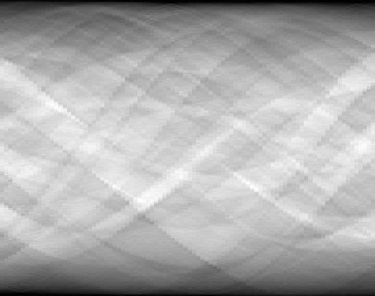
(b)

Figure 1. Clean projection and its noisy version, with $\textnormal{SNR}_{\textnormal{input}}=42.18$ dB

The image intensity range lies in $[0,x_{\max}]$, with $x_{\max}=900$. The Gaussian noise level is set to $\sigma=200$. The input signal-to-noise-ratio (SNR) in decibels (dB), between the clean projection $L\bar{x}$ and $c$ (both displayed on Figure 1) is defined as

$$\text{SNR}_{\text{input}}=20\log_{10}\left(\frac{\|L\bar{x}\|}{\|L\bar{x}-c\|}\right).$$ (6.20)

Problem (1.3) is solved using an orthonormal Symmlet basis with 4 vanishing moments, and 2 resolution levels for $W$ operator. The following penalty parameter values are chosen: $\lambda=150$, $\delta=5$, and $\alpha=0.1$. The reconstructed images using MMFBHF and MMFDRF with $10^{4}$ iterations are presented in Figure 2. We also present the results within a zoomed region-of-interest (ROI), with size $80\times 80$ pixels and circular shape, in Figure 2 (bottom). We evaluate, for each algorithm, the quantitative error between the original image $\bar{x}$ and its recovered version $\hat{x}$, through the normalized mean squared error NMSE $={\|\bar{x}-\hat{x}\|^{2}}/{\|\bar{x}\|^{2}}$, the mean absolute error MAE $=\|\bar{x}-\hat{x}\|_{\infty}$ and the SNR $=10\log_{10}\text{NMSE}$. Similar formula are used to determine SNR, MAE and NMSE scores inside the ROI. The obtained values are provided in the caption of Figure 2.

In Figure 3, we display the evolution of the SNR, along iterations and times, for codes running in MATLAB R2023a, on a laptop with AMD Ryzen 5 3550Hz, Radeon Vega Mobile Gfx, and 32 Gb RAM. One can notice that MMFBHF and MMFDRF behave similarly in terms of convergence speed. Still, all algorithms reach convergence in about $2000$ iterations, and $200$ seconds, confirming the validity of our theoretical results.

(a)

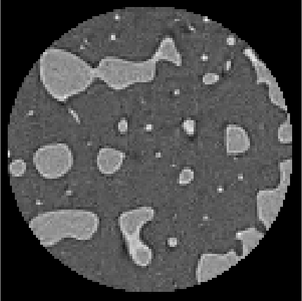
(b)

(c)

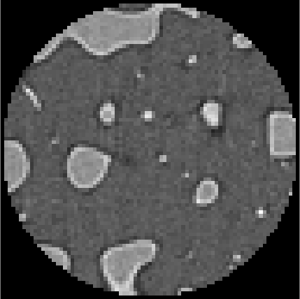
(d)

(e)

(f)

Figure 2. Original and reconstructed images (full view, and zoom) after $10^{5}$ iterations of MMFBHF and MMFDRF algorithms, respectively.

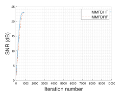
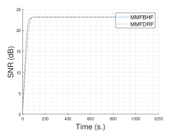
Figure 3. Evolution along iterations (left) and computational time (right) in seconds, of the SNR (in dB) between the true image and its reconstruction, for MMFBHF and MMFDRF algorithms.

7. Conclusion

In this paper, we introduced two iterative algorithms for numerically solving monotone inclusions involving the sum of a maximally $\rho$-monotone operator, a cocoercive operator, and a mismatched Lipschitzian operator. The proposed schemes can be viewed as extensions of Forward-Backward-Half-Forward and Forward-Douglas-Rachford-Forward splitting methods, that use an approximation to an adjoint operator at each iteration. We provided conditions under which the sequence generated by these variants weakly converges to a solution to the mismatched inclusion. We also showed that, under some strong monotonicity assumptions, a linear convergence rate is obtained for the two algorithms. The applicability of our study is illustrated by numerical experiments in the context of imaging of materials. When considering variational problems, the main advantage of our work with respect to [8, 10, 16, 19] is to allow dealing with mismatches on more sophisticated functions than quadratic ones.

References

- [1] H. H. Bauschke and P. L. Combettes, Convex analysis and monotone operator theory in Hilbert spaces, CMS Books in Mathematics/Ouvrages de Mathématiques de la SMC, Springer, New York, 2011, https://doi.org/10.1007/978-1-4419-9467-7.
- [2] H. H. Bauschke and P. L. Combettes, Convex analysis and monotone operator theory in Hilbert spaces, CMS Books in Mathematics/Ouvrages de Mathématiques de la SMC, Springer, Cham, second ed., 2017, https://doi.org/10.1007/978-3-319-48311-5.
- [3] H. H. Bauschke, W. M. Moursi, and X. Wang, Generalized monotone operators and their averaged resolvents, Math. Program., 189 (2021), pp. 55–74, https://doi.org/10.1007/s10107-020-01500-6.
- [4] C. Bertocchi, E. Chouzenoux, M.-C. Corbineau, J.-C. Pesquet, and M. Prato, Deep unfolding of a proximal interior point method for image restoration, Inverse Problems, 36 (2020), pp. 034005, 27, https://doi.org/10.1088/1361-6420/ab460a.
- [5] L. M. Briceño Arias and P. L. Combettes, Monotone operator methods for Nash equilibria in non-potential games, in Computational and analytical mathematics, vol. 50 of Springer Proc. Math. Stat., Springer, New York, 2013, pp. 143–159, https://doi.org/10.1007/978-1-4614-7621-4_9.
- [6] L. M. Briceño-Arias and D. Davis, Forward-backward-half forward algorithm for solving monotone inclusions, SIAM J. Optim., 28 (2018), pp. 2839–2871, https://doi.org/10.1137/17M1120099.
- [7] T. A. Bubba, M. Galinier, M. Lassas, M. Prato, L. Ratti, and S. Siltanen, Deep neural networks for inverse problems with pseudodifferential operators: An application to limited-angle tomography, SIAM Journal on Imaging Sciences, 14 (2021), pp. 470–505, https://doi.org/10.1137/20M1343075.
- [8] E. Chouzenoux, A. Contreras, J.-C. Pesquet, and M. Savanier, Convergence results for primal-dual algorithms in the presence of adjoint mismatch, SIAM Journal on Imaging Sciences, 16 (2023), pp. 1–34.
- [9] E. Chouzenoux, A. Jezierska, J.-C. Pesquet, and H. Talbot, A convex approach for image restoration with exact Poisson-Gaussian likelihood, SIAM Journal on Imaging Sciences, 8 (2015), pp. 2662–2682.
- [10] E. Chouzenoux, J.-C. Pesquet, C. Riddell, M. Savanier, and Y. Trousset, Convergence of proximal gradient algorithm in the presence of adjoint mismatch, Inverse Problems, 37 (2021), pp. Paper No. 065009, 29, https://doi.org/10.1088/1361-6420/abd85c.
- [11] E. Chouzenoux, F. Zolyniak, E. Gouillart, and H. Talbot, A majorize-minimize memory gradient algorithm applied to X-ray tomography, in Proceedings of the 20th IEEE International Conference on Image Processing (ICIP 2013), Melbourne, Australia, 15-18 Sep. 2013, pp. 1011–1015.
- [12] P. L. Combettes, Monotone operator theory in convex optimization, Math. Program., 170 (2018), pp. 177–206, https://doi.org/10.1007/s10107-018-1303-3.
- [13] P. L. Combettes and J.-C. Pesquet, Primal-dual splitting algorithm for solving inclusions with mixtures of composite, Lipschitzian, and parallel-sum type monotone operators, Set-Valued Var. Anal., 20 (2012), pp. 307–330, https://doi.org/10.1007/s11228-011-0191-y.
- [14] P. L. Combettes and J.-C. Pesquet, Fixed point strategies in data science, IEEE Transactions on Signal Processing, 69 (2021), pp. 3878–3905, https://doi.org/10.1109/TSP.2021.3069677.
- [15] L. Condat, A primal-dual splitting method for convex optimization involving Lipschitzian, proximable and linear composite terms, J. Optim. Theory Appl., 158 (2013), pp. 460–479, https://doi.org/10.1007/s10957-012-0245-9.
- [16] Y. Dong, P. C. Hansen, M. E. Hochstenbach, and N. A. Brogaard Riis, Fixing nonconvergence of algebraic iterative reconstruction with an unmatched backprojector, SIAM Journal on Scientific Computing, 41 (2019), pp. A1822–A1839, https://doi.org/10.1137/18M1206448.
- [17] Y. Dong, P. C. Hansen, M. E. Hochstenbach, and N. A. Brogaard Riis, Fixing nonconvergence of algebraic iterative reconstruction with an unmatched backprojector, SIAM Journal on Scientific Computing, 41 (2019), pp. A1822–A1839, https://doi.org/10.1137/18M1206448.
- [18] J. Eckstein and D. Bertsekas, On the Douglas-Rachford splitting method and the proximal point algorithm for maximal monotone operators, Math. Program., 55 (1992), pp. 293–318.
- [19] T. Elfving and P. C. Hansen, Unmatched projector/backprojector pairs: Perturbation and convergence analysis, SIAM Journal on Scientific Computing, 40 (2018), pp. A573–A591, https://doi.org/10.1137/17M1133828.
- [20] P. Giselsson and W. M. Moursi, On compositions of special cases of Lipschitz continuous operators, Fixed Point Theory Algorithms Sci. Eng., (2021), pp. Paper No. 25, 38, https://doi.org/10.1186/s13663-021-00709-0.
- [21] A. A. Goldstein, Convex programming in Hilbert space, Bulletin of the American Mathematical Society, 70 (1964), pp. 709 – 710, https://doi.org/bams/1183526263, https://doi.org/.
- [22] P. C. Hansen, K. Hayami, and K. Morikuni, GMRES methods for tomographic reconstruction with an unmatched back projector, tech. report, 2022, https://arxiv.org/pdf/2110.01481.pdf.
- [23] A. C. Kak and M. Slaney, Principles of Computerized Tomographic Imaging, Society of Industrial and Applied Mathematics, 2001.
- [24] E. Klann, E. T. Quinto, and R. Ramlau, Wavelet methods for a weighted sparsity penalty for region of interest tomography, Inverse Problems, 31 (2015), p. 025001.
- [25] P.-L. Lions and B. Mercier, Splitting algorithms for the sum of two nonlinear operators, SIAM J. Numer. Anal., 16 (1979), pp. 964–979, https://doi.org/10.1137/0716071.
- [26] D. A. Lorenz, S. Rose, and F. Schöpfer, The randomized Kaczmarz method with mismatched adjoint, BIT, 58 (2018), pp. 1079–1098, https://doi.org/10.1007/s10543-018-0717-x.
- [27] D. A. Lorenz and F. Schneppe, Chambolle-Pock’s primal-dual method with mismatched adjoint, Appl. Math. Optim., 87 (2023), pp. Paper No. 22, 26, https://doi.org/10.1007/s00245-022-09933-5.
- [28] I. Loris, G. Nolet, I. Daubechies, and F. A. Dahlen, Tomographic inversion using l1-norm regularization of wavelet coefficients, Geophysical Journal International, 170 (2007), pp. 359–370.
- [29] I. Loris and C. Verhoeven, On a generalization of the iterative soft-thresholding algorithm for the case of non-separable penalty, Inverse Problems, 27 (2011), pp. 125007, 15, https://doi.org/10.1088/0266-5611/27/12/125007.
- [30] Y. Malitsky and M. K. Tam, A forward-backward splitting method for monotone inclusions without cocoercivity, SIAM J. Optim., 30 (2020), pp. 1451–1472, https://doi.org/10.1137/18M1207260.
- [31] Y. Marnissi, Y. Zheng, E. Chouzenoux, and J.-C. Pesquet, A variational bayesian approach for image restoration. application to image deblurring with Poisson-Gaussian noise., IEEE Transactions on Computational Imaging, 3 (2017), pp. 722–737.
- [32] G. Passty, Ergodic convergence to a zero of the sum of monotone operators in hilbert space, J. Math. Anal. Appl., 72 (1979), pp. 383–390.
- [33] N. Pustelnik, A. Benazza-Benhayia, Y. Zheng, and J.-C. Pesquet, Wavelet-based image deconvolution and reconstruction, Wiley Encyclopedia of Electrical and Electronics Engineering, 2016, pp. 1–34.
- [34] E. K. Ryu and B. C. Vũ, Finding the forward-Douglas-Rachford-forward method, J. Optim. Theory Appl., 184 (2020), pp. 858–876, https://doi.org/10.1007/s10957-019-01601-z.
- [35] M. Savanier, E. Chouzenoux, J.-C. Pesquet, and C. Riddell, Unmatched preconditioning of the proximal gradient algorithm, IEEE Signal Processing Letters, 29 (2022), pp. 1122–1126, https://doi.org/10.1109/LSP.2022.3169088.
- [36] M. Savanier, E. Chouzenoux, J.-C. Pesquet, and C. Riddell, Deep unfolding of the dbfb algorithm with application to roi ct imaging with limited angular density, IEEE Transactions on Computational Imaging, 9 (2023), pp. 502–516, https://doi.org/10.1109/TCI.2023.3279053.
- [37] P. Tseng, A modified forward-backward splitting method for maximal monotone mappings, SIAM J. Control Optim., 38 (2000), pp. 431–446, https://doi.org/10.1137/S0363012998338806.
- [38] B. C. Vũ, A splitting algorithm for dual monotone inclusions involving cocoercive operators, Adv. Comput. Math., 38 (2013), pp. 667–681, https://doi.org/10.1007/s10444-011-9254-8.
- [39] W. van Aarle, W. J. Palenstijn, J. Cant, E. Janssens, F. Bleichrodt, A. Dabravolski, J. D. Beenhouwer, K. J. Batenburg, and J. Sijbers, Fast and flexible x-ray tomography using the astra toolbox, Opt. Express, 24 (2016), pp. 25129–25147, https://doi.org/10.1364/OE.24.025129.
- [40] W. van Aarle, W. J. Palenstijn, J. De Beenhouwer, T. Altantzis, S. Bals, K. J. Batenburg, and J. Sijbers, The astra toolbox: A platform for advanced algorithm development in electron tomography, Ultramicroscopy, 157 (2015), pp. 35–47, https://doi.org/https://doi.org/10.1016/j.ultramic.2015.05.002.
- [41] F. Xu and K. Mueller, A comparative study of popular interpolation and integration methods for use in computed tomography, in Proceedings of the 3rd IEEE International Symposium on Biomedical Imaging: Nano to Macro, 2006., Apr 2006, pp. 1252–1255.
- [42] L. Zanni, A. Benfenati, M. Bertero, and V. Ruggiero, Numerical methods for parameter estimation in poisson data inversion, Journal of Mathematical Imaging and Vision, 52 (2015), pp. 397––413.
- [43] G. Zeng and G. Gullberg, A ray-driven backprojector for backprojection filtering and filtered backprojection algorithms, in 1993 IEEE Conference Record Nuclear Science Symposium and Medical Imaging Conference, 1993, pp. 1199–1201, https://doi.org/10.1109/NSSMIC.1993.701833.
- [44] G. Zeng and G. Gullberg, Unmatched projector/backprojector pairs in an iterative reconstruction algorithm, IEEE Transactions on Medical Imaging, 19 (2000), pp. 548–555, https://doi.org/10.1109/42.870265.
- [45] G. Zeng and G. Gullberg, Unmatched projector/backprojector pairs in an iterative reconstruction algorithm, IEEE Transactions on Medical Imaging, 19 (2000).