Antenna Response Consistency Driven Self-supervised Learning for WIFI-based Human Activity Recognition.

Abstract

Self-supervised learning (SSL) for WiFi-based human activity recognition (HAR) holds great promise due to its ability to address the challenge of insufficient labeled data. However, directly transplanting SSL algorithms, especially contrastive learning, originally designed for other domains to CSI data, often fails to achieve the expected performance. We attribute this issue to the inappropriate alignment criteria, which disrupt the semantic distance consistency between the feature space and the input space. To address this challenge, we introduce Antenna Response Consistency (ARC) as a solution to define proper alignment criteria. ARC is designed to retain semantic information from the input space while introducing robustness to real-world noise. Moreover, we substantiate the effectiveness of ARC through a comprehensive set of experiments, demonstrating its capability to enhance the performance of self-supervised learning for WiFi-based HAR by achieving an increase of over 5% in accuracy in most cases and achieving a best accuracy of 94.97%.

Keywords Self-supervised Learning  $\cdot$ Channel State Information  $\cdot$ Wireless Sensing

1 Introduction

Human activity recognition (HAR) is of significant importance across a range of human-centric applications. These applications encompass health monitoring for elderly individuals living alone, facilitating human-device interactions within smart home environments, and enhancing the immersive experience of virtual reality gaming. Compared to traditional HAR methods employing cameras, wearable devices, and radar, CSI-based approaches have garnered significant attention from researchers due to their cost-effectiveness and privacy-friendly characteristics. CSI-based techniques ubiquitous commercial off-the-shelf (COTS) devices within home environments, devoid of visual data, thereby safeguarding the privacy concerns of individuals wary of video surveillance.

There are some research works in CSI-based HAR which can be categorized into learning-based methods and model-based methods. Learning-based methods in CSI-based HAR involve the extraction of statistical features from CSI signals, and this can be done through the hand-crafted way or deep learning approach. However, a significant limitation of these methods is their substantial demand for labeled CSI data. Labeling CSI data is a challenging task because raw CSI data is not interpretable by humans, making the labeling both cumbersome and expensive. On the other hand, model-based methods aim to construct a physical model that maps wireless signals to human movement. A recent work, Widar3.0 [1], introduces a zero-effort model, signifying that no additional data collection efforts are required when deploying the model in a new environment. However, Widar3.0 requires the target environment to be equipped with more than three receivers, and its high computational complexity for feature extraction poses a barrier to its application in real-time scenarios.

Self-supervised learning (SSL) is a promising approach that trains models using cost-effective unlabeled CSI data to overcome the limitation of insufficient labeled CSI data. SSL has achieved significant success in computer vision and natural language processing tasks, a recent systematic study [2] has revealed that directly applying SSL methods developed for other research domains to CSI signal data does not yield the expected performance. For example, it has been demonstrated that contrastive learning, a prevalent SSL paradigm, can outperform its supervised counterpart in computer vision [3], but it performs poorly on CSI datasets [2].

This discrepancy can be attributed to the fact that the existing augmentation functions, originally tailored for other domains, do not yield an appropriate definition of Alignment for the feature space of CSI data. Existing work [4] highlights that the objective of contrastive learning is to learn a feature space with optimal uniformity and alignment. Uniformity requires the distribution of the feature space to be as close to a uniform distribution as possible. The rationale behind uniformity stems from an information theory perspective. It posits that the closer the feature distribution is to a uniform distribution, the more information the features retain from the input. Alignment implies that similar examples should be close in the feature space. The process of "bringing positive pairs closer together while pushing negative pairs farther apart" in contrastive learning effectively optimizes both alignment and uniformity in the feature space.

Indeed, while alignment intuitively relates to improving the classification of similar examples, the real challenge lies in establishing an appropriate definition of similarity that aligns with the real distribution of CSI data. Specifically, augmented views generated using transformation functions designed for images or other types of data may never occur in a real device. For instance, consider the simple example of rotating an image, which aligns with the actual distribution of images since it’s plausible for a photographer to capture images after rotating the camera. However, it is practically impossible for real-world WiFi devices to produce rotated CSI data. Therefore, the alignment criteria learned from such transformations cannot offer accurate guidance on "which CSI data should be considered similar," and, in fact, may prove counterproductive for downstream CSI-based tasks.

For this problem, we propose Antenna Response Consistency (ARC) for CSI-based SSL, which utilize the inherent consistency among different antennas to define the alignment criteria.

Figure 1: The identical human action exhibits distinct propagation paths across multiple antennas.

Existing research efforts [5, 6] underscores that variations in propagation path, antenna directivity, and other factors lead to distinct recordings of the same action when captured by different antennas (As Figure 1 shows). These variations can be characterized within the CSI data model as amplitude attenuation and phase shifts. The diverse records from different antennas can be naturally utilized as similar views of the original recordings, as they are consistent in both spatial and temporal semantic, aiding in the learning of suitable alignment criteria for CSI data. Although our method is based on the theory constructed for contrastive learning, we find out it is also suitable for other SSL paradigms like autoencoder. The process of "reconstructing from the (corrupted) input" in autoencoder [7, 8] is akin to maximizing uniformity, aiming to preserve as much information as possible. Incorporating ARC into autoencoder algorithms such as MAE enables the model to learn a feature space with improved alignment and subsequently achieve higher performance.

In summary, our contributions encompass:

1) We integrate domain knowledge of CSI data into self-supervised learning (SSL) algorithms through the introduction of ARC. This approach enhances SSL for CSI-based tasks by enabling accurate learning of alignment within the feature space.

2) The effectiveness of ARC was analyzed from two perspectives: CSI data structure and feature learning.

3) Through extensive experimentation, we have provided compelling evidence that demonstrates the effectiveness of ARC in improving the performance of SSL algorithms for CSI data.

2 Related Work

2.1 CSI-based Sensing

Researchers have proposed a variety of methods for addressing CSI-based HAR task. Existing work on CSI-based sensing can be categorized into two types: model-based algorithms and learning-based algorithms. Model-based algorithms entail the establishment of a mapping from signals to motion through the utilization of a physical model. Fresnel Zone divide the space between and around the transmitter and the receiver into concentric prolate ellipsoidal regions, or Fresnel Zone. Fresnel Zone shed a light of how signal propagate and deflect off between transmitter and receiver. [9] for the first time based on Fresnel Zone proposed a phase-based method to inference the walking direction of users. [10] conducted further examinations of the properties of the Fresnel reflection model for human sensing. [11] introduce "MultiSense" that utilizes Fresnel zone with common Wi-Fi devices to enable multi-person breathing monitoring. More recently, [12] proposed a dynamic Fresnel model to address the gaps in theoretical models based on mobile receivers.

Another branch of research within model-based algorithms centers on harnessing the Doppler effect, which results in a shift in the observed signal frequency known as Doppler frequency shift (DFS). The primary cause of DFS is the alteration in the length of the signal propagation path, a phenomenon directly influenced by human activities. DFS serves as an effective model for tasks like motion detection and speed estimation. In the work by Pu et al. [13], WiSee is introduced as a system that extracts DFS and calculates its power to enable whole-home sensing and the recognition of human gestures. Widar [14] focuses on constructing a path length change rate model based on DFS, geometrically quantifying the relationships between CSI dynamics and the user’s location and velocity. In the study by Li et al. [15], IndoTrack is presented, combining both DFS and Angle of Arrival (AoA) for indoor human tracking. It introduces a novel MUSIC-based algorithm called Doppler-MUSIC for estimating Doppler velocity. Widar’s subsequent project, Widar2.0 [16], develops a system that leverages the EM algorithm to estimate multi-dimensional signal parameters, including DFS, using only a single wireless link. In [1], a novel feature called the body-coordinate velocity profile, based on DFS, is proposed for zero-effort cross-domain gesture recognition.

2.2 Self-supervised Learning for CSI-data

Self-supervised learning (SSL) has emerged as a promising alternative to supervised learning, garnering significant attention for its data efficiency and generalization capabilities. Many state-of-the-art models have adopted this paradigm. A typical application framework for SSL involves two main steps. First, the model is trained on an unlabeled dataset using SSL algorithms. Second, the model, or specifically the classifier, is fine-tuned on a much smaller labeled dataset. This two-step process is commonly referred to as a "pretrain-then-finetune" procedure. In the machine learning community, there are four popular types of SSL algorithms: instance-instance contrast, context-instance contrast, and autoencoder-based methods. Instance-instance contrastive algorithms, such as SimCLR [17], MoCo [3], and SwAV [18], directly investigate the relationships between instance-level local representations of different samples. A common form to learning the relationship between different samples is to simultaneously generate two noisy versions of a single anchor instance. The goal is to maximize the similarity between the representations of these two augmented versions while minimizing the similarity between the augmented versions of different instances. Context-instance contrast, as demonstrated in works like [19] and [20], centers around modeling the relationship between the local features of a sample and its global context representation. The primary objective of autoencoding models is to reconstruct input from (corrupted) input data, such as MAE[7].

In recent years, SSL for CSI-based HAR has also been developing vigorously. For instance, in [21], a contrastive learning paradigm is employed to extract semantic features from two views of raw signal data and Scalgram representations. Researchers have been exploring frequency-domain data augmentation techniques in addition to existing time-domain augmentation during self-supervised training, as highlighted in [22]. Furthermore, [23] enables the learning of high-level features through various original auxiliary tasks, eliminating the need for labor-intensive labeling processes. As a form of multivariate time series data, CSI shares similarities with general multivariate time series data. Recent research has shown that state-of-the-art methods originally designed for SSL on general multivariate time series data, such as TS2Vec [24], have been proven to outperform their standard counterparts like SimCLR when applied to CSI data.

3 Method

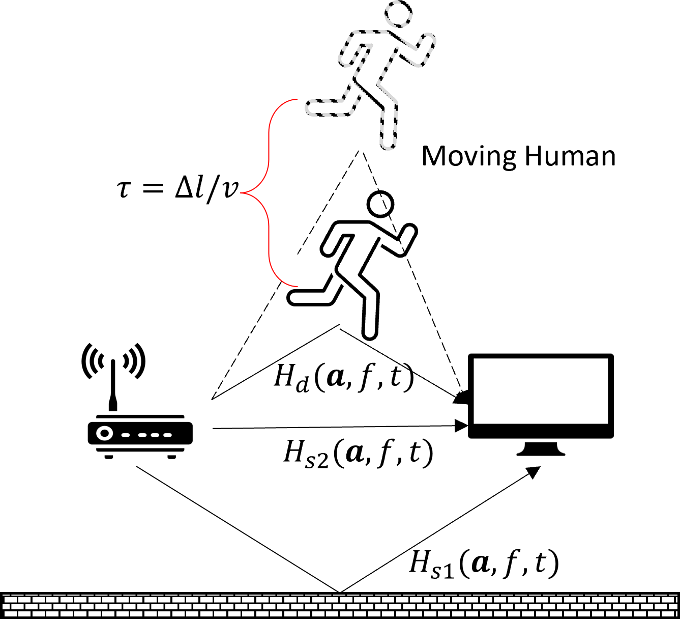
Figure 2: Human movement at speed $v$ results in variations in the path length $\Delta l$ for the reflected signal.

First and foremost, we would like to provide a brief introduction to the format of CSI data. In a WiFi system utilizing MIMO-OFDM, the Channel State Information (CSI) is typically represented as a four-dimensional (4D) tensor, denoted as $\mathbf{H}\in\mathbb{C}^{N\times M\times K\times T}$. In this notation, $N$, $M$, $K$, and $T$ correspond to the number of receiver antennas, transmit antennas, subcarriers, and packets, respectively. Concurrently, the categories of human actions are represented as $y\in\mathbb{R}$. Considering the influence of multi-path effects, the measured CSI for the $\mathbf{a}$th transmitter-receiver (Tx-Rx) antenna pair, $f$th subcarriers, and $t$th packet can be mathematically described as shown in Equation 1.

$$\mathbf{H}(\mathbf{a},f,t)=(\mathbf{H}_{s}(\mathbf{a},f,t)+\mathbf{H}_{d}(\mathbf{a},f,t))e^{-j2\pi\epsilon(f,t)}=(\mathbf{H}_{s}(\mathbf{a},f,t)+\sum_{l}^{L}{\alpha_{l}(\mathbf{a},f,t)e^{-j2\pi\tau_{l}(f,t)}})e^{-j2\pi\epsilon(f,t)}$$ (1)

In Equation 1, the received CSI tensor is decomposed into two components. $H_{s}$ represents the constant component arising from all static paths (as the $H_{s1}$ and $H_{s2}$ in Figure 2), while $H_{d}$ represents the sum of dynamic paths (as the $H_{d}$ in Figure 2). In this equation, $\alpha_{l}(\mathbf{a},f,t)$ and $\tau_{l}(f,t)$ denote the amplitude attenuation and propagation delay of the $l$th path, respectively. $\epsilon(f,t)$ accounts for the phase offset resulting from cyclic shift diversity and sampling offset. This parameter remains consistent across all antennas within the same device, as discussed in [5].

3.1 Alignment Criteria For CSI Data

Alignment in this context pertains to the requirement that two samples forming a positive pair should be mapped to nearby features, ensuring that they are mostly invariant to irrelevant noise factors [4]. The central challenge lies in defining positive pair examples.

To elaborate, let’s consider an augmentation function denoted as $G(\cdot)$, which generates an augmented view of the input $\mathbf{H}$, represented as $G(\mathbf{H})$. Given that models trained via SSL aim to map positive pairs to nearby features, we desire that the positive pair ${\mathbf{H},G(\mathbf{H})}$ belongs to the same class. This way, a straightforward measure, such as the Euclidean distance, in the feature space can approximate the "semantic" distance in the input space. We refer to this concept as Semantic Information Retention.

Emphasizing the significance of Semantic Information Retention, let’s contemplate a scenario in which the transformation function alters the category of the input data, indicating that we have $P(y|\mathbf{H})\neq P(y|G(\mathbf{H}))$. Consider a model denoted as $F(\cdot)$ that adheres to the alignment requirement and maps input $\mathbf{H}$ to a feature vector $F(\mathbf{H})$.

In the context of a linear regression classifier expressed as $\min\sum\|y-(wF(\mathbf{H})+b)\|^{2}$, it performs classification using the feature vector $F(\mathbf{H})$ by minimizing the sum of squared residuals between the ground truth class $y$ and the linear mapping $wF(\mathbf{H})+b$.

If we denote a model with ideal alignment properties as $F^{*}$, we can express this as $\lim_{F\to F^{*}}\|w(F(\mathbf{H})-F(G(\mathbf{H})))\|^{2}=0$. This suggests that, as the model approaches ideal alignment, the classifier will classify $\mathbf{H}$ and $G(\mathbf{H})$ as the same class. However, this contradicts the ground truth and can be detrimental to model performance.

Furthermore, real-world noise that the model should encounter aligns with what is commonly experienced in real-world data, a concept we term as Real-world Noise Invariance. For instance, noise introduced by rotating CSI data is never encountered in actual devices, and accounting for it is not conducive to model robustness.

3.2 Antenna Response Consistency

In this section, let us closely examine the dynamic path term in Equation 1.

$$\mathbf{H}_{d}(\mathbf{a},f,t)\\ =\sum_{l}^{L}{\alpha_{l}(\mathbf{a},f,t)e^{-j2\pi\tau_{l}(f,t)}}$$ (2)

it is noteworthy that $\alpha_{l}(\mathbf{a},f,t)$ is closely linked to the antenna configuration within the same device. As shown in Figure 2, $\tau_{l}(f,t)$ reflects the propagation delay induced by changes in path length, which can be viewed as a function of human activities. The distinct antennas within the same device experience the dynamic path caused by the same human activity. The Antenna Response Consistency (ARC) can be mathematically articulated:

$$F^{*}(\mathbf{H}(\mathbf{a}_{q},f,t))=F^{*}(\mathbf{H}(\mathbf{a}_{k},f,t))=\tau_{l}(f,t)$$ (3)

$F^{*}$ denotes the ideal mapping from the distinct antenna $\mathbf{a}_{q}$ and $\mathbf{a}_{k}$ response of the CSI signal, $\mathbf{H}$, to the propagation delay induced by human activity, $\tau_{l}(f,t)$. Accordingly, we introduce an objective function rooted in ARC:

$$J=Sim(F(\mathbf{H}(\mathbf{a}_{q},f,t)),F(\mathbf{H}(\mathbf{a}_{k},f,t)))$$ (4)

The model $F$ should be trained to maximize the objective function $J$, aiming to maximize the similarity between the features $F(\mathbf{H}(\mathbf{a}_{q},f,t))$ and $F(\mathbf{H}(\mathbf{a}_{k},f,t))$.

We have elucidated the core idea of ARC. Importantly, we wish to underscore that ARC can be seamlessly incorporated into existing SSL algorithms with just a few lines of code, offering the model appropriate alignment criteria for CSI data. In the context of contrastive learning, the algorithm framework and loss function are instrumental in acquiring a feature space characterized by alignment and uniformity, with alignment criteria defined by the transformation function. Capitalizing on this characteristic, we seamlessly incorporate ARC into contrastive learning by treating different antennas as distinct augmented views. Algorithm 1 presents the pseudocode for integrating ARC into the widely-used contrastive learning algorithm MoCo. Figure 3(a) illustrates the framework of MoCo-ARC.

Autoencoder, another SSL paradigm, maximizes the uniformity by reconstructing the input. We integrate the ARC to autoencoder by maximizing the cosine similarity of different antenna. Algorithm 2 presents the pseudocode for integrating ARC into MAE. Figure 3(b) illustrates the framework of MAE-ARC.

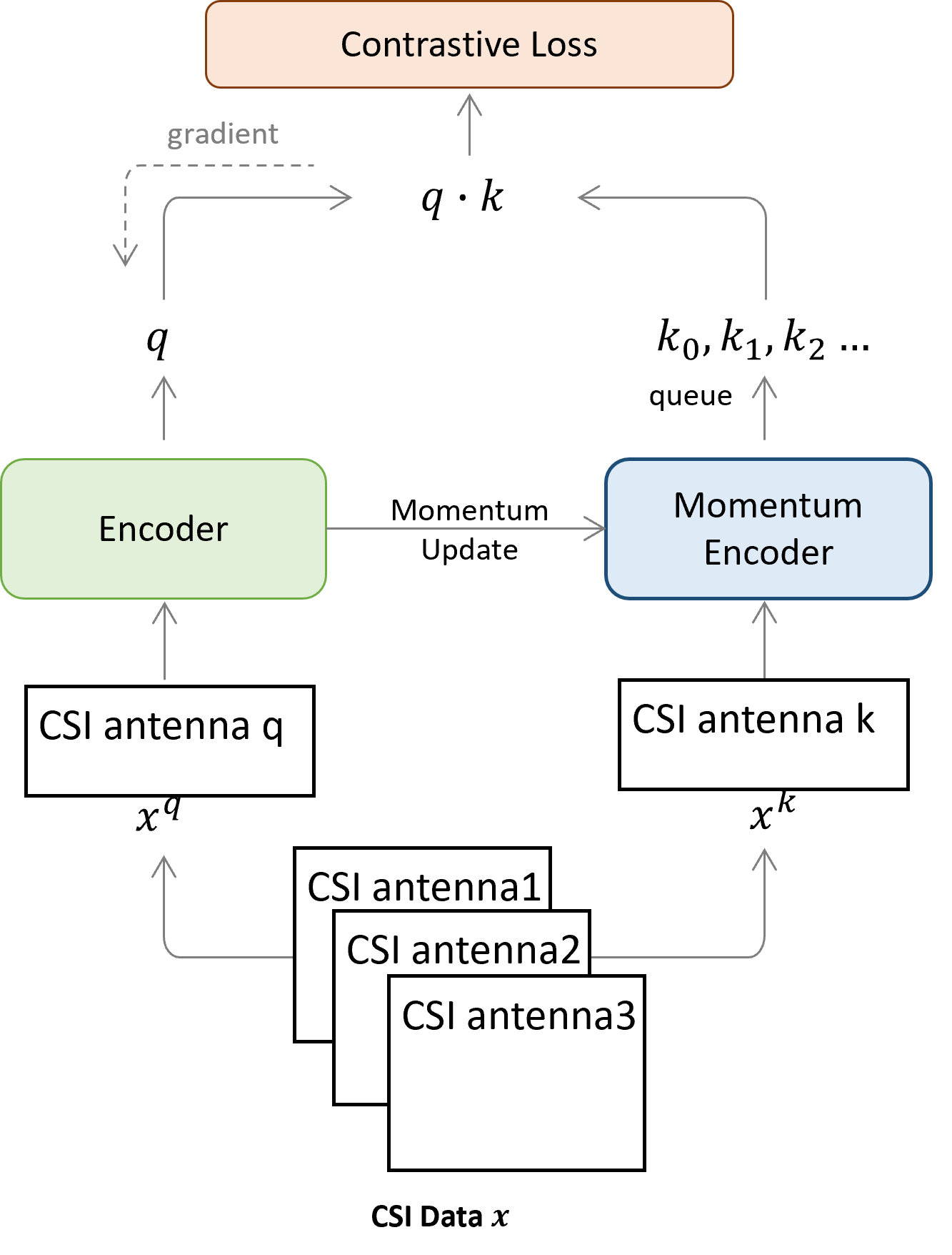
(a) MoCo-ARC

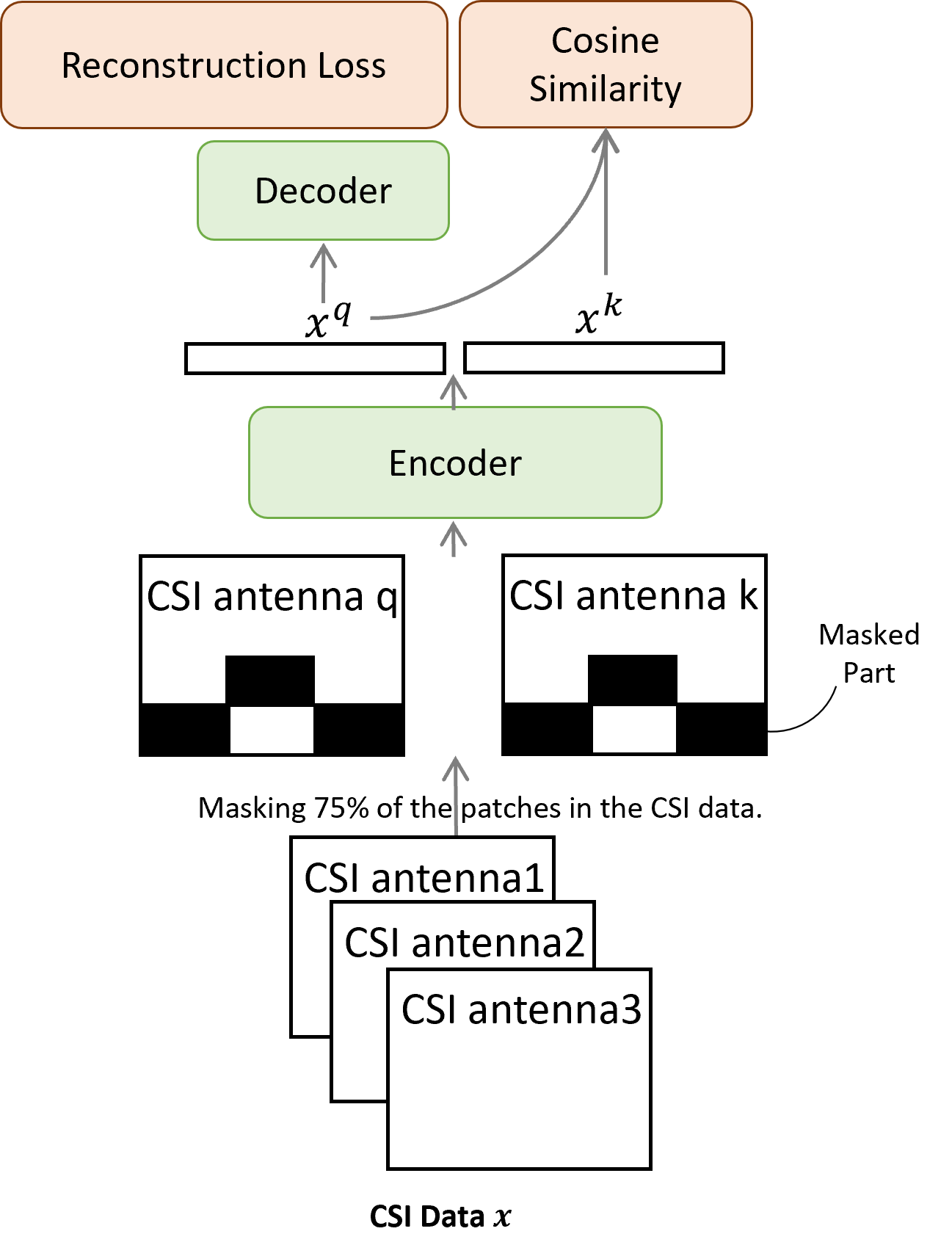
(b) MAE-ARC

Figure 3: Frameworks of MoCo-ARC and MAE-ARC. (a)MoCo-ARC: Two antennas are randomly chosen from the input CSI signal, denoted as $x^{q}$ and $x^{k}$, to serve as the two augmented views of contrastive learning. (b)MAE-ARC: A random mask is applied to the input, and then two antennas, $q$ and $k$, are selected randomly to serve as inputs for the encoder. Subsequently, the feature $x^{q}$ is reconstructed through the decoder, and the reconstruction loss is calculated. Additionally, the ARC loss between $x^{q}$ and $x^{k}$, quantified as their cosine similarity, is also computed.

Algorithm 1 Pseudocode of MoCo-ARC in a Python-like style.

1:function MoCo-ARC($\mathbf{H},F_{a},F_{p}$)$\triangleright$ Where $\mathbf{H}={\mathbf{H}_{a1},\mathbf{H}_{a2},\mathbf{H}_{a3}}$; $F_{a},F_{p}$-amplitude and phase encoder

2:     for $\mathbf{H}$ in Dataloader do

3:         Random generate three int $q,k,ref$

4:         $\mathbf{H}_{q},\mathbf{H}_{k},\mathbf{H}_{ref}$ = AntennaSelection($\mathbf{H},(q,k,ref)$)

5:         $A_{q},A_{k}$ = np.abs($\mathbf{H}_{q}$),np.abs($\mathbf{H}_{k}$) $\triangleright$ Amplitude part

6:         $z_{aq},z_{ak}$ = $F_{a}$($A_{q}$),$F_{a}$($A_{k}$)

7:         $loss_{a}$ = InfoNCE($z_{aq},z_{ak}$)

8:         $\mathbf{C}_{q},\mathbf{C}_{k}=\mathbf{H}_{q}*\widetilde{\mathbf{H}}_{ref},\mathbf{H}_{k}*\widetilde{\mathbf{H}}_{ref}$ $\triangleright$ Phase part

9:         $P_{q},P_{k}$ = np.angle($\mathbf{C}_{q}$),np.angle($\mathbf{C}_{k}$)

10:         $z_{pq},z_{pk}$ = $F_{p}$($P_{q}$),$F_{p}$($P_{k}$)

11:         $loss_{p}$ = InfoNCE($z_{pq},z_{pk}$)

12:         $loss$ = $loss_{a}+loss_{p}$

13:     end for

14:end function

Algorithm 2 Pseudocode of MAE-ARC in a Python-like style.

1:function MAE-ARC($\mathbf{H},F_{a},F_{p},D_{a},D_{p}$)$\triangleright$ Where $\mathbf{H}={\mathbf{H}_{a1},\mathbf{H}_{a2},\mathbf{H}_{a3}}$; $D_{a},D_{p}$-amplitude and phase decoder

2:     for $\mathbf{H}$ in Dataloader do

3:         Random generate three int $q,k,ref$

4:         $\mathbf{H}_{q},\mathbf{H}_{k},\mathbf{H}_{ref}$ = AntennaSelection($\mathbf{H},(q,k,ref)$)

5:         $A_{q},A_{k}$ = np.abs($\mathbf{H}_{q}$),np.abs($\mathbf{H}_{k}$) $\triangleright$ Amplitude part

6:         $z_{aq},z_{ak}$ = $F_{a}$($A_{q}$),$F_{a}$($A_{k}$)

7:         $\hat{A}_{q}$ = $D_{a}$($z_{aq}$) $\triangleright$ Reconstruction

8:         $loss_{a}$ = MSE($\hat{A}_{q},A_{q}$)+alpha*cos_similarity($z_{aq},z_{ak}$)

9:         $\mathbf{C}_{q},\mathbf{C}_{k}=\mathbf{H}_{q}*\widetilde{\mathbf{H}}_{ref},\mathbf{H}_{k}*\widetilde{\mathbf{H}}_{ref}$ $\triangleright$ Phase part

10:         $P_{q},P_{k}$ = np.angle($\mathbf{C}_{q}$),np.angle($\mathbf{C}_{k}$)

11:         $z_{pq},z_{pk}$ = $F_{p}$($P_{q}$),$F_{p}$($P_{k}$)

12:         $\hat{P}_{q}$ = $D_{p}$($z_{pq}$) $\triangleright$ Reconstruction

13:         $loss_{p}$ = MSE($\hat{P}_{q},P_{q}$)+alpha*cos_similarity($z_{pq},z_{pk}$)

14:         $loss$ = $loss_{a}+loss_{p}$

15:     end for

16:end function

3.3 Justification

Responses from different antennas of the same device can be considered interrelated. They naturally fulfill the requirements of "Semantic Information Retention" and "Real-world Noise Invariance."

Firstly, it is evident that the different antenna responses of the same device belong to the same action class, meaning that $P(y|\mathbf{H}(\mathbf{a}_{i}))=P(y|\mathbf{H}(\mathbf{a}_{j}))$.

Secondly, ARC enhances the model’s robustness to noise caused by static paths and amplitude attenuation. Popular models like CNN or Transformer cannot process complex inputs, so we split the input into amplitude and phase components. By omitting $f$, $t$, and the constant component in Equation 1, we obtain Equation 5.

$$\mathbf{H}(\mathbf{a}) =(\mathbf{H}_{s}(\mathbf{a})+\sum_{l}^{L}{\alpha_{l}(\mathbf{a})e^{-j\tau_{l}}})e^{-j\epsilon}$$ (5)

$$=(\mathcal{Re}\mathbf{H}_{s}(\mathbf{a})+j\mathcal{Im}\mathbf{H}_{s}(\mathbf{a})+\sum_{l}^{L}{\alpha_{l}(\mathbf{a})(\cos(\tau_{l})-j\sin(\tau_{l}))})e^{-j\epsilon}$$

$$=(\mathcal{Re}\mathbf{H}_{s}(\mathbf{a})+\sum_{l}^{L}{\alpha_{l}(\mathbf{a})\cos(\tau_{l})}+j(\mathcal{Im}\mathbf{H}_{s}(\mathbf{a})-\sum_{l}^{L}{\alpha_{l}(\mathbf{a})\sin(\tau_{l})}))e^{-j\epsilon}$$

Amplitude

Following the principles of complex number arithmetic, when a complex number is multiplied by another complex number with an amplitude of 1, it does not affect its amplitude. Therefore, the amplitude of the input $\mathbf{H}$ is provided in Equation 6.

$$\mathcal{Amp}\mathbf{H}(\mathbf{a}) =\mathcal{Amp}(\mathcal{Re}\mathbf{H}_{s}(\mathbf{a})+\sum_{l}^{L}{\alpha_{l}(\mathbf{a})\cos(\tau_{l})}+j(\mathcal{Im}\mathbf{H}_{s}(\mathbf{a})-\sum_{l}^{L}{\alpha_{l}(\mathbf{a})\sin(\tau_{l})}))$$ (6)

$$=((\mathcal{Re}\mathbf{H}_{s}(\mathbf{a})+\sum_{l}^{L}{\alpha_{l}(\mathbf{a})\cos(\tau_{l})})^{2}+(\mathcal{Im}\mathbf{H}_{s}(\mathbf{a})-\sum_{l}^{L}{\alpha_{l}(\mathbf{a})\sin(\tau_{l})})^{2})^{\frac{1}{2}}$$

The amplitude of input data can be regard as a function $A(\mathbf{a},\boldsymbol{\tau})=\mathcal{Amp}\mathbf{H}(\mathbf{a})$, which is only related to the Tx-Rx antenna pairs $\mathbf{a}$ and the propagation delay $\boldsymbol{\tau}$ of dynamic paths. Given two random Tx-Rx antenna pairs $\mathbf{a}_{q}$ and $\mathbf{a}_{k}$, utilizing the square of $l^{2}$-norm of the feature difference between the two antenna pairs to quantify the similarity, the ARC objective function for amplitude can be formed as:

$$\operatorname*{argmin}_{F}\|F(A(\mathbf{a}_{q},\boldsymbol{\tau})-F(A(\mathbf{a}_{k},\boldsymbol{\tau}))\|^{2}\geq\|f(\boldsymbol{\tau})-f(\boldsymbol{\tau})\|^{2}=0$$ (7)

Certainly, the objective function has a lower bound of 0. This minimum value is reached when the model $F$ maps the input amplitude to an injective function $f$ of the path change $\boldsymbol{\tau}$ caused by human activities.

Phase

Similarly, in accordance with the principles of complex number arithmetic, multiplying a complex number by another complex number with an amplitude of 1 is equivalent to rotating it by a specific angle, as demonstrated in Equation 8.

$$\mathcal{Phase}\mathbf{H}(\mathbf{a}) =\mathcal{Phase}(\mathbf{H}_{s}(\mathbf{a})+\sum_{l}^{L}{\alpha_{l}(\mathbf{a})e^{-j\tau_{l}}})-\epsilon$$ (8)

$$=\arctan(\frac{\mathcal{Im}\mathbf{H}_{s}(\mathbf{a})-\sum_{l}^{L}{\alpha_{l}(\mathbf{a})\sin(\tau_{l})}}{\mathcal{Re}\mathbf{H}_{s}(\mathbf{a})+\sum_{l}^{L}{\alpha_{l}(\mathbf{a})\cos(\tau_{l})}})-\epsilon$$

Minimizing $\|F(\mathcal{Phase}\mathbf{H}(\mathbf{a}_{q}))-F(\mathcal{Phase}\mathbf{H}(\mathbf{a}_{k}))\|^{2}$ can lead the model to learn the phase offset pattern rather than the CSI signal itself. For any $\mathbf{a}$, the lower bound $\|F(\mathcal{Phase}\mathbf{H}(\mathbf{a}_{q}))-F(\mathcal{Phase}\mathbf{H}(\mathbf{a}_{k}))\|^{2}\geq 0$ can be achieved when $F(\mathcal{Phase}\mathbf{H}(\mathbf{a}))=f(\epsilon)$. This assertion is grounded in the explanation provided in Section 3, where it is established that $\epsilon$ remains consistent across all antennas within the same device.

Therefore, we employ the conjugate multiplication step, a technique widely used in previous works [25, 14, 15], to eliminate the phase offset $\epsilon$. Specifically, we select an Tx-Rx antenna pair, denoted as $\mathbf{a}_{ref}$, as the reference antenna pair and calculate the conjugate multiplications between the CSIs of $\mathbf{a}_{ref}$ and the remaining antenna pairs, as shown in Equation 9.

$$\mathbf{H}(\mathbf{a})*\widetilde{\mathbf{H}}(\mathbf{a}_{ref}) =(\mathbf{H}_{s}(\mathbf{a})+\sum_{l}^{L}{\alpha_{l}(\mathbf{a})e^{-j\tau_{l}}})e^{-j\epsilon}*(\widetilde{\mathbf{H}_{s}}(\mathbf{a}_{ref})+\sum_{l}^{L}{\alpha_{l}(\mathbf{a}_{ref})e^{j\tau_{l}}})e^{j\epsilon}$$ (9)

$$=(\mathbf{H}_{s}(\mathbf{a})+\sum_{l}^{L}{\alpha_{l}(\mathbf{a})e^{-j\tau_{l}}})*(\widetilde{\mathbf{H}_{s}}(\mathbf{a}_{ref})+\sum_{l}^{L}{\alpha_{l}(\mathbf{a}_{ref})e^{j\tau_{l}}})$$

The phase of $\mathbf{H}(\mathbf{a})*\widetilde{\mathbf{H}}(\mathbf{a}{\text{ref}})$ can be expressed as a function of $\mathbf{a}$ and $\boldsymbol{\tau}$, denoted as $P(\mathbf{a},\boldsymbol{\tau})=\mathcal{Phase}(\mathbf{H}(\mathbf{a})*\widetilde{\mathbf{H}}(\mathbf{a}{\text{ref}}))$. The specific antenna pair $\mathbf{a}_{\text{ref}}$ is omitted, as it remains the same for all $\mathbf{a}$. The ARC objective function for phase can be formed as:

$$\operatorname*{argmin}_{F}\|F(P(\mathbf{a}_{q},\boldsymbol{\tau}))-F(P(\mathbf{a}_{k},\boldsymbol{\tau}))\|^{2}\geq\|f(\boldsymbol{\tau})-f(\boldsymbol{\tau})\|^{2}=0$$ (10)

The lower bound is achieved when the model $F$ maps the input phase to $f(\boldsymbol{\tau})$.

Based on the analysis provided earlier, applying ARC to both amplitude and phase allows the model to extract feature of dynamic path length variations $\boldsymbol{\tau}$ from the raw input. This variation in dynamic paths is solely associated with human actions when there are no other moving objects. Consequently, the application of ARC retains the most important semantic information.

Furthermore, by examining Equations 6, 7, 9, and 10, it’s evident that ARC enables the model to map CSI data (both amplitude and phase) with varying static path signals $\mathbf{H}_{s}$ and amplitude fading $\alpha(\mathbf{a})$ to nearby locations in the feature space. This demonstrates the model’s robustness to noise originating from static paths and amplitude fading.

In summary, ARC fulfills both the criteria of retaining semantic information and being invariant to real-world noise.

4 Experiments

All experiments were performed on Nvidia RTX 3080 GPUs, and we adopted the hyperparameter settings outlined in [2]. We use accuracy to evaluate the model performance. Other detail of experiments are given as follows:

4.1 Baseline

Widar3.0

[1] is designed to derive and extract domain-independent features of human gestures at a lower signal level. These features represent the unique kinetic characteristics of gestures and are not specific to any particular domain. Building on this foundation, Widar3.0 has developed a deep neural network for gesture classification. Therefore, widar is a hybrid algorithm that combines model-based and learning-based methods.

We have also chosen the following self-supervised learning algorithm as a baseline to compare the performance before and after incorporating ARC. This comparison will showcase the overall effectiveness of our method across different SSL algorithms.

MoCo

as introduced by [3], utilizes contrasting differently augmented views of a given input example to enhance representation learning. This algorithm incorporates a momentum encoder and a queue to construct a dynamic dictionary. Thanks to this dictionary, MoCo enables the utilization of more negative pairs without requiring additional GPU memory.

MAE

[7] utilizes a masked reconstruction loss function to encourage the model to learn a sparse and informative representation of the input data. In this approach, a significant portion of random patches is masked, substantially reducing redundancy. This strategy creates a challenging self-supervised learning task that necessitates a holistic understanding of the data beyond low-level image statistics. The resulting representation is both sparse and informative, making it well-suited for a wide range of downstream tasks.

TS2Vec

[24] leverages multi-scale contextual information with varying granularities to differentiate between samples. This approach generates both timestamp-level and instance-level representations for entire time series data. By applying masks to latent vectors rather than raw values, TS2Vec gains the ability to differentiate between masking tokens and original values.

4.2 Dataset

We conducted extensive experiments on the Widar3.0 dataset, which is one of the largest publicly available gesture datasets derived from real-world scenarios.

Widar3.0

comprises recordings from 17 users engaging in 22 gesture activities across 3 distinct environments. This dataset employs one transmitter and six receivers, positioned at various locations. For in-domain training and testing, we utilize all data from one receiver in all rooms. For cross-domain tasks, the model undergoes training and testing with data collected from different environmental and user settings. All wireless devices were equipped with Intel 5300 wireless NICs, and the Linux 802.11n CSI Tool [26] was used to collect compressed CSI data consisting of 30 subcarriers per link at a rate of 1000 packets per second. It’s worth noting that the time length (T) of the CSI data in this dataset is not consistent. Therefore, for consistency, we set it to 500 through downsampling.

4.3 In-domain Results

To demonstrate the effectiveness of our proposed ARC strategy, we begin by comparing the models’ performance in situations where the training and test sets are sampled from the same distribution, referred to as the in-domain scenario. We conducted experiments employing three different setups: using only amplitude, using phase after conjugate multiplication, and using both amplitude and phase after conjugate multiplication. Each experiment was independently repeated five times with randomized parameters. The experimental results of single-layer perceptron classifier and two-layer perceptron classifier are documented in Table 1 and 2, respectively. In our TS2Vec experiments, we utilized the original author’s code. However, it’s important to note that the original author did not provide a network architecture capable of handling both amplitude and phase simultaneously. As a result, this column in the table below is left blank, as it corresponds to an experiment that could not be conducted due to the limitations of the original code.

Analyzing the data in the table, it’s evident that our ARC strategy consistently leads to performance improvements across various experimental settings. With the exception of the MoCo-ARC experiment in the ConjAng condition, ARC demonstrates performance enhancements in all scenarios. Notably, in most cases, these improvements exceed 5%. Additionally, it’s worth noting that the optimal performance 94.97% accuracy and 95.60% F1-score is achieved when applying MAE-ARC to Amplitude+ConjAng data.

Taking all of these observations into account, we can confidently conclude that our ARC strategy is indeed effective in enhancing self-supervised learning algorithms for CSI data, including both contrast-based and autoencoder-based algorithms.

	ConjAngle+Amplitude		Amplitude		ConjAngle
Method	Acc	F1	Acc	F1	Acc	F1
MoCo	43.15	44.80	37.18	33.93	36.24	36.15
MoCo-ARC	50.21$\uparrow$	54.12$\uparrow$	41.96$\uparrow$	40.44$\uparrow$	35.75$\downarrow$	37.10$\uparrow$
MAE	65.73	68.24	51.35	54.06	50.71	52.65
MAE-ARC	84.74$\uparrow$	87.25$\uparrow$	81.02$\uparrow$	84.26$\uparrow$	72.22$\uparrow$	74.98$\uparrow$
TS2Vec	-	-	36.38	40.05	31.53	34.19
TS2Vec-ARC	-	-	46.19$\uparrow$	50.83$\uparrow$	35.67$\uparrow$	39.62$\uparrow$

Table 1: The in-domain accuracy and F1-Score with varying methods, where bold text indicates the best results, and the up arrow signifies enhanced performance after implementing ARC. The classifier employs a single-layer perceptron.

	ConjAngle+Amplitude		Amplitude		ConjAngle
Method	Acc	F1	Acc	F1	Acc	F1
MoCo	60.93	63.26	57.27	59.40	50.25	51.71
MoCo-ARC	74.09$\uparrow$	75.48$\uparrow$	70.46$\uparrow$	70.59$\uparrow$	59.15$\uparrow$	59.19$\uparrow$
MAE	85.09	84.94	79.21	79.18	70.04	70.52
MAE-ARC	94.97$\uparrow$	95.60$\uparrow$	93.87$\uparrow$	92.68$\uparrow$	90.83$\uparrow$	88.66$\uparrow$
TS2Vec	-	-	65.77	66.92	59.03	60.21
TS2Vec-ARC	-	-	71.02$\uparrow$	72.05$\uparrow$	60.33$\uparrow$	61.41$\uparrow$

Table 2: The in-domain accuracy and F1-Score with varying methods, where bold text indicates the best results, and the up arrow signifies enhanced performance after implementing ARC. The classifier employs a two-layer perceptron.

4.4 Compare to Widar

To showcase the performance superiority of our ARC strategy, we compare our optimal model, MAE-ARC, with Widar. Unlike our model, which leverages self-supervised pre-training, Widar undergoes supervised training from scratch. Furthermore, it’s important to note that the dataset partition we employed in our experiments differs from the original Widar3.0 paper. In Widar3.0, the In-domain test comprises no more than 10 categories and 12,750 data samples, whereas in our data partitioning, we include all 22 categories and 45,172 data samples. The rationale behind employing this data splitting arises from our understanding that, in the case of CSI HAR datasets collected in controlled environments, having a larger dataset closely approximates real-world data.

The experimental results are presented in box plots 4(a) and 4(b). These results clearly indicate that MAE-ARC outperforms Widar by a significant margin, and it also exhibits lower variance in model performance. The performance gap between the maximum and minimum values for MAE does not exceed 0.5%, whereas for Widar, this gap surpasses 4%.

Furthermore, we present a comprehensive comparison of the processing speed and the number of parameters between WiDAR and MAE-ARC in Table 3. Notably, MAE-ARC exhibits remarkable efficiency in processing CSI data, achieving millisecond-level processing times while maintaining a modest number of parameters.

These findings underscore the immense potential of the ARC strategy in advancing the application of SSL methods in the CSI domain.

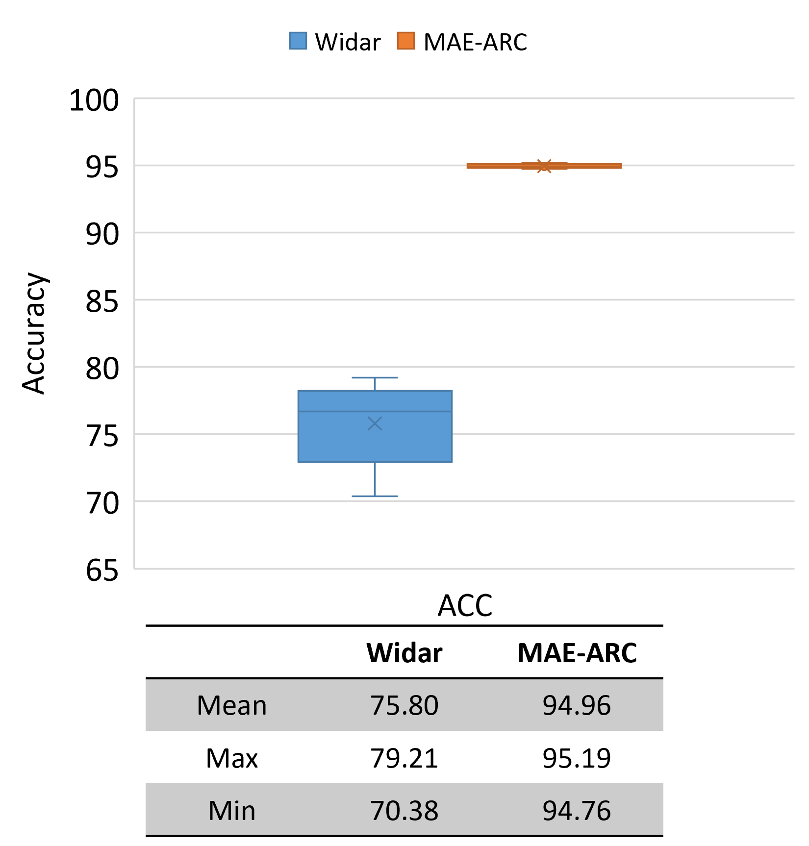
(a) Accuracy Comparison

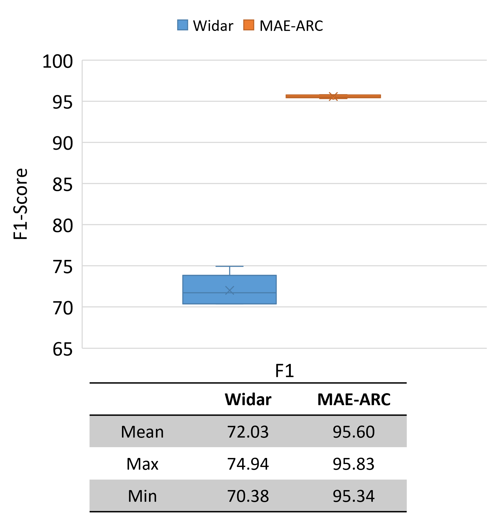
(b) F1-Score Comparison

Figure 4: Performance comparison between Widar and MAE-ARC.

Method	Processing Time (second per sample)	Parameters (Mb)
MAE-ARC	0.00797	42.89
Widar	164.906	0.5627

Table 3: Processing Speed and Number of Parameters of MAE-ARC and WiDAR

4.5 Impact of Hyperparamenter Alpha

In Algorithm 2, specifically for MAE-ARC, we introduced a hyperparameter called alpha to manage the influence of both the MSE loss and ARC loss (cosine similarity) on the model’s performance throughout the learning process. In order to study the impact of alpha, in Figure 5(a) and 5(b) we show the impact of alpha to MAE-ARC’s accuracy and F1-score on Widar3.0.

From the analysis of the two figures, it’s evident that the performance of the MAE-ARC model generally declines as alpha increases, and this effect is more pronounced in the case of the single-layer perceptron. Among the alpha values we experimented with, the best model performance was achieved when alpha was set to 0.1. This trend can be attributed to the fact that, for MAE-ARC, the MSE loss corresponds to the uniformity objective, while the ARC loss corresponds to the alignment objective. When alpha becomes excessively large, the alignment objective dominates. This results in the model’s tendency to map all samples to a single point in the feature space, essentially leading to a collapsed solution.

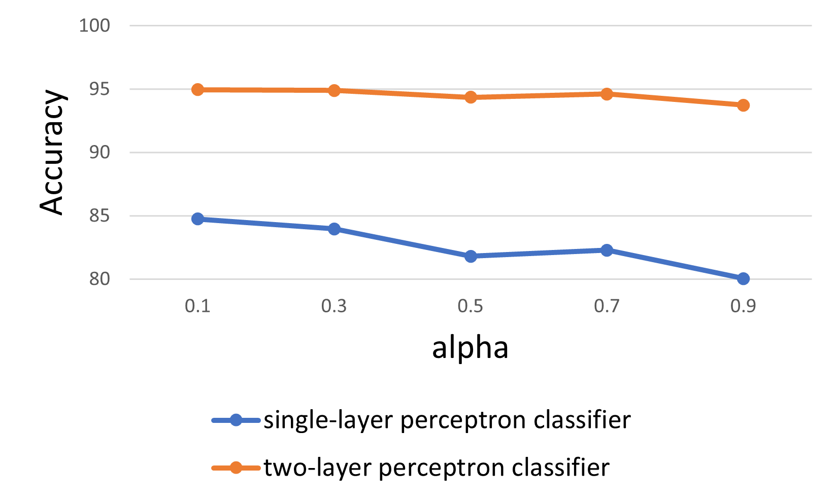
(a) Impact to accuracy

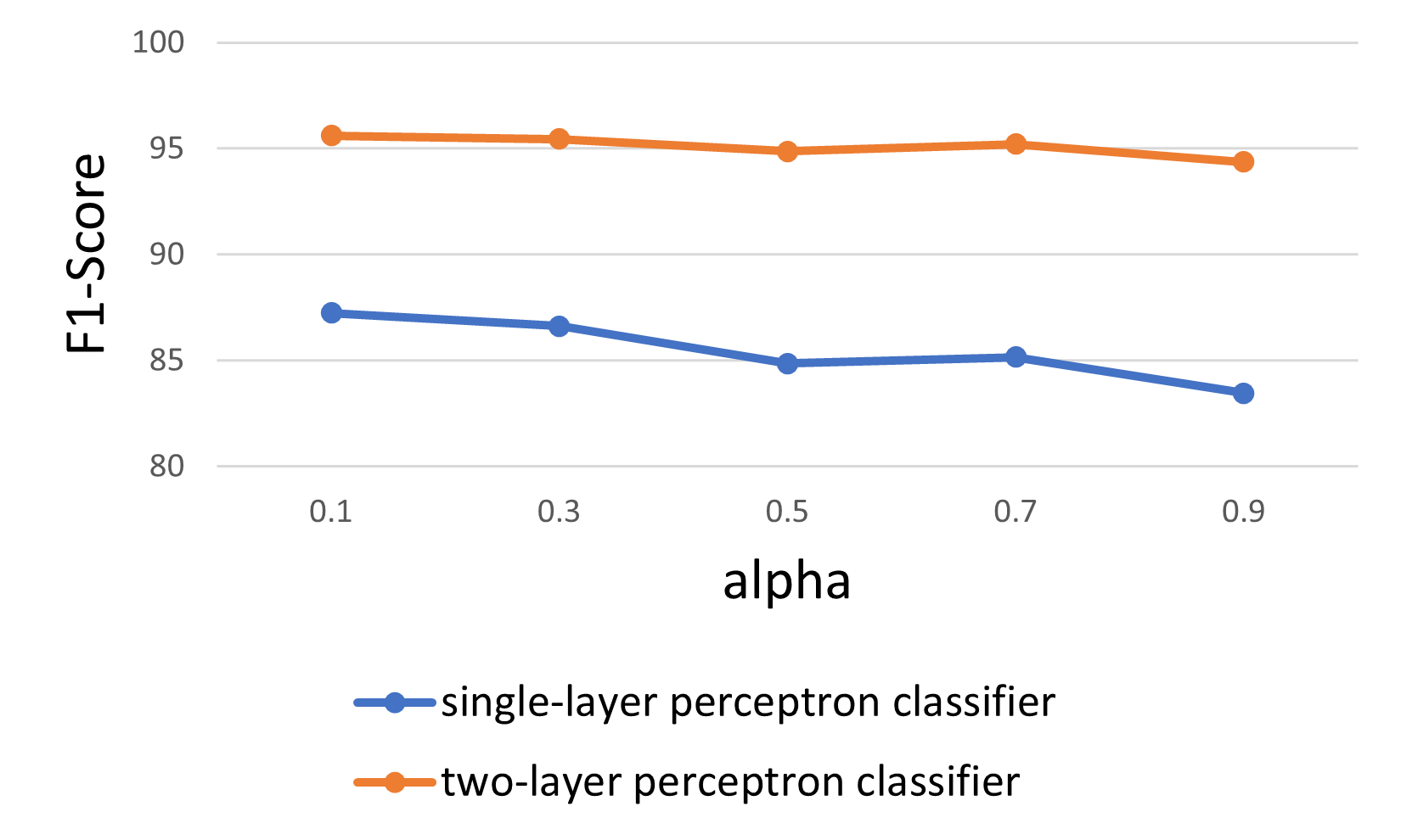
(b) Impact to F1-score

Figure 5: Impact of alpha to MAE-ARC’s accuracy and F1-score on Widar3.0.

4.6 Impact of Conjugate Multiplication

To validate our analysis regarding the influence of phase noise on ARC in Section 3.2, we conducted experiments to assess the model’s performance using phase (Angle) and phase after conjugated multiplication (ConjAngle). All results are shown in Figures 6(a) to 6(d). Figures 6(a) and 6(b) depict the influence of the conjugate multiplication step on the performance of the ARC strategy for MOCO and MAE when utilizing a single-layer perceptron as the classifier. Figures 6(c) and 6(d) showcase the effect of the conjugate multiplication step on the performance of the ARC strategy for MOCO and MAE when employing a two-layer perceptron as the classifier.

Evidently, the ARC strategy results in a degradation in model performance when employing the "Angle" feature in all scenarios. Conversely, except for Figure 6(a), the ARC strategy enhances model performance in all "ConjAng" cases. As previously analyzed, we attribute this phenomenon to the presence of a phase offset, which causes the ARC strategy to guide the model in learning the phase offset pattern rather than the action pattern. With the application of conjugate multiplication, the phase offset term is eliminated, allowing the model to correctly learn the action pattern.

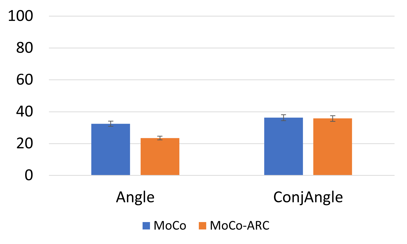
(a) The accuracy of MOCO and MOCO-ARC when using a single-layer perceptron.

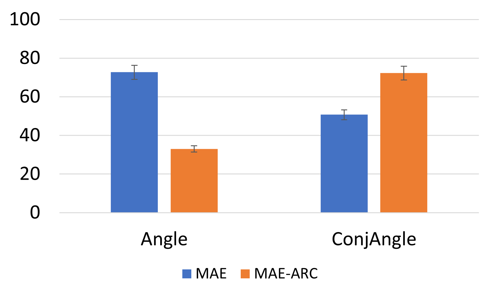
(b) The accuracy of MAE and MAE-ARC when using a single-layer perceptron.

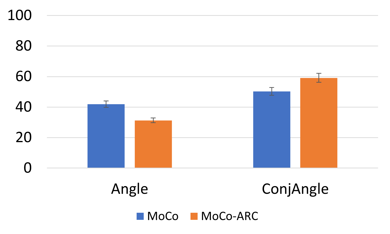
(c) The accuracy of MOCO and MOCO-ARC when using a two-layer perceptron.

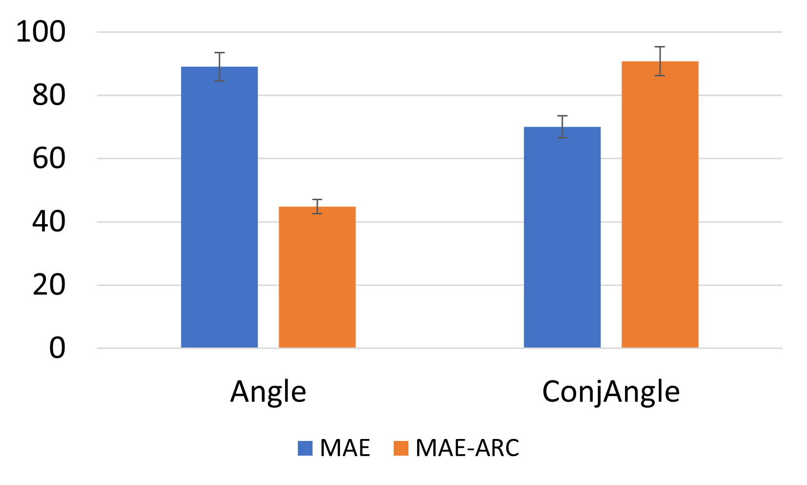
(d) The accuracy of MAE and MAE-ARC when using a two-layer perceptron.

Figure 6: Impact of Conjugate Multiplication.

5 Conclusion

In this paper, we highlight a critical observation: the direct application of SSL (Self-Supervised Learning) algorithms, particularly contrastive learning, originally designed for different domains like computer vision, does not yield the expected performance when applied to Channel State Information (CSI) data, as discussed in [2]. We attribute this phenomenon to the mismatch between the alignment criteria designed for the original data modalities and the nature of CSI data.

To tackle these challenges, we introduce ARC, a novel strategy aimed at defining alignment criteria for feature spaces tailored specifically to CSI data. We provide a theoretical analysis from the perspective of CSI data structure, explaining how ARC promotes feature space alignment while preserving semantic consistency. Our approach is validated through an extensive series of experiments, offering empirical proof of its effectiveness. ARC is easy to integrate into existing algorithms with minimal code modifications. Our goal is for ARC to facilitate the adoption of SSL techniques within the CSI domain, potentially surpassing the performance benchmarks established by supervised learning, much like the success of SSL in the computer vision domain.

In our future work, we will delve into the possibility of integrating ARC into other categories of SSL algorithms, including relationship-prediction-based SSL methods. Furthermore, we aim to investigate whether ARC can offer benefits to related algorithms addressing the domain adaptation problem, an area of increasing interest within the CSI domain.

References

- [1] Yi Zhang, Yue Zheng, Kun Qian, Guidong Zhang, Yunhao Liu, Chenshu Wu, and Zheng Yang. Widar3. 0: Zero-effort cross-domain gesture recognition with wi-fi. IEEE Transactions on Pattern Analysis and Machine Intelligence, 44(11):8671–8688, 2021.
- [2] Ke Xu, Jiangtao Wang, Hongyuan Zhu, and Dingchang Zheng. Self-supervised learning for wifi csi-based human activity recognition: A systematic study. arXiv preprint arXiv:2308.02412, 2023.
- [3] Kaiming He, Haoqi Fan, Yuxin Wu, Saining Xie, and Ross Girshick. Momentum contrast for unsupervised visual representation learning. In Proceedings of the IEEE/CVF conference on computer vision and pattern recognition, pages 9729–9738, 2020.
- [4] Tongzhou Wang and Phillip Isola. Understanding contrastive representation learning through alignment and uniformity on the hypersphere. In International Conference on Machine Learning, pages 9929–9939. PMLR, 2020.
- [5] Yongsen Ma, Gang Zhou, and Shuangquan Wang. Wifi sensing with channel state information: A survey. ACM Computing Surveys (CSUR), 52(3):1–36, 2019.
- [6] Ju Wang, Jie Xiong, Hongbo Jiang, Kyle Jamieson, Xiaojiang Chen, Dingyi Fang, and Chen Wang. Low human-effort, device-free localization with fine-grained subcarrier information. IEEE Transactions on Mobile Computing, 17(11):2550–2563, 2018.
- [7] Kaiming He, Xinlei Chen, Saining Xie, Yanghao Li, Piotr Dollár, and Ross Girshick. Masked autoencoders are scalable vision learners. In Proceedings of the IEEE/CVF conference on computer vision and pattern recognition, pages 16000–16009, 2022.
- [8] Zhenda Xie, Zheng Zhang, Yue Cao, Yutong Lin, Jianmin Bao, Zhuliang Yao, Qi Dai, and Han Hu. Simmim: A simple framework for masked image modeling. In Proceedings of the IEEE/CVF Conference on Computer Vision and Pattern Recognition, pages 9653–9663, 2022.
- [9] Dan Wu, Daqing Zhang, Chenren Xu, Yasha Wang, and Hao Wang. Widir: Walking direction estimation using wireless signals. In Proceedings of the 2016 ACM international joint conference on pervasive and ubiquitous computing, pages 351–362, 2016.
- [10] Daqing Zhang, Hao Wang, and Dan Wu. Toward centimeter-scale human activity sensing with wi-fi signals. Computer, 50(1):48–57, 2017.
- [11] Youwei Zeng, Dan Wu, Jie Xiong, Jinyi Liu, Zhaopeng Liu, and Daqing Zhang. Multisense: Enabling multi-person respiration sensing with commodity wifi. Proceedings of the ACM on Interactive, Mobile, Wearable and Ubiquitous Technologies, 4(3):1–29, 2020.
- [12] Jinyi Liu, Wenwei Li, Tao Gu, Ruiyang Gao, Bin Chen, Fusang Zhang, Dan Wu, and Daqing Zhang. Towards a dynamic fresnel zone model to wifi-based human activity recognition. Proceedings of the ACM on Interactive, Mobile, Wearable and Ubiquitous Technologies, 7(2):1–24, 2023.
- [13] Qifan Pu, Sidhant Gupta, Shyamnath Gollakota, and Shwetak Patel. Whole-home gesture recognition using wireless signals. In Proceedings of the 19th annual international conference on Mobile computing & networking, pages 27–38, 2013.
- [14] Kun Qian, Chenshu Wu, Zheng Yang, Yunhao Liu, and Kyle Jamieson. Widar: Decimeter-level passive tracking via velocity monitoring with commodity wi-fi. In Proceedings of the 18th ACM International Symposium on Mobile Ad Hoc Networking and Computing, pages 1–10, 2017.
- [15] Xiang Li, Daqing Zhang, Qin Lv, Jie Xiong, Shengjie Li, Yue Zhang, and Hong Mei. Indotrack: Device-free indoor human tracking with commodity wi-fi. Proceedings of the ACM on Interactive, Mobile, Wearable and Ubiquitous Technologies, 1(3):1–22, 2017.
- [16] Kun Qian, Chenshu Wu, Yi Zhang, Guidong Zhang, Zheng Yang, and Yunhao Liu. Widar2. 0: Passive human tracking with a single wi-fi link. In Proceedings of the 16th annual international conference on mobile systems, applications, and services, pages 350–361, 2018.
- [17] Ting Chen, Simon Kornblith, Mohammad Norouzi, and Geoffrey Hinton. A simple framework for contrastive learning of visual representations. In International conference on machine learning, pages 1597–1607. PMLR, 2020.
- [18] Mathilde Caron, Ishan Misra, Julien Mairal, Priya Goyal, Piotr Bojanowski, and Armand Joulin. Unsupervised learning of visual features by contrasting cluster assignments. Advances in neural information processing systems, 33:9912–9924, 2020.
- [19] Carl Doersch, Abhinav Gupta, and Alexei A Efros. Unsupervised visual representation learning by context prediction. In Proceedings of the IEEE international conference on computer vision, pages 1422–1430, 2015.
- [20] Spyros Gidaris, Praveer Singh, and Nikos Komodakis. Unsupervised representation learning by predicting image rotations. arXiv preprint arXiv:1803.07728, 2018.
- [21] Aaqib Saeed, Flora D Salim, Tanir Ozcelebi, and Johan Lukkien. Federated self-supervised learning of multisensor representations for embedded intelligence. IEEE Internet of Things Journal, 8(2):1030–1040, 2020.
- [22] Dongxin Liu, Tianshi Wang, Shengzhong Liu, Ruijie Wang, Shuochao Yao, and Tarek Abdelzaher. Contrastive self-supervised representation learning for sensing signals from the time-frequency perspective. In 2021 International Conference on Computer Communications and Networks (ICCCN), pages 1–10. IEEE, 2021.
- [23] Aaqib Saeed, Victor Ungureanu, and Beat Gfeller. Sense and learn: Self-supervision for omnipresent sensors. Machine Learning with Applications, 6:100152, 2021.
- [24] Zhihan Yue, Yujing Wang, Juanyong Duan, Tianmeng Yang, Congrui Huang, Yunhai Tong, and Bixiong Xu. Ts2vec: Towards universal representation of time series. In Proceedings of the AAAI Conference on Artificial Intelligence, volume 36, pages 8980–8987, 2022.
- [25] Wei Wang, Alex X Liu, Muhammad Shahzad, Kang Ling, and Sanglu Lu. Understanding and modeling of wifi signal based human activity recognition. In Proceedings of the 21st annual international conference on mobile computing and networking, pages 65–76, 2015.
- [26] Daniel Halperin, Wenjun Hu, Anmol Sheth, and David Wetherall. Tool release: Gathering 802.11n traces with channel state information. ACM SIGCOMM CCR, 41(1):53, Jan. 2011.