Calibrating approximate Bayesian credible intervals of gravitational-wave parameters

Abstract

Approximations are commonly employed in realistic applications of scientific Bayesian inference, often due to convenience if not necessity. In the field of gravitational-wave (GW) data analysis, fast-to-evaluate but approximate waveform models of astrophysical GW signals are sometimes used in lieu of more accurate models to infer properties of a true GW signal buried within detector noise. In addition, a Fisher-information-based normal approximation to the posterior distribution can also be used to conduct inference in bulk, without the need for extensive numerical calculations such as Markov chain Monte Carlo (MCMC) simulations. Such approximations can generally lead to an inaccurate posterior distribution with poor statistical coverage of the true posterior. In this article, we present a novel calibration procedure that calibrates the credible sets for a family of approximate posterior distributions, to ensure coverage of the true posterior at a level specified by the analyst. Tools such as autoencoders and artificial neural networks are used within our calibration model to compress the data (for efficiency) and to perform tasks such as logistic regression. As a proof of principle, we demonstrate our formalism on the GW signal from a high-mass binary black hole merger, a promising source for the near-future space-based GW observatory LISA.

I Introduction

The ground-breaking observation of a gravitational-wave (GW) signal spectacularly opened the field of gravitational-wave astronomy on the 14th of September, 2015. The ground-based gravitational-wave observatories, the Laser Interferometer Gravitational-Wave Observatory (LIGO) in Livingston and Hanford, observed a GW signal emanating from the coalescence of two stellar-mass black holes (BHs)  abbott2016observation . This feat was achieved through the use of sophisticated statistical signal processing algorithms and accurate waveform templates used to filter the data stream veitch2015parameter ; abbott2020guide ; abbott2016gw150914 . In a traditional (ground-based) matched-filtering search, template banks are used to detect the presence of a signal buried within the instrumental noise kumar2014template ; usman2016pycbc ; ajith2014effectual ; adams2016low . Once a candidate signal in the data stream is established, stochastic sampling algorithms, such as Markov chain Monte Carlo (MCMC), are used to estimate of the parameter set that best describes the corresponding astrophysical source  christensen2022parameter ; meyer2022computational ; finn1992detection . To do this both efficiently and accurately, we require astrophysical waveform models to be both cheap to generate and sufficiently detailed to describe the fully-relativistic waveform in the data stream Miller2005 .

The current state-of-the-art waveform modelling technique for binary black holes with mass ratios $\lesssim 20$ is numerical relativity (NR), where the fully general Einstein equations are numerically solved for the space-time metric perturbations lehner2014numerical ; pretorius2005numerical ; lehner2001numerical ; boyle2019sxs . These NR simulations are the most accurate method to date we have to generate comparable mass BHs, but can take months to generate a small number of orbits lousto2011orbital ; blackman2015fast . For data analysis, which relies on generating hundreds of thousands of waveforms with multiple cycles, this is computationally infeasible. In order to circumvent this, various waveform approximations have been developed that rely on a hybrid between the Post-Newtonian (PN) formalism and NR buonanno1999effective ; nagar2019efficient ; cotesta2020frequency ; khan2016frequency ; husa2016frequency ; Pratten_2020 . This has the major advantage that these waveform models are faster to generate, but with the cost that they are not truly faithful to the GW signal hidden within the data stream. Modelling errors can result in an overall reduced sensitivity in the detection of actual signals. Using non-faithful waveforms can also impact inference: we may potentially recover biased parameter estimates, and/or claim incorrectly how precise we can measure the parameters in question Flanagan:1997kp ; Miller2005 ; Cutler:2007mi . Additionally, it can be shown that biases arising from approximate waveform models scale inversely in the limit of high signal-to-noise ratio (SNR) Cutler:2007mi . Further, waveform inaccuracies could result in systematic errors in parameter estimates and even dominate them, especially with multiple overlapping signals Hu_2023 ; antonelli2021noisy ; pizzati2022toward ; hu2023accumulating .

In our work, we will restrict our attention to a particular class of sources expected to be observed by the space-based gravitational-wave observatory: the Laser Interferometer Space Antenna (LISA) lisa:2017 ; baker2019laser . In contrast to ground-based detectors, which are limited by seismic noise at lower frequencies, the LISA instrument will achieve optimum sensitivity in the mHz GW frequency band, providing the means to probe the rich structure of high mass binaries. One of the most promising sources of mHz gravitational radiation will be the collisions of comparable massive black hole binaries (MBHBs) with masses of $10^{5}-10^{7}M_{\odot}$ up to redshifts of $z\lesssim 20$. Observation of these MBHBs at specific redshifts gives one a means to probe various formation channels for MBHBs  berti2006gravitational ; hughes2002untangling ; sesana2005gravitational ; vecchio2004lisa . Unlike sources observed by ground-based detectors, MBHBs will be extremely loud, with SNRs up to $\sim 1000$, offering strong constraints on the parameters that govern the signal cornish2007search ; porter2008effect . Due to the strength of these signals and the precision in which we can measure their parameters, they will provide powerful tests of general relativity (GR) yagi2016black ; barausse2020prospects ; gair2013testing .

With the immense strength of these signals, we will require exceptionally accurate waveform models to ensure that recovered parameters are not biased and that uncertainties are correctly quantified. For this reason, calibration techniques that provide a means to “correct” inference resulting from an approximate waveform model to an exact waveform model (such as a NR simulation) may be viewed as essential. An early example of this was presented in Flanagan:1997kp ; Miller2005 ; Cutler:2007mi , which showed how to estimate the bias (and thus the accurate maximum a posteriori estimate) in the linear-signal regime. More recently, Gaussian process regression has been developed as a viable method for interpolating and marginalising over model error in the GW likelihood, thus calibrating the likelihood itself before it is used for posterior estimation Moore:2014pda ; Moore:2015sza ; Chua:2019wgs ; Liu:2023oxw . Similar studies can also be found with ground-based detectors, like LIGO and Virgo, as well as preparations for Cosmic Explorer and Einstein Telescope. Early Fisher studies, with an approximation to the full likelihood, may not be applicable for low SNR events. Full analyses into the full parameter space were needed when correcting the model uncertainties. Signal-specific calibration with marginalization in gravitational-wave inference was implemented read2023waveform . The application of the Bayesian method was also proposed to marginalize the ignorance of (unknown) higher PN order terms and give general directive calibrations PhysRevD.108.044018 .

When the generative model lacks computational efficiency for executing the MCMC simulation, resorting to posterior density approximation becomes an appealing option and the MCMC simulation can be avoided. This is often seen in Bayesian inference and some well-known approximations include the mean field approximation in the Variational Bayes jordan:1999 and Laplace approximation Mackay:1998 ; Walker:1969 . In this paper, the posterior density is normally approximated by imposing the Fisher matrix approach to the likelihood and the uniform prior. The Fisher matrix for the GW likelihood can be expressed in terms of waveform derivatives of the approximate model (which may need to be computed numerically, but using far fewer evaluations of the model than posterior sampling). It is widely used throughout GW astronomy to cheaply forecast precision statements on parameters vallisneri2008use and to predict biases on parameter estimates through the use of non-faithful waveform models Cutler:2007mi . As the Fisher matrix lends itself to calculations in bulk, it is often also used to approximate and hence study a family of posteriors over a space of GW signals Klein_2016 ; babak2017science ; berry2019unique ; colpi2019gravitational . Thus there is plenty of motivation for methods that can calibrate the family of approximate normal posteriors obtained via the Fisher matrix.

In this paper, we introduce a novel calibration technique that approaches the problem from another angle, using the formalism presented by lee:2019 . In the Bayesian framework, the uncertainty about unknowns is probabilistically represented by the posterior distribution. When an approximate waveform generation model is used or a likelihood/posterior is approximated, the resulting inference is not exact. Operational coverage of a credible set of a parameter vector based on an approximate posterior measures how much of the exact posterior probability mass lies in this set and, it can be interpreted as an error estimate for the approximate posterior. A practical operational coverage estimator allows us to estimate an error of posterior approximation for any observed waveform generated from a prior distribution (lee:2019, ; xing:2019, ). To perform the calibration formalism, it is necessary to generate a large number of posteriors using an approximate waveform model. This would clearly become computationally prohibitive with expensive posterior simulation methods. Due to the usage of normal approximations via a Fisher-based formalism to the posteriors, expensive posterior simulation is not required and, the practical operational coverage estimator is acquired with a more budget-friendly computing cost.

Here, we present a practical estimator for gravitational-wave data analysis and demonstrate how to compute the calibrated credible set of an approximate posterior that corresponds to the desired exact posterior probability mass. Systematic studies usually focus on correcting a single posterior, generated via an approximate waveform model at a specific point in parameter space antonelli2021noisy . Instead, we propose a method that, after a training scheme (on the prior space of samples), near-instantaneous calibrated posterior estimates can be generated over the entire signal space. In other words, we devise a scheme that can calibrate a family of posteriors, rather than a single one.

This paper is organised as follows. In Section II we set notations and introduce the data analysis concepts that will be used throughout this work. In Section III, we summarise the work of lee:2019 , outlining a framework that can be used to calibrate the statistical coverage of approximate posterior distributions to the exact posterior distribution as if parameter estimation was performed using a more faithful waveform model. In Section IV we demonstrate this calibration procedure using a simple toy example and finally show its general applicability on an MBHB source within the LISA framework in Section V. Our conclusions and scope for future work is presented in section VI.

II Gravitational-wave data analysis

II.1 Noise modelling and likelihood

The typical time-domain data stream observed by the LISA instrument will be a combination of TDI variables $X=\{A,E,T\}$, representing the response of the LISA instrument to the plus and cross polarisations of the incoming GW source in the transverse-traceless gauge tinto:2021 ; tinto:2023 :

$$d_{o}^{(X)}(t)=h_{\text{e}}^{(X)}(t;\boldsymbol{\theta}_{\text{0}})+n^{(X)}(t),\quad X=\{A,E,T\}.$$ (1)

Here $d_{o}$ is the observed data stream, $\boldsymbol{\theta}_{0}$ are the true parameters of the true gravitational wave $h^{(X)}_{\text{e}}$, and $n^{(X)}(t)$ are noise fluctuations arising from perturbations to the LISA instrument from unresolvable GW sources and non-GW instrumental perturbations. In our work, we will perform inference on a single waveform within the data streams $d^{(X)}$ and ignore potential multiple signals within the data stream, such as would be considered in the global fit littenberg:2023 . We make the assumption that the noise $n^{(X)}$ in each channel is a weakly stationary Gaussian stochastic process with zero mean, coloured by the power spectral density (PSD) of their respected TDI channel. A consequence of this is that the noise $n^{(X)}$ is uncorrelated in the frequency domain, resulting in a purely diagonal noise covariance matrix $\Sigma$  wiener1930generalized ; khintchine1934korrelationstheorie ; burke2021extreme :

$$\Sigma(f,f^{\prime}) =\langle\hat{n}^{(X)}(f)(\hat{n}^{(X)}(f^{\prime}))^{\star}\rangle$$ (2)

$$=\frac{1}{2}\delta(f-f^{\prime})S^{(X)}_{n}(f^{\prime})\,.$$ (3)

for $f\in(0,\infty)$. Here $\langle\cdot\rangle$ denotes an average ensemble over many noise realisations, $\delta$ is the Dirac delta function and $S_{n}^{(X)}$ is the power spectral density (PSD) of the noise process within a channel $X$. Hatted quantities refer to the Fourier transform with convention,

$$\hat{h}(f)=\int_{0}^{\infty}\text{d}t\,h(t)\exp(-2\pi\text{i}ft).$$ (4)

Assuming that the arm-lengths of the LISA interferometer are both equal and constant, it can be shown that the noise across channels $X$ is independent and thus uncorrelated tinto:2021 ; tinto:2023 . From equation (3), Whittle showed that the likelihood in the frequency domain takes the form whittle:1957

$$p(n)=-\frac{1}{2}\sum_{X}(n|n)^{(X)}$$ (5)

with inner product finn1992detection ; Flanagan:1997kp

$$(a|b)^{(X)}=4\text{Re}\int_{0}^{\infty}\text{d}f\frac{\hat{a}^{(X)}(f)(\hat{b}^{(X)}(f^{\prime}))^{\star}}{S^{(X)}_{n}(f^{\prime})}.$$ (6)

Substituting equation (1) into (5), we obtain the usual likelihood used throughout gravitational-wave astronomy finn1992detection ; meyer2022computational ; burke2021extreme

$$p(d|\boldsymbol{\theta})=-\frac{1}{2}\sum_{X}(d-h_{\text{m}}|d-h_{\text{m}})^{(X)},$$ (7)

where $h_{\text{m}}$ are our approximate model templates, favourably quick to generate and used when inferring parameters $\boldsymbol{\theta}$.

The signal-to-noise ratio (SNR), $\rho$, is a quantity used to determine the power of the signal when compared to noise. Within the framework of matched filtering woodward2014probability ; turin1960introduction , the optimal matched filtering SNR takes the form finn1992detection

$$\rho_{X}^{2}=(h_{m}|h_{m})^{(X)}=4\int_{0}^{\infty}\text{d}f\frac{|\hat{h}(f)|^{2}}{S^{(X)}_{n}(f)},$$ (8)

with total (squared) SNR across $X=\{A,E,T\}$ given by summing equation (8) in quadrature $\rho^{2}=\sum_{X}(h_{\text{m}}|h_{\text{m}})^{(X)}$.

We now describe how we generate detector noise given that the noise is both stationary and we know, a-priori, the PSD of the noise process $n^{(X)}$.

The frequency domain equation (3) can be discretized in the continuum limit to give the covariance of the noise between two frequency bins $f_{i}$ and $f_{j}$:

$$\hat{\Sigma}_{ij} = \mathbb{E}_{d}[\hat{n}^{(X)}(f_{i})(\hat{n}^{(X)}(f_{j}))^{\star}]$$ (9)

$$= S_{n}^{(X)}(f_{i})\delta_{ij}/2\Delta f.$$ (10)

Here $f_{i}\in[0,\Delta f,\ldots,(\frac{N}{2})\Delta f]$ is an individual frequency bin, $\Delta f=1/N\Delta t=1/T_{\text{obs}}$ the spacing between frequency bins, $N$ the length of the time series and $\Delta t$ the sampling interval.

Equation (10) highlights that, for stationary Gaussian noise, the frequency bins for $i\neq j$ are uncorrelated. Focusing on the diagonal elements of (10), it is possible to show that the real and imaginary components of the noise follows a Gaussian distribution:

$$\text{Re}(\hat{n}^{(X)}(f_{i}) =N\left(0,\frac{S_{n}^{(X)}(f_{i})}{4\Delta f}\right)$$ (11a)

$$\text{Im}(\hat{n}^{(X)}(f_{i}) =N\left(0,\frac{S_{n}^{(X)}(f_{i})}{4\Delta f}\right)\,.$$ (11b)

To simulate noise, we thus draw components of the noise from equations (11a) and (11b) given PSDs $S_{n}^{(X)}$ for each of the channels $X=\{A,E,T\}$. An exact signal is then generated, added to this specific noise realisation, and this constructs the data set $d^{(X)}(t)$ in (1).

As will be discussed in II.2, assuming that the likelihood is consistent with the noise model, the detector noise will encode a statistical fluctuation forcing a deviation between the recovered and true parameters. In reality, the recovered parameters will not be centred on the true parameters due to the presence of two features: waveform modelling errors and noise. The next section describes how one can compute the bias on parameters due to waveform modelling errors and statistical fluctuations due to the inclusion of noise.

II.2 Fisher matrix

In our work we will use a Fisher matrix formalism to generate approximate distributions on parameters given an observed data stream $p(\boldsymbol{\theta}|d_{o})$ finn1992detection ; vallisneri2008use . In the high SNR limit, it is expected that the distribution of parameter sets is a multivariate Gaussian defined by a mean vector and covariance matrix. Here we will show how one can approximate both the mean vector and covariance matrix using a Fisher matrix approach, rather than using costly MCMC simulations. Here we generalise the results from Flanagan:1997kp ; Miller2005 ; Cutler:2007mi to account for the three LISA channels $A,E$ and T.

We denote the best fit parameter $\theta^{i}_{\text{bf}}$ as the maximum likelihood estimate (MLE) that maximises equation (7)

$$\sum_{X=\{A,E,T\}}(\partial_{i}h^{(X)}_{m}(t;\boldsymbol{\theta}_{\text{bf}})|d^{(X)}-h^{(X)}_{m}(t;\boldsymbol{\theta}_{\text{bf}}))=0\,.$$ (12)

Here $\partial_{i}:=\partial/\partial\theta^{i}$ denotes a partial derivative with respect to $\theta^{i}$. Now consider a small perturbation around the true parameters $\boldsymbol{\theta}_{\text{bf}}=\boldsymbol{\theta}_{0}+\Delta\boldsymbol{\theta}$ for $\Delta\boldsymbol{\theta}=(\boldsymbol{\theta}_{\text{bf}}-\boldsymbol{\theta}_{0})$. By applying the linear signal approximation, an expansion in $\Delta\boldsymbol{\theta}\ll 1$ to first order in our model templates gives

$$h^{(X)}_{m}(\boldsymbol{\theta}_{0})\approx h^{(X)}_{m}(\boldsymbol{\theta}_{\text{bf}})-\partial_{i}h^{(X)}_{m}(\boldsymbol{\theta}_{\text{bf}})\Delta\theta^{i}\,,$$ (13)

From this point onward, we will drop the (fixed) time coordinate $t$ for notational convenience. Equation (13) can then be used in the expression $d^{(X)}-h^{(X)}_{m}$ to find

$$d^{(X)}-h^{(X)}_{m}(\boldsymbol{\theta}_{\text{bf}}) =n^{(X)}+h^{(X)}_{e}(\boldsymbol{\theta}_{0})-h^{(X)}_{m}(\boldsymbol{\theta}_{\text{bf}})$$

$$=n^{(X)}+h^{(X)}_{e}(\boldsymbol{\theta}_{0})-h^{(X)}_{m}(\boldsymbol{\theta}_{0})+h^{(X)}_{m}(\boldsymbol{\theta}_{\text{0}})-h^{(X)}_{m}(\boldsymbol{\theta}_{\text{bf}})$$

$$\approx n^{(X)}+\delta h^{(X)}(\boldsymbol{\theta}_{0})-\partial_{i}h^{(X)}_{m}(\boldsymbol{\theta}_{\text{bf}})\Delta\theta^{i}+(\Delta\theta^{i})^{2}$$ (14)

for $\delta h^{(X)}(\boldsymbol{\theta}_{0})=h_{e}^{(X)}(\boldsymbol{\theta}_{0})-h_{m}^{(X)}(\boldsymbol{\theta}_{0})$ denoting residuals between the true waveform $h_{e}^{(X)}$ and the approximate waveform $h_{m}^{(X)}$. When there are no mismodelling errors present, the term $\delta h^{(X)}=0$. Substituting equation (14) into (12), one obtains at first order in $\Delta\theta^{i}$

$$\sum_{X=\{A,E,T\}}[\Delta\theta^{j}(\partial_{j}h_{m}(\boldsymbol{\theta}_{\text{bf}})|\partial_{i}h_{m}(\boldsymbol{\theta}_{\text{bf}}))^{(X)}-(\partial_{j}h_{m}(\boldsymbol{\theta}_{\text{bf}})|n)^{(X)}-(\partial_{j}h_{m}(\boldsymbol{\theta}_{\text{bf}})|\delta h(\boldsymbol{\theta}_{\text{0}}))^{(X)}]=0$$ (15)

Defining the matrix

$$(\Gamma_{AET})_{ij}=\sum_{X=\{A,E,T\}}(\partial_{i}h_{m}(\boldsymbol{\theta}_{\text{bf}})|\partial_{j}h_{m}(\boldsymbol{\theta}_{\text{bf}}))^{(X)}$$ (16)

it is then possible to invert the matrix-vector equation (15) to calculate $\Delta\theta^{i}$

$$\Delta\theta^{i}=(\Gamma_{AET}^{-1})^{ij}\left[\sum_{X}(\partial_{j}h_{m}(\boldsymbol{\theta}_{\text{bf}})|n)^{(X)}+(\partial_{j}h_{m}(\boldsymbol{\theta}_{\text{bf}})|\delta h(\boldsymbol{\theta}_{\text{0}}))^{(X)}\right].$$ (17)

In the presence of noise fluctuations $n^{(X)}$ and waveform modelling errors $h_{e}\neq h_{m}$, there are two sources of discrepancy between the recovered parameters $\theta^{i}_{\text{bf}}$ and true parameters $\theta^{i}_{0}$ described by equation (17). Each of these terms represent a statistical error, determined by the presence of noise and the second a systematic error, a consequence of non-faithful model templates $h_{m}$

$$\Delta\theta^{i}_{n} =(\Gamma^{-1}_{AET})^{ij}\sum_{X}(\partial_{j}h_{\text{m}}(\boldsymbol{\theta}_{\text{bf}})|n)^{(X)},$$ (18)

$$\Delta\theta^{i}_{\text{sys}} =(\Gamma^{-1}_{AET})^{ij}\sum_{X}(\partial_{j}h_{\text{m}}(\boldsymbol{\theta}_{\text{bf}})|\delta h(\boldsymbol{\theta}_{0}))^{(X)}.$$ (19)

The first term (18) enforces a statistical fluctuation to the recovered parameters. Since the noise has mean zero, the statistic $\theta^{i}_{\text{n,bf}}=\theta^{i}_{0}+(\widehat{\Delta\theta^{i}_{n}})_{AET}$ is an unbiased estimator of the true parameters such that $\mathbb{E}[\theta^{i}_{\text{n,bf}}]=\theta^{i}_{0}$. The quantity (19) governs the bias in the recovered parameters due to using inaccurate waveform models where $\delta h^{(X)}(\boldsymbol{\theta}_{0})\neq 0$. The overall bias is thus given by the second term in equation (19)

$$\mathbb{E}[\theta^{i}_{\text{bf}}]=\theta_{0}^{i}+(\Gamma^{-1}_{AET})^{ij}\sum_{X}(\partial_{j}h_{\text{m}}(\boldsymbol{\theta}_{\text{bf}})|\delta h(\boldsymbol{\theta}_{0})^{(X)}).$$ (20)

Note that since $h\sim\rho$ and $S_{n}(f)\sim\rho^{0}$, we have that $\Gamma^{-1}\sim\rho^{-2}$ giving the scaling relationship for the statistical uncertainty $(\widehat{\Delta\theta^{i}_{n}})_{AET}\sim O(1/\rho)$. Similarly, for the systematic error, the scaling relationship is given by $(\widehat{\Delta\theta^{i}_{\text{sys}}})_{AET}\sim O(\rho^{0})$ and is thus independent of the SNR of the source. Therefore, if the signal-to-noise ratio of the underlying signal is large, then the (relative) magnitude of the systematic error will be larger when compared to the statistical fluctuation. Further details can be found in Flanagan:1997kp ; Miller2005 ; Cutler:2007mi ; antonelli2021noisy .

In the limit of small waveform modelling errors $|\delta h^{(X)}|^{2}\ll\rho^{0}$ and high SNR, the Fisher matrix yields an approximation to the predicted covariance matrix of the posterior distribution

$$\mathbb{E}[(\Delta\theta^{i}_{\text{bf}})(\Delta\theta_{\text{bf}}^{j})]\approx(\Gamma_{AET}^{-1})^{ij}\,.$$ (21)

with rooted diagonal elements an approximation to how well one can constrain the parameters of the system. The Fisher matrix is widely used within gravitational-wave astronomy to cheaply compute precision measurements on parameters of interest. Precision measurements are given by the rooted diagonals of the inverse of the Fisher matrix

$$\Delta\theta^{i}_{\text{stat}}=\sqrt{(\Gamma^{-1})^{ii}}\quad\text{no sum.}$$ (22)

where $\Delta\theta^{i}_{\text{stat}}$ is the statistical error, the $1\sigma$ deviation (through expectation) in the recovered parameters due to noise fluctuations. For systematic studies in Cutler-Valisneri framework Cutler:2007mi , the ratio between (19) and (22) is computed. If the bias on parameters exceed the statistical uncertainty, then the proposed waveform model is not suitable for parameter estimation.

In our work, we will not focus on error induced due to approximate waveform models. Instead, we will focus on the notion of coverage given by an approximate posterior distribution. The “coverage” of a posterior density describes the probability that the true parameters are contained within the posteriors credible set. The Cutler Valisneri formalism can be discussed in terms of coverage of a posterior: If the (assumed normal) approximate posterior has a 68% coverage, then the waveform model will be deemed suitable for parameter estimation. The primary focus of our work is to calibrate the coverage of an approximate posterior to a much higher level, specified by the user. The final (calibrated) credible region will then contain the true parameters with higher level of probability the original credible region. In other words, the coverage of the new calibrated approximate posterior will be larger, indicating greater certainty that we have recovered the correct parameters to a reasonable certainty. To discuss this in more detail, it is necessary to introduce the Bayesian tools we will use to perform parameter estimation.

The Fisher matrix formalism leading to equations(18, 19, 21) can be used to compute precision measurements on parameters and potential sources of bias on the recovered parameters $\boldsymbol{\theta}_{\text{bf}}$. However, given an observed data stream $d_{o}$, we wish to make inference on parameters $\boldsymbol{\theta}$ that govern the structure of the underlying data set (and thus the GW signal).

II.3 Bayesian theory

The standard procedure used within GW astronomy to estimate parameters of a signal $h^{(X)}$ given observation of a set of data streams $d_{o}^{(X)}$ is Bayesian inference. At the heart of Bayesian theory lies Bayes’ theorem:

$$p(\boldsymbol{\theta}|d_{o}) = \frac{p(d_{o}|\boldsymbol{\theta})p(\boldsymbol{\theta})}{p(d_{o})}$$ (23)

$$\propto p(d_{o}|\boldsymbol{\theta})p(\boldsymbol{\theta}),$$ (24)

where $p(\boldsymbol{\theta}|d_{o})$ is the posterior density of unknown parameters $\boldsymbol{\theta}$ given the observation of a data stream $d_{o}$, $p(d_{o}|\boldsymbol{\theta})$ the likelihood function and $p(\boldsymbol{\theta})$ is the prior distribution, reflecting our beliefs on parameters $\boldsymbol{\theta}$ before observing the data. The marginal likelihood $p(d_{o})=\int_{\boldsymbol{\theta}\in\boldsymbol{\Theta}}p(d_{0}|\boldsymbol{\theta})p(\boldsymbol{\theta})\,\text{d}\boldsymbol{\theta}$ is a constant over the parameter space and is unnecessary for our work.

Stochastic sampling algorithms, such as Markov chain Monte Carlo (MCMC), are used to obtain random samples $\boldsymbol{\theta}$ from the posterior density $p(\boldsymbol{\theta}|d_{o})$ by constructing a Markov chain whose steady-state distribution is the posterior distribution of interest. The posterior distribution is then summarised using Monte Carlo integration to compute moments such as the posterior mean $\mathbb{E}_{p(\boldsymbol{\theta}|d_{o})}[\boldsymbol{\theta}]$ or quantifying levels of precision on how well we can constrain parameters. In this work, we use the MCMC ensemble sampler emcee emcee_hammer to obtain samples from $p(\boldsymbol{\theta}|d_{o})$.

To obtain the exact posterior density, one would use the likelihood function (7) with model templates $h_{\text{m}}$ precisely equal to the true waveform within the data stream $h_{\text{e}}$. This would yield an unbiased result in the recovered parameters, a consequence of generating an exact posterior density $p(\boldsymbol{\theta}|d_{o})$. However, in the context of gravitational-wave astronomy, this is unfeasible. The two-body problem in general relativity has no exact solution, and the most numerically accurate are NR waveforms boyle2019sxs that are computationally prohibitive for MCMC algorithms. Instead, we must make do with approximate models that are both fast to generate and faithful with their true counterpart. Hence, all cases of gravitational-wave astronomy, we in fact sample from an approximate posterior density $\tilde{p}(\boldsymbol{\theta}|d_{o})$:

$$\tilde{p}(\boldsymbol{\theta}|d_{o})\propto\tilde{p}(d_{o}|\boldsymbol{\theta})p(\boldsymbol{\theta}),$$ (25)

with $h_{m}\neq h_{e}$ in the approximate likelihood function (7). As discussed in section II.2, this would result in a biased set of parameters.

Generating samples from an approximate posterior distribution is very common in Bayesian inference (pritchard:1999, ; besag:1975, ; wood:2010, ; jordan:1999, ). When an approximate likelihood $\tilde{p}(d_{o}|\boldsymbol{\theta})$ is used, the resulting posterior inference will be distorted with respect to the exact posterior distribution $p(\boldsymbol{\theta}|d_{o})$. Within the statistical literature, various estimators have been proposed to measure this distortion (fearnhead:2012, ; prangle:2014, ; yao:2018, ). Most of the existing methods are based on (geweke:2004, ) and (cook:2006, ). Their original motivation was to check for correct sampling from the posterior distribution based on the following equality for all $\boldsymbol{\theta},\boldsymbol{\theta}^{\prime}\in\Theta$:

$$\mathbb{E}_{d_{o},\boldsymbol{\theta}^{\prime}}[p(\boldsymbol{\theta}|d_{o})]=p(\boldsymbol{\theta}),$$ (26)

i.e. the integral of the exact posterior density with respect to the generative model $p(d_{o}|\boldsymbol{\theta}^{\prime})p(\boldsymbol{\theta}^{\prime})$ is equal to the prior. Then they constructed statistical tests to check the validity of this relationship when replacing $p(\boldsymbol{\theta}|d_{o})$ by an approximate posterior density $\tilde{p}(\boldsymbol{\theta}|d_{o})$. However, these types of tests can falsely accept the hypothesis of correct sampling even if the approximate likelihood is far from the exact likelihood, see e.g. (lee:2019, ; prangle:2014, ). Moreover, they do not quantify the distortion for a particular observation.

(lee:2019, ) showed how to quantify the distortion of an approximate posterior credible interval conditional on the observed data by estimating its operational coverage as described in Sections III.1 and III.2. We present a practical operational coverage estimator for gravitational-wave problems in Section III.2 and how to calibrate approximate credible set in Section III.3.

III General calibration methodology

III.1 Ideal operational coverage estimation

Let $d_{o}$ represent the observed data. When we refer to “coverage,” we are describing the posterior probability that a credible set, determined by a specific prior and likelihood function forming the posterior, contains the true parameters we intend to estimate.

Let $\widetilde{C}_{d_{o}}$ and $C_{d_{o}}$ be the level $\alpha$ posterior credible sets calculated using $\tilde{p}(\boldsymbol{\theta}|d_{o})\propto\tilde{p}(d_{o}|\boldsymbol{\theta})p(\boldsymbol{\theta})$ and $p(\boldsymbol{\theta}|d_{o})\propto p(d_{o}|\boldsymbol{\theta})p(\boldsymbol{\theta}),$ respectively, i.e.,

$$\alpha = P(\boldsymbol{\theta}\in C_{d_{o}})=\displaystyle\int\mathbbm{1}_{C_{d_{o}}}(\boldsymbol{\theta})p(\boldsymbol{\theta}|d_{o})\text{d}\boldsymbol{\theta}$$ (27)

$$\alpha = \widetilde{P}(\boldsymbol{\theta}\in\widetilde{C}_{d_{o}})=\displaystyle\int\mathbbm{1}_{\widetilde{C}_{d_{o}}}(\boldsymbol{\theta})\tilde{p}(\boldsymbol{\theta}|d_{o})\text{d}\boldsymbol{\theta}$$

where $\mathbbm{1}$ denotes the indicator function, i.e. $\mathbbm{1}_{A}(x)=1$ if $x\in A$ and 0 otherwise. A coverage of $\alpha$ is only guaranteed if the data is distributed according to the assumed generative model. This means that if the data $d_{o}$ is actually generated from the specified likelihood $p(d_{o}|\boldsymbol{\theta})$, then $C_{d_{o}}$ achieves the nominal level $\alpha$.

However, since the likelihood $\tilde{p}(d_{o}|\boldsymbol{\theta})$ of the approximate posterior does not correspond to the generative model, its level $\alpha$ credible set $\widetilde{C}_{d_{o}}$ does not achieve the nominal level $\alpha$ but only an operational coverage probability

$$b(d_{o})=P(\boldsymbol{\theta}\in\widetilde{C}_{d_{o}})=\displaystyle\int\mathbbm{1}_{\widetilde{C}_{d_{o}}}(\boldsymbol{\theta})p(\boldsymbol{\theta}|d_{o})\text{d}\boldsymbol{\theta}$$ (28)

that is not generally equal to the nominal coverage, $\alpha$.

If $b(d_{o})\gg\alpha$ or $b(d_{o})\ll\alpha$, this would indicate a poor approximation. Thus $|\alpha-b(d_{o})|$ measures the distortion or discrepancy in coverage of the credible set at the observed data $d_{o}$. If an approximation is not good enough for a user, there are two possible approaches to fix this: using a different approximation, such as using a more accurate but more costly waveform model, or correcting the posterior itself (xing:2020, ).

In practice, we often generate samples from the approximate posterior $\tilde{p}(\boldsymbol{\theta}|d_{o})$ using MCMC and estimate $\widetilde{C}_{d_{o}}$. If we denote this estimator of $\widetilde{C}_{d_{o}}$ by $\widehat{C}_{d_{o}}$, we get the realised operational coverage probability

$$b_{r}(d_{o})=P(\boldsymbol{\theta}\in\widehat{C}_{d_{o}}).$$ (29)

The realised operational coverage probability in Eq. (29) can be estimated using the standard Monte Carlo method, i.e., sampling from the exact posterior $p(\boldsymbol{\theta}|d_{o})$ and taking the proportion of the samples that are inside credible intervals $\widehat{C}_{d_{o}}$. This estimate takes the Monte Carlo error of estimating the credible set into account. However, this procedure will not be practical because it needs samples from the exact posterior $p(\boldsymbol{\theta}|d_{o})$, which may be expensive and impractical to sample from. An example here would be generating an exact posterior density $p(\boldsymbol{\theta}|d)$ using the most accurate, but computationally prohibitive numerical relativity waveforms for MBHs. Instead, using techniques from regression, we show that it is possible to provide operational coverage estimators without sampling from the exact posterior distribution $p(\boldsymbol{\theta}|d)$ in the next section.

III.2 Practical operational coverage estimation

Operational coverage estimators that do not require simulation from the exact posterior have been suggested (lee:2019, ; xing:2019, ). These are based on logistic regression (binary classification) and (annealed) importance sampling. In this paper, we use the logistic regression as the operational coverage.

The set up is the following. For $j=1,\ldots,J$, we sample $\boldsymbol{\theta}_{(j)}$ from the prior, $\boldsymbol{\theta}_{(j)}\sim p(\boldsymbol{\theta})$ and generate data $d_{(j)}=h_{\text{e}}(\boldsymbol{\theta}_{(j)})+n$. For each $d_{(j)}$, we estimate a credible set $\widehat{C}_{d_{(j)}}$ of $\tilde{p}(\boldsymbol{\theta}_{(j)}|d_{(j)})$ and, $c_{j}=\mathbbm{1}(\boldsymbol{\theta}_{(j)}\in\widehat{C}_{d_{(j)}})$ which is regarded as a Bernoulli trial with success probability $b_{r}(d_{(j)})$ associated with the data itself, i.e.

$$c_{j}\sim\mbox{Bernoulli}(b_{r}(d_{(j)}))\,.$$

If we can fit a logistic regression to $c_{j}$ with $d_{(j)}$ as predictors, one can use the model to predict $b_{r}(d_{o})$ with the observed data $d_{o}$ . We denote this prediction as $\bar{b}_{r}(d_{o})$. In literature, a semiparametric regression (GAM) (lee:2019, ) and a Bayesian Additive Regression Tree (BART) (xing:2019, ) were used.

Theoretical properties of traditional parametric and nonparametric regression often assume that the number of samples is larger than the dimension of predictor i.e., $|d|\ll J$. As often the case within gravitational-wave data analysis, this assumption is violated when the length of $d_{(j)}$ is larger than the training data set size $J$. In this paper, we use an artificial neural network (ANN) with the sigmoid activation function to fit the binary classification for practicality. To enhance the efficiency of the artificial neural network (ANN) (Hintonand:2006, ; Fournier:2019, ), we utilize an autoencoder to project $d_{(j)}$ into a lower-dimensional subspace while capturing the main features of the data (Quentin2019, ). The autoencoder comprises two neural networks: an encoder network that maps the input data into a lower-dimensional latent space, and a decoder network that recreates the input from the encoded representation.

For realistic applications of data analysis, the choice of the nominal value $\alpha$ is chosen by the user. The proposed estimators by (lee:2019, ; xing:2019, ) are conditioned on a nominal value and restrict the operational coverage estimate to a particular nominal coverage. In an attempt to tackle this issue, the nominal level $\alpha$ is also taken as an input to fit the classification. The training set is $\{d_{(j)},c_{j},\alpha_{j}\}^{J}_{j=1}$ where $\alpha_{j}\sim p(\alpha)$, $d_{(j)}=h_{\text{e}}(\boldsymbol{\theta}_{(j)})+n$ and $c_{j}=\mathbbm{1}_{\widehat{C}_{d_{(j)},\alpha_{j}}}(\boldsymbol{\theta}_{(j)})$. Here, $\widehat{C}_{d_{(j)},\alpha_{j}}$ is an estimated credible set of $\tilde{p}(\boldsymbol{\theta}|d_{(j)})$ with a nominal level, $\alpha_{j}$. i.e., $\alpha_{j}=\int\mathbbm{1}_{\widehat{C}_{d_{(j)},\alpha_{j}}}(\boldsymbol{\theta})\tilde{p}(\boldsymbol{\theta}|d_{(j)})d\boldsymbol{\theta}$.

Figure 1 shows the procedure for constructing the operational coverage estimator. It consists of two components, dimensional reduction and classification. First, we train the encoder function in the autoencoder to reduce the dimension of $\{d_{(j)}\}_{j=1}^{J}$. Then the compressed data and nominal values are fed to an ANN as an input feature. To obtain the target output $c_{1},...,c_{J}$, the classifier is trained. The operational coverage, which is the success probability of the fitted classifier, can be predicted with $d_{o}$ at a desired nominal level of $\alpha$, and it is denoted by $\bar{b}_{r}(d_{o},\alpha)$.

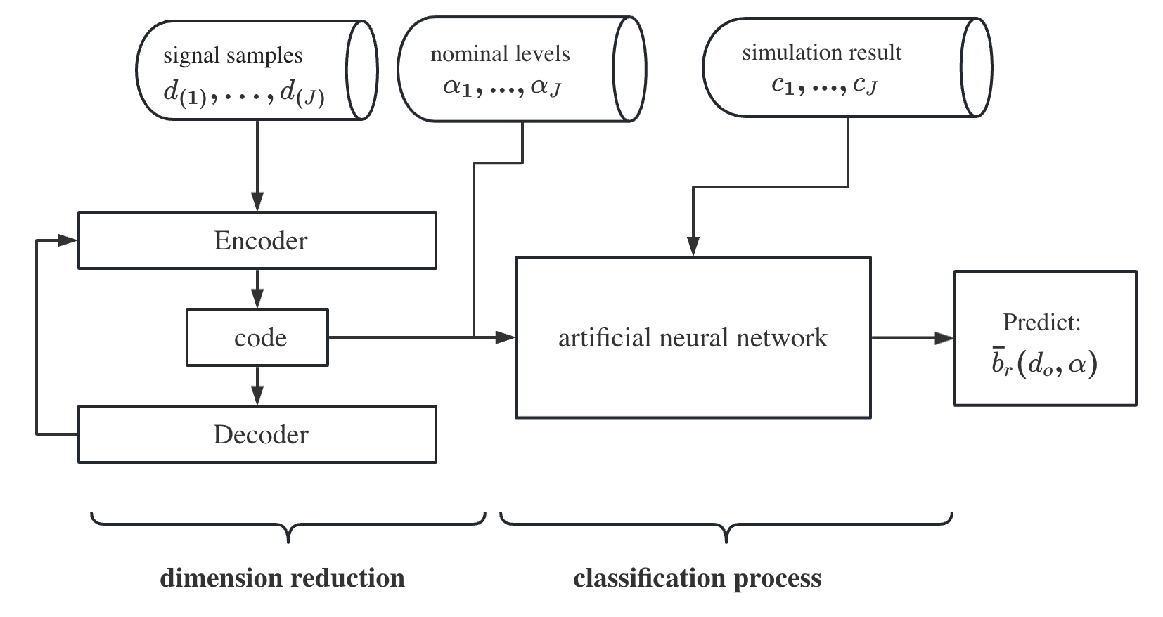
Figure 1: The flow chart describing the overall procedure of our operational coverage estimator. For $j=1,...,J$, generate $\boldsymbol{\theta}_{(j)}\sim p(\boldsymbol{\theta})$ and data streams generated using an exact model with noise $d_{(j)}=h^{(X)}_{e}(t;\boldsymbol{\theta}_{(j)})+n^{(X)}(t)$ are passed into an encoder where dimensional reduction is applied. After this process, nominal levels are simulated $\alpha_{j}\sim p(\alpha)$ and $\widehat{C}_{d_{(j)},\alpha_{j}}$ of an approximate posterior distribution using the Fisher based parameter estimation scheme returns $c_{j}$, where $c_{j}=1$ if $\boldsymbol{\theta}_{(j)}\in\widehat{C}_{d_{(j)},\alpha_{j}}$ and 0 otherwise. The classifier is subsequently trained, enabling us to predict $\bar{b}_{r}(d_{o},\alpha)$ at a specified nominal level $\alpha$.

We should point out that data stream $d_{(j)}$, as an input of the proposed classifier, can be either an actual signal ($h_{e}+n$) or discrete Fourier transform of signal ($\hat{h}_{e}+\hat{n}$). Alternatively, an adequate summary of signals can be used, and it is denoted by $S(d_{(j)})$. If a summary is used, the training set is $\{S(d_{(j)}),c_{j},\alpha_{j}\}^{J}_{j=1}$ and, the prediction is made with a nominal level of $\alpha$ and the summary of the observed data, $\bar{b}_{r}(S(d_{o}))$. Our choice of the summary for numerical simulation studies are included in Section IV and V.

We use $k$-fold cross-validation to predict success probabilities $\bar{b}_{r}(d_{o})$ and class at $d_{o}$, but the uncertainty of the operational coverage estimate is not attainable (i.e., only a point estimate is available with this approach). For a simple logistic regression, the Delta method (xu2005using, ) and the bootstrap method (efron1986bootstrap, ) are therefore applied to measure the prediction errors in Section IV. We emphasize here that there does not exist any unbiased and universal estimator of the variance of $k$-fold cross-validation that is valid under all distributions (Bengio2004, ).

III.3 Credible interval calibration via operational coverage estimation

There are no formal guidelines on how to interpret operational coverage. One may consider correcting an approximate posterior distribution. Within the Approximate Bayesian Computation (ABC) framework, adjustment procedures for bias and frequentist coverage of Bayesian credible sets were suggested when the credible set does not have the correct nominal coverage probability in the frequentist sense (menendez:2014, ). With a focus on coverage in the Bayesian sense, a distortion map estimator using machine learning methods was proposed by (xing:2020, ), and is limited to one-dimensional problems.

The application of an operational coverage estimator enables us to determine the approximate credible set level that yields the desired posterior coverage level. Since an exact inverse map of the trained ANN is not always feasible or necessary, the simplest way is to read off from a plot of operational coverage estimates against nominal values at observed signal $d_{o}$.

We construct the calibration curve for an observed signal $d_{o}$ that the nominal level is parameterized by operational coverage and the procedure is summarized in Figure 2. The training data $\{\alpha_{j},\bar{b}_{r,j}(d_{o})\}_{j=1}^{M}$ is constructed by finding the operational coverage at each of the $M$ nominal levels in $[\alpha_{\min},\alpha_{\max}]$ from the estimator (Figure 1). Taking a nominal level ($\alpha_{j}$) as a response and operational coverage ($\bar{b}_{r,j}(d_{o})$) as a predictor, the $K$-degree polynomial regression is fitted. The value for $K$ is chosen by minimizing the residual mean squared error, i.e.,

$$\alpha_{j}=c_{0}+\sum_{k=1}^{K}c_{k}\bar{b}_{r,j}(d_{o})^{k}\,,\hskip 14.22636ptj=1,...,M\,.$$

Given the desired operational coverage $b(d_{o})$, the calibrated nominal coverage level, $\widehat{\alpha}$, is estimated from the calibration curve for $d_{o}$ and, with the calibrated approximate credible set $\widehat{C}_{d_{o},\hat{\alpha}}$, $P(\theta\in\widehat{C}_{d_{o},\hat{\alpha}})=b(d_{o})$.

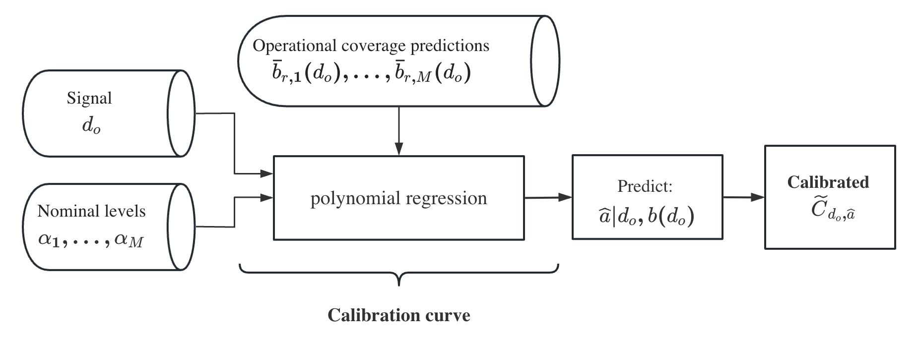
Figure 2: The flow chart describes the overall procedure of the calibration curve. After the procedure given in Figure 1 is completed, for a nominal level sample $\alpha_{j}\sim p(\alpha)$ the operational coverage is predicted $\bar{b}_{r,j}(d_{o})$ using the estimator, $j=1,...,M$. Taking $\bar{b}_{r,j}(d_{o})$ as a predictor and $\alpha_{j}$ as a response, polynomial regression is fitted then the calibrated nominal level $\widehat{\alpha}$ is predicted at the desired operational coverage $b(d_{o})$.

We demonstrate how to estimate an operational coverage and calibrate a credible set using a simple toy example in Section IV and a massive black hole problem in Section V.

IV Application: Simple toy model

In this section, we present a simple toy model to illustrate our calibration procedure discussed in section III.

IV.1 Set up and Fisher matrix validation

In this section, we will consider a data stream of the form

$$d(t)=h_{e}(t;\boldsymbol{\theta})+n(t)$$ (30)

with an exact template of the form

$$h_{e}(t;a_{0},f_{0},\dot{f}_{0})=a_{0}\sin\left(2\pi t\left[f_{0}+\frac{1}{2}\dot{f}_{0}t\right]\right).$$ (31)

Here, we have the true values for parameters $\boldsymbol{\theta}_{0}=\{a_{0}=5\cdot 10^{-21},f_{0}=10^{-3}\,\text{Hz},\dot{f}_{0}=10^{-8}\,\text{Hz}/\text{s}\}$.

We use model templates

$$h_{m}(t;a,f,\dot{f},\epsilon)=a\sin\left(2\pi t\left[f+\frac{1}{2}\dot{f}t\right](1-\epsilon)\right).$$ (32)

Here $\epsilon\ll 1$ is used as a tuneable parameter allowing deviations from the exact model (31) $h_{\text{e}}(t;\boldsymbol{\theta},\epsilon=0)$ given by an approximate model $h_{\text{m}}(t;\boldsymbol{\theta},\epsilon\neq 0)$. For simplicity, we do not take into account the response function through TDI as outlined in section II. Hence, when calculating the inner product (6), which is used in likelihood (5), Fisher matrix (16) and SNR (8) calculations, we only consider a single data stream and use the approximate LISA-like PSD defined by Equation (1) of robson2019construction .

Using equations (11a) and (11b), we generate stationary Gaussian noise in the frequency domain to construct the toy model data stream (30). In this example, we will set $\epsilon=10^{-6}$, allowing for a discrepancy between the exact model $h_{e}$ and approximate model $h_{m}$. For $\epsilon=0$ and over a time of observation of 30 hours sampled with cadence $\Delta t\sim 200\,$ seconds, we observe an optimal matched filtering SNR $\rho\sim 188$. The length of the data stream is $N=2^{16}$.

Our calibration technique requires multiple parameter estimation simulations using an approximate model to then estimate the operational coverage. As discussed in section I, this is extremely computationally intensive so we approximate samples from the approximate posterior density using a Fisher matrix approach instead.

To validate our Fisher matrix approach, we inject an exact model with $\epsilon=0$ and recover with an approximate model with $\epsilon=10^{-6}$ using the emcee algorithm. We generate 31,000 samples from the approximate posterior under $h_{m}(t;\boldsymbol{\theta}),\epsilon=10^{-6})$, and then discard 6,000 samples as burn-in. In parallel, we compute the Fisher matrix (16) and then sample from a multivariate Gaussian

$$\begin{split}\boldsymbol{\theta}&\sim\mathcal{N}\left(\boldsymbol{\theta}_{0}+\boldsymbol{\theta}_{\text{bias}},\Gamma^{-1}(h_{m})\right)\,,\\ \theta^{i}_{\text{bias}}&=[\Gamma^{-1}(h_{m})]^{ij}(\partial_{j}h_{\text{m}}|\delta h+n)\,,\end{split}$$ (33)

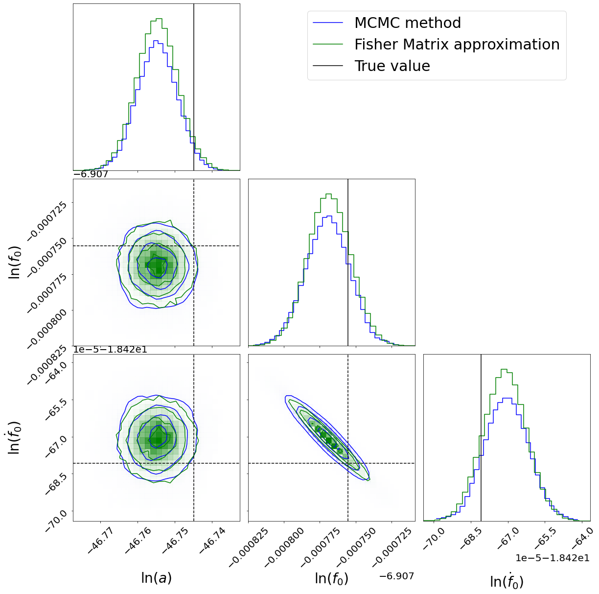
Figure 11: The blue curve represents a posterior distribution on parameters $\boldsymbol{\theta}$ when inferring parameters of an injected exact signal $h_{e}(t;\boldsymbol{\theta}_{0})$ into Gaussian noise with an approximate model template $h_{m}(t;\boldsymbol{\theta},\epsilon=10^{-6})$. The green curve represents an approximation to the posterior, computed via the Fisher matrix formalism. We highlight here that the computation of the Fisher matrix accurately describes the posterior, implying we are not subject to numerical instabilities when calculating derivatives/inverses. The black line indicates the value of the true parameters in the study.

with $\theta^{i}\in\boldsymbol{\theta}_{\text{bias}}$. Here equation (33) is evaluated at the true parameters $\boldsymbol{\theta}_{0}$ and $\delta h=h_{e}(t;\boldsymbol{\theta}_{0})-h_{m}(t;\boldsymbol{\theta}_{0},\epsilon=10^{-6})$. We plot the approximate posterior densities in Figure 11. The blue curve is generated via MCMC and the green curve generated via the Fisher matrix computation. This simulation has shown that the Fisher matrix can be used as a suitable approximation to the posterior density. Having verified the Fisher matrix is a suitable approximation, we then use it to generate approximate posteriors in bulk in order to apply the calibration procedure discussed in III. This is the focus of the next section.

IV.2 Calibration procedure

The calibration technique described in section III requires a training set, built from the prior space of samples and the resultant generation of a family of approximate posteriors. We first focus our attention on a single-parameter study, then generalise to the three-parameter study at the end of this section.

For a single-parameter study, $\dot{f}$ is unknown and the true values for $a,f$ are used. i.e., $\boldsymbol{\theta}=\dot{f}$. The uniform prior is assigned for $\dot{f}$,

$$\dot{f}\sim\text{U}[\dot{f}_{0}-10^{-13},\dot{f}_{0}+10^{-13}]\,\text{Hz/s}\,.$$ (34)

The training data $\{S(d_{(j)}),c_{j},\alpha_{j}\}^{5000}_{j=1}$ is generated to obtain a practical operational coverage estimator. For $j=1,...,5000$, $\boldsymbol{\theta}_{(j)}$ is generated from the prior (34) and $\alpha_{j}\sim U[0.78,0.97]$. For each of prior sample $\boldsymbol{\theta}_{(j)}$, the data stream $d_{(j)}=\hat{h}_{e,(j)}(f;\boldsymbol{\theta}_{(j)})+\hat{n}_{(j)}$ is generated by adding a noise $\hat{n}_{j}$ through (10) to the exact reference signal $\hat{h}_{e,(j)}$. An approximate posterior density is in the form of a multivariate Gaussian (33) using the inverse Fisher matrix (21) and expectation for the bias (17) at $\boldsymbol{\theta}_{(j)}$. An output $c_{j}$ is obtained from the $\alpha_{j}$ credible set of the approximate posterior density. Instead of $d_{(j)}$, the real part of discrete Fourier transform of signal is used to find the practical operational coverage estimator. i.e, $S(d_{(j)})=Re(d_{(j)})$. We tried $|d_{(j)}|^{2}$ and $|d_{(j)}|$ and did not gain any improvement in the results.

We use autoencoders to reduce the dimension of $S(d_{(j)})$ in order to apply the calibration procedure. The autoencoder is trained with an Adam optimizer (Kingma:2014, ) and a learning rate, $10^{-4}$, is chosen by minimizing the mean squared error. The size of $S(d_{(j)})$ is then reduced from $2^{16}$ to $2^{3}$, which is far less than the size of the overall training data set. From our preliminary study, reducing the size of the data set any less than $2^{3}$ gave a significantly poor fit. For classification, an artificial neural network (ANN) with one fully-connect layer is trained using the cross entropy loss function. The calibration curve is obtained from the feed-forward ANN inversion. We tried multiple layers for the ANN but found no real gain from using more than one layer for this toy example.

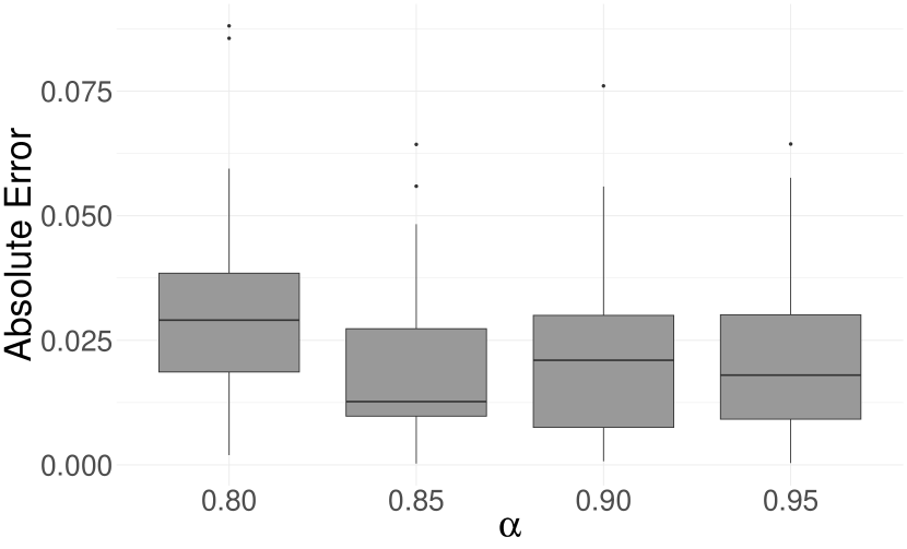
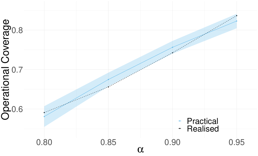
Figure 3: Estimation of $\dot{f}$-only. Absolute error from 30 replicates against $\alpha$ (left) and operational coverage estimates $\bar{b}_{r}(S(d_{o}))$ with 2-SE error and realised operational coverage $b_{r}(d_{o})$ (right) for the test waveform $d_{o}$.

The left panel of Figure 3 presents the performance of the operational coverage estimator (with summary of the procedure given in Figure 1) using 30 approximate signals with noise and on average absolute errors are relatively small. The right panel of Figure 3 compares the operational coverage estimates using the practical estimator $\bar{b}_{r}(S(d_{o}))$ (Section III.2 and the realised operational coverage $b_{r}(d_{o})$ (29) for the test signal. At a given nominal level $\alpha$, the practical operational coverage and the realised operational coverage agree to excellent precision. Absolute errors tend to be less than 0.06 in general and, for the test data, the coverage of posterior density over the 0.9 approximate credible set is 0.76.

Exact and approximate inferences on the true signal (31) are compared in Figure 4. It is observed that the exact and approximate posterior densities do not overlap completely and some deviation between them. The calibration curve shows how the calibrated level changes with the desired operational coverage and the calibrated level $\widehat{\alpha}$ is higher than $b(d_{o})$. i.e., $\bar{b}_{r}(S(d_{o}))$ is smaller than $\alpha$ (right panel of Figure 3). The main conclusion of this study is that we have calibrated an approximate credible set (arising from an approximate posterior) to achieve 0.76 coverage of the posterior.

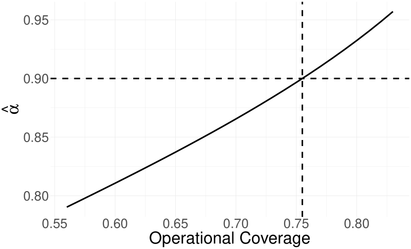
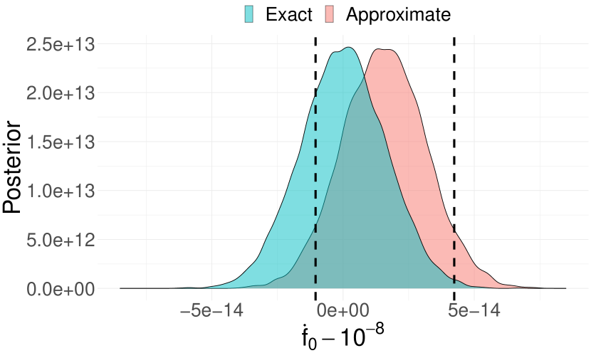
Figure 4: Left panel: Calibration curve. Right panel: Exact and approximate posterior densities of $\dot{f}_{0}$. The dashed lines on the top figure represent the operational coverage for the 90% credible interval of approximate posterior ($\widetilde{C}_{d_{o},0.9}$). This is calculated by using the calibration curve to map the calibrated nominated level of $\hat{\alpha}=90\%$ back to an operational coverage level, which is $\approx 76\%$ for the test waveform.

We now consider the full model with three parameters. i.e., $\boldsymbol{\theta}=\{a_{0},f_{0},\dot{f}_{0}\}$. Tight priors are assigned on these three parameters

$$a \sim\text{U}[a_{0}-10^{-22},a_{0}+10^{-22}]$$

$$f \sim\text{U}[f_{0}-10^{-7},f_{0}+10^{-7}]\,\text{Hz}$$

$$\dot{f} \sim\text{U}[\dot{f}_{0}-10^{-13},\dot{f}_{0}+10^{-13}]\,\text{Hz}/\text{s}.$$

We increase the size of the training data to 10,000, $\{S(d_{(j)}),c_{j},\alpha_{j}\}_{j=1}^{10000}$ where $S(d_{(j)})=\text{Re}(d_{(j)})$ and it is generated similarly. For approximate posterior density, the multivariate Gaussian form of density approximation for logged parameter values was imposed. We used three fully connected layers with one dropout layer in both the encoder and decoder to reduce the dimension of $S(d_{(j)})$ from $2^{16}$ to $2^{6}$. A 1-layer ANN classifier with the $l_{1}$ penalty on weights of neurons is fitted.

The performance of the operational coverage estimator using 30 approximate signals with noise is shown in the left penal of Figure 5 and absolute errors are less than $\approx$0.075 in general. The right penal of Figure 5 compares $\bar{b}_{r}(S(d_{o}))$ and $b_{r}(d_{o})$ for the test signal. The practical and realised operational coverage agree relatively well at a given $\alpha$. Exact and approximate posterior densities for the test data $d_{o}$ are compared in Figure 6. Calibration curve for the test waveform $d_{o}$ is shown in Figure 7 and the calibrated nominal level $\widehat{\alpha}$ is higher than the desired operational coverage value, i.e., $b_{r}(d_{o})$ is smaller than $\alpha$. For $d_{o}$, the coverage of posterior density over the approximate credible set with a nominal level of 0.89 is 0.8.

Having demonstrated our calibration procedure through an illustrative example, we will now apply it to a more realistic gravitational-wave scenario.

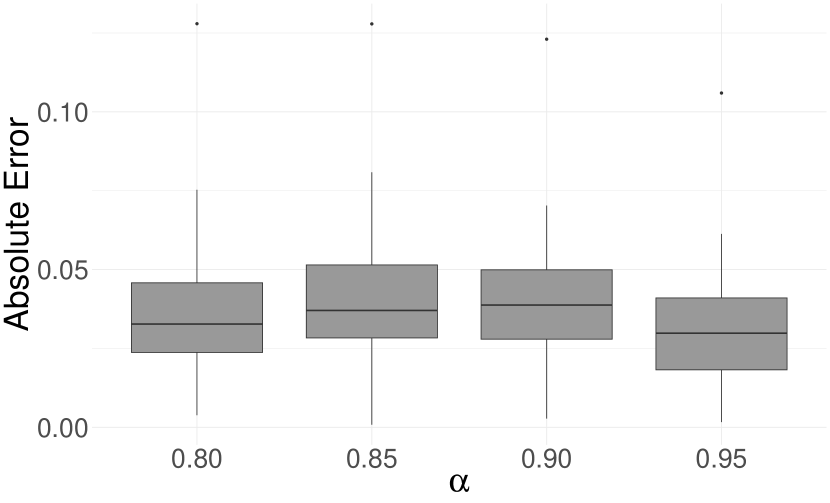
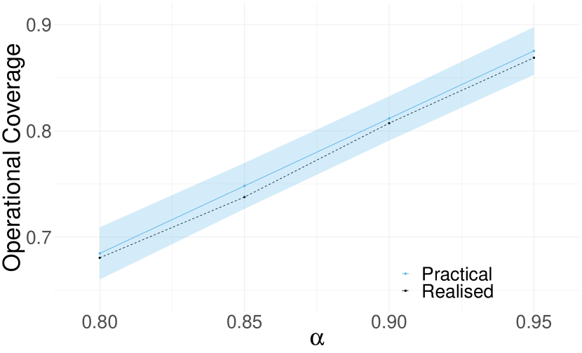
Figure 5: Estimation of the full model, i.e. $a_{0},f_{0},\dot{f}_{0}$. Absolute error from 30 replicates against $\alpha$ (left) and operational coverage estimates $\bar{b}_{r}(S(d_{o}))$ with 2-SE error and realised operational coverage $b_{r}(d_{o})$ (right) for the test waveform $d_{o}$.

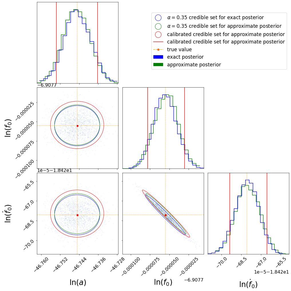
Figure 6: Corner plot summary of samples from the exact and approximate posterior densities in the toy model

. The panels on the diagonal show the exact (blue) and approximate (green) empirical marginal posterior densities with the true value (yellow dashed line) and calibrated approximate credible interval (red line). The off-diagonal panels shows the exact (blue contour) and approximate (green contour) credible sets with a nominal level of $\alpha=0.8$ and, calibrated approximate credible set (red contour) with the desired operational coverage of 0.8 based on exact (blue points) and approximate (green points) posterior sample. The true values $\boldsymbol{\theta}_{0}$ are marked by red points.

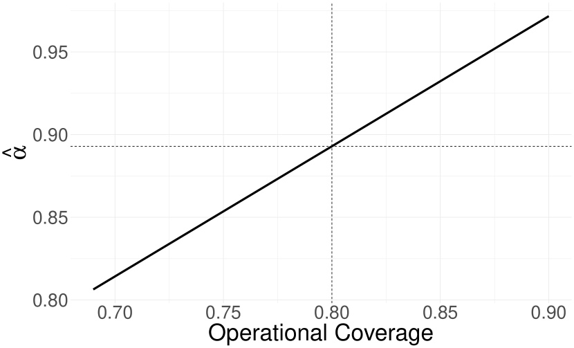
Figure 7: Calibration curve for $d_{o}$. The dashed lines represent the calibrated nominal level $\widehat{\alpha}=0.89$ for the target operational coverage $b(d_{o})=0.8$.

V Application: Massive black holes

In this section, we apply the calibration procedure discussed in section III and exemplified in section IV on a realistic massive black hole binary signal. Using lisabeta developed in marsat2021exploring ; marsat2018fourier , we generate complete inspiral-merger-ringdown frequency domain spin-aligned massive black holes in the solar system barycenter frame with the LISA response applied.

V.1 Set up

In the Bayesian inference, we incorporate higher modes $\mathcal{H}_{e}=\{(2,2),(2,1),(3,3),(3,2),(4,4),(4,3)\}$ for the true MBH waveform denoted by $h_{e}(t;\boldsymbol{\theta})$. Approximate waveforms denoted by $h_{m}(t;\boldsymbol{\theta})$ are generated by removing a single harmonic $\mathcal{H}_{m}=\mathcal{H}_{e}\backslash\{(4,3)\}$, giving a deviation from the exact model and the approximate model. For our exact signal with modes $\mathcal{H}_{e}$, we define the true parameters: the total mass $M=m_{1}+m_{2}=3\cdot 10^{7}M_{\odot}$; mass ratio $q=m_{1}/m_{2}=2$; the two effective spin parameters of the two component masses $\chi_{1}=0.5$ and $\chi_{2}=0.5$; the time of coalescence $t_{c}=10^{5}\,$seconds; luminosity distance $6.67\,$ Gpc; initial phase at coalescence $\phi_{c}=1.1$; sky position $(\beta=0.3,\lambda=0.8)$ in ecliptic coordinates; and polarisation angle $\psi=1.7$. In our example, we will focus on a subset of parameters $\boldsymbol{\theta}=\{M,q,\chi_{1},\chi_{2},t_{c}\}$, to demonstrate the calibration procedure as a proof of principle.

We choose true parameters given by $\boldsymbol{\theta}_{0}=\{M_{0}=10^{7}M_{\odot},q_{0}=2,\chi_{1,0}=0.5,\chi_{2,0}=0.5,t_{c,0}=10^{5}\,\text{seconds}\}$. The observation time of our signals will be $\sim 1$ day, sampled with cadence $\Delta t=200$ seconds. Due to the large total mass, the frequencies emitted by the massive black hole signal are low, even at the larger harmonics. This allows us to analyse very short data segments with large sampling intervals thus reducing computational costs. The length of our data sets are $N=2^{12}$. We found that the optimal matched filtering SNR using (8) over both the A and E channels are given by $\rho_{A}\sim 2022.02$ and $\rho_{E}\sim 1702.57$ giving a total SNR over both A and E as $\rho_{AE}\sim 2643.35$.

Before applying the calibration procedure, we will show that our Fisher matrix calculations are not subject to numerical instabilities. We inject a signal with true parameters $\boldsymbol{\theta}_{0}$ defined earlier into a two noiseless data streams corresponding to TDI channels $X=\{A,E\}$. Including the $T$ channel is unnecessary for our purposes since the contribution of SNR is low with respect to the $A$ and $E$ channels. For inference, we use the likelihood defined in (7) with model template $h_{m}$ with an incomplete set of modes $\mathcal{H}_{m}=\mathcal{H}_{e}/\{(4,3)\}$. Starting close to the true parameters, we use the emcee sampling algorithm to generate samples from the approximate posterior density $\tilde{p}(\boldsymbol{\theta}|d)$. To compute the Fisher matrix, we use the numerical procedure of finite differences to compute derivatives of the MBH waveform with respect to parameters. After computing the matrix (16), we apply a log-transformation to reduce the condition number of the matrix prior to computing the inverse. From equation (20), we then sample from a multivariate Gaussian

$$\begin{split}\boldsymbol{\theta}&\sim\mathcal{N}\left(\boldsymbol{\theta}_{0}+\boldsymbol{\theta}_{\text{bias}},\Gamma_{AE}^{-1}(h_{m})\right)\,,\\ \theta^{i}_{\text{bias}}&=[\Gamma_{AE}(h_{m})^{-1}]^{ij}\sum_{X=\{A,E\}}(\partial_{j}h^{(X)}_{\text{m}}|\delta h^{(X)}+n^{(X)})\end{split}$$ (35)

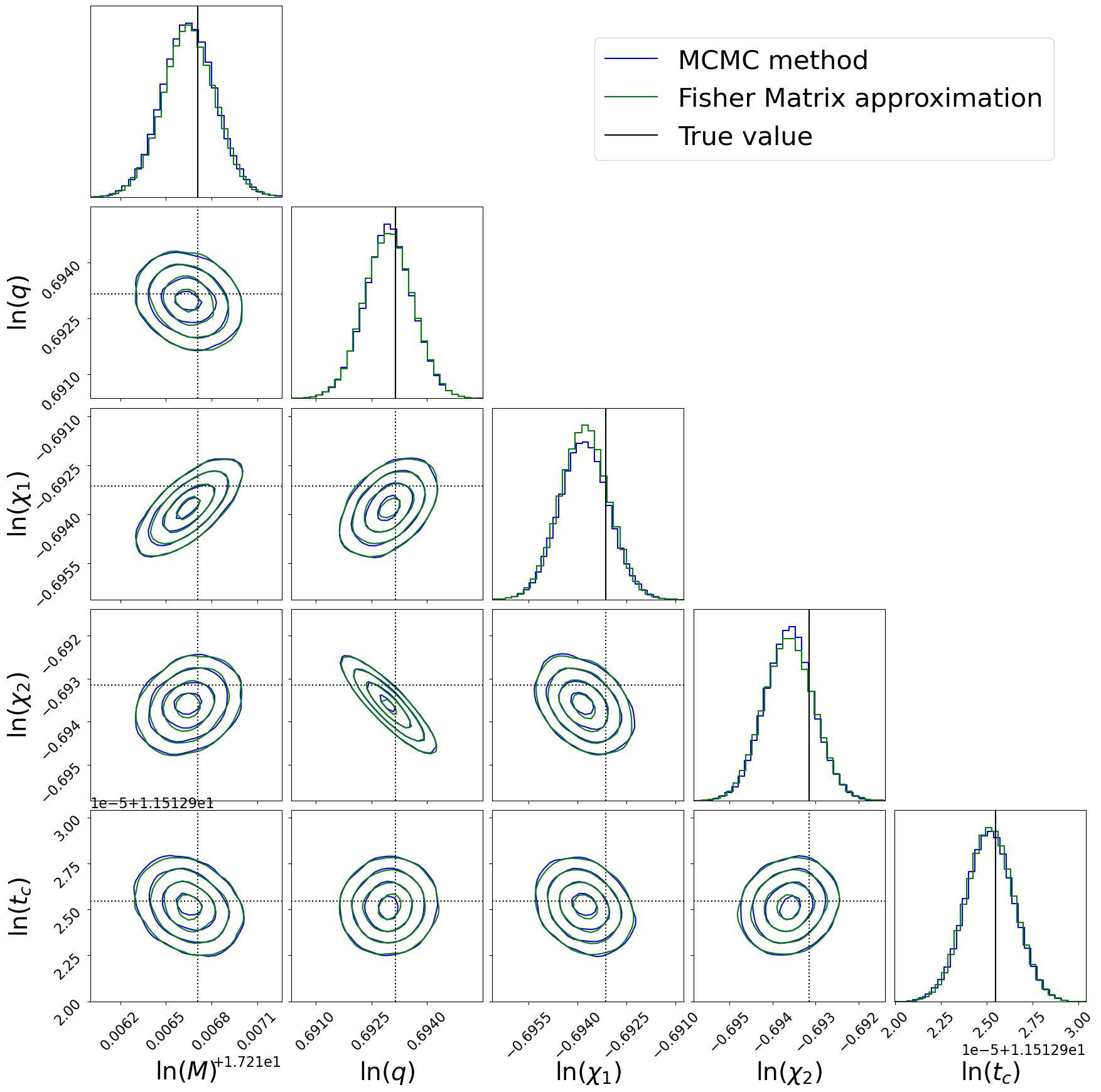
Figure 12: Comparison of posterior distribution between the MCMC method (blue) and the Fisher Matrix approximation (green) at the massive black hole binary signal $d_{o}$, with black vertical/horizontal lines denoting the true parameters. We highlight here an excellent agreement between our MCMC simulation and the approximate Fisher matrix approach. We see that both the fluctuations to recovered parameters (induced through noise via equation (18) and precision measurements on parameters encoded by (16) are well described by the Fisher matrix formalism.

for $\theta^{i}_{\text{bias}}$ a component of $\boldsymbol{\theta}$. We remind the reader that each of the quantities in (35) is evaluated at the true parameters $\boldsymbol{\theta}$. We then plot the histogram of samples alongside the approximate posterior density in Figure 12. What we learn here is that the Fisher matrix is a suitable approximation to the posterior density and can be used to approximate posterior distributions generated using an approximate waveform model.

V.2 Calibration Procedure

As a proof of principle, we will apply our calibration procedure on a five-dimensional space. We will choose the five parameter set $\boldsymbol{\theta}=\{M,q,\chi_{1},\chi_{2},t_{c}\}$. For this study, tight uniform priors are set for the five parameters as follows:

$$M \sim \text{U}[M_{0}-5\times 10^{4},M_{0}+5\times 10^{4}]$$

$$q \sim \text{U}[q_{0}-2.5\times 10^{-3},q_{0}+2.5\times 10^{-3}]$$

$$\chi_{1} \sim \text{U}[\chi_{1,0}-5\times 10^{-4},\chi_{1,0}+5\times 10^{-4}]$$

$$\chi_{2} \sim \text{U}[\chi_{2,0}-5\times 10^{-4},\chi_{2,0}+5\times 10^{-4}]$$

$$t_{c} \sim \text{U}[t_{c,0}-0.25,t_{c,0}+0.25].$$

Following a similar procedure outlined in IV.2, the data stream is $d=\hat{h}_{e}(\boldsymbol{\theta})+\hat{n}$ and the test waveform is $d_{o}=\hat{h}_{e}(\boldsymbol{\theta}_{0})$. The training data $\{S(d_{(j)}),c_{j},\alpha_{j}\}^{10^{5}}_{j=1}$ where $S(d_{(j)})=\text{Re}(d_{(j)})$ is generated to get a practical operational coverage estimator. We also considered $|d_{(j)}|^{2}$ and did not gain any significant improvements in the results and, the corresponding result is not included in the paper. We reduce the input feature size of $N=2^{12}$ to $N=2^{8}$ using a three-layer fully-connected encoder and decoder network. For classification, an ANN using three fully-connected hidden layers and an output layer with a sigmoid activation function are used. For the realized operational coverage estimation $b_{r}$, we used 26,880 exact posterior samples, using the complete IMR waveform with full harmonic structure $\mathcal{H}_{e}$, with 32 parallel chains with a thinning factor of 5.

In general, the operational coverage estimator $\bar{b}_{r}$ exhibits generally small absolute errors in Figure 8. Although the absolute errors tend to increase with $\alpha$, relative errors are likely to be less variable. The absolute error is small as 0.013 and large as 0.065. i.e., the smallest and largest relative absolute errors are $0.013/0.6=0.0217$ and $0.065/0.99=0.0657$ respectively. For the test waveform $d_{o}$, the estimate $\bar{b}_{r}(S(d_{o}))$ from the practical operational estimator is compared to the realistic operational coverage $b_{r}(d_{o})$ in the top plot of Figure 9. The calibration curve in Figure 9 was modelled by a polynomial regression with the degree 7. We observe a very small operational coverage in comparison to the nominal level ($\bar{b}_{r}(S(d_{o}))\ll\alpha$), and this is due to the small overlap between the exact and approximate posterior distributions in Figure 10, in particular $q$ and $\chi_{2}$. For example, the posterior coverage of the 0.967 credible set of an approximate posterior distribution is 0.35 and this is also confirmed from the calibration curve that the calibrated level is 0.97 for the target operational coverage of 0.35. As result, the calibrated credible set of an approximate posterior (red contour) is larger in order to achieve the target 0.35 operational coverage, which is about 1.8$\sigma$.

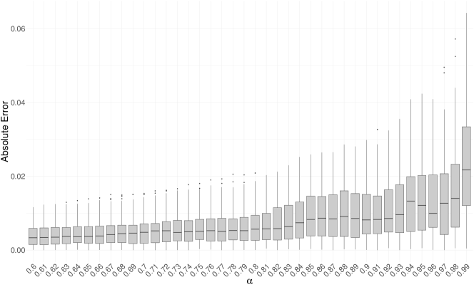
Figure 8: Absolute error between operational coverage estimate and realised operational coverage against $\alpha$ from 30 replicates. The black dots are outlier absolute errors at a specific nominal level $\alpha$.

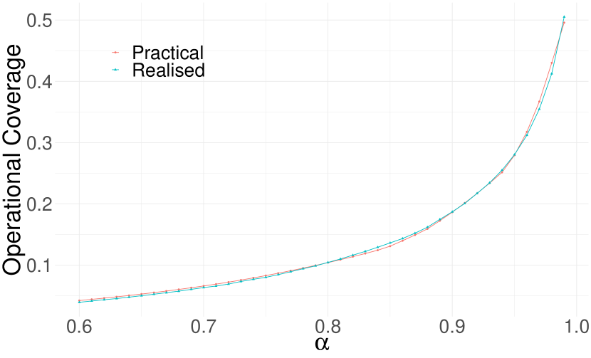
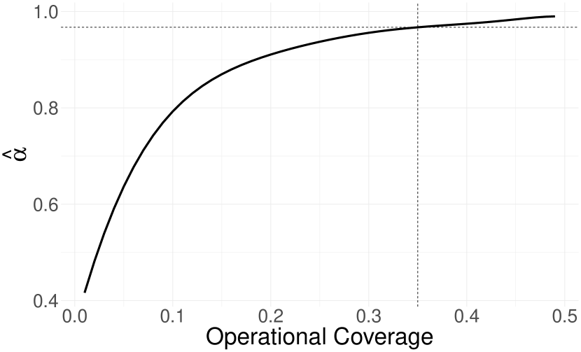
Figure 9: Top panel: Operational coverage estimates $\bar{b}_{r}(S(d_{o}))$ (red) and realised operational coverage $b_{r}(d_{o})$ (blue) for the test data $d_{o}$ against $\alpha$. Bottom panel: Calibration curve for $d_{o}$ (Calibrated nominal levels $\widehat{\alpha}$ against the target operational coverage $b(d_{o})$). The dashed lines represent the calibrated nominal level $\widehat{\alpha}=0.97$ for the target operational coverage $b(d_{o})=0.35$.

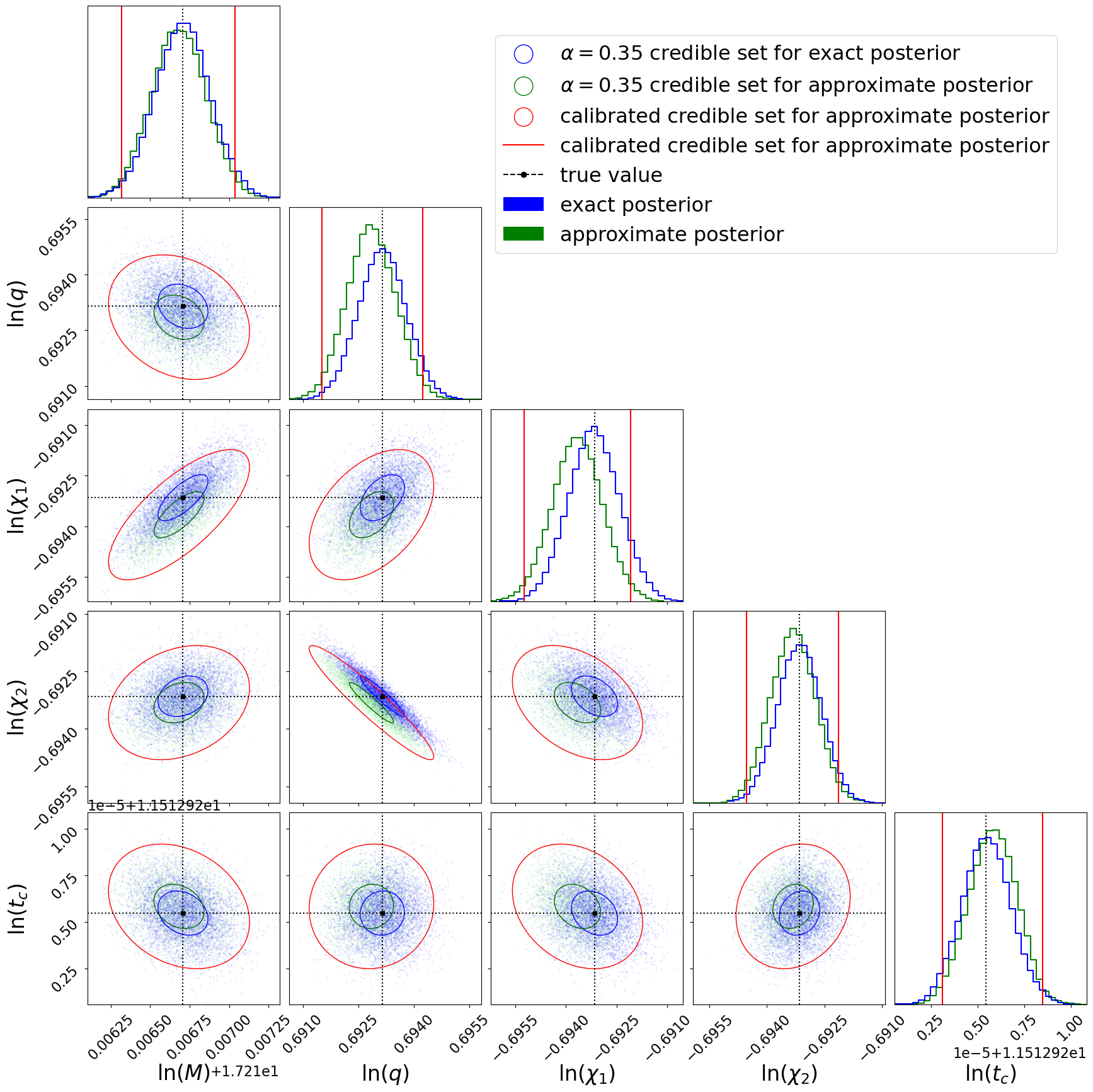
Figure 10: Corner plot summary of samples from the exact and approximate posterior densities for the massive black hole binary signal $d_{o}$. The panels on the diagonal show the exact (blue) and approximate (green) empirical marginal posterior densities with the true value (black dashed line) and calibrated approximate credible interval (red line). The off-diagonal panels show the exact (blue contour) and approximate (green contour) credible set with a nominal level of $\alpha=0.35$ and, the calibrated approximate credible set (red contour) with the desired operational coverage of $0.35$ based on exact (blue points) and approximate (green points) posterior samples. The true values $\boldsymbol{\theta}_{0}$ are marked by black points.

VI Discussion and conclusions

In this paper, we have presented a Bayesian calibration procedure for the operational coverage of an approximate family of GW posteriors and applied the method to both a toy model and a more realistic analysis of MBHB signals for LISA. Specifically, the posteriors that are calibrated in our work are Fisher-information-based approximations (i.e., normal approximations) to the posteriors that are obtained by using an approximate waveform model in the GW likelihood. Such approximations are frequently used in GW astronomy to perform bulk calculations in exploratory data analysis studies; our proposed method then allows users to rapidly obtain corrected credible sets that correspond to some desired coverage level (“correct” relative to a more accurate waveform model).

At present, our proposed method is novel in the GW literature and has no comparable counterpart since other methods for inference calibration i) focus on correcting the posterior itself in terms of coverage and ii) deal only with a single posterior at a time. For example, one would have to evaluate the accurate model in bulk in order to use the method proposed by Cutler and Vallisneri Cutler:2007mi for estimating inference biases on the fly. Even if a regression model is fit directly to the biases over the waveform model space, that would still require learning a parameter vector rather than a single coverage number, which would require more complex computation and stringent accuracy requirements on the fit.

In addition to our proposed usage of the method in bulk studies over a space of GW signals, the calibration procedure could potentially also be used on actual data containing a signal. With a model that is pre-trained on more accurate waveforms and realistic detector noise, one could rapidly compute calibrated credible sets for the approximate waveforms used in template banks for ground-based observing. This could be useful for applications such as the rapid sky localisation of sources for low-latency electromagnetic follow-up. The future third-generation ground-based GW detectors, such as the Einstein Telescope and Cosmic Explorer, will have enhanced sensitivity to gravitational wave signals in the Hz frequency band $f\in(5,2000)\,\text{Hz}$. These instruments can exploit the proposed operational coverage discussed in this paper in order to quantify the systematic biases and thus investigate the impact of inaccurate waveforms on tests of GR in an efficient way PhysRevResearch.2.023151 . The estimated operational coverage can be regarded as a criterion to set requirements for the sensitivity of the detectors to yield unbiased parameter inference for the target system. The forward-thinking calibrated result gives reasonable and meaningful information for future GW research.

The MBH example we presented was restricted to five parameters of the full waveform model. However, the computational complexity of the calibration procedure — in particular, the operational coverage estimator — will typically require a significant increase in computing resources as additional parameters are considered. Increasing the computational efficiency of the operational coverage estimator for high-dimensional problems, and thus improving the scalability of the calibration method to the dimensionalities of both the parameter space and the data representation, is an avenue for future research.

We should point out that the approximate posterior distribution is not too different to the true one. At least, the overlap of the credible intervals exists, which is not always the case. As the divergence between posteriors becomes large, the nominal credible level to achieve any operational coverage goes to 1, which is trivial and manifests the inability to train the model. Therefore, it is encouraged to estimate the maximum operational coverage when obtaining the calibration curve; if it is small, for example, less than $0.5\sigma$, more accurate waveforms should be considered.

The Python code for the one-dimensional toy example in Section IV is provided at https://github.com/bpandamao/calibration_case_study.

Author Contributions

R. Mao: Conceptualization, Data curation, Formal analysis, Investigation, Methodology, Project administration, Resources, Software, Supervision, Validation, Visualization, Writing – original draft.

JEL: Conceptualization, Data curation, Investigation, Methodology, Project administration, Resources, Software, Supervision, Validation, Visualization, Writing – original draft.

OB: Conceptualization, Data curation, Formal analysis, Investigation, Software: Fisher matrix, MCMC & lisa-beta, Methodology, Resources, Software, Supervision, Validation, Visualization, Writing – original draft.

AJKC: Conceptualization, Formal analysis, Methodology, Project administration, Supervision, Writing – original draft, Writing - Review & Editing.

MCE: Conceptualization, Methodology, Project Administration, Software, Visualization, Writing - Original Draft, Writing - Review & Editing.

R. Meyer: Conceptualization, Methodology, Funding acquisition, Project Administration, Supervision, Writing - Original Draft, Writing – Review & Editing.

Appendix A Fisher matrix computations

References

- [1] Benjamin P Abbott, Richard Abbott, TDe Abbott, MR Abernathy, Fausto Acernese, Kendall Ackley, Carl Adams, Thomas Adams, Paolo Addesso, RX Adhikari, et al. Observation of gravitational waves from a binary black hole merger. Physical review letters, 116(6):061102, 2016.
- [2] John Veitch, Vivien Raymond, Benjamin Farr, Will Farr, Philip Graff, Salvatore Vitale, Ben Aylott, Kent Blackburn, Nelson Christensen, Michael Coughlin, et al. Parameter estimation for compact binaries with ground-based gravitational-wave observations using the lalinference software library. Physical Review D, 91(4):042003, 2015.
- [3] Benjamin P Abbott, Rich Abbott, Thomas D Abbott, Sheelu Abraham, Fausto Acernese, Kendall Ackley, Carl Adams, Vaishali B Adya, Christoph Affeldt, Michalis Agathos, et al. A guide to ligo–virgo detector noise and extraction of transient gravitational-wave signals. Classical and Quantum Gravity, 37(5):055002, 2020.
- [4] Benjamin P Abbott, R Abbott, TD Abbott, MR Abernathy, F Acernese, K Ackley, C Adams, T Adams, P Addesso, RX Adhikari, et al. Gw150914: First results from the search for binary black hole coalescence with advanced ligo. Physical Review D, 93(12):122003, 2016.
- [5] Prayush Kumar, Ilana MacDonald, Duncan A Brown, Harald P Pfeiffer, Kipp Cannon, Michael Boyle, Lawrence E Kidder, Abdul H Mroué, Mark A Scheel, Béla Szilágyi, et al. Template banks for binary black hole searches with numerical relativity waveforms. Physical Review D, 89(4):042002, 2014.
- [6] Samantha A Usman, Alexander H Nitz, Ian W Harry, Christopher M Biwer, Duncan A Brown, Miriam Cabero, Collin D Capano, Tito Dal Canton, Thomas Dent, Stephen Fairhurst, et al. The pycbc search for gravitational waves from compact binary coalescence. Classical and Quantum Gravity, 33(21):215004, 2016.
- [7] P Ajith, N Fotopoulos, S Privitera, A Neunzert, N Mazumder, and AJ Weinstein. Effectual template bank for the detection of gravitational waves from inspiralling compact binaries with generic spins. Physical Review D, 89(8):084041, 2014.
- [8] T Adams, D Buskulic, V Germain, GM Guidi, F Marion, Matteo Montani, B Mours, Francesco Piergiovanni, and Gang Wang. Low-latency analysis pipeline for compact binary coalescences in the advanced gravitational wave detector era. Classical and Quantum Gravity, 33(17):175012, 2016.
- [9] Nelson Christensen and Renate Meyer. Parameter estimation with gravitational waves. Reviews of Modern Physics, 94(2):025001, 2022.
- [10] Renate Meyer, Matthew C Edwards, Patricio Maturana-Russel, and Nelson Christensen. Computational techniques for parameter estimation of gravitational wave signals. Wiley Interdisciplinary Reviews: Computational Statistics, 14(1):e1532, 2022.
- [11] Lee S Finn. Detection, measurement, and gravitational radiation. Physical Review D, 46(12):5236, 1992.
- [12] Mark Miller. Accuracy requirements for the calculation of gravitational waveforms from coalescing compact binaries in numerical relativity. Phys. Rev. D, 71:104016, May 2005.
- [13] Luis Lehner and Frans Pretorius. Numerical relativity and astrophysics. Annual Review of Astronomy and Astrophysics, 52:661–694, 2014.
- [14] Frans Pretorius. Numerical relativity using a generalized harmonic decomposition. Classical and Quantum Gravity, 22(2):425, 2005.
- [15] Luis Lehner. Numerical relativity: a review. Classical and Quantum Gravity, 18(17):R25, 2001.
- [16] Michael Boyle, Daniel Hemberger, Dante AB Iozzo, Geoffrey Lovelace, Serguei Ossokine, Harald P Pfeiffer, Mark A Scheel, Leo C Stein, Charles J Woodford, Aaron B Zimmerman, et al. The sxs collaboration catalog of binary black hole simulations. Classical and Quantum Gravity, 36(19):195006, 2019.
- [17] Carlos O Lousto and Yosef Zlochower. Orbital evolution of extreme-mass-ratio black-hole binaries with numerical relativity. Physical review letters, 106(4):041101, 2011.
- [18] Jonathan Blackman, Scott E Field, Chad R Galley, Béla Szilágyi, Mark A Scheel, Manuel Tiglio, and Daniel A Hemberger. Fast and accurate prediction of numerical relativity waveforms from binary black hole coalescences using surrogate models. Physical review letters, 115(12):121102, 2015.
- [19] Alessandra Buonanno and Thibault Damour. Effective one-body approach to general relativistic two-body dynamics. Physical Review D, 59(8):084006, 1999.
- [20] Alessandro Nagar and Piero Rettegno. Efficient effective one body time-domain gravitational waveforms. Physical Review D, 99(2):021501, 2019.
- [21] Roberto Cotesta, Sylvain Marsat, and Michael Pürrer. Frequency-domain reduced-order model of aligned-spin effective-one-body waveforms with higher-order modes. Physical Review D, 101(12):124040, 2020.
- [22] Sebastian Khan, Sascha Husa, Mark Hannam, Frank Ohme, Michael Pürrer, Xisco Jiménez Forteza, and Alejandro Bohé. Frequency-domain gravitational waves from nonprecessing black-hole binaries. ii. a phenomenological model for the advanced detector era. Physical Review D, 93(4):044007, 2016.
- [23] Sascha Husa, Sebastian Khan, Mark Hannam, Michael Pürrer, Frank Ohme, Xisco Jiménez Forteza, and Alejandro Bohé. Frequency-domain gravitational waves from nonprecessing black-hole binaries. i. new numerical waveforms and anatomy of the signal. Physical Review D, 93(4):044006, 2016.
- [24] Geraint Pratten, Sascha Husa, Cecilio Garcí a-Quirós, Marta Colleoni, Antoni Ramos-Buades, Héctor Estellés, and Rafel Jaume. Setting the cornerstone for a family of models for gravitational waves from compact binaries: The dominant harmonic for nonprecessing quasicircular black holes. Physical Review D, 102(6), sep 2020.
- [25] Eanna E. Flanagan and Scott A. Hughes. Measuring gravitational waves from binary black hole coalescences: 2. The Waves’ information and its extraction, with and without templates. Phys. Rev. D, 57:4566–4587, 1998.
- [26] Curt Cutler and Michele Vallisneri. LISA detections of massive black hole inspirals: Parameter extraction errors due to inaccurate template waveforms. Phys. Rev. D, 76:104018, 2007.
- [27] Qian Hu and John Veitch. Accumulating errors in tests of general relativity with gravitational waves: Overlapping signals and inaccurate waveforms. The Astrophysical Journal, 945(2):103, March 2023.
- [28] Andrea Antonelli, Ollie Burke, and Jonathan R Gair. Noisy neighbours: inference biases from overlapping gravitational-wave signals. Monthly Notices of the Royal Astronomical Society, 507(4):5069–5086, 2021.
- [29] Elia Pizzati, Surabhi Sachdev, Anuradha Gupta, and BS Sathyaprakash. Toward inference of overlapping gravitational-wave signals. Physical Review D, 105(10):104016, 2022.
- [30] Qian Hu and John Veitch. Accumulating errors in tests of general relativity with gravitational waves: Overlapping signals and inaccurate waveforms. The Astrophysical Journal, 945(2):103, 2023.
- [31] Pau Amaro-Seoane, Heather Audley, Stanislav Babak, John Baker, Enrico Barausse, Peter Bender, Emanuele Berti, Pierre Binetruy, Michael Born, Daniele Bortoluzzi, Jordan Camp, Chiara Caprini, Vitor Cardoso, Monica Colpi, John Conklin, Neil Cornish, Curt Cutler, Karsten Danzmann, Rita Dolesi, Luigi Ferraioli, Valerio Ferroni, Ewan Fitzsimons, Jonathan Gair, Lluis Gesa Bote, Domenico Giardini, Ferran Gibert, Catia Grimani, Hubert Halloin, Gerhard Heinzel, Thomas Hertog, Martin Hewitson, Kelly Holley-Bockelmann, Daniel Hollington, Mauro Hueller, Henri Inchauspe, Philippe Jetzer, Nikos Karnesis, Christian Killow, Antoine Klein, Bill Klipstein, Natalia Korsakova, Shane L Larson, Jeffrey Livas, Ivan Lloro, Nary Man, Davor Mance, Joseph Martino, Ignacio Mateos, Kirk McKenzie, Sean T McWilliams, Cole Miller, Guido Mueller, Germano Nardini, Gijs Nelemans, Miquel Nofrarias, Antoine Petiteau, Paolo Pivato, Eric Plagnol, Ed Porter, Jens Reiche, David Robertson, Norna Robertson, Elena Rossi, Giuliana Russano, Bernard Schutz, Alberto Sesana, David Shoemaker, Jacob Slutsky, Carlos F. Sopuerta, Tim Sumner, Nicola Tamanini, Ira Thorpe, Michael Troebs, Michele Vallisneri, Alberto Vecchio, Daniele Vetrugno, Stefano Vitale, Marta Volonteri, Gudrun Wanner, Harry Ward, Peter Wass, William Weber, John Ziemer, and Peter Zweifel. Laser interferometer space antenna, 2017.
- [32] John Baker, Jillian Bellovary, Peter L Bender, Emanuele Berti, Robert Caldwell, Jordan Camp, John W Conklin, Neil Cornish, Curt Cutler, Ryan DeRosa, et al. The laser interferometer space antenna: unveiling the millihertz gravitational wave sky. arXiv preprint arXiv:1907.06482, 2019.
- [33] Emanuele Berti, Vitor Cardoso, and Clifford M Will. Gravitational-wave spectroscopy of massive black holes with the space interferometer lisa. Physical Review D, 73(6):064030, 2006.
- [34] Scott A Hughes. Untangling the merger history of massive black holes with lisa. Monthly Notices of the Royal Astronomical Society, 331(3):805–816, 2002.
- [35] Alberto Sesana, Francesco Haardt, Piero Madau, and Marta Volonteri. The gravitational wave signal from massive black hole binaries and its contribution to the lisa data stream. The Astrophysical Journal, 623(1):23, 2005.
- [36] Alberto Vecchio. Lisa observations of rapidly spinning massive black hole binary systems. Physical Review D, 70(4):042001, 2004.
- [37] Neil J Cornish and Edward K Porter. The search for massive black hole binaries with lisa. Classical and Quantum Gravity, 24(23):5729, 2007.
- [38] Edward K Porter and Neil J Cornish. Effect of higher harmonic corrections on the detection of massive black hole binaries with lisa. Physical Review D, 78(6):064005, 2008.
- [39] Kent Yagi and Leo C Stein. Black hole based tests of general relativity. Classical and Quantum Gravity, 33(5):054001, 2016.
- [40] Enrico Barausse, Emanuele Berti, Thomas Hertog, Scott A Hughes, Philippe Jetzer, Paolo Pani, Thomas P Sotiriou, Nicola Tamanini, Helvi Witek, Kent Yagi, et al. Prospects for fundamental physics with lisa. General Relativity and Gravitation, 52:1–33, 2020.
- [41] Jonathan R Gair, Michele Vallisneri, Shane L Larson, and John G Baker. Testing general relativity with low-frequency, space-based gravitational-wave detectors. Living Reviews in Relativity, 16:1–109, 2013.
- [42] Christopher J. Moore and Jonathan R. Gair. Novel Method for Incorporating Model Uncertainties into Gravitational Wave Parameter Estimates. Phys. Rev. Lett., 113:251101, 2014.
- [43] Christopher J. Moore, Christopher P. L. Berry, Alvin J. K. Chua, and Jonathan R. Gair. Improving gravitational-wave parameter estimation using Gaussian process regression. Phys. Rev. D, 93(6):064001, 2016.
- [44] Alvin J. K. Chua, Natalia Korsakova, Christopher J. Moore, Jonathan R. Gair, and Stanislav Babak. Gaussian processes for the interpolation and marginalization of waveform error in extreme-mass-ratio-inspiral parameter estimation. Phys. Rev. D, 101(4):044027, 2020.
- [45] Miaoxin Liu, Xiao-Dong Li, and Alvin J. K. Chua. Improving the scalability of Gaussian-process error marginalization in gravitational-wave inference. 7 2023.
- [46] Jocelyn Read. Waveform uncertainty quantification and interpretation for gravitational-wave astronomy. Classical and Quantum Gravity, 40(13):135002, 2023.
- [47] Caroline B. Owen, Carl-Johan Haster, Scott Perkins, Neil J. Cornish, and Nicolás Yunes. Waveform accuracy and systematic uncertainties in current gravitational wave observations. Phys. Rev. D, 108:044018, Aug 2023.
- [48] M. I. Jordan, Z. Ghahramani, T. S. Jaakkola, and L. K. Saul. An introduction to variational methods for graphical models. Machine learning, 37(2):183–233, 1999.
- [49] D. J. C. Mackay. Choice of basis for laplace approximation. Machine Learning, 33:77–86, 1998.
- [50] A. M. Walker. On the asymptotic behaviour of posterior distributions. Journal of the Royal Statistical Society. Series B (Methodological), 31:80–88, 1969.
- [51] Michele Vallisneri. Use and abuse of the fisher information matrix in the assessment of gravitational-wave parameter-estimation prospects. Physical Review D, 77(4):042001, 2008.
- [52] Antoine Klein, Enrico Barausse, Alberto Sesana, Antoine Petiteau, Emanuele Berti, Stanislav Babak, Jonathan Gair, Sofiane Aoudia, Ian Hinder, Frank Ohme, and Barry Wardell. Science with the space-based interferometer eLISA: Supermassive black hole binaries. Physical Review D, 93(2), jan 2016.
- [53] Stanislav Babak, Jonathan Gair, Alberto Sesana, Enrico Barausse, Carlos F Sopuerta, Christopher PL Berry, Emanuele Berti, Pau Amaro-Seoane, Antoine Petiteau, and Antoine Klein. Science with the space-based interferometer lisa. v. extreme mass-ratio inspirals. Physical Review D, 95(10):103012, 2017.
- [54] Christopher PL Berry, Scott A Hughes, Carlos F Sopuerta, Alvin JK Chua, Anna Heffernan, Kelly Holley-Bockelmann, Deyan P Mihaylov, M Coleman Miller, and Alberto Sesana. The unique potential of extreme mass-ratio inspirals for gravitational-wave astronomy. arXiv preprint arXiv:1903.03686, 2019.
- [55] Monica Colpi, Kelly Holley-Bockelmann, Tamara Bogdanovic, Priya Natarajan, Jillian Bellovary, Alberto Sesana, Michael Tremmel, Jeremy Schnittman, Julia Comerford, Enrico Barausse, et al. The gravitational wave view of massive black holes. ArXiv. org, 2019.
- [56] Jeong Eun Lee, Geoff K. Nicholls, and Robin J. Ryder. Calibration Procedures for Approximate Bayesian Credible Sets. Bayesian Analysis, 14(4):1245 – 1269, 2019.
- [57] H. Xing, G. Nicholls, and J. Lee. Calibrated approximate bayesian inference. In Proceedings of the 36th International Conference on Machine Learning, PMLR, volume 97, pages 6912–6920, 2019.
- [58] Massimo Tinto and Sanjeev Dhurandhar. Time-delay interferometry. Living Reviews in Relativity, 24, 2021.
- [59] Massimo Tinto, Sanjeev Dhurandhar, and Dishari Malakar. Second-generation time-delay interferometry. Phys. Rev. D, 107:082001, Apr 2023.
- [60] Tyson B. Littenberg and Neil J. Cornish. Prototype global analysis of lisa data with multiple source types. Phys. Rev. D, 107:063004, Mar 2023.
- [61] Norbert Wiener et al. Generalized harmonic analysis. Acta mathematica, 55:117–258, 1930.
- [62] Alexander Khintchine. Korrelationstheorie der stationären stochastischen prozesse. Mathematische Annalen, 109(1):604–615, 1934.
- [63] Alexander Iain Burke and Ollie Burke. Extreme precision and extreme complexity: source modelling and data analysis development for the laser interferometer space antenna. 2021.
- [64] P. Whittle. Curve and periodogram smoothing. Journal of the Royal Statistical Society: Series B (Statistical Methodology), 19:38–63, 1957.
- [65] Philip M Woodward. Probability and information theory, with applications to radar: international series of monographs on electronics and instrumentation, volume 3. Elsevier, 2014.
- [66] George Turin. An introduction to matched filters. IRE transactions on Information theory, 6(3):311–329, 1960.
- [67] Daniel Foreman-Mackey, David W. Hogg, Dustin Lang, and Jonathan Goodman. emcee: The MCMC Hammer. Publications of the Astronomical Society of the Pacific, 125(925):306, March 2013.
- [68] J. K. Pritchard, S. M. T, A. Perez-Lezaun, and M. W. Feldman. Population growth of human y chromosomes: a study of y chromosome microsatellites. Molecular Biology and Evolution, 16(12):1791–1798, 1999.
- [69] J. Besag. Statistical analysis of non-lattice data. The statistician, 24(3):179–195, 1975.
- [70] S. N. Wood. Statistical inference for noisy nonlinear ecological dynamic systems. Nature, 466:1102–1104, 2010.
- [71] P. Fearnhead and D. Prangle. Constructing summary statistics for approximate bayesian computation: semi-automatic approximate bayesian computation. Journal of the Royal Statistical Society: Series B (Statistical Methodology), 74(3):419–474, 2012.
- [72] D. Prangle, M. G. B. Blum, G. Popovic, and S. A. Sisson. Diagnostic tools for approximate bayesian computation using the coverage property. Australian & New Zealand Journal of Statistics, 56(4):309–329, 2014.
- [73] Y. Yao, A. Vehtari, D. Simpson, and A. Gelman. Yes, but did it work?: Evaluating variational inference. In In Proceedings of the 35th International Conference on Machine Learning, volume 80, pages 5581–5590, 2018.
- [74] J. Geweke. Getting it right: Joint distribution tests of posterior simulators. J. Am. Stat. Assoc., 99:799–804, 2004.
- [75] S. R. Cook, A. Gelman, and D. B. Rubin. Validation of software for bayesian models using posterior quantile. J. Comput. Graph. Stat., 15:675–692, 2006.
- [76] H. Xing, G. Nicholls, and J. Lee. Distortion estimates for approximate bayesian inference. In Jonas Peters and David Sontag, editors, Proceedings of the 36th Conference on Uncertainty in Artificial Intelligence (UAI), volume 124 of Proceedings of Machine Learning Research, pages 1208–1217. PMLR, 2020.
- [77] G.E. Hintonand and R. R. Salakhutdinov. Reducing the dimensionality of data with neural networks. Science, 313:504–507, 2006.
- [78] Q. Fournier and D. Aloise. Empirical comparison between au toencoders and traditional dimensionality reduction methods. In 2019 IEEE Second International Conference on Artificial Intelligence and Knowledge Engineering (AIKE), 2019.
- [79] Quentin Fournier and Daniel Aloise. Empirical comparison between autoencoders and traditional dimensionality reduction methods. In 2019 IEEE Second International Conference on Artificial Intelligence and Knowledge Engineering (AIKE), pages 211–214, 2019.
- [80] Jun Xu and J Scott Long. Using the delta method to construct confidence intervals for predicted probabilities, rates, and discrete changes. The Stata Journal, 5(4):537–559, 2005.
- [81] Bradley Efron and Robert Tibshirani. Bootstrap methods for standard errors, confidence intervals, and other measures of statistical accuracy. Statistical science, pages 54–75, 1986.
- [82] Yoshua Bengio and Yves Grandvalet. No unbiased estimator of the variance of k-fold cross validation. Journal of Machine Learning Research, 5:1089 – 1105, 2004.
- [83] P. Menendez, Y. Fan, P. Garthwaite, and S. Sisson. Simultaneous adjustment of bias and coverage probabilities for confidence intervals. Computational Statistics & Data Analysis, 70:35–44, 2014.
- [84] Travis Robson, Neil J Cornish, and Chang Liu. The construction and use of lisa sensitivity curves. Classical and Quantum Gravity, 36(10):105011, 2019.
- [85] Diederik P. Kingma and Jimmy Ba. Adam: A method for stochastic optimization. 2014.
- [86] Sylvain Marsat, John G Baker, and Tito Dal Canton. Exploring the bayesian parameter estimation of binary black holes with lisa. Physical Review D, 103(8):083011, 2021.
- [87] Sylvain Marsat and John G Baker. Fourier-domain modulations and delays of gravitational-wave signals. arXiv preprint arXiv:1806.10734, 2018.
- [88] Michael Pürrer and Carl-Johan Haster. Gravitational waveform accuracy requirements for future ground-based detectors. Phys. Rev. Res., 2:023151, May 2020.