The black hole to black hole phase transition probed by the D3-D7 model fermionic spectral functions

Abstract

We consider the D3-D7 model and analyze the phase transition from the black-hole phase to another black-hole phase using the spectral function of a probe fermion on D7 in the presence of the finite density and temperature. From the fermionic spectral functions, we study the temperature dependence of the decay rate and we observe a jump in it at the critical temperature that corresponds to the first order phase transition. We found that if we assume that the Drude model works in this case so that the resistivity is proportional to the fermion decay rate, the jump matches the resistivity data in a heavy fermion material.

1 Introduction

Shortly after the AdS/CFT correspondence [1, 2, 3] was established, the method has been applied to investigate quantum chromodynamics (QCD) and condensed matter physics of strongly correlated systems widely. One of the benefits of the holographic method is that it allows us to study strongly coupled quantum many particles systems easily even for the system with finite temperature and finite density effects.

The D3-D7 model [4] is one of the top-down models that has been used widely for such purpose. The background Schwarzschild-AdS${}_{5}\times\mathrm{S}^{5}$ spacetime generated from the D3 branes and the probe D7-brane play roles of the thermal reservoir and charged particles system, respectively. The solutions and behavior of the probe brane in the black hole spacetime, i.e., finite temperature cases, were studied by refs. [5, 6, 7, 8]. The system has intricate dependence on the parameters exhibiting the phase transitions. One of the solutions that the probe brane falls into the black hole horizon, called black hole embedding, is interpreted as a deconfinement phase of the quarks or metallic phase of the electrons. The authors of refs. [5, 6] found that there are two different phases of the brane embeddings where D7 brane touches the black hole horizon and as the density increases there is a jump in the position of horizon touching point. The brane in a phase named BH-I phase bends sharper than the brane in another phase named BH-II phase. The difference of these phases should have a physical interpretation from the viewpoint of the boundary field theory. Since the black-hole touching configurations should be related to the metallic phase, the phase transition should be related to the metal to metal phase transition. Therefore we can expect that certain phase transition in spectrum or transport property. However, the details of the the physical meaning of the two phases has been completely obscure.

Although the spectral functions of bosonic fluctuations in this model were studied in refs. [9, 10, 11, 12], the fermionic spectral functions are more interesting quantity because they can be directly measured by the angle resolved photo-emission spectroscopy (ARPES) experiments. In this work, therefore, we consider a probe fermion field living on D7 model and compute the fermionic spectral function. The fermion spectral functions for the bottom up model were already studied extensively [13, 14, 15, 16, 17, 18, 19]. However, the fermion spectral function in fundamental representation with top down model has not been studied much less. The most natural candidate of the fermionic field in the D7 brane is the fermionic degree of freedom of the superpartner corresponding to the mesino fluctuations [20, 21, 22, 23]. This, however, is not suitable for our purpose because it uses adjoint representation. In this study, we consider a toy model with a fermionic field $\psi$ to utilize the D7’s induced metric. Our fermionic field is coupled to the bulk $\mathrm{U}(1)$ gauge fields as in the bottom-up models, e.g., [13, 14]. For a given embedding, we obtain the fermionic spectral functions by solving the Dirac equation. Because we consider the system in the black hole geometry, the Fermi surface is always smeared. We can locate the smeared Fermi surface by the pole or singularity position of the spectral function and the density of state has a Drude-like peak at zero frequency with a finite width. We study the behavior of the decay width of the fermion for various temperatures. The width exhibits a universal behavior of holographic models at high enough temperature. In a specific range of the parameters, it has a jump in the temperature associated with the first order phase transition of the background D3-D7 system. We believe that this is universal for all other brane models.

This paper is organized as follows. We present a review of the D3-D7 model with finite density in section 2. In section 3, we consider a toy model of the fermionic field probing the background D3-D7 brane system, and we study the spectral functions of the dual operator. We also study the width of the spectral functions and its temperature dependence. We discuss and conclude in section 4.

2 A review: D3-D7 model with finite density

2.1 Background solutions

We briefly review the D3-D7 model [4] with finite baryon density and temperature following [5, 6] where the authors showed phase transitions from a black hole phase to another black hole phase. The action of the D7 probe brane is given by the following Dirac-Born-Inferd action

$$S_{\text{DBI}}[X,A]=-\tau_{7}\int\differential[8]{\xi}\sqrt{-\det[h_{ab}+(2\pi\alpha^{\prime})F_{ab}]},$$ (1)

where $\tau_{7}$ is the tension of the D7-brane and $h_{ab}$ is the induced metric given by

$$h_{ab}=\partialderivative{X^{M}}{\xi^{a}}\partialderivative{X^{N}}{\xi^{b}}g_{MN}.$$ (2)

$\xi^{a}$ and $X^{M}$ are the coordinates of worldvolume and 10-dimensional bulk, respectively. $g_{MN}$ is the metric of the background 10-dimensional spacetime. We set the background spacetime to Schwarzschild-AdS${}_{5}\times\mathrm{S}^{5}$ spacetime. In isotropic coordinates, the metric can be written as

$$\differential{s}^{2}= \frac{w^{2}}{L^{2}}\left[-\frac{f_{1}(w)^{2}}{f_{2}(w)}\differential{t}^{2}+f_{2}(w)\differential{\vec{x}}^{2}\right]+\frac{L^{2}}{w^{2}}\left(\differential{\rho}^{2}+\rho^{2}\differential{\Omega_{3}}^{2}+\differential{w_{5}}^{2}+\differential{w_{6}}^{2}\right),$$ (3)

where $f_{1}(w)=1-w_{h}^{4}/w^{-4}$, $f_{2}(w)=1+w_{h}^{4}/w^{-4}$, $w^{2}=\rho^{2}+w_{5}^{2}+w_{6}^{2}$, and $\differential{\Omega_{3}}^{2}$ is the line element of the unit 3 sphere. The Hawking temperature $T$ is related to the location of the horizon $w_{h}$ by $w_{h}=\pi T/\sqrt{2}$. For convenience, we use the following metric

$$\differential{s}^{2}=\frac{L^{2}}{u^{2}}\left[-\frac{f(u)^{2}}{\tilde{f}(u)}\differential{t}^{2}+\tilde{f}(u)\differential{x}^{2}\right]+L^{2}\frac{\differential{u}^{2}}{u^{2}}+L^{2}\left(\differential{\theta}^{2}+\sin^{2}\theta\differential{\varphi}^{2}+\cos^{2}\theta\differential{\Omega_{3}}^{2}\right),$$ (4)

where $f(u)=1-u^{4}/u_{h}^{4}$, $\tilde{f}(u)=1+u^{4}/u_{h}^{4}$. $u$ and $w$ are related by $u=1/w$. $w_{5},w_{6}$ and $\rho$ are related to $\theta,\varphi$ and $u$ by

$$w_{5}=u^{-1}\sin\theta\cos\varphi,\quad w_{6}=u^{-1}\sin\theta\sin\varphi,\quad\rho=u^{-1}\cos\theta,$$ (5)

respectively. The other nonzero supergravity field is a Ramond-Ramond five-form flux

$$F_{(5)}=-\frac{4}{L^{4}u^{5}}f(u)\tilde{f}(u)\differential{t}\wedge\differential{x}\wedge\differential{y}\wedge\differential{z}\wedge\differential{w}+4L^{4}\mathrm{vol}(\mathrm{S}^{5}),$$ (6)

where $\mathrm{vol}(\mathrm{S}^{5})$ is the volume form of the unit 5 sphere. It satisfies the self-dual constraint in the type IIB supergravity: $\ast F_{(5)}=F_{(5)}$.

We choose the worldvolume coordinates as $\xi^{a}=(t,\vec{x},u,\Omega_{3})$, then the transverse directions are $\theta$ and $\varphi$. Since $\varphi$ can be set to zero by virtue of a symmetry, $\theta(u)$ describes an embedding of the probe brane. The induced metric is given by

$$h_{ab}\differential{\xi^{a}}\differential{\xi^{b}}=\frac{1}{u^{2}}\left[-\frac{f(u)^{2}}{\tilde{f}(u)}\differential{t}^{2}+\tilde{f}(u)\differential{x}^{2}\right]+\left(\frac{1}{u^{2}}+\theta^{\prime}(u)^{2}\right)\differential{u}^{2}+\cos^{2}\theta\differential{\Omega_{3}}^{2}.$$ (7)

We set $L=1$ for simplicity. $F_{ab}$ is the field strength of the worldvolume $\mathrm{U}(1)$ gauge fields $A_{a}$. We consider an ansatz for the gauge fields as $A_{a}\differential{\xi}^{a}=A_{t}(u)\differential{t}$ so the non-zero components of the field strength are only $F_{tu}$ and $F_{ut}$. Writing $S_{\text{DBI}}=\int\mathcal{L}$, the Lagrangian density is given by

$$\mathcal{L}=-\mathcal{N}\cos^{3}\theta h_{xx}^{3/2}\sqrt{|h_{tt}|h_{uu}-A_{t}^{\prime}(u)^{2}},$$ (8)

where $\mathcal{N}=\tau_{7}(2\pi^{2})$. A constant of motion $d$ for $A_{t}$ is given by

$$d=\frac{1}{\mathcal{N}}\partialderivative{\mathcal{L}}{A_{t}^{\prime}(u)}.$$ (9)

$d$ is related to the charge density in the boundary theory. Solving the equation of motion, we can write

$$A_{t}^{\prime}(u)=-duf(u)\sqrt{\frac{1+u^{2}\theta^{\prime}(u)^{2}}{\tilde{f}(u)(d^{2}u^{6}+\tilde{f}(u)^{3}\cos^{6}\theta(u))}}.$$ (10)

A chemical potential $\mu$ is obtained by

$$\mu=\int_{u_{h}}^{0}A_{t}^{\prime}(u)\differential{u}=A_{t}(0)-A_{t}(u_{h}).$$ (11)

We have set $A_{t}(u_{h})=0$.

We perform the Legendre transformation to eliminate $A_{t}^{\prime}(u)$ from the Lagrangian density (8):

$$\tilde{\mathcal{L}}\equiv\mathcal{L}-A_{t}^{\prime}(u)\partialderivative{\mathcal{L}}{A_{t}^{\prime}(u)}=-\mathcal{N}\sqrt{|h_{tt}|h_{uu}(d^{2}+h_{xx}^{3}\cos^{6}\theta)}.$$ (12)

The Euler-Lagrange equation of $\tilde{\mathcal{L}}$ gives us the equation of motion for $\theta(u)$:

$$\partialderivative{u}\left[-\sqrt{\frac{|h_{tt}|\Xi}{h_{uu}}}\theta^{\prime}(u)\right]-3\cos^{5}\theta\sin\theta h_{xx}^{3}\sqrt{\frac{|h_{tt}|h_{uu}}{\Xi}}=0,\quad\Xi\equiv d^{2}+h_{xx}^{3}\cos^{6}\theta.$$ (13)

We can solve the equation of motion from $u=u_{h}$ with a regular condition. For regular solutions, $\theta^{\prime}(u_{h})=0$ must be satisfied at $u=u_{h}$. The family of solutions is parameterized by $\theta(u_{h})$ and $d$. The range of $\theta(u_{h})$ is $0\leq\theta(u_{h})<\pi/2$. $\theta(u)$ has an asymptotic expansion of

$$\theta(u)=m_{q}u+\theta_{2}u^{2}+\cdots,$$ (14)

at $u=0$. $m_{q}$ and $\theta_{2}$ are related to the quark mass and the quark condensate in the boundary theory, respectively. (See eq. (38).) In the isotropic coordinates, $m_{q}$ is the separation distance between the probe D7-brane and the D3-branes at the AdS boundary: $w_{5}(u=0)=m_{q}$.

Since the system has a scaling symmetry, we should consider only scale invariants. By taking $m_{q}$ as a scale, we define scale invariant temperature, chemical potential and density by

$$\tilde{T}\equiv\frac{T}{m_{q}},\quad\tilde{\mu}\equiv\frac{\mu}{m_{q}},\quad\tilde{d}\equiv\frac{d}{m_{q}^{3}},$$ (15)

respectively. We also define scaled isotropic coordinates by $\tilde{w}_{5}=w_{5}/m_{q}$, $\tilde{w}_{6}=w_{6}/m_{q}$ and $\tilde{\rho}=\rho/m_{q}$ for fixed $m_{q}$. By definition, $\tilde{w}_{5}(u=0)$ is always one.

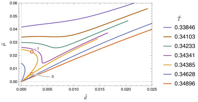
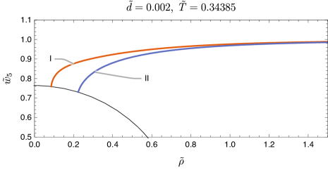
Figure 1: (top) Relation between the density and chemical potential for various temperatures. (bottom) Brane embeddings corresponding to I and II in the top-panel.

By solving eq. (13), we obtain relation between $\tilde{d}$ and $\tilde{\mu}$ for several $\tilde{T}$, as we show in the top-panel of figure 1. The results agree with those obtained in ref. [6]. In the range of $0.34341<\tilde{T}<0.34468$, $\tilde{\mu}$ becomes a multivalued function of $\tilde{d}$, and hence there are multiple solutions for given $\tilde{d}$ at $\tilde{T}$. In the bottom panel of figure 1, we show the corresponding embeddings labeled by I and II at $\tilde{d}=0.002$ and $\tilde{T}=0.34385$. We refer the upper solution and the lower solution in the bottom panel of figure 1 as BH-I and II embedding, respectively. The first order phase transition occur in such a case. The transition points are determined from the free energy or the Maxwell construction as we discuss in Appendix A. At $\tilde{T}=0.34341$, the system has the second order phase transition when $\tilde{d}=0.0039385$. At a temperature out of the above range, there is a crossover.

The phase structures are summarized as phase diagrams in figure 2. The phase structure changes depending on whether $\tilde{d}$ or $\tilde{\mu}$ is treated as a controlling parameter, in other words, considering a canonical ensemble or a grand canonical ensemble, respectively. We show the 1st order transition line as the black curve, and the 2nd order phase transition line as the black dashed line. In the canonical ensemble, the range of the phase transition are $0.34341<\tilde{T}<0.34468$ and $0<\tilde{d}<\tilde{d}_{c}=0.0039385$. In this case, the embeddings are always given by the BH embeddings but it is divided by the 1st order phase transition line in $\tilde{T}$ for $\tilde{d}<\tilde{d}_{c}$. We call the low- and high-temperature regime in $\tilde{d}<\tilde{d}_{c}$ as BH-I and BH-II phase, respectively. The BH-I and II embedding shown in the bottom panel of figure 1 belong to BH-I and II phase, respectively. In the grand canonical ensemble, there are brane solutions without touching the black hole horizon called Minkowski embeddings. The Minkowski embeddings realizes with vanishing density. We do not focus on such solutions in this study.

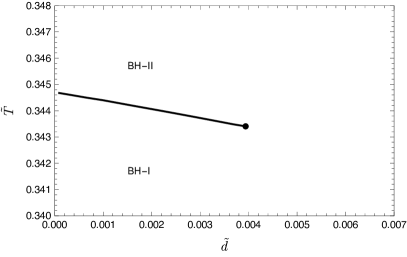
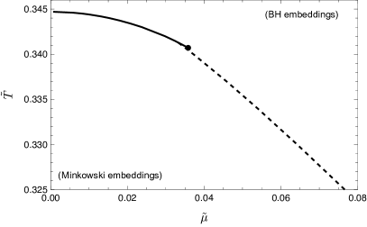
Figure 2: Phase diagrams of the probe brane. (left) Canonical ensemble, i.e., $\tilde{d}$ is a controlling parameter. The black line is the 1st order phase transition line. The endpoint at $\tilde{d}=\tilde{d}_{c}\approx 0.004$ indicates the 2nd order phase transition endpoint. For $\tilde{d}<\tilde{d}_{c}$, we call the low- and high-temperature regime as BH-I and BH-II phase, respectively. (right) Grand canonical ensemble, i.e., $\tilde{\mu}$ is a controlling parameter. The black line is the 1st order phase transition line. The dashed line denotes the 2nd order phase transition line.

3 Probing by a fermionic field

In this section, we consider dynamics of spinor field probing the background D7-brane’s worldvolume. As a first step of the study of the fermionic spectral function in the D3-D7 model, we consider the fermion’s action governed by the five dimensional part of the induced metric (7) ignoring the 3-sphere part of induced metric to avoid the technical complication. This should not change the essential features since the shape of the brane is already encoded in 5 dimensional model and extra factors of $\cos\theta$ in the measure should not change the qualitative features of the theory. We also present discussion of the other formulation and the problem arising there in Appendix B.

We now consider the following simplified model:

$$S_{\text{spinor}}=i\int\differential[5]{x}\sqrt{-\det h_{\mu\nu}}\bar{\psi}\left(\gamma^{\mu}\mathcal{D}_{\mu}-m\right)\psi+S_{\text{bou}},$$ (16)

where $h_{\mu\nu}$ is the five-dimensional part of the induced metric, that is,

$$h_{\mu\nu}\differential{x^{\mu}}\differential{x^{\nu}}=\frac{1}{u^{2}}\left[-\frac{f(u)^{2}}{\tilde{f}(u)}\differential{t}^{2}+\tilde{f}(u)\differential{x}^{2}\right]+\left(\frac{1}{u^{2}}+\theta^{\prime}(u)^{2}\right)\differential{u}^{2}.$$ (17)

$\mathcal{D}_{\mu}=\nabla_{\mu}-iqA_{\mu}$ is a gauge covariant derivative and $S_{\text{bdy}}$ is the boundary action which will be specified later. Notice that, the covariant derivative is also defined with respect to the 5 dimensional metric $h_{\mu\nu}$. Using the spin connection with respect to $h_{\mu\nu}$, it can be written as

$$\nabla_{\mu}=\partial_{\mu}+\frac{1}{8}\omega_{\mu}{}^{\underline{\nu\rho}}[\gamma_{\underline{\nu}},\gamma_{\underline{\rho}}],$$ (18)

where $\gamma^{\mu}$ denotes gamma matrices in the curved spacetime and $\gamma_{\underline{\mu}}$ are gamma matrices in the tangent space that will be defined as follows: It can be written as $\gamma^{\mu}=e^{\mu}{}_{\underline{\mu}}\gamma^{\underline{\mu}},$ where $e^{\mu}{}_{\underline{\mu}}$ is the inverse matrix of vielbein $e_{\mu}{}^{\underline{\mu}}$ which satisfies $e_{\mu}{}^{\underline{\mu}}e_{\nu}{}^{\underline{\nu}}\eta_{\underline{\mu\nu}}=h_{\mu\nu}$, and $\gamma^{\underline{\mu}}$ is the gamma matrices in the tangent space. The gamma matrices in the five-dimensional spacetime can be chosen as

$$\gamma^{\underline{0}}=\sigma^{1}\otimes i\sigma^{2},\quad\gamma^{\underline{1}}=\sigma^{1}\otimes\sigma^{1},\quad\gamma^{\underline{2}}=\sigma^{1}\otimes\sigma^{3},\quad\gamma^{\underline{3}}=\sigma^{2}\otimes I_{2},\quad\gamma^{\underline{u}}=\sigma^{3}\otimes I_{2},$$ (19)

where $\sigma^{1},\sigma^{2},\sigma^{3}$ are the Pauli matrices. Then, $\psi(x^{\mu})$ is written as a four-components spinor field.

The equation of motion is obtained as the following Dirac equation

$$\left(\gamma^{\mu}\mathcal{D}_{\mu}-m\right)\psi(t,\vec{x},u)=0.$$ (20)

Substituting the five dimensional metric, we can write

$$\gamma^{\mu}\mathcal{D}_{\mu}={e^{\nu}}_{\underline{\mu}}\gamma^{\underline{\mu}}(\partial_{\mu}-iqA_{\mu})+\frac{1}{4}{e^{u}}_{\underline{u}}\gamma^{\underline{u}}\partial_{u}\ln(-\det(h_{\mu\nu})h^{uu}).$$ (21)

Considering the following transformation

$$\psi(x^{\mu})=\left(-\det(h_{\mu\nu})h^{uu}\right)^{-1/4}\phi(x^{\mu}),$$ (22)

we obtain the following equation

$$\left[{e^{\nu}}_{\underline{\mu}}\gamma^{\bar{\mu}}(\partial_{\nu}-iqA_{\nu})-m\right]\phi(x^{\mu})=0.$$ (23)

We decompose the four-components spinor field $\psi$, as follows,

$$\psi(x^{\mu})=\psi_{+}(t,\vec{x},u)+\psi_{-}(t,\vec{x},u),$$ (24)

where $\psi_{\pm}$ are projected by $\psi_{\pm}=P_{\pm}\psi$ with $P_{\pm}=(1\pm\gamma^{u})/2$. According to ref. [15], the asymptotic behaviors of the spinors are written as

$$\psi_{+}=\psi_{+}^{(0)}u^{\Delta_{-}}+\psi_{+}^{(1)}u^{1+\Delta_{+}}+\cdots,\quad\psi_{-}=\psi_{-}^{(0)}u^{\Delta_{+}}+\psi_{-}^{(1)}u^{1+\Delta_{-}}\cdots,$$ (25)

where $\Delta_{\pm}=2\pm m$. $\psi_{\pm}^{(0)}$ and $\psi_{\pm}^{(1)}$ are related to the source and fermionic operator with the scaling dimension of $\Delta_{+}$, respectively. To obtain retarded responses, we also impose the ingoing-wave boundary condition at the black hole horizon. In order to compute the Green’s function, we need to fix the boundary action. We employ

$$S_{\text{bdy}}=\lim_{u\to\varepsilon}\frac{i}{2}\int\differential[4]x\sqrt{-hh^{uu}}\bar{\psi}\psi,$$ (26)

where $\varepsilon$ is a small positive cutoff $\varepsilon$, and $\bar{\psi}_{+}=\psi^{\dagger}\gamma^{0}$. This choice of the boundary term is known as the standard quantization [25]. The retarded Green’s function is obtained by

$$G^{\text{R}}(k)=i\mathcal{S}\gamma^{0}=\frac{2m+1}{k^{2}}(\gamma\cdot k)\mathcal{T}\gamma^{0},$$ (27)

where $\mathcal{S}$ and $\mathcal{T}$ are defined by

$$\psi_{-}^{(1)}=\mathcal{S}\psi_{+}^{(0)},\quad\psi_{+}^{(1)}=\mathcal{T}\psi_{-}^{(0)}.$$ (28)

The Green’s function has a scaling dimension of $-2m$. We can also derive the flow equation for $G^{\mathrm{R}}(k,u)$ from the Dirac equation, as those in ref. [19]. In the following section, we compute the result by solving the flow equation.

For later convenience, we define spectral function by

$$A(\omega,|\vec{k}|)=-\mathrm{Im}\tr G^{\mathrm{R}}(\omega,\vec{k}).$$ (29)

Since the system is isotropic, $A(\omega,k)$ depends only on $k\equiv|\vec{k}|$. We also define a scaled spectral function

$$\tilde{A}(\tilde{\omega},\tilde{k})=m_{q}^{2m}\times A(m_{q}\tilde{\omega},m_{q}\tilde{k}).$$ (30)

3.1 Spectral function

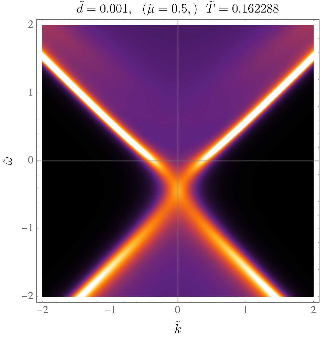
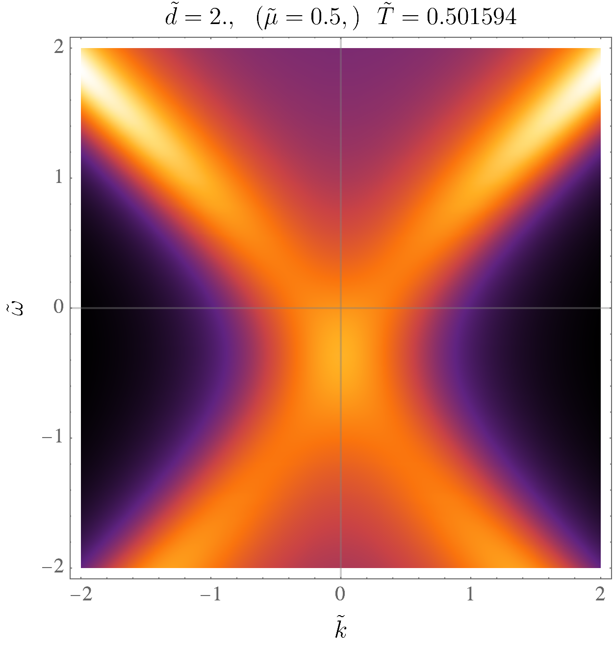
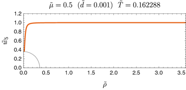
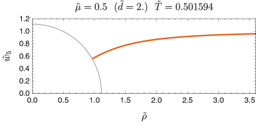
Figure 3: (top) Spectral functions $\tilde{A}(\tilde{\omega},\tilde{k})$ for two setups. We set $m=0.2$. (bottom) Brane embeddings corresponding to the top panels, respectively. The black circle shows the location of the black hole horizon.

We show the spectral functions of the two embeddings with $\tilde{\mu}=0.5$ in figure 3. The left panel of figure 3 corresponds to a solution in the BH-I phase, and the right panel of figure 3 corresponds to a solution in the crossover region in figure 2. The spectral function of the left panel of figure 3 is similar to those obtained in ref. [26]. In both cases, the Dirac points are shifted by $\mu$. It is also similar to the results of refs. [13, 26]. As $T$ increases, the peaks of the spectral function are smeared.

It is considered that the Fermi level is located at $\omega=0$. The intersection between the peaks and the horizontal axis is considered as the Fermi surface but it is smeared at finite temperatures. In the following, we define the Fermi momentum of the smeared Fermi surface, and the width of the Drude-like peak.

3.2 Smeared Fermi surface

At finite temperatures the Fermi surface is smeared, so we can no longer define sharp Fermi momentum $k_{F}$. However, we can still define an analogous of $k_{F}$ from the ’pole’ of the retarded Green’s function there. In normal isotropic metals, $k_{F}$ satisfies $E(k_{F})=\mu$ where $E(k)$ denotes the dispersion relation. The spectral function should have a delta function peak at the Fermi momentum:

$$A(\omega=0,\vec{k})\propto\delta(k-k_{F}).$$ (31)

We have assumed $\omega=0$ is the Fermi level. It implies that the Green’s function has a pole structure of

$$\mathrm{tr}G^{\mathrm{R}}(\omega,k)=\frac{Z}{\omega-k+k_{F}+i0_{+}}+\cdots,$$ (32)

where $Z$ is a constant, and the ellipsis denotes contributions from the other poles and the regular part.

At finite temperatures, the spectral function is smeared. The pole, then, must be located on the lower half complex $\omega$-plane with a finite distance from the real axis. We assume the pole structure of the Green’s function as

$$\tr G^{\mathrm{R}}(\omega,k)=\frac{Z_{\Gamma}}{\omega-k+k_{F}^{\prime}+i\Gamma/2}+\cdots,$$ (33)

where $\Gamma$ is the width, i.e., the decay constant. $Z_{\Gamma}$ is a constant residue. $k_{F}^{\prime}$ is also a positive real constant which can be understood as a center of smeared Fermi momentum. Taking the inverse of $\tr G^{\mathrm{R}}$ and evaluating it at $(\omega,k_{F})=(-i\Gamma/2,k_{F}^{\prime})$, we obtain the equation

$$\frac{1}{\tr G^{\mathrm{R}}(\omega=-i\Gamma/2,k=k_{F}^{\prime})}=0.$$ (34)

We can determine $k_{F}^{\prime}$ and $\Gamma$ by solving this complex valued equation. In the following, we will study the behavior of $\Gamma$ by using eq. (34).

3.3 $T$-dependence of the decay rate

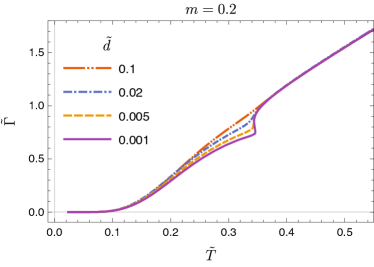
(a) D3-D7

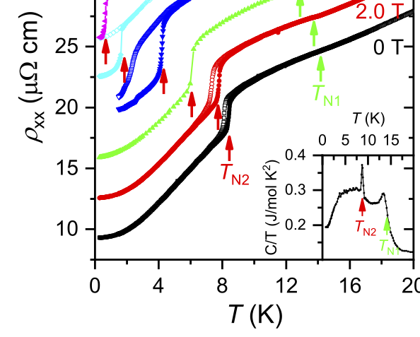
(b) experimental data

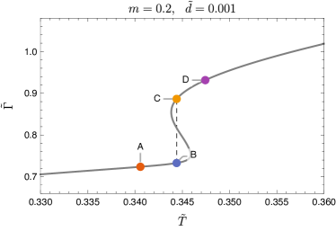
(c) Width $\tilde{\Gamma}$ vs temperature $\tilde{T}$ for $\tilde{d}=0.001$.

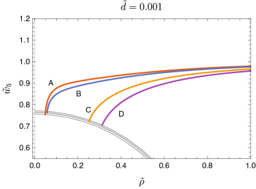
(d) Probe-brane’s embeddings

Figure 4: (a)${\Gamma}$ vs ${T}$ for various ${densities}$. Low density shows first order transition. (b) The black line is the experimental data with vanishing magnetic fields $B=0$ to be compared with figure(a). In (c), the vertical dashed line denotes the critical temperature where the first order phase transition occurs. The points labeled by A to D correspond to the embeddings in the right panel, respectively. In (d), the gray circles denote the black hole horizon at each temperatures. The embeddings B and C have a common temperature $\tilde{T}=\tilde{T}_{c}$. The figure(b) is from [27].

From eq. (34), we compute $\Gamma$ for various temperatures. We define the scaled width by $\tilde{\Gamma}\equiv\Gamma/m_{q}$. Figure 4 shows the width ${\Gamma}$ as functions of the temperature ${T}$ for various values of scaled density and chemical potential, $\tilde{d}$ and $\tilde{\mu}$. In both cases, we find that ${\Gamma}$ is linear in ${T}$ at high temperatures. For sufficiently low density, the curves have small multivalued region around ${T}=0.35m_{q}$ corresponding to the multivalued results shown in figure 1(a). When ${T}$ is taken to sufficiently small, ${\Gamma}$ depends on ${T}$ as ${\Gamma}\approx\gamma e^{-\alpha/{T}}$ with a positive constant $\alpha$ near zero temperature. These behaviors along the temperature may appear in various holographic models, e.g., see ref. [17].

The figure 4(c) shows an enlarged view of figure 4(a) around the phase transition point for $\tilde{d}=0.001$. The dotted vertical dashed line shows the transition point at $T=T_{c}=0.34440$. In adiabatic measurements, it is anticipated that the results will exhibit a discontinuity between points B and C, with the intermediate S-shaped branch being omitted. We show the brane embeddings for the points labeled by A to D in figure 4(d). The points A, B belong to the BH-I phase, and C, D belong to the BH-II phase.

We point out that our result showing the first order transition from a black hole phase to another black hole phase exhibits a qualitative similarity to the experimental measurement of the resistivity in an anti-ferromagnetic Kondo compound [28, 27] some of which is captured in figure 4(b) showing the experimental result of ref. [27]. The Kondo compound also exhibit a drop of the first order phase transition in the resistivity and the data certainly suggests that there is a first order phase transition from a strange metal to another strange metal with different slope although at the present time the microscopic reason for such transition is not known.

We have to make a few remarks: First, our model of the probe fermion is a simplified model where extra dimension of 3 sphere is neglected. The treatment of the extra-dimensions in the brane should be improved in the future. Second, our result (figure 4(a)) is plotted for the width but the experimental result (figure 4(b)) is for the resistivity. In the Drude picture, the resistivity is proportional to the Drude width. In our model, the resistivity (or conductivity) computed by the well-known method, e.g., the membrane paradigm, does not agree with the behavior of the width. This feature of the transport is actually common to all holographic model: while the resistivity linear in $T$ is universal for all strange metal with strong correlation, the holographic calculation shows such behavior comes only for some fine tuned model in extreme low temperature phase, which is not the property of the strange metals. Perhaps the present understanding of holographic calculation of the conductivity involves some conceptual misunderstanding. This is a serious and challenging problem to the holography. We follow the point of ref. [17] where it was pointed out that instead of relying on the standard scheme of calculating conductivity, if we assume the Drude picture even in the case of the strange metal, then we can understand the universality of the strange metal. In fact, this is the assumption of all SYK model also as well as in the discussion of the so called ‘plankian dissipation’. We hope that our finding of similarity of the dropping in fermion width and that of transport shed some light on this matter.

4 Discussions

In this paper, we study the fermionic spectral function in the D3-D7 model by considering the toy model of the probe spinor field. From the spectral function, we investigate the behavior of the width for varying the temperature. We find that the width also shows the dropping behavior corresponding to the first order phase transition between the BH-I and BH-II phase. We mentioned the transport data related to the fermion spectral function based on the Drude model. It is partially related to the puzzle in the holography: while the transport coefficients calculated with holographic method are too sensitive to the details of the background, those in the metallic phase of real condensed matter with strong correlations are universal which exhibit the linear in $T$ resistivity. At this moment, it is not clear what is missing point in the general method of the holographic calculation of the transport. Therefore, in the meantime, we should find a bypass track like the method we adopted: use the fermion width with the Drude picture. For some reasons, the fermion width is shown to be universal.[19] We also point out, as shown in figure 4, the similarity between our result and the experimental result of the resistivity in some kinds of Kondo compound [28, 27].

The first order phase transition is one of the characteristic behaviors in the brane models. While the holographic superconductors exhibit only the second order phase transition, the brane models often show the first order phase transition. One of the our motivation was to understand the physical meaning of the first order phase transition between the two black hole phases using the probe fermion. Indeed, in the measurement of the Kondo compounds [28, 27], such a feature was observed in the temperature dependence of the resistivity as shown in section 3. We found the similar behavior in the width of the fermionic spectral function in our model. We expect that there is a common mechanism existing for the first order transition between two dissipative phases both in the D3-D7 model and those Kondo compounds. As far as we know, the physical meaning of the low temperature phase and the first order phase transition is still not understood even in the context of the Kondo compounds. It would be very interesting if we can reveal the above point by further investigation.

Appendix A The free energy and phase transition points

In this section, we discuss the free energy of the probe brane and the phase transitions. The phase transition points can be determined from the thermodynamics of the probe brane. We interpret the on-shell action of eq. (12) as a Helmholtz free energy [6]:

$$F_{0}(d)=\int_{u_{h}}^{\epsilon}\tilde{\mathcal{L}}(d)\differential{u}$$ (35)

Since this integral is still divergent, we have to regularize it. According to [29] which is equivalent to the procedure in [5, 6], the counterterms are given by

$$L_{1}=\frac{1}{4}\mathcal{N}\sqrt{-\gamma},\quad L_{2}=-\frac{1}{2}\mathcal{N}\sqrt{-\gamma}\theta(\epsilon)^{2},\quad L_{f}=\mathcal{N}\frac{5}{12}\sqrt{-\gamma}\theta(\epsilon)^{4},$$ (36)

where $\gamma$ is the induced metric at $z=\epsilon$ near the AdS boundary and $\sqrt{-\gamma}=\epsilon^{-4}$. Substituting $\theta(u)=\theta_{0}u+\theta_{2}u^{2}+\cdots$, we obtain

$$L_{1}=\frac{\mathcal{N}}{4}\frac{1}{\epsilon^{4}},\quad L_{2}=-\mathcal{N}\left(\frac{1}{2}\frac{\theta_{0}^{2}}{\epsilon^{2}}+\theta_{0}\theta_{2}\right),\quad L_{f}=\mathcal{N}\frac{5}{12}\theta_{0}^{4}.$$ (37)

The coefficients $\theta_{0}$ and $\theta_{2}$ are related to the quark mass $m_{q}$ and the quark condensate $c$ by

$$\theta_{0}=m_{q},\quad\theta_{2}=c+\frac{1}{6}m_{q}^{3},$$ (38)

respectively. We write

$$L_{ct}= L_{1}+L_{2}+L_{f}=\mathcal{N}\left[\frac{1}{4\epsilon^{4}}-\frac{m_{q}^{2}}{2\epsilon^{2}}-m_{q}\left(c+\frac{1}{6}m_{q}^{3}\right)+\frac{5}{12}m_{q}^{4}\right]$$ (39)

$$= \mathcal{N}\int_{u_{h}}^{\epsilon}\left[-\frac{1}{u^{5}}+\frac{m_{q}^{2}}{u^{3}}\right]\differential{u}+\mathcal{N}\left(\frac{1}{4u_{h}^{4}}-\frac{m_{q}^{2}}{2u_{h}^{2}}\right)+\mathcal{N}\left(\frac{m_{q}^{4}}{4}-m_{q}c\right).$$

Then, the regularized free energy can be computed by

$$F=\int_{u_{h}}^{\epsilon}\tilde{\mathcal{L}}\differential{u}+L_{ct}=\int_{u_{h}}^{\epsilon}\left[\tilde{\mathcal{L}}+\mathcal{N}\left(-\frac{1}{u^{5}}+\frac{m_{q}^{2}}{u^{3}}\right)\right]\differential{u}+\mathcal{N}\left(\frac{1}{4u_{h}^{4}}-\frac{m_{q}^{2}}{2u_{h}^{2}}+\frac{m_{q}^{4}}{4}-m_{q}c\right).$$ (40)

In the multivalued region, $F(d)$ has swallowtail structure as a function of $d$, as shown in figure 5. In such cases, the intersection of the two branch of $F(d)$ is considered as a phase transition point.

The free energy is a thermodynamic potential in the grand canonical ensemble. In this case, $d$ is treated as a controlling parameter. On the other hand, we can also consider the canonical ensemble setup when we treat $\mu$ as a controlling parameter. In the canonical ensemble, the thermodynamic potential is given by the grand potential

$$\Omega(\mu)=F-\mu d.$$ (41)

Figure 6 shows $\Omega/T^{4}$ as a function of $\tilde{\mu}$ at $\tilde{T}=0.343737$. Note that there is the branch of the Minkowski embedding with vanishing density but finite $\mu$. Considering both of the Minkowski and BH embeddings, we can find swallowtail structure in $\Omega(\mu)$. The intersection point of the swallowtail in $\Omega(\mu)$ is the 1st order phase transition point. At low temperatures, the multivalued region of $\tilde{d}$ as a function of $\tilde{\mu}$ disappears. Then, $\tilde{d}$ goes zero at finite $\tilde{\mu}$ without the multivaluedness. It means the 2nd order phase transition from the BH embedding to the Minkowski embedding.

The phase diagrams of the grand canonical and the canonical ensemble setups are shown in figure 2.

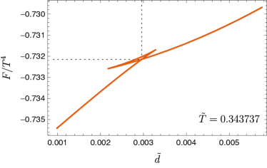
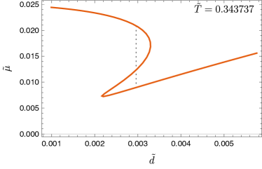
Figure 5: (left) Free energy vs density at $\tilde{T}=0.343737$. The dotted lines shows the 1st order phase transition point at $\tilde{d}\approx 0.003$. (right) $\tilde{\mu}$ vs $\tilde{d}$. The vertical dotted line shows the phase transition point.

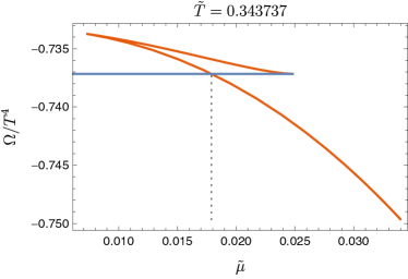
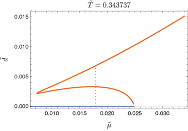
Figure 6: (left) Grand potential vs chemical potential at $\tilde{T}=0.343737$. The dotted line shows the 1st order phase transition point at $\tilde{\mu}\approx 0.018$. The red and blue curve show results in the BH and the Minkowski embedding, respectively. (right) $\tilde{d}$ vs $\tilde{\mu}$. The vertical dotted line shows the phase transition point.

Appendix B A fermionic field living in the worldvolume

In this section, we consider a fermionic field living in the eight dimensional worldvolume of the D7-brane. In this formulation, we encounter the problem of the unitary bound for the fermionic operator.

The model is

$$S_{\text{spinor}}^{\prime}=i\int\differential[8]{\xi}\sqrt{-\det h_{ab}}\bar{\Psi}\Gamma^{a}D_{a}\Psi+S_{\text{bdy}}^{\prime},$$ (42)

where $h_{ab}$ denotes the 8-dimensional induced metric of the D7-brane’s worldvolume (7), $S_{bdy}^{\prime}$ is a boundary term. For simplicity, we consider no mass term for the eight dimensional theory. The gauge covariant derivative is given by

$$D_{a}=\nabla_{a}-iqA_{a}=\partial_{a}+\frac{1}{4}\omega_{a}{}^{\alpha\beta}\Gamma_{\alpha\beta}-iqA_{a},$$ (43)

where $q$ is a charge of the fermionic field, and we will set $q=1$ in this study. $\alpha,\beta$ denote indices for the locally flat coordinates of the worldvolume coordinates. $\omega_{a}{}^{\alpha\beta}$ is a spin connection of $h_{ab}$. $\Gamma^{\alpha}$ are gamma matrices, and $\Gamma^{a}$ are also defined by $\Gamma^{a}={e^{a}}_{\alpha}\Gamma^{\alpha}$ with the inverse of the vielbeins ${e^{a}}_{\alpha}$ satisfying ${e^{a}}_{\alpha}{e^{b}}_{\beta}\eta^{\alpha\beta}=h^{ab}$. $\Gamma^{\alpha_{1}\alpha_{2}\cdots\alpha_{p}}$ are defined by $\Gamma^{\alpha_{1}\alpha_{2}\cdots\alpha_{p}}=\Gamma^{[\alpha_{1}}\Gamma^{\alpha_{2}}\cdots\Gamma^{\alpha_{p}]},$ for $1<p\leq 8$. The field equation derived by the action is the following 8 dimensional Dirac equation

$$\Gamma^{a}D_{a}\Psi=0.$$ (44)

Here, we need to consider the Clifford algebra in the 8 dimensional worldvolume of the D7-brane. The dimension of the irreducible representation of the Clifford algebra is given by $2^{\lfloor D/2\rfloor}$ for a spacetime dimension $D$, and hence we need $2^{8/2}=16$ dimensional representation of the gamma matrices. According to Ref. [23], we choose the 8 dimensional gamma matrices as

$$\Gamma^{\underline{\mu}}=I_{2}\otimes\sigma^{1}\otimes\gamma^{\mu},\quad\Gamma^{\underline{i}}=\gamma^{i}\otimes\sigma^{2}\otimes I_{4},$$ (45)

where $\mu,\nu$ denotes $0,1,2,3,u$ and $i,j$ are for 3-sphere coordinates, and $\sigma^{1},\sigma^{2},\sigma^{3}$ are the Pauli matrices. We emphasized that it is component in the tangent space by the notation of $\Gamma^{\underline{\alpha}}=\Gamma^{\alpha}$. We need 4 and 2 dimensional representation for the AdS₅ part and 3-sphere part of the gamma matrices, respectively. $\gamma^{\mu}$ and $\gamma^{i}$ satisfy

$$\anticommutator{\gamma^{\mu}}{\gamma^{\nu}}=2\eta^{\mu\nu},\quad\anticommutator{\gamma^{i}}{\gamma^{j}}=2\delta^{ij},$$ (46)

then $\Gamma^{\alpha}$ also satisfy the Clifford algebra $\anticommutator{\Gamma^{\alpha}}{\Gamma^{\beta}}=2\eta^{\alpha\beta}$. We choose $\gamma^{\mu}$ as (19) and $\gamma^{i}=\sigma^{i}$ for 3-sphere part.

Now, we employ the following ansatz

$$\Psi(x^{\mu})=\chi(\Omega_{3})\otimes\zeta\otimes\psi(x^{\mu}),$$ (47)

where $\chi$ is a two-component spinor field of the 3 sphere, $\zeta$ is a constant two-component spinor and $\psi$ is a four-component spinor field of the AdS₅-part. By using the metric (7), we can write the covariant Dirac operator as

$$\Gamma^{a}\nabla_{a}=\Gamma^{\mu}\partial_{\mu}+\frac{1}{4}{e^{u}}_{\underline{u}}\Gamma^{\underline{u}}\partial_{u}\ln(-\det\hat{h}h^{uu})+\Gamma^{i}\nabla_{i},$$ (48)

where the second term comes from the spin connection term, and $\det\hat{h}\equiv\det h/\det g_{\mathrm{S}^{3}}$ with a metric of the unit 3 sphere $g_{\mathrm{S}^{3}}$. The last term is a covariant derivative for the 3-sphere part. Note that $\det\hat{h}$ does not depend on the 3-sphere coordinates. The kinetic term of the Dirac equation becomes

$$\Gamma^{a}D_{a}\Psi=\chi\otimes\sigma^{1}\zeta\otimes\not{\mathcal{D}}\psi+\frac{1}{\cos\theta}\not{\nabla}_{\mathrm{S}^{3}}\chi\otimes\sigma^{2}\zeta\otimes\psi,$$ (49)

where

$$\not{\mathcal{D}}={e^{\nu}}_{\underline{\mu}}\gamma^{\mu}(\partial_{\mu}-iqA_{\mu})+\frac{1}{4}{e^{u}}_{\underline{u}}\gamma^{u}\partial_{u}\ln(-\det\hat{h}h^{uu}),$$ (50)

and $\not{\nabla}_{\mathrm{S}^{3}}$ is a covariant Dirac operator in the unit 3 sphere. $\chi(\Omega_{3})$ should be set to the eigenspinors $\chi_{l}^{\pm}$ in the unit 3 sphere satisfying

$$\not{\nabla}_{\mathrm{S}^{3}}\chi_{l}^{\pm}=i\alpha_{l}^{\pm}\chi_{l}^{\pm},$$ (51)

where $\alpha_{l}^{\pm}=\pm(l+3/2)$ [30]. It is orthonormalized by

$$\int_{\mathrm{S}^{3}}\mathrm{vol}(\mathrm{S}^{3})(\chi^{s}_{l})^{\dagger}\chi^{s^{\prime}}_{l^{\prime}}=\delta_{ss^{\prime}}\delta_{ll^{\prime}},$$ (52)

where $\mathrm{vol}(\mathrm{S}^{3})$ is a volume form of the unit 3 sphere. In the boundary theory, $l$ is interpreted as a quantum number of the isospin charge.

The Dirac equation becomes

$$\chi_{l}^{\pm}\otimes\left[\sigma^{1}\zeta\otimes\not{\mathcal{D}}\psi+i\sigma^{2}\zeta\otimes\frac{\alpha_{l}^{\pm}}{\cos\theta}\psi\right]=0.$$ (53)

Now, we set $\zeta=\zeta_{\uparrow}$ which satisfy $\sigma^{1}\zeta_{\uparrow}=\zeta_{\downarrow}$ and $\sigma^{2}\zeta_{\uparrow}=-i\zeta_{\downarrow}$ where $\zeta_{\uparrow}=(1,0)^{T}$ and $\zeta_{\downarrow}=(0,1)^{T}$. Dropping the extra extra-dimensional part of the spinor, we obtain the five-dimensional Dirac equation as

$$\left[\not{\mathcal{D}}+\frac{\alpha_{l}^{\pm}}{\cos\theta}\right]\psi=0.$$ (54)

Since $\cos\theta(u)=1$ at $u=0$, $m_{l}=-\alpha_{l}^{\pm}$ can be read as a five-dimensional bulk mass of the $\psi$. It is related with the scaling dimension of fermionic operator by

$$\Delta_{\pm}^{l}=\frac{d}{2}\pm m_{l}=2\pm\left(l+\frac{3}{2}\right),$$ (55)

where $d=4$ in our case. On the other hand, the scaling dimension of the fermionic operator is restricted by the unitary bound. It was pointed out that the violation of the unitary bound of the fermionic operator leads instability by ref. [31]. To ensure the unitary bound, the bulk mass of the fermionic field must satisfies $|m|\leq 1/2$. In the current case, however, the smallest absolute mass is $|m_{0}|=3/2$ which violates the unitary bound. This bulk mass is Kaluza-Klein mass arising from the compactification in $S^{3}$. It naturally arises and cannot be ignored if we begin from the theory with a ten dimensional spacetime. In the case of the mesino fluctuations, there is also another mass contribution in the top-down fermionic action. The bulk mass of the mesino fluctuation for each top-down model were summarized as table 1 in ref. [22]. The violation of the unitary bound might be cured by the presence of the finite isospin charge. We leave the above problem as an open question.

References

- [1] J. M. Maldacena, “The Large N limit of superconformal field theories and supergravity,” Adv. Theor. Math. Phys. 2 (1998) 231–252, arXiv:hep-th/9711200.
- [2] S. S. Gubser, I. R. Klebanov, and A. M. Polyakov, “Gauge theory correlators from noncritical string theory,” Phys. Lett. B 428 (1998) 105–114, arXiv:hep-th/9802109.
- [3] E. Witten, “Anti-de Sitter space, thermal phase transition, and confinement in gauge theories,” Adv. Theor. Math. Phys. 2 (1998) 505–532, arXiv:hep-th/9803131.
- [4] A. Karch and E. Katz, “Adding flavor to AdS / CFT,” JHEP 06 (2002) 043, arXiv:hep-th/0205236.
- [5] S. Nakamura, Y. Seo, S.-J. Sin, and K. P. Yogendran, “A New Phase at Finite Quark Density from AdS/CFT,” J. Korean Phys. Soc. 52 (2008) 1734–1739, arXiv:hep-th/0611021.
- [6] S. Nakamura, Y. Seo, S.-J. Sin, and K. P. Yogendran, “Baryon-charge Chemical Potential in AdS/CFT,” Prog. Theor. Phys. 120 (2008) 51–76, arXiv:0708.2818 [hep-th].
- [7] D. Mateos, R. C. Myers, and R. M. Thomson, “Holographic phase transitions with fundamental matter,” Phys. Rev. Lett. 97 (2006) 091601, arXiv:hep-th/0605046.
- [8] D. Mateos, R. C. Myers, and R. M. Thomson, “Thermodynamics of the brane,” JHEP 05 (2007) 067, arXiv:hep-th/0701132.
- [9] M. Kruczenski, D. Mateos, R. C. Myers, and D. J. Winters, “Meson spectroscopy in AdS / CFT with flavor,” JHEP 07 (2003) 049, arXiv:hep-th/0304032.
- [10] J. Erdmenger, M. Kaminski, and F. Rust, “Holographic vector mesons from spectral functions at finite baryon or isospin density,” Phys. Rev. D 77 (2008) 046005, arXiv:0710.0334 [hep-th].
- [11] R. C. Myers, A. O. Starinets, and R. M. Thomson, “Holographic spectral functions and diffusion constants for fundamental matter,” JHEP 11 (2007) 091, arXiv:0706.0162 [hep-th].
- [12] J. Mas, J. P. Shock, J. Tarrio, and D. Zoakos, “Holographic Spectral Functions at Finite Baryon Density,” JHEP 09 (2008) 009, arXiv:0805.2601 [hep-th].
- [13] H. Liu, J. McGreevy, and D. Vegh, “Non-Fermi liquids from holography,” Phys. Rev. D 83 (2011) 065029, arXiv:0903.2477 [hep-th].
- [14] T. Faulkner, H. Liu, J. McGreevy, and D. Vegh, “Emergent quantum criticality, Fermi surfaces, and AdS(2),” Phys. Rev. D 83 (2011) 125002, arXiv:0907.2694 [hep-th].
- [15] N. Iqbal and H. Liu, “Real-time response in AdS/CFT with application to spinors,” Fortsch. Phys. 57 (2009) 367–384, arXiv:0903.2596 [hep-th].
- [16] T. Faulkner, G. T. Horowitz, J. McGreevy, M. M. Roberts, and D. Vegh, “Photoemission ’experiments’ on holographic superconductors,” JHEP 03 (2010) 121, arXiv:0911.3402 [hep-th].
- [17] E. Oh, T. Yuk, and S.-J. Sin, “The emergence of strange metal and topological liquid near quantum critical point in a solvable model,” JHEP 11 (2021) 207, arXiv:2103.08166 [hep-th].
- [18] E. Oh, Y. Seo, T. Yuk, and S.-J. Sin, “Ginzberg-Landau-Wilson theory for Flat band, Fermi-arc and surface states of strongly correlated systems,” JHEP 01 (2021) 053, arXiv:2007.12188 [hep-th].
- [19] T. Yuk and S.-J. Sin, “Flow equation and fermion gap in the holographic superconductors,” JHEP 02 (2023) 121, arXiv:2208.03132 [hep-th].
- [20] L. Martucci, J. Rosseel, D. Van den Bleeken, and A. Van Proeyen, “Dirac actions for D-branes on backgrounds with fluxes,” Class. Quant. Grav. 22 (2005) 2745–2764, arXiv:hep-th/0504041.
- [21] I. Kirsch, “Spectroscopy of fermionic operators in AdS/CFT,” JHEP 09 (2006) 052, arXiv:hep-th/0607205.
- [22] M. Ammon, J. Erdmenger, M. Kaminski, and A. O’Bannon, “Fermionic Operator Mixing in Holographic p-wave Superfluids,” JHEP 05 (2010) 053, arXiv:1003.1134 [hep-th].
- [23] R. Abt, J. Erdmenger, N. Evans, and K. S. Rigatos, “Light composite fermions from holography,” JHEP 11 (2019) 160, arXiv:1907.09489 [hep-th].
- [24] A. Karch and A. O’Bannon, “Holographic thermodynamics at finite baryon density: Some exact results,” JHEP 11 (2007) 074, arXiv:0709.0570 [hep-th].
- [25] J. N. Laia and D. Tong, “A Holographic Flat Band,” JHEP 11 (2011) 125, arXiv:1108.1381 [hep-th].
- [26] M. Cubrovic, J. Zaanen, and K. Schalm, “String Theory, Quantum Phase Transitions and the Emergent Fermi-Liquid,” Science 325 (2009) 439–444, arXiv:0904.1993 [hep-th].
- [27] H. Wang, T. B. Park, S. Shin, H. Jang, E. D. Bauer, and T. Park, “Field-induced multiple quantum phase transitions in the antiferromagnetic kondo-lattice compound ,” Phys. Rev. B 105 (Apr, 2022) 165110. https://link.aps.org/doi/10.1103/PhysRevB.105.165110.
- [28] A. Maurya, R. Kulkarni, A. Thamizhavel, D. Paudyal, and S. K. Dhar, “Kondo lattice and antiferromagnetic behavior in quaternary cetal4si2 (t = rh, ir) single crystals,” Journal of the Physical Society of Japan 85 no. 3, (Mar, 2016) 034720. https://doi.org/10.7566%2Fjpsj.85.034720.
- [29] A. Karch, A. O’Bannon, and K. Skenderis, “Holographic renormalization of probe D-branes in AdS/CFT,” JHEP 04 (2006) 015, arXiv:hep-th/0512125.
- [30] R. Camporesi and A. Higuchi, “On the Eigen functions of the Dirac operator on spheres and real hyperbolic spaces,” J. Geom. Phys. 20 (1996) 1–18, arXiv:gr-qc/9505009.
- [31] G. Song, Y. Seo, and S.-J. Sin, “Unitarity bound violation in holography and the Instability toward the Charge Density Wave,” Int. J. Mod. Phys. A 35 no. 22, (2020) 2050128, arXiv:1810.03312 [hep-th].