Streaming Probabilistic PCA for Missing Data with Heteroscedastic Noise

Abstract

Streaming principal component analysis (PCA) is an integral tool in large-scale machine learning for rapidly estimating low-dimensional subspaces of very high dimensional and high arrival-rate data with missing entries and corrupting noise. However, modern trends increasingly combine data from a variety of sources, meaning they may exhibit heterogeneous quality across samples. Since standard streaming PCA algorithms do not account for non-uniform noise, their subspace estimates can quickly degrade. On the other hand, the recently proposed Heteroscedastic Probabilistic PCA Technique (HePPCAT) addresses this heterogeneity, but it was not designed to handle missing entries and streaming data, nor does it adapt to non-stationary behavior in time series data. This paper proposes the Streaming HeteroscedASTic Algorithm for PCA (SHASTA-PCA) to bridge this divide. SHASTA-PCA employs a stochastic alternating expectation maximization approach that jointly learns the low-rank latent factors and the unknown noise variances from streaming data that may have missing entries and heteroscedastic noise, all while maintaining a low memory and computational footprint. Numerical experiments validate the superior subspace estimation of our method compared to state-of-the-art streaming PCA algorithms in the heteroscedastic setting. Finally, we illustrate SHASTA-PCA applied to highly-heterogeneous real data from astronomy.

1 Introduction

Modern data are increasingly large in scale and formed by combining heterogeneous samples from diverse sources or conditions and exhibit heteroscedastic noise, or noises of different variances [1]. For example, in environmental monitoring, data from a few high precision instruments may be combined with a large volume of crowd-sourced data [1], and in astronomy, quasar spectra vary widely in quality across samples [2]. Recent advances in machine learning also consider data of heterogeneous quality, where data from different sources of varying quality are combined to leverage additional training samples. Many examples of this occur in settings like medical imaging; MRI coils exhibit varying signal-to-noise ratios [3], and computed tomography images vary in quality by radiation dose [4].

Principal component analysis (PCA) for visualization, exploratory data analysis, data compression, predictive tasks, or other downstream tasks is one of the most fundamental tools in machine learning. Well-studied and computable via a singular value decomposition or eigendecomposition, PCA requires a fully observed batch of data to estimate the batch’s principal components. However, in many applications, due to memory or physical constraints, the full data cannot be observed in its entirety at computation time and is instead read partially into memory piece by piece, or observations may stream in continuously and indefinitely. Likewise, the signal may evolve in time and require adaptive tracking algorithms for the low-rank component. Adding to these difficulties, it is also common for big data to contain missing entries. Magnetic resonance imaging (MRI) scans may subsample spatial frequencies [5], most user ratings of titles in collaborative filtering datasets are unobserved [6], and environmental sensing readings may occasionally drop out [7]. Consequently, there is a need for PCA techniques that can handle heteroscedastic noise, missing data, and scalability issues.

A tremendous body of work has studied streaming PCA techniques for learning a signal subspace from noisy incremental data observations with missing entries. Streaming or online PCA algorithms often enjoy the advantages of computational efficiency, low memory overhead, and adaptive tracking abilities, making them very useful in real world big-data applications. However, no existing streaming methods account for noise with different variances across samples, i.e., samplewise heteroscedastic noise, and their estimates can be highly corrupted by the noisiest samples. The work in [1] developed a Heteroscedastic Probabilistic PCA technique (HePPCAT) for data with varying noise levels across samples. HePPCAT learns the low-rank factors and the unknown noise variances via maximum likelihood estimation, but only in the batch setting with fully observed entries. Other batch heteroscedastic PCA algorithms liked weighted PCA studied in [8, 9, 10] and HeteroPCA [11] for data with heteroscedastic features also lack streaming and adaptive tracking abilities.

To the best of our knowledge, the present paper is the first work to develop a streaming PCA algorithm for heteroscedastic data with missing entries. Our algorithm estimates the factors and unknown noise variances in an online fashion from streaming incomplete data by using an efficient stochastic alternating minorize-maximize (MM) approach with small computational and memory overhead; the proposed method has close connections to the streaming PCA algorithm PETRELS [12]. We demonstrate that our algorithm can achieve superior estimation of the signal subspace (without knowledge of the noise variances) from subsampled data compared to state-of-the-art streaming PCA methods that assume homogeneous noise. Our algorithm can track not only dynamic low-dimensional subspaces, but also dynamic noise variances that occur in applications related to sensor calibration [13].

Section 2 discusses related works for both streaming PCA and heteteroscedastic PCA. Section 3 describes the model we consider, the resulting optimization problem, and the proposed algorithm. Section 7 presents synthetic and real data experiments that demonstrate the benefits of the proposed method over existing state-of-the-art streaming PCA algorithms.

1.1 Notation

We use bold upper case letters $\bm{A}$ to denote matrices, bold lower case letters $\bm{v}$ to denote vectors, and non-bold lower case letters $c$ for scalars. We denote the Hermitian transpose of a matrix as $\bm{A}^{\prime}$ and the trace of a matrix as $\operatorname{tr}(\bm{A})$. The Euclidean norm is denoted by $\|\cdot\|_{2}$. The identity matrix of size $d$ is denoted as $\bm{I}_{d}$. The notation $i\in[k]$ means $i=1,\dots,k$.

2 Related work

2.1 Streaming PCA

A rich body of work has developed and investigated a variety of streaming PCA algorithms for learning a signal subspace from incremental and possibly incomplete data observations. Each of these methods, however, assumes the data have homogeneous quality and do not model heteroscedastic properties like those considered in this paper. Since there are too many related works to detail here (see, e.g., [14], for a recent survey), we will highlight a few of the most related.

One prominent branch of algorithms utilizes stochastic gradient optimization approaches to update the learned subspace based on a new data observation at each iteration; see, e.g., [15, 16]. Mardani et al. [17] use stochastic gradient descent to learn matrix and tensor factorization models in the presence of missing data and also include an exponentially weighted data term that trades off adapting to new data with fitting historical data. Stochastic gradient descent over Riemannian manifolds is also a popular approach; see, e.g., [18, 19, 20, 21]. Oja’s method [22] takes a stochastic gradient step to update the subspace basis from the most recent data vector, obtaining a new orthonormal basis after orthogonalization. Recently, AdaOja introduced a way to adaptively select the learning rate to learn the subspace in one pass over the data [23]. Some streaming PCA methods share commonalities with quasi-second order optimization methods. For example, the PETRELS algorithm proposed in [12] fits a factor model to data with missing entries via a stochastic quasi-Newton method. PETRELS has computationally efficient updates but can encounter numerical instability issues in practice after a large number of samples.

2.2 Stochastic MM methods

Another vein of work on streaming algorithms, which has the closest similarities to this paper, is on stochastic majorization-minimization (SMM) algorithms for matrix and tensor factorization. MM methods construct surrogate functions that are more easily optimized than the original objective. If designed well, their surrogates have lower curvature than the local majorizers of gradient descent, and they typically converge in fewer iterations and require fewer tuning hyperparameters like step sizes [24]. SMM algorithms such as [25, 26, 27] optimize an approximation of a surrogate computed from accumulated stochastic surrogates after observing a new data sample at each iteration. The work in [25] proved almost sure convergence to a stationary point for nonconvex objectives with one block of variables for the SMM technique. The work in [5] proposes subsampled online matrix factorization (SOMF) for large-scale streaming subsampled data and gives convergence guarantees under mild assumptions. In [26, 27], the authors extend SMM to functions that are multi-convex in blocks of variables for online tensor factorization. Their framework performs block-coordinate minimization of a single majorizer at each time point. They prove almost sure convergence of the iterates to a stationary point assuming the expected loss function is continuously differentiable with a Lipschitz gradient, the sequence of weights decay at a certain rate, and the data tensors form a Markov chain with a unique stationary distribution. Following these works, our paper also draws upon SMM techniques, using an alternating SMM approach to optimize the log-likelihood function of our model.

A close analogue to SMM is the Doubly Stochastic Successive Convex approximation algorithm (DSSC) algorithm [28] that optimizes convex surrogates to non-convex objective functions from streaming samples or minibatches. A key feature of their algorithm decomposes the optimization variable into $B$ blocks and operates on random subsets of blocks at each iteration. Specifically, the DSSC algorithm chooses a block $i\in[B]$, computes stochastic gradients with respect to the $i\mathrm{th}$ block of variables and then recursively updates the approximation to the $i\mathrm{th}$ surrogate function. From the optimum to the approximate surrogate, their algorithm performs momentum updates of the iterates very similarly to SMM. Our own algorithm SHASTA-PCA in §6 can be interpreted as following a similar approach.

2.3 Heterogeneous data

Several heteroscedastic PCA algorithms consider data contaminated by heteroscedastic noise across samples, which is the setting we study in this paper. Weighted PCA is a natural approach in this context [8], either weighting the samples by the inverse noise variances [9] or by an optimal weighting derived in [10]. In both instances, the variances must be known a priori or estimated to compute the weights. Probabilistic PCA (PPCA) [29] uses a probabilistic interpretation of PCA via a factor analysis model with isotropic Gaussian noise and latent variables. For a single unknown noise variance (i.e., homoscedastic noise), the learned factors and noise variance are solutions to a maximum-likelihood problem that can be optimized using an expectation maximization algorithm; these solutions correspond exactly to PCA. Hong et al. [1] studied the heteroscedastic probabilistic PCA (HPPCA) problem that considers a factor model where groups of data may have different (unknown) noise variances. Their method, HePPCAT, performs maximum likelihood estimation of the latent factors and unknown noise variances (assuming knowledge of which samples belong to each noise variance group); they consider various algorithms and recommend an alternating EM approach. Other batch heteroscedastic PCA methods have since followed HePPCAT. ALPACAH [30] estimates the low rank component and variances for data with sample-wise heteroscedastic noise, but because their objective function is not separable by the samples, no streaming counterpart currently exists. HeMPPCAT [31] extends mixtures of probabilistic PCA [32] to the case of heteroscedastic noise across samples.

More broadly, there is an increasing body of work that investigates PCA techniques for data contaminated by some sort of heterogeneous noise, including noise that is heteroscedastic across features. HeteroPCA [11] iteratively imputes the diagonal entries of the sample covariance matrix to address the bias in these entries that arises when the noise has feature-wise heteroscedasticity. Another line of work [33, 34] has considered rescaling the data to instead whiten the noise. There has also been recent progress on developing methods for estimating the rank in heterogeneous noise contexts [35, 36, 37] and on establishing fundamental limits for recovery in these settings [38].

A closely related problem in signal processing applications, such as heterogeneous clutter in radar, is data with heterogeneous “textures”, also called the “mixed effects” problem. Here, the signal is modeled as a mixture of scaled Gaussians, each sharing a common low-rank covariance scaled by an unknown deterministic positive “texture” or power factor [39]. In fact, the heterogeneous texture and HPPCA problems are related up to an unknown scaling [1]. Ferrer et al. [40, 41] also study variations of the heterogeneous texture problem for robust covariance matrix estimation from batch data with missing entries. Collas et al. [42] study the probabilistic PCA problem in the context of isotropic signals with unknown heterogeneous textures and a known noise floor. Their paper casts the maximum likelihood estimation as an optimization problem over a Riemannian manifold, using gradient descent on the manifold to jointly optimize for the subspace and the textures. Their formulation also readily admits a stochastic gradient algorithm for online optimization.

Heteroscedastic data has also been investigated in the setting of supervised learning for fitting linear regression models with stochastic gradient descent in [43]. The authors show that the model’s performance given “clean” and “noisy” datasets depends on the learning rate and the order in which the datasets are processed. Further, they propose using separate learning rates that depend on the noise levels instead of using one learning rate as is done in classical SGD.

3 Probabilistic Model

As in [44, 1], we model data samples in $\mathbb{R}^{d}$ from $L$ noise level groups as:

$$\bm{y}_{i}=\bm{F}\bm{z}_{i}+\bm{\varepsilon}_{i},\qquad\text{for }i=1,2,\dots,$$ (1)

where $\bm{F}\in\mathbb{R}^{d\times k}$ is a deterministic factor matrix to estimate, $\bm{z}_{i}\sim\mathcal{N}(\bm{0}_{k},\bm{I}_{k})$ are independent and identically distributed (i.i.d.) coefficient vectors, $\bm{\varepsilon}_{i}\sim\mathcal{N}(\bm{0}_{d},v_{g_{i}}\bm{I}_{d})$ are i.i.d. noise vectors, $g_{i}\in\{1,\dots,L\}$ is the noise level group to which the $i$th sample belongs, and $v_{1},\dots,v_{L}$ are deterministic noise variances to estimate. We assume the group memberships $g_{i}$ are known.

Let $\Omega_{i}\subseteq\{1,\ldots,d\}$ for $i=1,2,\dots$ be the sets of entries observed for each sample, and let $\bm{y}_{\Omega_{i}}\in\mathbb{R}^{|\Omega_{i}|}$ and $\bm{F}_{\Omega_{i}}\in\mathbb{R}^{|\Omega_{i}|\times k}$ denote restrictions of $\bm{y}_{i}$ and $\bm{F}$ to the entries and rows defined by $\Omega_{i}$. Then the observed entries of the data vectors are distributed as

$$\bm{y}_{\Omega_{i}}\sim\mathcal{N}(\bm{0}_{|\Omega_{i}|},\bm{F}_{\Omega_{i}}\bm{F}_{\Omega_{i}}^{\prime}+v_{g_{i}}\bm{I}_{|\Omega_{i}|}).$$

We will express the joint log-likelihood over only the observed entries of the data and maximize it for the unknown deterministic model parameters.

Assuming the total number of vectors is $n$, the joint log-likelihood over the observed batch data for $\Omega=(\Omega_{1},\ldots,\Omega_{n})$ can be easily written in an incremental form as a sum of log-likelihoods over the partially observed dataset $\bm{Y}_{\Omega}\triangleq(\bm{y}_{\Omega_{1}},\dots,\bm{y}_{\Omega_{n}})$:

$$\mathcal{L}(\bm{Y}_{\Omega};\bm{F},\bm{v}) =\frac{1}{2}\sum_{i=1}^{n}\Big{[}\ln\det(\bm{F}_{\Omega_{i}}\bm{F}_{\Omega_{i}}^{\prime}+v_{g_{i}}\bm{I}_{|\Omega_{i}|})^{-1}-\operatorname{tr}\big{\{}\bm{y}_{\Omega_{i}}^{\prime}(\bm{F}_{\Omega_{i}}\bm{F}_{\Omega_{i}}^{\prime}+v_{g_{i}}\bm{I}_{|\Omega_{i}|})^{-1}\bm{y}_{\Omega_{i}}\big{\}}\Big{]}$$ (2)

$$=\frac{1}{2}\sum_{i=1}^{n}\mathcal{L}_{i}(\bm{y}_{\Omega_{i}};\bm{F},\bm{v}),$$ (3)

where $\mathcal{L}_{i}\triangleq\mathcal{L}(\bm{y}_{\Omega_{i}};\bm{F},\bm{v})$ and $\mathcal{L}(\bm{y}_{\Omega_{i}};\bm{F},\bm{v})$ is simply the loss in 2 for a single vector $\bm{y}_{\Omega_{i}}$. To jointly estimate the factor matrix $\bm{F}$ and the variances $\bm{v}$, we maximize this likelihood. The log-likelihood 2 is a challenging non-concave optimization problem, so we propose an efficient alternating minorize-maximize (MM) approach.

4 Expectation Maximization Minorizer

This section derives a minorizer for the log-likelihood 2 that will be used to develop the proposed alternating MM algorithm in the following sections. In particular, we derive a minorizer at the point $(\bm{\widetilde{F}},\bm{\tilde{v}})$ in the style of expectation maximization methods. The minorizer follows from the work in [1], and here, we extend it to the case for data with missing values.

For the complete data, we use the observed samples $\bm{y}_{\Omega_{i}}$ and unknown coefficients $\bm{z}_{i}$, leading to the complete data log-likelihood for the $i$th sample:

$$\mathcal{L}_{i}^{c}(\bm{F},\bm{v}) \triangleq\ln p(\bm{y}_{\Omega_{i}},\bm{z}_{i};\bm{F},\bm{v})$$

$$=\ln p(\bm{y}_{\Omega_{i}}|\bm{z}_{i};\bm{F},\bm{v})+\ln p(\bm{z}_{i};\bm{F},\bm{v})$$

$$=-\frac{|\Omega_{i}|}{2}\ln v_{g_{i}}-\frac{\|\bm{y}_{\Omega_{i}}-\bm{F}_{\Omega_{i}}\bm{z}_{i}\|_{2}^{2}}{2v_{g_{i}}}-\frac{\|\bm{z}_{i}\|_{2}^{2}}{2},$$ (4)

where 4 drops the constants $\ln(2\pi)^{-|\Omega_{i}|/2}$ and $\ln(2\pi)^{-k/2}$.

Next, we take the expectation of 4 with respect to the following conditionally independent distributions obtained from Bayes’ rule and the matrix inversion lemma:

$$\bm{z}_{i}|\bm{y}_{\Omega_{i}},\bm{\widetilde{F}},\bm{\tilde{v}}\overset{\text{ind}}{\sim}\mathcal{N}(\bm{M}_{i}(\bm{\widetilde{F}},\bm{\tilde{v}})\bm{\widetilde{F}}_{\Omega_{i}}^{\prime}\bm{y}_{\Omega_{i}},\tilde{v}_{g_{i}}\bm{M}_{i}(\bm{\widetilde{F}},\bm{\tilde{v}})),$$ (5)

where $\bm{M}_{i}(\bm{\widetilde{F}},\bm{\tilde{v}})\triangleq(\bm{\widetilde{F}}_{\Omega_{i}}^{\prime}\bm{\widetilde{F}}_{\Omega_{i}}+\tilde{v}_{g_{i}}\bm{I}_{k})^{-1}$. Doing so yields the following minorizer for $\mathcal{L}_{i}$ at $(\bm{\widetilde{F}},\bm{\tilde{v}})$:

$$\begin{split}&\Psi_{i}(\bm{F},\bm{v};\bm{\widetilde{F}},\bm{\tilde{v}})\triangleq-\frac{|\Omega_{i}|}{2}\ln v_{g_{i}}-\frac{\|\bm{y}_{\Omega_{i}}\|_{2}^{2}}{2v_{g_{i}}}+\frac{1}{v_{g_{i}}}\bm{y}_{\Omega_{i}}^{\prime}\bm{F}_{\Omega_{i}}\bm{\bar{z}}_{i}(\bm{\widetilde{F}},\bm{\tilde{v}})\\ &\qquad\qquad\qquad-\frac{1}{2v_{g_{i}}}\left(\|\bm{F}_{\Omega_{i}}\bm{\bar{z}}_{i}(\bm{\widetilde{F}},\bm{\tilde{v}})\|^{2}_{2}+\tilde{v}_{g_{i}}\operatorname{tr}\{\bm{F}_{\Omega_{i}}^{\prime}\bm{F}_{\Omega_{i}}\bm{M}_{i}(\bm{\widetilde{F}},\bm{\tilde{v}})\}\right),\end{split}$$ (6)

where $\bm{\bar{z}}_{i}(\bm{\widetilde{F}},\bm{\tilde{v}})\triangleq\bm{M}_{i}(\bm{\widetilde{F}},\bm{\tilde{v}})\bm{\widetilde{F}}_{\Omega_{i}}^{\prime}\bm{y}_{\Omega_{i}}$ and 6 drops terms that are constant with respect to $\bm{F}$ and $\bm{v}$.

5 A Batch Algorithm

Before deriving the proposed streaming algorithm, SHASTA-PCA, we first derive a batch method for comparison purposes. Summing the samplewise minorizer 6 across all the samples gives the following batch minorizer at the point $(\bm{\widetilde{F}},\bm{\tilde{v}})$:

$$\Psi(\bm{F},\bm{v};\bm{\widetilde{F}},\bm{\tilde{v}})\triangleq\sum_{i=1}^{n}\Psi_{i}(\bm{F},\bm{v};\bm{\widetilde{F}},\bm{\tilde{v}})$$ (7)

$$=\sum_{\ell=1}^{L}\sum_{i\,:\,g_{i}=\ell}-\frac{|\Omega_{i}|}{2}\ln v_{\ell}-\frac{\|\bm{y}_{\Omega_{i}}\|_{2}^{2}}{2v_{\ell}}+\frac{1}{v_{\ell}}\bm{y}_{\Omega_{i}}^{\prime}\bm{F}_{\Omega_{i}}\bm{\bar{z}}_{i}(\bm{\widetilde{F}},\bm{\tilde{v}})-\frac{1}{2v_{\ell}}\left(\|\bm{F}_{\Omega_{i}}\bm{\bar{z}}_{i}(\bm{\widetilde{F}},\bm{\tilde{v}})\|^{2}_{2}+\tilde{v}_{\ell}\operatorname{tr}\{\bm{F}_{\Omega_{i}}^{\prime}\bm{F}_{\Omega_{i}}\bm{M}_{i}(\bm{\widetilde{F}},\bm{\tilde{v}})\}\right).$$

Similar to HePPCAT [1], which is a batch method for fully sampled data, in each iteration $t$, we first update $\bm{v}$ (with $\bm{F}$ fixed at $\bm{F}_{t-1}$) then update $\bm{F}$ (with $\bm{v}$ fixed at $\bm{v}_{t}$), i.e.,

$$\bm{v}_{t} =\operatorname*{argmax}_{\bm{v}}\Psi(\bm{F}_{t-1},\bm{v};\bm{F}_{t-1},\bm{v}_{t-1}),$$ (8)

$$\bm{F}_{t} =\operatorname*{argmax}_{\bm{F}}\Psi(\bm{F},\bm{v}_{t};\bm{F}_{t-1},\bm{v}_{t}).$$ (9)

Here $t$ denotes only the algorithm iteration, in contrast to the streaming algorithm in §6, where $t$ denotes both the time index and algorithm iteration. The following subsections derive efficient formulas for these updates and discuss the memory and computational costs.

5.1 Optimizing $\bm{v}$ for fixed $\bm{F}$

Here we derive an efficient formula for the $\bm{v}$ update 8. While the update is similar to HePPCAT [1], the key difference lies in the computation of the minorizer parameters. Specifically, the missing data introduces the samplewise quantities $\bm{\tilde{z}}_{i}$ and $\bm{\widetilde{M}}_{i}$ below, which depend on the sampling patterns for the $i\mathrm{th}$ data vector and must be computed for every sample $i\in[n]$ per iteration compared to a single $\bm{\tilde{z}}$ and $\bm{\widetilde{M}}$ like in HePPCAT. This update separates into $L$ univariate optimization problems, one in each $v_{\ell}$:

$$v_{t,\ell}=\operatorname*{argmax}_{v_{\ell}}-\frac{\theta_{\ell}}{2}\ln v_{\ell}-\frac{\tilde{\rho}_{\ell}}{2v_{\ell}},$$ (10)

where

$$\theta_{\ell} \triangleq\sum_{i\,:\,g_{i}=\ell}|\Omega_{i}|,$$ (11)

$$\tilde{\rho}_{\ell} \triangleq\sum_{i\,:\,g_{i}=\ell}\bigg{[}\|\bm{y}_{\Omega_{i}}-\bm{F}_{t-1,\Omega_{i}}\bm{\tilde{z}}_{i}\|_{2}^{2}+v_{t-1,\ell}\operatorname{tr}(\bm{F}_{t-1,\Omega_{i}}^{\prime}\bm{F}_{t-1,\Omega_{i}}\bm{\widetilde{M}}_{i})\bigg{]},$$ (12)

$\bm{F}_{t-1,\Omega_{i}}$ denotes the iterate $\bm{F}_{t-1}$ restricted to the rows defined by $\Omega_{i}$, and we use the following shorthand in this section

$$\bm{\tilde{z}}_{i} \triangleq\bm{\bar{z}}_{i}(\bm{F}_{t-1},\bm{v}_{t-1}), \bm{\widetilde{M}}_{i} \triangleq\bm{M}_{i}(\bm{F}_{t-1},\bm{v}_{t-1}).$$ (13)

The corresponding solutions are

$$v_{t,\ell}=\frac{\tilde{\rho}_{\ell}}{\theta_{\ell}}.$$ (14)

We precompute $\theta_{\ell}$ because it remains constant across iterations.

5.2 Optimizing $\bm{F}$ for fixed $\bm{v}$

Here we derive an efficient formula for the $\bm{F}$ update 9. The update differs from the factor update in HePPCAT again due to the missing values of the data. Specifically, this update separates into $d$ quadratic optimization problems, one in each row $\bm{f}_{j}$ of $\bm{F}$:

$$\bm{f}_{t,j}=\operatorname*{argmax}_{\bm{f}_{j}}\;\bm{f}_{j}^{\prime}\bm{\tilde{s}}_{j}-\frac{1}{2}\bm{f}_{j}^{\prime}\bm{\widetilde{R}}_{j}\bm{f}_{j},$$ (15)

where

$$\bm{\widetilde{R}}_{j} \triangleq\sum_{\ell=1}^{L}\sum_{\begin{subarray}{c}i\,:\,g_{i}=\ell\\ \phantom{i\,:\,}\Omega_{i}\ni j\end{subarray}}\frac{1}{v_{t,\ell}}(\bm{\tilde{z}}_{i}\bm{\tilde{z}}_{i}^{\prime}+v_{t,\ell}\bm{\widetilde{M}}_{i})$$ (16)

$$\bm{\tilde{s}}_{j} \triangleq\sum_{\ell=1}^{L}\sum_{\begin{subarray}{c}i\,:\,g_{i}=\ell\\ \phantom{i\,:\,}\Omega_{i}\ni j\end{subarray}}\frac{1}{v_{t,\ell}}y_{ij}\bm{\tilde{z}}_{i},$$ (17)

$y_{ij}$ is the $j$th coordinate of the vector $\bm{y}_{i}$, and we use the following shorthand in this section (note that these differ slightly from the shorthand 13 used above)

$$\bm{\tilde{z}}_{i} \triangleq\bm{\bar{z}}_{i}(\bm{F}_{t-1},\bm{v}_{t}), \bm{\widetilde{M}}_{i} \triangleq\bm{M}_{i}(\bm{F}_{t-1},\bm{v}_{t}).$$ (18)

We compute the solutions for $\bm{f}_{j}$ in parallel as

$$\bm{f}_{t,j}=\bm{\widetilde{R}}_{j}^{-1}\bm{\tilde{s}}_{j}\quad\forall j\in[d].$$ (19)

5.3 Memory and Computational Complexity

The batch algorithm above involves first accessing all $n=\sum_{\ell=1}^{L}n_{\ell}$ data vectors to compute the minorizer parameters $\bm{\widetilde{M}}_{i}\in\mathbb{R}^{k\times k}$ and $\bm{\tilde{z}}_{i}\in\mathbb{R}^{k}$ at a cost of $\mathcal{O}(nk^{3}+\sum_{\ell=1}^{L}\sum_{i\,:\,g_{i}=\ell}|\Omega_{i}|k^{2})$ flops per iteration and $\mathcal{O}(n(k^{2}+k))$ memory elements. Computing $\bm{\widetilde{R}}_{j}$ and $\bm{\tilde{s}}_{j}$ incurs a cost of $\mathcal{O}(\sum_{\ell=1}^{L}\sum_{i\,:\,g_{i}=\ell}|\Omega_{i}|(k^{2}+k))$ flops for all $j=1,...,d$, and finally solving for the rows of $\bm{F}$ costs $\mathcal{O}(dk^{3})$ flops per iteration. Updating $\bm{v}$ requires $\mathcal{O}(\sum_{\ell=1}^{L}\sum_{i\,:\,g_{i}=\ell}|\Omega_{i}|k^{2})$ computations.

Since each complete update depends on all $n$ samples, the batch algorithm must have access to the entire dataset at run-time, either by reading over all the data in multiple passes while accumulating the computed terms used to parameterize the minorizers, or by storing all the data at once, which requires $\mathcal{O}(\sum_{i=1}^{n}|\Omega_{i}|+dk^{2})$ memory. This requirement, combined with the $\mathcal{O}(n)$ inversions of $k\times k$ matrices in each iteration, significantly limits the practicality of the batch algorithm in massive-scale or high-arrival rate data as well as in infinite-streaming applications.

6 Proposed Algorithm: SHASTA-PCA

The structure of the log-likelihood in 2 suggests a natural way of carrying out incremental (in the finite data setting) or stochastic (in expectation) updates. If each data sample from the $\ell$th group is drawn i.i.d. at random from the model in 1, then under uniform random sampling of the data entries, each $\mathcal{L}_{i}$ is an unbiased estimator of $\mathcal{L}$. Hence, we leverage the work in [25] that proposed a stochastic MM (SMM) technique for optimizing empirical loss functions from large-scale or possibly infinite data sets. For certain losses like ours, these online algorithms have recursive updates with light memory footprint independent of the number of samples.

In the streaming setting with only a single observation $\bm{y}_{\Omega_{t}}$ at each time index $t$, we do not have access to the full batch minorizer in 7, but rather only a single $\Psi_{t}(\bm{F},\bm{v};\bm{\widetilde{F}},\bm{\tilde{v}})$. Key to our approach, for each $t$, our proposed algorithm uses $\Psi_{t}(\bm{F},\bm{v};\bm{\widetilde{F}},\bm{\tilde{v}})$ to update two separate approximations to $\Psi(\bm{F},\bm{v};\bm{\widetilde{F}},\bm{\tilde{v}})$ parameterized by $\bm{F}$ and $\bm{v}$, respectively, i.e., $\bar{\Psi}_{t}^{(F)}(\bm{F})$ and $\bar{\Psi}_{t}^{(v)}(\bm{v})$, in an alternating way. Given a sequence of non-increasing positive weights $(w_{t})_{t\geq 0}\in(0,1)$ and positive scalars $c_{v}$ and $c_{F}$, we first update $\bm{v}$ (with $\bm{F}$ fixed at $\bm{F}_{t-1}$) with one SMM iteration, then update $\bm{F}$ (with $\bm{v}$ fixed at $\bm{v}_{t}$) with another:

$$\bar{\Psi}_{t}^{(v)}(\bm{v}) =(1-w_{t})\bar{\Psi}_{t-1}^{(v)}(\bm{v})+w_{t}\Psi_{t}(\bm{F}_{t-1},\bm{v};\bm{F}_{t-1},\bm{v}_{t-1}),$$ (20)

$$\bm{v}_{t} =(1-c_{v})\bm{v}_{t-1}+c_{v}\operatorname*{argmax}_{\bm{v}}\bar{\Psi}_{t}^{(v)}(\bm{v}),$$ (21)

followed by

$$\bar{\Psi}_{t}^{(F)}(\bm{F}) =(1-w_{t})\bar{\Psi}_{t-1}^{(F)}(\bm{F})+w_{t}\Psi_{t}(\bm{F},\bm{v}_{t};\bm{F}_{t-1},\bm{v}_{t})$$ (22)

$$\bm{F}_{t} =(1-c_{F})\bm{F}_{t-1}+c_{F}\operatorname*{argmax}_{\bm{F}}\bar{\Psi}_{t}^{(F)}(\bm{F}).$$ (23)

The iterate averaging updates in 21 and 23 are important to control the distance between iterates and have both practical and theoretical significance in SMM algorithms [26, 27]. Empirically we found using constant $c_{F}$ and $c_{v}$ worked well, but we note that other iterate averaging techniques are also possible, like those in [25]. Other ways to control the iterates include optimizing over a trust region, as done in [26].

Since the iterate and the time index are the same in the streaming setting, i.e., $t=i$, we now denote both the sample and the SMM iteration by $t$ in the remainder of this section. We now derive efficient recursive updates and compare the memory and computational costs to the batch algorithm.

6.1 Optimizing $\bm{v}$ for fixed $\bm{F}$

Similar to §5, we use the following shorthands

$$\bm{\tilde{z}}_{t}\triangleq\bm{\bar{z}}_{t}(\bm{F}_{t-1},\bm{v}_{t-1}),\quad\bm{\widetilde{M}}_{t}\triangleq\bm{M}_{t}(\bm{F}_{t-1},\bm{v}_{t-1}).$$ (24)

Now note that

$$\Psi_{t}(\bm{F}_{t-1},\bm{v};\bm{F}_{t-1},\bm{v}_{t-1})=C_{t}-|\Omega_{t}|\ln v_{g_{t}}-\frac{\tilde{\rho}_{t}}{v_{g_{t}}},$$ (25)

where $C_{t}$ does not depend on $\bm{v}$ and

$$\tilde{\rho}_{t} \triangleq\|\bm{y}_{\Omega_{t}}-\bm{F}_{t-1,\Omega_{t}}\bm{\tilde{z}}_{t}\|_{2}^{2}+v_{t-1,g_{t}}\operatorname{tr}(\bm{F}_{t-1,\Omega_{t}}^{\prime}\bm{F}_{t-1,\Omega_{t}}\bm{\widetilde{M}}_{t}).$$ (26)

Recall that $g_{t}\in[L]$ is the group index of the $t\mathrm{th}$ data vector. Thus it follows that

$$\bar{\Psi}_{t}^{(v)}(\bm{v})=C_{t}^{\prime}+\sum_{\ell=1}^{L}-\bar{\theta}_{t,\ell}\ln v_{\ell}-\frac{\bar{\rho}_{t,\ell}}{v_{\ell}}$$ (27)

where $C_{t}^{\prime}$ is a constant that does not depend on $\bm{v}$,

$$\bar{\theta}_{t,g_{t}} \triangleq(1-w_{t})\bar{\theta}_{t-1,g_{t}}+w_{t}|\Omega_{t}|,$$ (28)

$$\bar{\rho}_{t,g_{t}} \triangleq(1-w_{t})\bar{\rho}_{t-1,g_{t}}+w_{t}\tilde{\rho}_{t},$$ (29)

and for $\ell\neq g_{t}$

$$\bar{\theta}_{t,\ell} \triangleq(1-w_{t})\bar{\theta}_{t-1,\ell}, \bar{\rho}_{t,\ell} \triangleq(1-w_{t})\bar{\rho}_{t-1,\ell}.$$ (30)

The $\ell$th term in the sum is optimized by $v_{\ell}=\bar{\rho}_{t,\ell}/\bar{\theta}_{t,\ell}$, so

$$v_{t,\ell}=(1-c_{v})v_{t-1,\ell}+c_{v}\frac{\bar{\rho}_{t,\ell}}{\bar{\theta}_{t,\ell}}.$$ (31)

Here the vectors $\bar{\bm{\theta}}_{t}\in\mathbb{R}^{L}$ and $\bar{\bm{\rho}}_{t}\in\mathbb{R}^{L}$ aggregate past information to parameterize the approximate minorizer in $\bm{v}$. Since at $t=0$ there is no past information, we chose to initialize them with zero vectors. However, in the initial iterations where no data vectors have been observed for the $\ell\mathrm{th}$ group, 31 is undefined, so a valid argument maximizing 21 is simply $v_{0,\ell}$, i.e., the initialized value.

6.2 Optimizing $\bm{F}$ for fixed $\bm{v}$

We now derive the update for $\bm{F}$ in 23. Holding $\bm{v}$ fixed at $\bm{v}_{t}$, let

$$\bm{\tilde{z}}_{t}\triangleq\bm{\bar{z}}_{t}(\bm{F}_{t-1},\bm{v}_{t}),\quad\bm{\widetilde{M}}_{t}\triangleq\bm{M}_{t}(\bm{F}_{t-1},\bm{v}_{t}).$$ (32)

Note that these are redefined from 24, where $\bm{v}_{t-1}$ is replaced with $\bm{v}_{t}$ after the variance update. Maximizing the approximate minorizer $\bar{\Psi}_{t}^{(F)}(\bm{F})$ with respect to $\bm{F}$ separates into $d$ quadratics in the rows of $\bm{F}$ for $j\in[d]$:

$$\bar{\Psi}_{t}^{(F)}(\bm{F})=\sum_{j=1}^{d}\bm{f}_{j}^{\prime}\bm{\bar{s}}_{t,j}-\bm{f}_{j}^{\prime}\bm{\mkern 3.0mu\overline{\mkern-3.0muR\mkern-1.0mu}\mkern 1.0mu}_{t,j}\bm{f}_{j}$$ (33)

where for $j\in\Omega_{t}$

$$\bm{\mkern 3.0mu\overline{\mkern-3.0muR\mkern-1.0mu}\mkern 1.0mu}_{t,j} =(1-w_{t})\bm{\mkern 3.0mu\overline{\mkern-3.0muR\mkern-1.0mu}\mkern 1.0mu}_{t-1,j}+w_{t}\bm{R}_{t,j},$$ (34)

$$\bm{\bar{s}}_{t,j} =(1-w_{t})\bm{\bar{s}}_{t-1,j}+w_{t}\bm{s}_{t,j},$$ (35)

where

$$\bm{R}_{t,j} \triangleq\frac{1}{2}\left(\frac{1}{v_{t,g_{t}}}\bm{\tilde{z}}_{t}\bm{\tilde{z}}_{t}^{\prime}+\bm{\widetilde{M}}_{t}\right),~{}~{}\bm{s}_{t,j}\triangleq\frac{1}{v_{t,g_{t}}}y_{tj}\bm{\tilde{z}}_{t},$$ (36)

and for $j\notin\Omega_{t}$

$$\bm{\mkern 3.0mu\overline{\mkern-3.0muR\mkern-1.0mu}\mkern 1.0mu}_{t,j} =(1-w_{t})\bm{\mkern 3.0mu\overline{\mkern-3.0muR\mkern-1.0mu}\mkern 1.0mu}_{t-1,j},~{}~{}\bm{\bar{s}}_{t,j}=(1-w_{t})\bm{\bar{s}}_{t-1,j}.$$ (37)

The parameters $(\bm{\mkern 3.0mu\overline{\mkern-3.0muR\mkern-1.0mu}\mkern 1.0mu}_{t,j},\bm{\bar{s}}_{t,j})$ for $j\in[d]$ of the approximate minorizer $\bar{\Psi}_{t}^{(F)}(\bm{F})$ aggregate past information from previously observed samples, permitting our algorithm to stream over an arbitrary amount of data with constant memory.

Maximizing the approximate minorizer $\bar{\Psi}_{t}^{(F)}(\bm{F})$ with respect to each row of $\bm{F}$ yields

$$\hat{\bm{f}}_{j}=\bm{\mkern 3.0mu\overline{\mkern-3.0muR\mkern-1.0mu}\mkern 1.0mu}_{t,j}^{-1}\bm{\bar{s}}_{t,j},\quad i=1,\ldots,d.$$ (38)

Since the problem separates in each row of $\bm{F}$, this form permits efficient parallel computations. Further, because $\hat{f}_{j}=\bm{\mkern 3.0mu\overline{\mkern-3.0muR\mkern-1.0mu}\mkern 1.0mu}_{t,j}^{-1}\bm{\bar{s}}_{t,j}=\bm{\mkern 3.0mu\overline{\mkern-3.0muR\mkern-1.0mu}\mkern 1.0mu}_{t-1,j}^{-1}\bm{\bar{s}}_{t-1,j}$ for $j\notin\Omega_{t}$, we solve the $k\times k$ linear systems in 38 only for the rows indexed by $j\in\Omega_{t}$. After obtaining the candidate iterate $\hat{\bm{F}}$ above, the final step updates $\bm{F}_{t}$ by averaging in 23.

6.3 Algorithm and Memory/Computational Complexity

Together, these alternating updates form the Streaming HeteroscedASTic Algorithm for PCA (SHASTA-PCA) that we detail in Algorithm 1.

Input: Rank $k$, weights $(w_{t})\in(0,1]$, parameters $c_{F},c_{v}>0$, initialization parameter $\delta>0$

1

Data: $[\bm{y}_{1},\ldots,\bm{y}_{T}]$, $\bm{y}_{t}\in\mathbb{R}^{d}$, group memberships $g_{t}\in\{1,2,\dots,L\}$ for all $t$, and sets of observed indices $(\Omega_{1},\ldots,\Omega_{T})$, where $\Omega_{t}\subseteq\{1,\ldots,d\}$.

2

Output: $\bm{F}\in\mathbb{R}^{d\times k}$, $\bm{v}\in\mathbb{R}^{L}_{+}$.

3

4Initialize $\bm{F}_{0}$ and $\bm{v}_{0}$ via random initialization;

5

6Initialize surrogate parameters $\bm{\mkern 3.0mu\overline{\mkern-3.0muR\mkern-1.0mu}\mkern 1.0mu}_{t,j}=\delta\bm{I}_{k}$ for $\delta>0$ and $\bm{\bar{s}}_{t,j}=\bm{0}_{k}$ for $j\in[d]$, $\bar{\bm{\theta}}_{0}=\bm{\bar{\rho}}_{0}=\bm{0}_{L}$ ;

7

8for $t=1,\ldots,T$ do

9      

10      Fixing $\bm{F}$ at $\bm{F}_{t-1}$,

1. Compute $\bar{\bm{\theta}}_{t}$ and $\bar{\bm{\rho}}_{t}$ via 28-30.

2. Compute $\bm{v}_{t}$ from 31.

11      Fixing $\bm{v}$ at $\bm{v}_{t}$,

1. Update $\bm{\mkern 3.0mu\overline{\mkern-3.0muR\mkern-1.0mu}\mkern 1.0mu}_{t,j}$ and $\bm{\bar{s}}_{t,j}$ via 34-37.

2. Compute $\hat{\bm{F}}$ via 38 in parallel.

3. $\bm{F}_{t}=(1-c_{F})\bm{F}_{t-1}+c_{F}\hat{\bm{F}}$.

Algorithm 1 SHASTA-PCA

The primary memory requirement of SHASTA-PCA is storing $d+1$ many $k\times k$ matrices and $k$-length vectors for the $\bm{F}$ surrogate parameters and two additional $L$-length vectors for the $\bm{v}$ parameters. Thus, the dominant memory requirement of SHASTA-PCA is $\mathcal{O}(d(k^{2}+k))$ memory elements over the entire duration of runtime, which is independent of the number of data samples.

The primary sources of computational complexity arise from: i) the formation of $\bm{\widetilde{M}}_{t}$ for a cost of $\mathcal{O}(|\Omega_{t}|k^{2}+k^{3})$ flops, ii) computing $\bm{\tilde{z}}_{t}$ for a cost of $\mathcal{O}(|\Omega_{t}|k^{2})$, iii) formation of $\frac{1}{v_{t,g_{t}}}\bm{\tilde{z}}_{t}\bm{\tilde{z}}_{t}^{\prime}+\bm{\widetilde{M}}_{t}$ for a cost of another $\mathcal{O}(k^{2})$, iv) the update of $\bm{F}_{t}$ for which the multiplications and inverses cost $\mathcal{O}(|\Omega_{t}|(k^{3}+k^{2}))$, and v) finally computing $\rho_{t,\ell}$ which incurs $\mathcal{O}(|\Omega_{t}|k^{2}+k^{3})$ flops using an efficient implementation with matrix-vector multiplications. In total, each iteration of SHASTA-PCA incurs $\mathcal{O}(|\Omega_{t}|(k^{3}+k^{2}))$ flops.

As discussed below, PETRELS [12] uses rank-one updates to the pseudo-inverses of the matrices in 39 to avoid computing a new pseudo-inverse each iteration, but that approach does not apply in our case since the updates to $\bm{\mkern 3.0mu\overline{\mkern-3.0muR\mkern-1.0mu}\mkern 1.0mu}_{t,j}$ in 34 are not rank-one. Still, updating $\bm{F}$ only requires inverting $|\Omega_{t}|$ many $k\times k$ matrices each iteration, which remains relatively inexpensive since $k\ll d$ and is often small in practice. Note that the complexity appears to be the worst for $|\Omega_{t}|=d$ with the implementation described above, but in this setting, since all the surrogate parameters are the same, one can verify that only a single surrogate parameter $\bm{\mkern 3.0mu\overline{\mkern-3.0muR\mkern-1.0mu}\mkern 1.0mu}_{t}$ (and its inverse) is necessary. In reality, the worst case complexity happens when $|\Omega_{t}|=d-1$, i.e., when a single entry per column is missing. Identifying an approach with improved computational complexity in the highly-sampled setting remains an interesting future research direction.

Empirically, we observe convergence to a stationary point as the number of samples grows. Several factors influence how fast the algorithm converges in practice. Similar to stochastic gradient descent, the choice of weights $(w_{t})$ and iterate averaging parameters $c_{F}$ and $c_{v}$ affect both how fast the algorithm converges and what level of accuracy it achieves. Using larger weights tends to lead to faster convergence but only to within a larger, suboptimal local region of an optimum. Conversely, using smaller weights tends to lead to slower progress but to a tighter region around an optimum. The level of missingness in the data also plays a key role. A higher percentage of missing entries generally requires a larger number of samples or a larger number of passes over the data to converge to an optimum.

6.4 Connection to recursive least squares and HePPCAT

The SHASTA-PCA update for the factors in 19 resembles recursive least squares (RLS) algorithms like PETRELS [12]. The objective function considered in [12] is, in fact, the maximization of our complete log-likelihood in the homoscedastic setting with respect to the factors $\bm{F}$ and latent variables $\bm{z}_{t}$ without the $\ell_{2}$ penalty on $\bm{z}_{t}$ in 4. PETRELS first estimates the minimizer to $\bm{z}_{t}$ via the pseudo-inverse solution and then updates each row $\bm{f}_{j}$ by computing 38 using similar updates to the minorizer parameters:

$$\bm{\mkern 3.0mu\overline{\mkern-3.0muR\mkern-1.0mu}\mkern 1.0mu}_{t,j} =\lambda\bm{\mkern 3.0mu\overline{\mkern-3.0muR\mkern-1.0mu}\mkern 1.0mu}_{t-1,j}+\hat{\bm{z}}_{t}\hat{\bm{z}}_{t}^{\prime},$$ (39)

$$\bm{\bar{s}}_{t,j} =\lambda\bm{\bar{s}}_{t-1,j}+y_{t,j}\hat{\bm{z}}_{t},$$ (40)

for $j\in\Omega_{t}$, and

$$\bm{\mkern 3.0mu\overline{\mkern-3.0muR\mkern-1.0mu}\mkern 1.0mu}_{t,j} =\lambda\bm{\mkern 3.0mu\overline{\mkern-3.0muR\mkern-1.0mu}\mkern 1.0mu}_{t-1,j},\quad\bm{\bar{s}}_{t,j}=\lambda\bm{\bar{s}}_{t-1,j},\quad j\notin\Omega_{t},$$ (41)

where $\hat{\bm{z}}_{t}=\bm{F}_{t-1,\Omega_{t}}^{\dagger}\bm{y}_{\Omega_{t}}$ and $\lambda\in(0,1)$ is a forgetting factor that exponentially downweights the importance of past data. In the stochastic MM framework, $w_{t}$ plays an analogous role to $\lambda$ by exponentially downweighting surrogates constructed from historical data.

Some important differences are worth noting though. Here, the complete data log-likelihood effectively introduces Tikhonov regularization on $\bm{z}_{t}$, where the Tikhonov regularization parameter is learned by estimating the noise variances. PETRELS’ objective function can similarly incorporate regularization on the weights, but with a user-specified hyperparameter. It is well-known that choosing the right hyperparameter in Tikhonov regularization depends on the noise variance of the data [45, 46]. Here, SHASTA-PCA effectively learns this hyperparameter as part of the maximum likelihood estimation problem.

PETRELS can be thought of as a stochastic second-order method that quadratically majorizes the function in $\bm{F}$ at each time $t$ using the psuedo-inverse solution of the weights given some estimate $\bm{F}_{t-1}$. Our algorithm optimizes a similar quadratic majorizer in $\bm{F}$ for each $t$. While the pseudo-inverse solution for maximizing the complete data log-likehood in 4 with respect to $\bm{z}_{t}$, or equivalently the conditional mean of $\bm{z}_{t}$, appears in the update of $\bm{F}$ through $\bm{\bar{z}}_{t}$, the update additionally leverages the covariance of the latent variable’s conditional distribution and, perhaps most importantly, an inverse weighting according to the learned noise variances.

SHASTA-PCA also bears many similarities to the HePPCAT algorithm [1]. Indeed, the SHASTA-PCA updates of $\bm{F}$ and $\bm{v}$ closely resemble—and can be interpreted as stochastic approximations to—HePPCAT’s EM updates of $\bm{F}$ and $\bm{v}$ in [1, eqn. (8)] and [1, eqn. (15)], respectively. More precisely, each $\bm{\bar{s}}_{t,j}$ approximates each column of

$$\sum_{\ell=1}^{L}\frac{\bm{\mkern 3.0mu\overline{\mkern-3.0muZ\mkern-1.0mu}\mkern 1.0mu}_{t,\ell}\bm{Y}_{\ell}^{\prime}}{v_{t,\ell}}$$

of [1, eqn. (8)] and each $\bm{\mkern 3.0mu\overline{\mkern-3.0muR\mkern-1.0mu}\mkern 1.0mu}_{t,j}$ approximates the matrix

$$\sum_{\ell=1}^{L}\frac{\bm{\mkern 3.0mu\overline{\mkern-3.0muZ\mkern-1.0mu}\mkern 1.0mu}_{t,\ell}\bm{\mkern 3.0mu\overline{\mkern-3.0muZ\mkern-1.0mu}\mkern 1.0mu}_{t,\ell}^{\prime}}{v_{t,\ell}}+n_{\ell}\bm{M}_{t,\ell}$$

in [1, eqn. (8)], but each also depends on the observed data coordinate in the update of the corresponding row of $\bm{F}$. Other minorizers for the $\bm{v}$ update that were considered in [1], such as the difference of concave, quadratic solvable, and cubic solvable minorizers, may also have possible stochastic implementations, which we leave to future work. Since each row of $\bm{F}$ depends on a different $\bm{\mkern 3.0mu\overline{\mkern-3.0muR\mkern-1.0mu}\mkern 1.0mu}_{t,j}$ for each $j\in[d]$, which is iteratively updated, we cannot use a SVD factorization of $\bm{F}_{t}$ to expedite the inverse computation like in HePPCAT [1, eqn. (9)].

7 Results

7.1 Incremental computation with static subspace

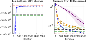
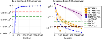
This section considers the task of estimating a static planted subspace from low-rank data corrupted by heterogeneous noise. We generate data according to the model in 1 with ambient dimension $d=100$ from a rank-3 subspace with squared singular values $[4,2,1]$, drawing 500 samples with noise variance $10^{-2}$, and 2,000 samples with noise variance $10^{-1}$. We draw an orthonormal subspace $\bm{U}\in\mathbb{R}^{100\times 3}$ uniformly at random from the Stiefel manifold, and set the planted factor matrix to be $\bm{F}=\bm{U}\sqrt{\bm{\lambda}}$.

After randomly permuting the order of the data vectors, we compared SHASTA-PCA to PETRELS and the streaming PCA algorithm GROUSE [19] (which has recently been shown to be equivalent to Oja’s method [22] in [47]) that estimates a subspace from rank-one gradient steps on the Grassmann manifold, with a tuned step size of $0.01$. SHASTA-PCA jointly learns both the factors $\bm{F}$ and noise variances $\bm{v}$ from each streaming observation. For SHASTA-PCA, we used $w_{t}=1/t$ (where $t$ is the time index), $c_{F}=c_{v}=0.1$ and initialize the parameters $\bm{\mkern 3.0mu\overline{\mkern-3.0muR\mkern-1.0mu}\mkern 1.0mu}_{t}(i)=\delta\bm{I}$ with $\delta=0.1$ for both SHASTA-PCA and PETRELS. We initialized each streaming algorithm with the same random $\bm{F}_{0}$, and each entry of $\bm{v}_{0}$ for SHASTA-PCA uniformly at random between 0 and 1. We set the forgetting parameter in PETRELS to $\lambda=1$, corresponding to the algorithm’s batch mode. As a baseline, we compared to batch algorithms for fully-observed data: HePPCAT [1] with 100 iterations, which we found to be sufficient for convergence, and homoscedastic probabilistic PCA (PPCA) [48] on the full data. In addition, we computed PPCA over each data group individually, denoted by “G1” (“G2”) in the legend of Fig. 1a corresponding to group 1 (2) with 500 (2,000) samples with noise variances $10^{-2}$ ($10^{-1}$) respectively.

The first experiment in Fig. 1a compares each algorithm in the fully observed data setting, where the streaming algorithms compute $\bm{F}$ and $\bm{v}$ incrementally using a single vector in each iteration. Given the planted model parameters $\bm{F}^{*}$ and $\bm{v}^{*}$ and their log-likelihood value $\mathcal{L}^{*}:=\mathcal{L}(\bm{F}^{*},\bm{v}^{*})$, the left plot in Fig. 1a shows the normalized log-likelihood $\mathcal{L}(\bm{F}_{t},\bm{v}_{t})-\mathcal{L}^{*}$ with respect to the full dataset in 2 for each iteration of SHASTA-PCA compared to the batch algorithm baselines. Because GROUSE and PETRELS do not estimate the noise variances, we omit them from this plot. The right plot in Fig. 1a shows convergence of the $\bm{F}$ iterates with respect to the normalized subspace error $\frac{1}{k}\|\hat{\bm{U}}_{t}\hat{\bm{U}}_{t}^{\prime}-\bm{U}\bm{U}^{\prime}\|_{F}^{2}$ for the estimate $\hat{\bm{U}}_{t}\in\mathbb{R}^{d\times k}$ of the planted subspace $\bm{U}$; for SHASTA-PCA and PETRELS, we compute $\hat{\bm{U}}_{t}$ by taking the $k$ left singular vectors of $\bm{F}$. Each figure plots the mean of 50 random initializations in bold dashed traces, where their standard deviations are displayed as ribbons. The experiment in Fig. 1b then subsamples 50% of the data entries uniformly at random, inserting zeros for the missing entries for methods that require fully sampled data, and compares the same statistics across the algorithms.

As expected, when the samples were fully observed, PETRELS converged to the same log-likelihood and subspace error for each set of training data as the batch algorithms that assume homoscedastic noise, and SHASTA-PCA converged to the same log-likelihood value and subspace error as HePPCAT. Here we see the advantage of using heteroscedastic data analysis. Instead of discarding the samples from either data group or combining them in a single PPCA, the heteroscedastc PPCA algorithms leverage both the “clean” samples, the additional “noisy” samples, and the noise variance estimates to produce better subspace estimates. With many missing entries (imputed with zero), the batch algorithms’ subspace estimates quickly deteriorated, as seen on the right-hand side of Fig. 1b. Out of the streaming PCA algorithms for missing data, SHASTA-PCA again attained the best subspace estimate compared to GROUSE and PETRELS.

(a) Fully observed data.

(b) Data with 50% entries observed uniformly at random.

Figure 1: Incremental computation (with one pass) over batch data generated from a static subspace for $d=100$, $n_{1}=500$, $n_{2}=2{,}000$, $v_{1}=10^{-2}$, and $v_{2}=10^{-1}$. Horizontal dashed lines correspond to the terminal values of batch algorithms, and the horizontal axis refers to streaming iteration for online algorithms.

7.2 Dynamic subspace

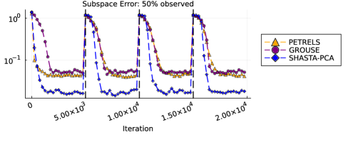
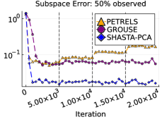
This section studies how well SHASTA-PCA can track a time-varying subspace. We generate 20,000 streaming data samples according to the model in 1 for some $\bm{F}=\bm{U}\sqrt{\bm{\lambda}}$, where $d=100$ and $\bm{\lambda}=[4,2,1]$, and noise variances $v_{1}=10^{-4}$ and $v_{2}=10^{-2}$, where the data are drawn from the two groups with 20% and 80% probability, respectively. We then observe 50% of the entries selected uniformly at random. To simulate dynamic jumps of the model, we set the planted subspace $\bm{U}$ to a new random draw every 5000 samples and compare the subspace errors of the various methods with respect to the current $\bm{U}$ over time. Here, we use the parameters $w_{t}=0.01,c_{F}=0.01$, and $c_{v}=0.1$ for SHASTA-PCA. After hyperparameter tuning, we set the step size of GROUSE to be 0.02, and we set $\lambda=0.998$ for PETRELS. Each algorithm is initialized with the same random factors $\bm{F}_{0}$, and SHASTA-PCA’s noise variances are initialized uniformly at random between 0 and 1. Fig. 2 shows SHASTA-PCA outperforms the streaming PCA algorithms that assume homoscedastic noise by half an order of magnitude. The results highlight how the largest noise variance dominates the streaming PCA algorithms’ subspace tracking while SHASTA-PCA obtains more faithful estimates of each $\bm{U}$.

Figure 2: Dynamic tracking of rapidly shifting subspace with 50% of the entries observed uniformly at random using SHASTA-PCA versus streaming PCA algorithms that assume homoscedastic noise. Here, $d=100$ and 20% of the data has noise variance $10^{-4}$ and $80\%$ of the data has noise variance $10^{-2}$. Iterations refers to the number of streamed data vectors.

7.3 Dynamic noise variances

In some applications, due to temperature, age, or change in calibration, the quality of the sensor measurements may also change with time [13], thereby affecting the levels of noise in the data. To study the performance of SHASTA-PCA in these settings, we generate samples from the planted model described above where we change the noise variances over time while keeping the subspace stationary. As before, SHASTA-PCA is initialized at a random $(\bm{F}_{0},\bm{v}_{0})$. Figs. 3a and 3c show the estimated noise variances and the subspace error as we double the noise variance of the first group every 5,000 samples. Figs. 3b and 3d repeat the experiment but double the noise variance of the second group instead. As $v_{1}$ increases and the cleaner group becomes noisier, the data becomes noisier overall and also closer to homoscedastic. SHASTA-PCA’s estimate of the subspace degrades and approaches the estimates obtained by PETRELS and GROUSE. On the other hand, as the noisier group gets even noisier, the quality of the PETRELS subspace estimate deteriorates in time whereas SHASTA-PCA remains robust to the added noise by leveraging the cleaner data group. In both instances, GROUSE appears to oscillate about an optimum in a region whose size depends on the two noise variances. The variance estimates demonstrate how SHASTA-PCA can quickly adapt to changes in the noise variances; SHASTA-PCA adapted here within less than 1,000 samples.

(a) Estimated variances for varying $v_{1}$.

(b) Estimated variances for varying $v_{2}$

(c) Subspace error with varying $v_{1}$.

(d) Subspace error with varying $v_{2}$.

Figure 3: Experiments with changing variances across time (iterations) for a single $\bm{F}\in\mathbb{R}^{100\times 3}$ starting with planted noise variances $\bm{v}=[10^{-4},10^{-2}]$ with 50% of the entries observed uniformly at random. The vertical dashed lines indicate points at which we double one of the planted variances. The top plots show the estimated variances from SHASTA-PCA, and the bottom plots show the subspace error.

7.4 Real data from astronomy

We illustrate SHASTA-PCA on real astronomy data from the Sloan Digital Sky Survey (SDSS) Data Release 16 [2] using the associated DR16Q quasar catalog [49]. In particular, we considered the subset that was considered in [10, Section 8]; see [10, Supplementary Material SM5] for details about the subset selected and the preprocessing performed. The dataset contains $n=$ 10,459 quasar spectra, where each spectrum is a vector of $d=281$ flux measurements across wavelengths and the data come with associated noise variances.

Ordering the samples from smallest to largest noise variance estimates, we obtained a “ground-truth” signal subspace by taking the left $k=5$ singular vectors of the data matrix for the first 2,000 samples with the smallest noise variance estimates. We then formed a training dataset with two groups: first, we collected samples starting from sample index 6,500 to the last index where the noise variance estimate is less than or equal to 1 (7,347); second, we collected training data beginning at the first index where the noise variance estimate is greater than or equal to 2 (8,839) up to the sample index 10,449, excluding the last 10 samples that are grossly corrupted by noise. The resulting training dataset had $n_{1}=848$ and $n_{2}=$ 1,611 samples for the two groups, respectively, and had strong noise heteroscedasticity across the samples, where the second group was much noisier than the first. Fig. 4a shows the training dataset and the associated noise variance estimates for each sample.

(a)

(b)

Figure 4: (a) Visualization of quasar data with true associated variances of each sample plotted by quasar. The estimated variances from a SHASTA-PCA $L=n$ model streaming over the samples (fully sampled, in randomized order) closely matched the true variances. (b) For fully sampled data, the subspace error of SHASTA-PCA converged to the error of HePPCAT’s estimated subspace for a $L=n$ model. We repeated the experiment 50 times, each with a different random initialization and order of the samples.

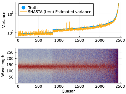
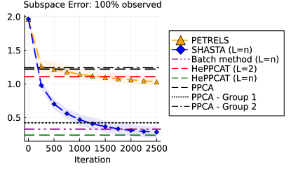
Although we formed the data by combining two groups of consecutive samples, the data actually contained $L=n$ groups since each spectrum has its own noise variance. This setting allows for a heuristic computational simplification in SHASTA-PCA. Namely, we adapt the $L=1$ model for a single variance $v$ and use separate weights for the SMM updates of $\bm{F}$ and $v$, where $w_{t}^{(F)}=0.001$, $c_{F}=0.1$, and $w_{t}^{(v)}=c_{v}=1$ $\forall t$. The variance update is then equivalent to maximizing $\Psi_{t}(\bm{F}_{t-1},v;\bm{F}_{t-1},v_{t-1})$, i.e., the minorizer centered at the previous variance estimate with no memory of previous minorizers. The number of variance EM updates per data vector may be increased beyond just a single update, but in practice, we observed little additional benefit. Fig. 4 shows how SHASTA-PCA adaptively learned the unknown variances for each new sample and converged to the same level of subspace error as the batch HePPCAT $L=n$ model.

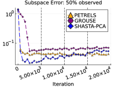
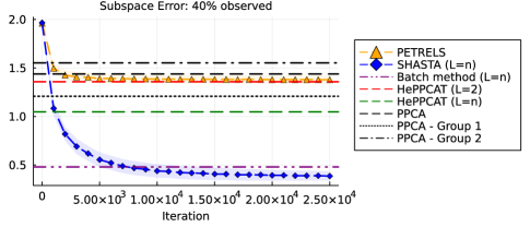
In many modern large datasets, entries may be missing in significant quantities due to sensor failure or time and memory constraints that preclude acquiring complete measurements. Indeed, the experiment designer may only wish to measure a “sketch” of the full data to save time and resources and learn the underlying signal subspace from limited observations using an algorithm like SHASTA-PCA. To study this case, we randomly obscured 60% of the entries uniformly at random and performed 10 passes over the data, randomizing the order of the samples each time. Again, we use the same choice of weights described above to estimate a single variance for every new sample. We initialized with a random $\bm{F}_{0}$ and $v_{0}$ using the zero-padded data. As Fig. 5 shows, SHASTA-PCA had better subspace estimates in this limited sampling setting than the state-of-the-art baseline methods with zero-filled missing entries and/or homoscedastic noise assumptions. Interestingly, the SHASTA-PCA subspace estimate was even better than the batch method in Section 5 for the $L=n$ model.

Figure 5: Subspace error for quasar data with 40% of the entries observed uniformly at random. SHASTA-PCA streams over the full dataset 10 times, with the sample entries missing, where the order of the samples was randomized on each pass. Each experiment was initialized with factors chosen uniformly at random.

7.5 Computational timing experiments

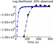
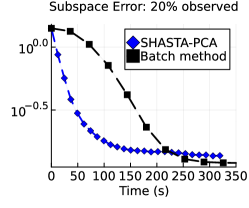
Computational and/or storage considerations can inhibit the use of batch algorithms for large datasets, especially on resource constrained devices. To demonstrate the benefit of SHASTA-PCA in such settings, we generated a 2GB dataset according to our model, where $d=1{,}000$, $\bm{\lambda}=[4,2,1]$, $\bm{n}=[50{,}000,~{}200{,}000]$, $\bm{v}=[0.1,1]$, and we observed only 20% of the entries uniformly at random. For this experiment, we set $w_{t}=0.01/\sqrt{t}$, $c_{F}=0.01$, and $c_{v}=0.1$ for SHASTA’s hyperparameters, and passed over the entire data once. Fig. 6 compares the convergence in log-likelihood values and subspace errors by elapsed wallclock time for SHASTA and the batch algorithm in Section 5, where both algorithms are randomly initialized from the same random starting iterate $(\bm{F}_{0},\bm{v}_{0})$. SHASTA-PCA rapidly obtained a good estimate of the model, using only roughly 60% of the time that it took the batch method, all while using only 0.0048% of the memory per iteration.

(a)

(b)

Figure 6: Log-likelihood values and subspace errors versus elapsed wall clock time for one run of SHASTA-PCA versus the batch method in Section 5 on 2GB of synthetic data: $d=1{,}000$, $k=3$, $\bm{n}=[50{,}000,~{}200{,}000]$, and $\bm{v}=[0.1,1]$. Both algorithms used the same random initialization. Markers for SHASTA-PCA are for every $10{,}000$ vector samples, and markers for the batch method are for each algorithm iteration.

8 Conclusion & Future Work

This paper proposes a new streaming PCA algorithm that is robust to both missing data and heteroscedastic noise across samples. The stochastic MM approach only requires a modest amount of memory independent of the number of samples and has efficient updates that can scale to large datasets. The results show significant improvement over state-of-the-art streaming PCA algorithms in tracking nonstationary subspaces under heteroscedastic noise and significant improvement over a batch algorithm in rapid model estimation.

There are many future directions building on this work. First, proving convergence of SHASTA-PCA is of key interest. Second, while each update of a row in $\bm{F}$ is relatively cheap, it still requires inverting $|\Omega_{t}|$ many $k\times k$ matrices per data vector, which is particularly wasteful when $|\Omega_{t}|=d$ since this is equivalent to the fully sampled log-likelihood that only requires a single $k\times k$ inverse to update $\bm{F}$. It may be possible to find looser surrogate functions that would avoid this large number of small inverses in each iteration. While our streaming algorithms enjoy lightweight computations in each iteration, achieving rapid convergence can depend on the careful tuning of the weights $w_{t}$ and the parameters $c_{F}$ and $c_{v}$. Adaptively selecting these parameters with stochastic MM techniques and developing theory to guide the selection of these parameters remain open problems.

Perhaps the most immediate and important line of future work is to establish convergence guarantees for SHASTA-PCA. Our setting differs in several key ways from the prior works discussed in Section 2 that establish convergence for SMM algorithms. First, our minorizers are neither Lipschitz smooth nor strongly concave (in fact, the minorizer for $v_{\ell}$ is nonconcave), so the theory in [5] does not directly apply. Second, our algorithm maximizes the log-likelihood in two blocks of variables, and does so in an alternating way using two separate approximate minorizers $\bar{\Psi}_{t}^{(F)}(\bm{F})$ and $\bar{\Psi}_{t}^{(v)}(\bm{v})$, which is distinct from the work in [26] that alternates updates over the blocks of a single joint approximate minorizer. Notably, such as in the case of $\bm{v}$, we update an aggregation $\bar{\Psi}_{t}^{(v)}(\bm{v})$ of the restricted minorizers $\Psi_{i}(\bm{F}_{i-1},\bm{v};\bm{F}_{i-1},\bm{v}_{i-1})$:

$$\bar{\Psi}_{t}^{(v)}(\bm{v})=(1-w_{t})\bar{\Psi}_{t-1}^{(v)}(\bm{v})+w_{t}\Psi_{t}(\bm{F}_{t-1},\bm{v};\bm{F}_{t-1},\bm{v}_{t-1})$$

$$=\sum_{i=0}^{t}\left[{w_{i}\prod_{j=i+1}^{t}(1-w_{j})}\right]\,\Psi_{i}(\bm{F}_{i-1},\bm{v};\bm{F}_{i-1},\bm{v}_{i-1}).$$ (42)

The dependence of $\bar{\Psi}_{t}^{(v)}(\bm{v})$ on all past iterates $\{\bm{F}_{i}\}_{i=0}^{t}$ in the first argument of each $\Psi_{i}$ in 42 precludes using the analysis of [26] for BCD of a single approximate minorizer each iteration. However, we conjecture similar convergence guarantees are possible for SHASTA-PCA since both $\bar{\Psi}_{t}^{(F)}(\bm{v})$ and $\bar{\Psi}_{t}^{(v)}(\bm{v})$ retain many of the same MM properties used in the techniques to analyze SMM algorithms.

References

- [1] D. Hong, K. Gilman, L. Balzano, and J. A. Fessler, “HePPCAT: Probabilistic PCA for data with heteroscedastic noise,” IEEE Transactions on Signal Processing, vol. 69, pp. 4819–4834, 2021.
- [2] R. Ahumada, C. A. Prieto, A. Almeida, F. Anders, S. F. Anderson, B. H. Andrews, B. Anguiano, R. Arcodia, E. Armengaud, M. Aubert et al., “The 16th data release of the sloan digital sky surveys: first release from the APOGEE-2 southern survey and full release of eBOSS spectra,” The Astrophysical Journal Supplement Series, vol. 249, no. 1, p. 3, 2020.
- [3] K. P. Pruessmann, M. Weiger, M. B. Scheidegger, and P. Boesiger, “SENSE: sensitivity encoding for fast MRI,” Magnetic Resonance in Medicine: An Official Journal of the International Society for Magnetic Resonance in Medicine, vol. 42, no. 5, pp. 952–962, 1999.
- [4] C. Anam, K. Adi, H. Sutanto, Z. Arifin, W. Budi, T. Fujibuchi, and G. Dougherty, “Noise reduction in CT images with a selective mean filter,” J Biomed Phys Eng., vol. 10, pp. 623–634, 09 2020.
- [5] A. Mensch, J. Mairal, B. Thirion, and G. Varoquaux, “Stochastic subsampling for factorizing huge matrices,” IEEE Transactions on Signal Processing, vol. 66, no. 1, pp. 113–128, 2017.
- [6] E. J. Candes and Y. Plan, “Matrix completion with noise,” Proceedings of the IEEE, vol. 98, no. 6, pp. 925–936, 2010.
- [7] K. Ni, N. Ramanathan, M. N. H. Chehade, L. Balzano, S. Nair, S. Zahedi, E. Kohler, G. Pottie, M. Hansen, and M. Srivastava, “Sensor network data fault types,” ACM Trans. Sen. Netw., vol. 5, no. 3, jun 2009. [Online]. Available: https://doi.org/10.1145/1525856.1525863
- [8] I. T. Jolliffe, Principal Component Analysis. Springer-Verlag, 2002.
- [9] G. Young, “Maximum likelihood estimation and factor analysis,” Psychometrika, vol. 6, no. 1, pp. 49–53, Feb. 1941.
- [10] D. Hong, F. Yang, J. A. Fessler, and L. Balzano, “Optimally weighted PCA for high-dimensional heteroscedastic data,” SIAM Journal on Mathematics of Data Science, vol. 5, no. 1, pp. 222–250, Mar. 2023.
- [11] A. R. Zhang, T. T. Cai, and Y. Wu, “Heteroskedastic PCA: Algorithm, optimality, and applications,” The Annals of Statistics, vol. 50, no. 1, pp. 53–80, 2022.
- [12] Y. Chi, Y. C. Eldar, and R. Calderbank, “PETRELS: Parallel subspace estimation and tracking by recursive least squares from partial observations,” IEEE Transactions on Signal Processing, vol. 61, no. 23, pp. 5947–5959, 2013.
- [13] L. Jun-hua, S. Zhong-ru et al., “Drift reduction of gas sensor by wavelet and principal component analysis,” Sensors and Actuators B: Chemical, vol. 96, no. 1-2, pp. 354–363, 2003.
- [14] L. Balzano, Y. Chi, and Y. M. Lu, “Streaming PCA and subspace tracking: The missing data case,” Proceedings of the IEEE, vol. 106, no. 8, pp. 1293–1310, 2018.
- [15] D. P. Bertsekas, “Incremental gradient, subgradient, and proximal methods for convex optimization: A survey,” Optimization for Machine Learning, vol. 2010, no. 1-38, p. 3, 2011.
- [16] L. Bottou, “Large-scale machine learning with stochastic gradient descent,” in Proceedings of COMPSTAT’2010, Y. Lechevallier and G. Saporta, Eds. Heidelberg: Physica-Verlag HD, 2010, pp. 177–186.
- [17] M. Mardani, G. Mateos, and G. B. Giannakis, “Subspace learning and imputation for streaming big data matrices and tensors,” IEEE Transactions on Signal Processing, vol. 63, no. 10, pp. 2663–2677, 2015.
- [18] S. Bonnabel, “Stochastic gradient descent on riemannian manifolds,” IEEE Transactions on Automatic Control, vol. 58, no. 9, pp. 2217–2229, 2013.
- [19] L. Balzano, R. D. Nowak, and B. Recht, “Online identification and tracking of subspaces from highly incomplete information,” 2010 48th Annual Allerton Conference on Communication, Control, and Computing (Allerton), pp. 704–711, 2010.
- [20] J. He, L. Balzano, and J. C. S. Lui, “Online robust subspace tracking from partial information,” CoRR, vol. abs/1109.3827, 2011. [Online]. Available: http://arxiv.org/abs/1109.3827
- [21] J. Goes, T. Zhang, R. Arora, and G. Lerman, “Robust stochastic principal component analysis,” in Artificial Intelligence and Statistics. PMLR, 2014, pp. 266–274.
- [22] E. Oja, “Simplified neuron model as a principal component analyzer,” Journal of Mathematical Biology, vol. 15, pp. 267–273, 1982.
- [23] A. Henriksen and R. Ward, “AdaOja: Adaptive learning rates for streaming PCA,” arXiv preprint arXiv:1905.12115, 2019.
- [24] J. A. Fessler, “Lecture notes for optimization methods for signal and image processing (EECS 598), chapter 4,” 2019.
- [25] J. Mairal, “Stochastic majorization-minimization algorithms for large-scale optimization,” in Advances in Neural Information Processing Systems, C. J. C. Burges, L. Bottou, M. Welling, Z. Ghahramani, and K. Q. Weinberger, Eds., vol. 26. Curran Associates, Inc., 2013. [Online]. Available: https://proceedings.neurips.cc/paper/2013/file/4da04049a062f5adfe81b67dd755cecc-Paper.pdf
- [26] C. Strohmeier, H. Lyu, and D. Needell, “Online nonnegative tensor factorization and CP-dictionary learning for markovian data,” ArXiv, vol. abs/2009.07612, 2020.
- [27] H. Lyu, “Convergence and complexity of stochastic block majorization-minimization,” arXiv preprint arXiv:2201.01652, 2022.
- [28] A. Mokhtari and A. Koppel, “High-dimensional nonconvex stochastic optimization by doubly stochastic successive convex approximation,” IEEE Transactions on Signal Processing, vol. 68, pp. 6287–6302, 2020.
- [29] M. E. Tipping and C. M. Bishop, “Probabilistic Principal Component Analysis,” Journal of the Royal Statistical Society: Series B (Statistical Methodology), vol. 61, no. 3, pp. 611–622, Aug. 1999.
- [30] J. A. S. Cavazos, J. A. Fessler, and L. Balzano, “Alpcah: Sample-wise heteroscedastic pca with tail singular value regularization,” in Fourteenth International Conference on Sampling Theory and Applications, 2023.
- [31] A. S. Xu, L. Balzano, and J. A. Fessler, “Hemppcat: Mixtures of probabilistic principal component analysers for data with heteroscedastic noise,” in ICASSP 2023 - 2023 IEEE International Conference on Acoustics, Speech and Signal Processing (ICASSP), 2023, pp. 1–5.
- [32] M. E. Tipping and C. M. Bishop, “Mixtures of probabilistic principal component analyzers,” Neural computation, vol. 11, no. 2, pp. 443–482, 1999.
- [33] W. Leeb and E. Romanov, “Optimal spectral shrinkage and PCA with heteroscedastic noise,” IEEE Transactions on Information Theory, vol. 67, no. 5, pp. 3009–3037, 2021.
- [34] W. E. Leeb, “Matrix denoising for weighted loss functions and heterogeneous signals,” SIAM Journal on Mathematics of Data Science, vol. 3, no. 3, pp. 987–1012, 2021.
- [35] D. Hong, Y. Sheng, and E. Dobriban, “Selecting the number of components in pca via random signflips,” 2020. [Online]. Available: http://arxiv.org/abs/2012.02985v1
- [36] Z. T. Ke, Y. Ma, and X. Lin, “Estimation of the number of spiked eigenvalues in a covariance matrix by bulk eigenvalue matching analysis,” Journal of the American Statistical Association, vol. 118, no. 541, pp. 374–392, jul 2021.
- [37] B. Landa, T. T. C. K. Zhang, and Y. Kluger, “Biwhitening reveals the rank of a count matrix,” SIAM Journal on Mathematics of Data Science, vol. 4, no. 4, pp. 1420–1446, dec 2022.
- [38] J. K. Behne and G. Reeves, “Fundamental limits for rank-one matrix estimation with groupwise heteroskedasticity,” in International Conference on Artificial Intelligence and Statistics. PMLR, 2022, pp. 8650–8672.
- [39] A. Breloy, G. Ginolhac, A. Renaux, and F. Bouchard, “Intrinsic Cramér–Rao bounds for scatter and shape matrices estimation in CES distributions,” IEEE Signal Processing Letters, vol. 26, no. 2, pp. 262–266, Feb. 2019.
- [40] A. H. Ferrer, M. N. El Korso, A. Breloy, and G. Ginolhac, “Robust mean and covariance matrix estimation under heterogeneous mixed-effects model with missing values,” Signal Processing, vol. 188, p. 108195, 2021.
- [41] A. Hippert-Ferrer, M. El Korso, A. Breloy, and G. Ginolhac, “Robust low-rank covariance matrix estimation with a general pattern of missing values,” Signal Processing, vol. 195, p. 108460, 2022. [Online]. Available: https://www.sciencedirect.com/science/article/pii/S016516842200007X
- [42] A. Collas, F. Bouchard, A. Breloy, G. Ginolhac, C. Ren, and J.-P. Ovarlez, “Probabilistic PCA from heteroscedastic signals: Geometric framework and application to clustering,” IEEE Transactions on Signal Processing, vol. 69, pp. 6546–6560, 2021.
- [43] S. Song, K. Chaudhuri, and A. D. Sarwate, “Learning from data with heterogeneous noise using SGD,” Journal of Machine Learning Research, vol. 38, pp. 894–902, 2015.
- [44] D. Hong, L. Balzano, and J. A. Fessler, “Probabilistic PCA for heteroscedastic data,” in 8th IEEE International Workshop on Computational Advances in Multi-Sensor Adaptive Processing, 2019, pp. 26–30.
- [45] D. P. O’Leary, “Near-optimal parameters for tikhonov and other regularization methods,” SIAM Journal on scientific computing, vol. 23, no. 4, pp. 1161–1171, 2001.
- [46] K. Cao, Y. Chen, J. Lu, N. Arechiga, A. Gaidon, and T. Ma, “Heteroskedastic and imbalanced deep learning with adaptive regularization,” arXiv preprint arXiv:2006.15766, 2020.
- [47] L. Balzano, “On the equivalence of Oja’s algorithm and GROUSE,” in International Conference on Artificial Intelligence and Statistics. PMLR, 2022, pp. 7014–7030.
- [48] M. Tipping and C. Bishop, “Probabilistic principal component analysis,” J. Royal Stat. Soc. Ser. B, vol. 6, pp. 611–22, 1999.
- [49] B. W. Lyke, A. N. Higley, J. McLane, D. P. Schurhammer, A. D. Myers, A. J. Ross, K. Dawson, S. Chabanier, P. Martini, H. D. M. Des Bourboux et al., “The Sloan Digital Sky Survey Quasar Catalog: Sixteenth data release,” The Astrophysical Journal Supplement Series, vol. 250, no. 1, p. 8, 2020.