Quantum state tomography with disentanglement algorithm

Abstract

In this work, we report on a novel quantum state reconstruction process based on the disentanglement algorithm. Using variational quantum circuits, we disentangle the quantum state to a product of computational zero states. Inverse evolution of the zero states reconstructs the quantum state up to an overall phase. By sequentially disentangling the qubit one by one, we reduce the required measurements with only single qubit measurement. Demonstrations with our proposal for the reconstruction of the random states are presented where variational quantum circuit is optimized by disentangling process. To facilitate experimental implementation, we also employ reinforcement learning for quantum circuit design with limited discrete quantum gates. Our method is universal and imposes no specific ansatz or constraint on the quantum state.

Introduction.– The quantum state reconstruction through measurements on identical quantum states, known as quantum state tomography, is important for benchmarking and verification of quantum system and quantum device. Although fully determination of the quantum state has already been achieved by using a complete set of observables QuantumStateEstimation ; Hou_2016 , the exponential scaling required in system size is inefficient. Broad efficient learning techniques have been developed to avoid the exponential scaling such as machine learning methods using neural networks science.aag2302 ; PhysRevA.102.022412 ; PhysRevLett.123.230504 ; PhysRevA.104.012401 ; Palmieri2020 ; Carrasquilla2019 ; Torlai2018 , Bayesian inference incorporating with prior knowledge RevModPhys.81.299 ; PhysRevA.61.010304 ; PhysRevLett.108.070502 ; PhysRevA.95.062336 ; Granade_2016 ; Granade_2017 ; Blume-Kohout_2010 , and tensor network representations DBLP ; YiKai2010 ; Lanyon2017 ; PhysRevLett.111.020401 ; PhysRevA.101.032321 . One important feature distinguishing the quantum many body system and the classical system is the existence of entanglement arising from the connections between different parts of the system RevModPhys.81.865 . Correlations of the subsystems require exponentially many parameters in system size to fully characterize the system state. A quantum state without entanglement will be much easier to characterize. Here, we propose a novel protocol for quantum state tomography with disentanglement algorithm.

By transforming of the unknown quantum state into zero-product state, the quantum state can be efficiently reconstructed by inverse transformation from the product state up to an overall phase factor. In the disentanglement process, we need to identify the unitary transformation or the quantum circuit configuration. In this work, we present two methods to generate the unitary transformation. One relies on the variational quantum circuit, while the other relies on the reinforcement learning method for limited discrete quantum gates. To deal with the measurement complexity during the training process, sequential disentangling the qubit one by one is introduced where only single qubit measurement is required. In the following, we numerically demonstrated that sequential disentanglement scheme can efficiently reconstruct the quantum state.

Disentanglement protocol.– In general, it is possible to evolve an unknown pure quantum state into a product state by an unitary transformation. For the quantum state with $N$ qubits, the disentanglement process needs to remove all the entanglement between any two subsystems. We propose disentanglement scheme where the entanglement is removed sequentially.

Figure 1: Sequential disentanglement scheme with variational quantum circuits. Here taking total number of qubits as $N=5$ for demonstration. $|\psi\rangle$ is the unknown quantum state to be measured or reconstructed. The overall disentangled transformation $\hat{\mathcal{U}}$ is composed by five disentangled circuits $\hat{U}_{j}$.

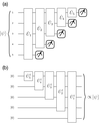
As shown in Fig. 1 (a), taking $N=5$ for example, we construct the disentangled transformation $\hat{\mathcal{U}}$ with a series of variational quantum circuits $\hat{U}_{j}$ such that

$$|0\rangle^{\otimes N}\propto~{}\hat{\mathcal{U}}|\psi\rangle=\Pi_{j=N}^{j=1}\hat{U}_{j}|\psi\rangle,$$ (1)

where $\propto$ stands for a difference up to an overall phase factor.

Figure 2: Quantum circuit configuration for the parametric quantum circuit $\hat{U}_{1}$ with qubit number $N=5$. The building block is composed by product of $N=5$ parametrized single qubit unitary rotations and $N-1$ CNOT gates. Five copies of the building blocks compose the quantum circuit $\hat{U}_{1}$.

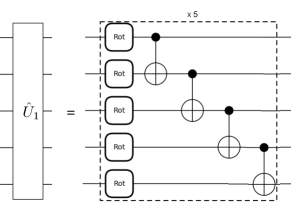
Within the disentanglement transformation $\hat{\mathcal{U}}$, each parametric quantum circuit $\hat{U}_{j}$ is responsible for disentangling the last qubit of the applied system in Fig. 1 (a) where the measurement is applied on. To remove the disentanglement, the parametric circuit is designed with configuration given by Fig. 2. The building block is composed of $N$ single qubit gates and $N-1$ CNOT gates. Multiple copies of the building blocks enhance the disentangled ability. The training parameters are included in the single rotational gate with

$$\hat{V}_{\rm rot}(\phi,\theta,\omega)=\begin{bmatrix}\cos\frac{\theta}{2}e^{-i\frac{\phi+\omega}{2}}&-\sin\frac{\theta}{2}e^{i\frac{\phi-\omega}{2}}\\ \sin\frac{\theta}{2}e^{-i\frac{\phi-\omega}{2}}&\cos\frac{\theta}{2}e^{i\frac{\phi+\omega}{2}}\end{bmatrix}.$$ (2)

Instead of determining the whole transformation $\hat{\mathcal{U}}$ together, as shown in Fig. 1, in the first sequence, we will determine $\hat{U}_{1}$ through measurement probability on fifth qubit by requiring the disentanglement between this qubit and the other part of the system. In this sequence, only parameters within $\hat{U}_{1}$ are updated by requiring the probability of the last qubit at zero state to be maximum with $m_{5}={\rm Tr}\{{\rm I}^{\otimes 4}\otimes|0\rangle\langle 0|\cdot|\phi_{q}\rangle\langle\phi_{q}|\}$. Here $|\phi_{q}\rangle$ is the evolved state with the number of qubits $q$, which is related to the initial state through $|\phi_{q=5}\rangle=\hat{U}_{1}|\psi\rangle$. During training, we choose the loss function as

$$\mathcal{L}=1-{\rm m}_{q},$$ (3)

where the general single qubit measurement in each sequence can be written as

$${\rm m}_{q}={\rm Tr}\{\hat{P}_{0}^{q}|\phi_{q}\rangle\langle\phi_{q}|\},$$ (4)

with the corresponding projection operator $\hat{P}_{0}^{q}={\rm I}^{\otimes(q-1)}\otimes|0\rangle\langle 0|$. After training by gradient descent, the loss reaches zero and the fifth qubit obtains a state of $|0\rangle$. Then the evolved state can be casted in the form of

$$|\phi_{q}\rangle=|\psi_{q-1}\rangle\otimes|0\rangle,$$ (5)

where $|\psi_{q-1}\rangle$ can be viewed as the reduced initial state for the disentangled subsystem.

Figure 3: Training loss for all iterations with total number of qubits $N=5$. In the first iteration, for qubit $=5$, the red line with circles denote the loss $\mathcal{L}$ trajectory during training process and the red line $\mathcal{P}$ denotes the purity of the subsystem. Similar results are presented for iteration $2,3,4$ with qubit $=4,3,2$ respectively. For the last iteration with qubit $=1$, purity is always one and loss approaches zero in terms of training epochs.

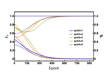
Taking a random quantum state with $N=5$ qubits for example, the training results are displayed in Fig. 3. In the first training sequence, the loss function $\mathcal{L}$ is trained as shown by the red line with open circles in Fig. 3. When $\mathcal{L}$ approaches zero, the measurement result for the fifth qubit will always be zero and disentanglement is acquired. In the second training sequence, similar training procedures are applied to $\hat{U}_{2}$ with $\hat{U}_{1}$ fixed. By repeating the disentanglement procedures, we identify the quantum circuits $\hat{U}_{j}$ one by one through the result of measurement probability of the associated single qubit. It can be found that the loss function for all the sequences reach zero within numerical precision after training. To monitor the disentangled process, purity of the subsystem is calculated as

$$\mathcal{P}={\rm Tr}\{\hat{\rho}_{\rm sub}^{2}\}.$$ (6)

Here $\hat{\rho}_{\rm sub}={\rm Tr}_{\rm q}|\phi_{q}\rangle\langle\phi_{q}|$ where the last qubit is partially traced out. When there is no coupling between the last qubit and the subsystem, $\mathcal{P}$ approaches one, which indicates that both of them are pure states. In each training sequence, the corresponding purity $\mathcal{P}$ of the reduced subsystem is plotted with solid line in Fig. 3. At the end of training, all the loss functions $\mathcal{L}$ and purities converge. The training results indicate the removal of all the correlations of the system. Noticing that the final state of each qubit may include a phase factor which cannot be resolved by measurement. Product of all the phase factors will contribute to an overall phase of the state. The overall evolved state can be written as product state of single qubit $|0\rangle$ with an overall phase factor.

Reconstruction process.–

Figure 4: Reconstruction fidelity $\mathcal{F}$ for quantum state in terms of qubit number $N$ with different training precisions $\overline{m}$.

Although the overall phase factor cannot be resolved by measurement, the quantum state can still be reconstructed by product of zero states $|0\rangle^{\otimes N}$. As shown in Fig. 1 (b), back propagation with the trained unitary transformations leads to the reconstructed state $|\psi^{\prime}\rangle$ as

$$|\psi^{\prime}\rangle=\Pi_{j=1}^{j=N}\hat{U}_{i}^{\dagger}|0\rangle^{\otimes N}.$$ (7)

The reconstructed state $|\psi^{\prime}\rangle$ differs from the quantum state $|\psi\rangle$ up to an overall phase factor, which is irrelevant for physical observable measurements. We define the fidelity $\mathcal{F}$ between the reconstructed state and the unknown quantum state as

$$\mathcal{F}=|\langle\psi|\psi^{\prime}\rangle|^{2}.$$ (8)

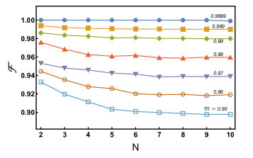
As shown in Fig. 4, the top line with $\mathcal{F}\approx 1$ where the loss are trained to be zero and the measurement results ${\rm m}_{q}$ are optimized to one for all the sequences with $\overline{m}=1/N\sum_{q}{\rm m}_{q}=1$ within machine precisions, the fidelity between the the reconstruction state and unknown state can be as high as one. Namely, we can reconstruct the unknown quantum state exactly in principle.

However, in reality, due to noise or decoherence effect, it will be difficult to obtain a $100\%$ probability. During each training sequences, when the loss $\mathcal{L}$ deviates from the optimized value by a small value, how will it affect on the reconstruction fidelity? As presented in Fig. 4, the fidelity deviates from one with smaller $\overline{m}$. The deviation is stronger for larger qubit numbers N. To reach a specific fidelity, higher precision is required for larger $N$. Results presented in Fig. 4 provides a guideline for the practical implementation.

From continuous to discrete.– For experimental implementation or most of the quantum platforms, the available gate operations are limited. Optimization procedure of variational quantum circuit proposed previously cannot be applied to this discrete problem. For limited discrete gate operations, we will utilize the reinforcement learning method 712192 for the quantum circuit design. We assume the following available single-qubit quantum gates:

$$\mathcal{G}=\{{\rm I,X,Y,Z,H,T,S}\},$$ (9)

and the two-qubit gate CNOT gate. Here ${\rm I}$ stands for identity, ${\rm X,Y,Z}$ are three Pauli gates, H is the Hadamard gate and S is the phase gate with ${\rm T}^{2}=S$. The quantum circuit will be constructed by the above quantum gates. Reinforcement learning as a machine learning paradigm can train a policy to make a sequence of decisions in an environment in order to maximize a reward signal NIPS1999_464d828b . Given a random quantum state (the environment), the trained policy is likely to generate the disentangled quantum gates configuration (sequence of decisions) with high probability.

For this discrete case, the ingredients for the quantum circuit design are the assumed single-qubit gates $g\in\mathcal{G}$ given by Eq. (9) and the two-qubit CNOT gate. Within the framework of reinforcement learning, the possible actions are chosen as the combined two-qubit gates represented by Fig. 5 (a).

Figure 5: (a) Possible combined two-qubit gates for the action in the reinforcement learning framework. The assumed two-qubit gate operation stands for the combination of the a single-qubit gate $g\in\mathcal{G}$ and a CNOT gate with operation explicitly given by ${\rm CNOT}\cdot g\otimes{\rm I}$. (b) Schematic of the quantum circuit configuration generated by the reinforcement learning method for disentangling the fifty qubit. In each layer, the two-qubit action is chosen from the action set $\mathcal{A}$.

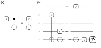
There are seven kinds of combined two-qubit gates available in the action set. For each two-qubit gate, we restrict that the first qubit operation can be applied to any qubit except the measurement qubit, and the second qubit can only be applied to the disentangling qubit to be measured. Thus for disentangling an $N$ qubit system, there are $N$ ways of qubit operation. Taking into account of seven types of gates, the total number of possible actions is $7N$, which will compose the disentangled quantum circuit according to the reinforcement learning algorithm as illustrated by Fig. 5(b). The action set can be denoted as $\mathcal{A}=\{a_{s}|s=1,2,...,7N\}$. Noting that for the sequential disentangling algorithm as shown in Fig. 1, the number of actions will decline in terms of sequence due to smaller disentangled system size.

In the reinforcement learning algorithm, we utilize the classical neural network to be the policy function which maps the states to the actions. The input state of the policy function will be denoted as an action sequence with fixed length $L$. Thus for the initial state, the input for the classical neural network is encoded as identity actions $\{{\rm I},{\rm I},...,{\rm I}\}$. For each input state, the classical neural network generates the probability of all the possible action $P(a_{s})$. The next action is sampled according to the probability distribution provided by the policy function (neural network). It is reasonable to set the measured probability after application of $a_{s}$ as the the reward function which justify the soundness of the action $a_{s}$. To maximize the reward or improve the measurement probability, the loss of the policy function is given by

$$loss=-\sum_{s}\log[P(a_{s})]\mathcal{R}(a_{s}),$$ (10)

where $\mathcal{R}(a_{s})$ is the reward function of action $a_{s}$ set as the measured probability of disentangled qubit evolved by action $a_{s}$. Training policy with the above loss function results in higher probability of the action $a_{s}$ with larger reward $\mathcal{R}(a_{s})$. Then a large reward will increase the probability of the corresponding action after training. The reinforcement learning procedures are as follows: (i) Training dataset generating: generating $\mathcal{D}$ action sequences with length $L$ according to the policy, and calculating the corresponding rewards for each action; (ii) Improving the policy performance: training the policy (classical neural network) using the dataset generated in (i) with loss given by Eq. (10). Repeating procedure (i) and (ii) until the reward of the action reaches the maximal value $100\%$, where the corresponding qubit is disentangled from the system. In this circumstance, we can disentangle a quantum state sequentially with the above reinforcement learning procedures.

Figure 6: Maximal reward (blue line) and average reward (yellow line) achieved durning reinforcement learning procedure. For each $100$ training epochs, one qubit will be disentangled from the system. For $N=5$ qubit system, each red star point provides the action sequence for the disentanglement quantum circuit design.

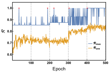
Setting the the length of action sequence $L=10$, dataset dimension $\mathcal{D}=50$ and the training epoch as $100$, the rewards of the actions in the dataset generated in step (i) during training are displayed in Fig. 6. For a random generated $N=5$ qubit quantum state, reinforcement learning procedures are applied to each qubit sequentially. Each qubit will be disentangled within $100$ training epochs. As shown in Fig. 6, focusing on the first $100$ training epochs (the first disentanglement sequence), the average and maximal rewards of $\mathcal{D}$ action sequences generated by the trained policy are plotted by the yellow and blue lines respectively. After training, the average rewards increase and maximal $\mathcal{R}_{\rm max}(a_{s})=1$ is obtained. Similar results are presented for other disentanglement sequences in Fig. 6. Noticing that it is possible that multiple $\mathcal{R}_{\rm max}$ appear during training. There exist multiple configurations for constructing the disentanglement transformation. In practice we can stop the training process when the first solution is obtained, which is denoted by the red star points in Fig. 6. The input and output of the policy function combined together compose the configuration of action sequence for the disentanglement transformation. Then the disentanglement quantum circuit configuration is successfully identified with help of the reinforcement learning method. Five disentanglement action sequences denoted by the red stars can be used to reconstruct the input unknown quantum state. It is worth noting that identifying a disentanglement quantum neural network configuration is not always guaranteed, such as when the action sequence is too short or the gate types is too limited to implement a disentanglement unitary transformation.

Summary and Outlook.– We propose a novel quantum state reconstruction process based on the disentanglement algorithm. Provided by the single qubit measurement result, we can identify the disentanglement transformation. We identify the transformation with variational quantum circuit optimization and reinforcement learning assistant circuit design. Both of them can successfully disentangle and reconstruct the target quantum state and implement the quantum state tomography task. The introduced sequential disentanglement scheme only require the single qubit measurement, which greatly reduce the measurement complexityPhysRevApplied.13.024013 . Our method is universal and imposes no specific ansatz or constrain on the quantum state, which can be applied to various circumstances. Besides quantum state tomography, our protocol can be generalized to problems such as Hamiltonian learning, gate decomposition, where quantum circuit design plays a role in the problems.

Acknowledgement. We thank Yadong Wu, Pengfei Zhang, Xiuhao Deng, and Georg Engelhardt for helpful discussions. This work is supported by Guangdong Basic and Applied Basic Research Foundation (2022B1515120021), National Natural Science Foundation of China (Grant No. 11904190) and the Science, Technology and Innovation Commission of Shenzhen, Municipality (KQTD20210811090049034).

References

- [1] Matteo Paris and Jaroslav Řeháček. Quantum State Estimation, volume 649 of Lecture Notes in Physics. Springer Berlin, Heidelberg, 2004.
- [2] Zhibo Hou, Han-Sen Zhong, Ye Tian, Daoyi Dong, Bo Qi, Li Li, Yuanlong Wang, Franco Nori, Guo-Yong Xiang, Chuan-Feng Li, and Guang-Can Guo. Full reconstruction of a 14-qubit state within four hours. New Journal of Physics, 18(8):083036, aug 2016.
- [3] Giuseppe Carleo and Matthias Troyer. Solving the quantum many-body problem with artificial neural networks. Science, 355(6325):602–606, 2017.
- [4] Abhijeet Melkani, Clemens Gneiting, and Franco Nori. Eigenstate extraction with neural-network tomography. Phys. Rev. A, 102:022412, Aug 2020.
- [5] Giacomo Torlai, Brian Timar, Evert P. L. van Nieuwenburg, Harry Levine, Ahmed Omran, Alexander Keesling, Hannes Bernien, Markus Greiner, Vladan Vuletić, Mikhail D. Lukin, Roger G. Melko, and Manuel Endres. Integrating neural networks with a quantum simulator for state reconstruction. Phys. Rev. Lett., 123:230504, Dec 2019.
- [6] Stewart Morawetz, Isaac J. S. De Vlugt, Juan Carrasquilla, and Roger G. Melko. U(1)-symmetric recurrent neural networks for quantum state reconstruction. Phys. Rev. A, 104:012401, Jul 2021.
- [7] Adriano Macarone Palmieri, Egor Kovlakov, Federico Bianchi, Dmitry Yudin, Stanislav Straupe, Jacob D. Biamonte, and Sergei Kulik. Experimental neural network enhanced quantum tomography. npj Quantum Information, 6(1):20, 2020.
- [8] Juan Carrasquilla, Giacomo Torlai, Roger G. Melko, and Leandro Aolita. Reconstructing quantum states with generative models. Nature Machine Intelligence, 1(3):155–161, 2019.
- [9] Giacomo Torlai, Guglielmo Mazzola, Juan Carrasquilla, Matthias Troyer, Roger Melko, and Giuseppe Carleo. Neural-network quantum state tomography. Nature Physics, 14(5):447–450, 2018.
- [10] A. I. Lvovsky and M. G. Raymer. Continuous-variable optical quantum-state tomography. Rev. Mod. Phys., 81:299–332, Mar 2009.
- [11] K. Banaszek, G. M. D’Ariano, M. G. A. Paris, and M. F. Sacchi. Maximum-likelihood estimation of the density matrix. Phys. Rev. A, 61:010304, Dec 1999.
- [12] John A. Smolin, Jay M. Gambetta, and Graeme Smith. Efficient method for computing the maximum-likelihood quantum state from measurements with additive gaussian noise. Phys. Rev. Lett., 108:070502, Feb 2012.
- [13] Jiangwei Shang, Zhengyun Zhang, and Hui Khoon Ng. Superfast maximum-likelihood reconstruction for quantum tomography. Phys. Rev. A, 95:062336, Jun 2017.
- [14] Christopher Granade, Joshua Combes, and D G Cory. Practical bayesian tomography. New Journal of Physics, 18(3):033024, mar 2016.
- [15] Christopher Granade, Christopher Ferrie, and Steven T Flammia. Practical adaptive quantum tomography*. New Journal of Physics, 19(11):113017, nov 2017.
- [16] Robin Blume-Kohout. Optimal, reliable estimation of quantum states. New Journal of Physics, 12(4):043034, apr 2010.
- [17] David Pérez-García, Frank Verstraete, Michael M. Wolf, and J. Ignacio Cirac. Matrix product state representations. Quantum Inf. Comput., 7(5):401–430, 2007.
- [18] Marcus Cramer, Martin B. Plenio, Steven T. Flammia, Rolando Somma, David Gross, Stephen D. Bartlett, Olivier Landon-Cardinal, David Poulin, and Yi-Kai Liu. Efficient quantum state tomography. Nature Communications, 1(1):149, 2010.
- [19] B. P. Lanyon, C. Maier, M. Holzäpfel, T. Baumgratz, C. Hempel, P. Jurcevic, I. Dhand, A. S. Buyskikh, A. J. Daley, M. Cramer, M. B. Plenio, R. Blatt, and C. F. Roos. Efficient tomography of a quantum many-body system. Nature Physics, 13(12):1158–1162, 2017.
- [20] T. Baumgratz, D. Gross, M. Cramer, and M. B. Plenio. Scalable reconstruction of density matrices. Phys. Rev. Lett., 111:020401, Jul 2013.
- [21] Jun Wang, Zhao-Yu Han, Song-Bo Wang, Zeyang Li, Liang-Zhu Mu, Heng Fan, and Lei Wang. Scalable quantum tomography with fidelity estimation. Phys. Rev. A, 101:032321, Mar 2020.
- [22] Ryszard Horodecki, Paweł Horodecki, Michał Horodecki, and Karol Horodecki. Quantum entanglement. Rev. Mod. Phys., 81:865–942, Jun 2009.
- [23] R.S. Sutton and A.G. Barto. Reinforcement learning: An introduction. IEEE Transactions on Neural Networks, 9(5):1054–1054, 1998.
- [24] Richard S Sutton, David McAllester, Satinder Singh, and Yishay Mansour. Policy gradient methods for reinforcement learning with function approximation. In S. Solla, T. Leen, and K. Müller, editors, Advances in Neural Information Processing Systems, volume 12. MIT Press, 1999.
- [25] Tao Xin, Xinfang Nie, Xiangyu Kong, Jingwei Wen, Dawei Lu, and Jun Li. Quantum pure state tomography via variational hybrid quantum-classical method. Phys. Rev. Appl., 13:024013, Feb 2020.