Understanding Transfer Learning and Gradient-Based Meta-Learning Techniques††thanks: Accepted at Machine Learning Journal, Special Issue on Discovery Science 2021
Abstract
Deep neural networks can yield good performance on various tasks but often require large amounts of data to train them. Meta-learning received considerable attention as one approach to improve the generalization of these networks from a limited amount of data. Whilst meta-learning techniques have been observed to be successful at this in various scenarios, recent results suggest that when evaluated on tasks from a different data distribution than the one used for training, a baseline that simply finetunes a pre-trained network may be more effective than more complicated meta-learning techniques such as MAML, which is one of the most popular meta-learning techniques. This is surprising as the learning behaviour of MAML mimics that of finetuning: both rely on re-using learned features. We investigate the observed performance differences between finetuning, MAML, and another meta-learning technique called Reptile, and show that MAML and Reptile specialize for fast adaptation in low-data regimes of similar data distribution as the one used for training. Our findings show that both the output layer and the noisy training conditions induced by data scarcity play important roles in facilitating this specialization for MAML. Lastly, we show that the pre-trained features as obtained by the finetuning baseline are more diverse and discriminative than those learned by MAML and Reptile. Due to this lack of diversity and distribution specialization, MAML and Reptile may fail to generalize to out-of-distribution tasks whereas finetuning can fall back on the diversity of the learned features.
1 Introduction
Deep learning techniques have enabled breakthroughs in various areas such as game-playing (Silver et al., 2016; Mnih et al., 2015), image recognition (Krizhevsky et al., 2012; He et al., 2015), and machine translation Wu et al. (2016). However, deep neural networks are notoriously data-hungry (LeCun et al., 2015), limiting their successes to domains where sufficient data and computing resources are available (Hospedales et al., 2021; Huisman et al., 2021). Meta-learning (Schaul and Schmidhuber, 2010; Schmidhuber, 1987; Thrun, 1998; Brazdil et al., 2022) is one approach to reduce these limitations by learning efficient deep learning algorithms across different tasks. By presenting the learning algorithm with different tasks, that presumably share similarities with the task of interest, the learning algorithm is presumed to be able to learn more efficiently than when it has to learn the task of interest from scratch. This approach involves two different time scales of learning: at the inner-level, a given task is learned, and at the outer-level the learning algorithm is improved over tasks by adjusting the hyperparameters. Seminal approaches for this are MAML and Reptile.
While the field attracted much attention, recent results (Chen et al., 2019; Tian et al., 2020; Mangla et al., 2020) suggest that simply pre-training a network on a large dataset and finetuning only the final layer of the network (the final layer) may be more effective at learning new image classification tasks quickly than more complicated meta-learning techniques such as MAML (Finn et al., 2017) and Reptile (Nichol et al., 2018) when the data distribution is different from the one used for training. In contrast, MAML and Reptile often outperform finetuning when the data distribution is similar to the one used during training. These phenomena are not well understood and surprising as Raghu et al. (2020) have shown that the adaptation behaviour of MAML resembles that of finetuning when learning new tasks: most of the changes take place in the final layer of the network while the body of the network is mostly kept frozen.
In this work, we aim to find an explanation for the observed performance differences between MAML and finetuning. More specifically, we aim to answer the following two research questions:
-
1.
Why do MAML and Reptile outperform finetuning in within-distribution settings?
-
2.
Why can finetuning outperform gradient-based meta-learning techniques such as MAML and Reptile (Nichol et al., 2018) when the test data distribution diverges from the training data distribution?
Both questions focus on the few-shot image classification settings. We base our work on MAML, Reptile and finetuning, as these are influential techniques that have sparked a large body of follow-up methods that use the underlying ideas. Since the questions that we aim to answer are inherently harder than just a simple performance comparison, answering them for the models that are at the basis of this body of literature will be the right starting point. We think that developing a better understanding of these influential methods is of great value and can cascade further onto the more complex methods built on top of these.
Based on our analysis of the learning objectives of the three techniques (finetuning, MAML, Reptile), we hypothesize that MAML and Reptile specialize for adaptation in low-data regimes of tasks from the training distribution, giving them an advantage in within-distribution settings. However, since they may settle for initial features that are inferior compared with finetuning due to their negligence, or relative negligence, of the initial performance, they may perform comparatively worse when the test data distribution diverges from the training distribution.
The primary contributions of our work are the following. First, we show the importance of the output layer weights and data scarcity during training for Reptile and MAML to facilitate specialization for quick adaptation in low-data regimes of similar distributions, giving them an advantage compared with finetuning. Second, we show that the pre-trained features of the finetuning technique are more diverse and discriminative than those learned by MAML and Reptile, which can be advantageous in out-of-distribution settings.111All code for reproducing our results can be found at https://github.com/mikehuisman/transfer-meta-feature-representations
2 Related work
Meta-learning is a popular approach to enable deep neural networks to learn from a few data by learning an efficient learning algorithm. Many architectures and model types have been proposed, such as MAML (Finn et al., 2017), the meta-learner LSTM (Ravi and Larochelle, 2017), TURTLE (Huisman et al., 2022) and MetaOptNet (Lee et al., 2019). However, our understanding of newly proposed techniques remains limited in some cases. For example, different techniques use different backbones which raises the question of whether performance differences between techniques are due to new model-types or due to the difference in used backbones (Huisman et al., 2021).
Chen et al. (2019) was one of the first that investigated this question by performing a fair comparison between popular meta-learning techniques, including MAML (Finn et al., 2017), on few-shot image classification benchmarks such as miniImageNet (Vinyals et al., 2016; Ravi and Larochelle, 2017) and CUB (Wah et al., 2011). Their results show that MAML often outperforms finetuning when the test tasks come from a similar data distribution as the training distribution when using shallow backbones. When the backbone becomes deeper and/or the domain differences between training and test tasks increase, however, this performance gap is reduced and, in some cases, finetuning outperforms MAML.
In addition to these findings by Chen et al. (2019), Tian et al. (2020) demonstrate that simply finetuning a pre-trained feature embedding module yields better performance than popular meta-learning techniques (including MAML) on few-shot benchmarks. Mangla et al. (2020) and Yang et al. (2021) further support this finding as they have proposed new few-shot learning techniques based on finetuning pre-trained networks which significantly outperform meta-learning techniques.
These performance differences between simple finetuning and more sophisticated techniques such as MAML may be surprising, as Raghu et al. (2020) found that the learning behaviour of MAML is similar to that of finetuning on image classification benchmarks. More specifically, they compared the feature representations of MAML before and after task-specific adaptation, and show that MAML relies mostly on feature re-use instead of quick adaptation because the body of the network is barely adjusted, which resembles the learning dynamics of finetuning (see Section 3.3). Collins et al. (2020) compared the feature representations of MAML and the finetuning method (expected risk minimization) in linear regression settings and found that MAML finds an initialization closer to the hard tasks, characterized by their gentle loss landscapes with small gradients. We demonstrate a similar property: MAML has greater flexibility in picking an initialization as long as the post-adaptation performance is good.
In this work, we aim to unite the findings of Raghu et al. (2020) and Chen et al. (2019) by finding an answer to the question of why finetuning can outperform meta-learning techniques such as MAML and Reptile (Nichol et al., 2018) in some image classification scenarios while it is outperformed in other scenarios (when using a shallow backbone or when train/test task distributions are similar).
3 Background
In this section, we briefly revise supervised learning and few-shot learning (the main problem setting used in this work) and describe finetuning, MAML, and Reptile in that context.
3.1 Supervised learning
In the supervised learning setting, we have a joint probability distribution over inputs and corresponding outputs , i.e., . In the context of deep learning, the goal is to build deep neural networks that can predict for any given input the correct output . Throughout this paper, we assume that the neural network architecture is fixed and that we only wish to find a set of parameters such that the network predictions are as good as possible. This can be done by updating the parameters in order to minimize a loss function that captures how well the network parameterized by is performing on input and corresponding output . Here, network parameters are a weight matrix, where represent the weights of the until the layer (inclusive), where . Thus, under the joint distribution , we wish to find
| (1) |
where are sampled from the joint distribution , i.e., .
The most common way to approximate these parameters is by performing gradient descent on that loss function, which means that we update the parameters in the direction of the steepest descent
| (2) |
Here, is the gradient with respect to , indicates the time step, and the learning rate or step size.
3.2 Few-shot learning
Few-shot learning is a special case of supervised learning, where the goal is to learn new tasks from only a limited number of examples, which is the main focus of this work and the techniques described below. In order to enhance the learning process on a limited number of examples, the learner is presented with an additional set of tasks, so that it can learn about the learning process. Here, every task consists of a data distribution and a loss function . Since the loss function is often assumed to be fixed across all tasks, we henceforth use the term ‘task’ to refer to the task data distribution. The loss function is often assumed to be fixed, and therefore, we henceforth mean data distribution or a sample from this distribution, depending on the context. One notable exception is made in Section 5.1, where we abstract away from data distributions and define a task purely abstractly as a loss function.
Tasks are commonly sampled from a large meta-dataset , which itself is a sample from a source distribution . In the case of classification, this is often done as follows. Suppose that the source distribution from which dataset is sampled, is defined over a set of classes . Then, we can create tasks by considering only a subspace of this source distribution corresponding to a subset of classes . The method can then be evaluated on tasks sampled from a disjoint subset of classes , where .
Below, we give a concrete example of this procedure for the popular -way -shot classification setting (Finn et al., 2017; Vinyals et al., 2016; Snell et al., 2017). Suppose that we have a classification dataset of examples. Then, we can create an -way -shot task by sampling a subset of labels , where . Moreover, we sample precisely examples for every class to form a training set, or support set , for that task, consisting of examples. Lastly, the test set, or query set , is obtained by sampling examples of the subset of classes from that are not present in the support set. Techniques then train on the support set and evaluated on the query set in order to measure how well they have learned the task. This is the problem setting that we will use throughout this work.
The deployment of an algorithm for few-shot learning is often done in three stages. In the meta-training stage, the algorithm is presented with training tasks and uses them to adjust the prior, such as the initialization parameters. After every X training tasks, the meta-validation stage takes place, where the learner is validated on unseen meta-validation tasks. Finally, after the training is completed, the learner with the best validation performance is evaluated in the meta-test phase, where the learner is confronted with new tasks that have not been seen during training and validation. Importantly, the tasks between meta-training, meta-validation, and meta-test phases are disjoint. For example, in image classification, the classes in the meta-training tasks are not allowed to occur in meta-test tasks as we are interested in measuring the learning ability instead of memorization ability. In regression settings, every task has its own ground-truth function (as in Section 5.1). For example, every task could be a sine wave with a certain phase and amplitude (Finn et al., 2017).
3.3 Finetuning
Achieving good generalization by minimizing the objective in Equation 1 using gradient-based optimization often requires large amounts of data. This raises the question of how we can perform few-shot learning of tasks. The transfer learning technique called finetuning tackles this problem as follows. In the pre-training phase, it minimizes Equation 1 on a given source distribution using gradient descent as shown in Equation 2. This leads to a sequence of updates that directly update the initialization parameters. Then, it freezes the feature extraction module of the network: all parameters of the network through the penultimate layer, i.e., where is the number of layers. When presented with a target distribution from which we can sample fewer data, we can simply re-use the learned feature embedding module (all hidden layers of the network excluding the output layer) for this new problem. Then, in the finetuning phase, it only trains the parameters in the final layer of the network (the final layer).
By reducing the number of trainable parameters on the target problem, this technique effectively reduces the model complexity and prevents overfitting issues associated with the data scarcity in few-shot learning scenarios. This comes at the cost of not being able to adjust the feature representations of inputs. As a consequence, this approach fails when the pre-trained embedding module fails to produce informative representations of the target problem inputs.
3.4 Reptile
Instead of joint optimization on the source distribution, Reptile (Nichol et al., 2018) is a meta-learning algorithm and thus aims to learn how to learn. For this, it splits the source distribution into a number of smaller task distributions , corresponding to tasks . On a single task for , its objective is to minimize Equation 1 under the task distribution using gradient descent update steps as shown in Equation 2. This results in a sequence of weight updates . After task-specific adaptation, the initial parameters are moved into the direction of
| (3) |
where is the step size. Intuitively, this update interpolates between the current initialization parameters and the task-specific parameters . The updated initialization is then used as starting point when presented with new tasks, and the same process is repeated. It is easy to show that this update procedure corresponds to performing first-order optimization of the multi-step objective
| (4) |
where is shorthand for the loss on a mini-batch sampled at time step .
3.5 MAML
Another popular gradient-based meta-learning technique is MAML (Finn et al., 2017). Just like Reptile, MAML also splits the source distribution into a number of smaller task distributions , corresponding to tasks . On the training tasks, it aims to learn a weight initialization from which new tasks can be learned more efficiently. However, instead of optimizing a multi-step loss function, MAML only optimizes the final performance after task-specific adaptation. More specifically, this means that MAML is only interested in the performance of the final weights on a task and not in intermediate performances of weights for . In other words, MAML aims to find
| (5) |
To find these parameters, MAML updates its initialization parameters as follows
| (6) |
where is the learning rate and . The factor contains second-order gradients and can be ignored by assuming that is the identity matrix, in a similar fashion to what Reptile does. This assumption gives rise to first-order MAML (fo-MAML) and significantly increases the training efficiency in terms of running time and memory usage, whilst achieving roughly the same performance as the second-order MAML version (Finn et al., 2017). In short, first-order MAML updates its initialization in the gradient update direction of the final task-specific parameters. In this work, we focus on first-order MAML, as Finn et al. (2017) have shown this to perform similarly to second-order MAML.
4 A common framework and interpretation
The three discussed techniques can be seen as part of a general gradient-based optimization framework, as shown in Algorithm 1. All algorithms try to find a good set of initial parameters as specified by their objective functions. The parameters are initialized randomly in line 1. Then, these initial parameters are iteratively updated based on the learning objectives (the loop starting from line 2).
This iterative updating procedure continues as follows. First, the data distribution is selected to sample data from (line 3). That is, finetuning uses the full joint distribution of the source problem, whereas Reptile and MAML select task distributions (obtained by sub-sampling a set of instances coming from a subset of labels from the full distribution ). Next, we make task-specific updates on mini-batches sampled from the distribution that was selected in the previous stage (lines 4–8). Lastly, the initial parameters are updated using the outcomes of the task-specific adaptation phase.
Note that in this general gradient-based optimization framework, all techniques update their initialization parameters based on a single distribution at a time. One could also choose to use batches of distributions, or meta-batches, in order to update the initialization . This can be incorporated by using the average of the losses of the different distributions as an aggregated loss function.
Table 1 gives an overview of the three algorithms. As we can see, finetuning only optimizes for the initial performance and does not take into account the performance after adaptation. This means that its goal is to correctly classify any input from the source problem distribution . Reptile, on the other hand, optimizes both for initial performance, as well as performance after every update step. This means that Reptile may settle for an initialization with somewhat worse initial performance compared with finetuning, as long as the performance during task-specific adaptation makes up for this initial deficit. MAML is the most extreme in the sense that it can settle for an initialization with poor initial performance, as long as the final performance is good.
| Algorithm | Loss function | Focus |
|---|---|---|
| Finetuning | Initial performance | |
| Reptile | Multi-step performance | |
| MAML | Final performance |
In short, Reptile and MAML can be interpreted as look-ahead algorithms as they take the performance after task-specific adaptation into account whereas finetuning does not. Moreover, fo-MAML relies purely on the look-ahead mechanism and neglects the initial performance while Reptile also takes the initial and intermediate performances into account. This means that MAML may outperform finetuning with a low-capacity network (with the worst initial performance) where there is not enough capacity to store features that are directly useful for new tasks. The reason for this is likely that finetuning will be unable to obtain good embeddings for all of the training tasks and does not have a mechanism to anticipate what features would be good to learn future tasks better. MAML, on the other hand, does have this capability, and can thus settle for a set of features with worse initial performance that lends itself better for learning new tasks. In contrast, when we have high-capacity networks with enough expressivity to store all relevant features for a task, finetuning may outperform MAML as it optimizes purely for initial performance without any additional adaptation, which can be prone to overfitting to the training data of the tasks due to the limited amount of available data. Lastly, one may expect Reptile to take place between MAML and finetuning: it works better than finetuning when using low-capacity backbones while it may be slightly worse than finetuning when using larger-capacity networks (but better than MAML).
Although MAML focuses on the performance after learning, it has been shown that its learning behaviour is similar to that of finetuning: it mostly relies on feature re-use and not on fast learning (Raghu et al., 2020). This means that when a distribution shift occurs, which means that the test tasks become more distant from the tasks that were used for training, MAML may be ill-positioned due to poor initial performance compared with finetuning which can fall back on more directly useful initial features.
5 Experiments
In this section, we perform various experiments to compare the learning behaviours of finetuning, MAML, and Reptile, in order to be able to study their within-distribution and out-of-distribution qualities that can help us answer the two research questions posed in Section 1. All experiments are conducted using single PNY GeForce RTX 2080TI GPUs. In order to study the question of why MAML and Reptile can outperform finetuning in within-distribution settings with a shallow Conv-4 backbone, we perform the following three first experiments. Moreover, to investigate why finetuning can outperform MAML and Reptile in out-of-distribution settings, addressing our second research question, we perform experiment four listed below.
-
1.
Toy problem (Section 5.1) We study the behaviour of the algorithms on a within-distribution toy problems where there are only two tasks without noise in the loss signals caused by a shortage of training data. This allows us to investigate the initializations that the methods settle for after training. This allows us to see why MAML and Reptile may have an advantage over finetuning in within-distribution settings.
-
2.
The effect of the output layer (Section 5.2.1) Finetuning removes the learned output layer and replaces it with a randomly initialized one when presented with a new task. MAML and Reptile, on the other hand, do not do this, and can directly start from the learned initialization weights for both the body and output layer of the network. To investigate whether this gives these two methods an advantage over finetuning in within-distrbution few-shot image classification, we investigate the effect of replacing the learned output layers with randomly initialized ones before learning a new task. This allows us to determine the importance of having a learned weight initialization for the output layer and whether this is something that can explain the advantage of MAML and Reptile over finetuning in these settings.
-
3.
Specialization for robustness against overfitting (Section 5.2.2) Another difference between the methods is that finetuning is trained on regular mini-batches of data, whilst MAML and Reptile are trained explicitly for post-adaptation performance on noisy loss signals induced by the limited amount of available training data. To investigate the importance of explicitly training under noisy conditions, we study the performances of MAML and Reptile as a function of the number of examples present in the training condition. Here, the risk of overfitting is inversely related to the number of training examples per task.
-
4.
Information content in the learned initializations (Section 5.2.3) Lastly, we investigate the within-distribution and out-of-distribution learning performances of finetuning, MAML, and Reptile, with three different backbones of different expressive power (Conv-4, Resnet-10, Resnet-18). More specifically, we propose a measure of broadness or discriminative power of the features and investigate whether this is related to the few-shot learning abilities of these methods to see whether the discriminative power of the three methods differ and can account for the potential superiority of finetuning in the out-of-distribution setting.
5.1 Toy problem
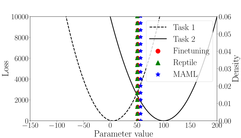
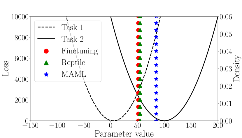
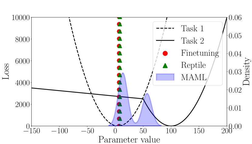
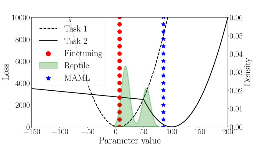
First, we study the behaviour of finetuning, Reptile, and MAML in two synthetic scenarios and , consisting of two tasks each. In this subsection, we use a slightly more abstract notion of tasks compared with the rest of the text, and define tasks purely abstractly by loss functions. These tasks can be considered the meta-train set, and the goal of the algorithms is to find good initialization parameters on this task distribution. We represent tasks by their loss landscape, which we have constructed by hand for illustrative purposes. In scenario , the two task loss landscapes are quadratic functions of a single parameter . More specifically, the losses for this scenario are given by and . In scenario , the first task loss landscape is the same while the second task represents a more complex function:
| (7) |
The respective algorithms train by sampling tasks in an interleaved fashion, and by adapting the parameter based on the loss landscape of the sampled task. We investigate the behaviour of Reptile and MAML when they make or task-specific adaptation steps. For this, we average the found solutions of the techniques over different runs with initial values that are equally spaced in the interval . We find that finetuning converges to the same point regardless of the initialization and is thus represented by a single vertical line. For Reptile and MAML, the found solution depends on the initialization, which is why we represent the found solution as a probability density. A Jupyter notebook for reproducing these results can be found on our GitHub page.
Based on the learning objectives of the techniques, we expect finetuning to settle for an initialization that has a good initial performance on both tasks (small loss values). Furthermore, we expect that MAML will pick any initialization point from which it can reach minimal loss on both tasks within steps. Reptile is expected to find a mid-way solution between finetuning and MAML.
The results of these experiments are displayed in Figure 1. In scenario (top figures), we see that both finetuning and Reptile prefer an initialization at the intersection of the two loss curves, where the initial loss is minimal. MAML, on the other hand, neglects the initial performance when and leans more to the right, whilst ensuring that it can reach the two optima within steps. The reason that it prefers an initialization on the right of the intersection is that the loss landscape of task 1 is steeper, which means that task adaptation steps will be larger. Thus, a location at the right of the intersection ensures good learning of task 2 and yields comparatively fast learning on the first task.
In scenario (bottom figures), the loss landscape of task 2 has a relatively flat plateau on the left-hand side. Because of this, finetuning and Reptile will be pulled towards the optimum (also the joint optimum) of the first task due to the larger gradients compared with the small gradients of the flat region of the second task when is small. The solution that is found by MAML when depends on the random initialization of the parameter, as can be seen in plot c). That is, when the random initialization is on the left of the plateau, MAML can not look beyond the flat region, implying that it will also be pulled towards the minimum of task 1. When , allowing the Reptile and MAML to look beyond the flat region, we see that Reptile either finds an initialization at (when the starting point is on the right-hand side of the plateau) or at the joint optimum at (when it starts with on the plateau). In the latter case, the post-adaptation performance of Reptile on both tasks is not optimal because it cannot reach the optimum of task 2. MAML, on the other hand, does not suffer from this suboptimality because it neglects the initial and intermediate performance and simply finds an initialization at from which it can reach both the optima of tasks 1 and 2.
5.2 Few-shot image classification
We continue our investigations by studying why MAML and Reptile can outperform finetuning in within-distribution few-shot image classification settings (see Section 3.2) when using a Conv-4 backbone. For these experiments, we use the -way -shot classification setting (see Section 3.2) on the miniImageNet (Vinyals et al., 2016; Ravi and Larochelle, 2017) and CUB (Wah et al., 2011) benchmarks. miniImageNet is a mini variant of the large ImageNet dataset (Deng et al., 2009) for image classification, consisting of colored images of size . The dataset contains 100 classes and 600 examples per class. We use the same train/validation/test class splits as in Ravi and Larochelle (2017). The CUB dataset contains roughly RGB images of birds from 200 species (classes). We use the same setting and train/validation/test class splits as in Chen et al. (2019).
Note that using real datasets entails that we move away from the abstract task definition as in the previous toy experiment, where the loss signal of the task was perfect. Instead, the loss signal is now approximated by sampling a finite set of data points for every task (for MAML and Reptile) or batch (for finetuning) and computing the performance of the methods on it.
For finetuning and MAML, we tune the hyperparameters on the meta-validation tasks using random search with a budget of 30 function evaluations for every backbone and dataset. We train MAML on tasks in the 1-shot setting and on tasks in the 5-shot setting, and validate its performance every tasks. The checkpoint with the highest validation accuracy is then evaluated on holdout test tasks. Similarly, finetuning is trained on batches of data from the training split when we evaluate it in the 1-shot setting and on batches when evaluating it in the 5-shot setting. Note that finetuning is trained on simple mini-batches of data instead of tasks consisting of a support and query set, and is later validated and tested on unseen validation and test tasks, respectively. In a similar fashion as for MAML, we validate its performance every batches. Due to the computational expenses, for Reptile, we use the best-reported hyperparameters and training iterations on 5-way 1-shot miniImageNet as found by Nichol et al. (2018). We use Torchmeta for the implementation of the data loaders (Deleu et al., 2019). We note that a single run of MAML and finetuning finish within one day, while Reptile finished within 4 days, perhaps due to the absence of parallelism in the implementation we used.
5.2.1 The role of the output layer
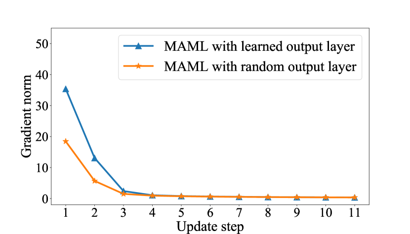
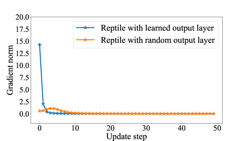
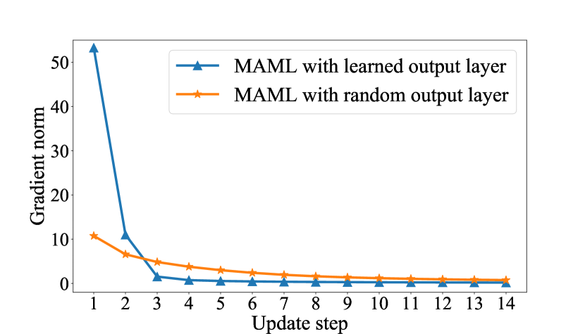
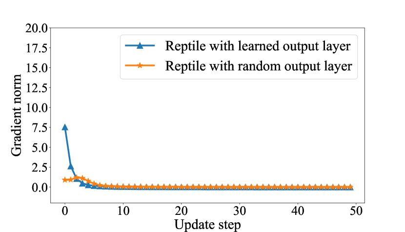
Here, we investigate whether the fact that MAML and Reptile reuse their learned output layer when learning new tasks alter their inner-learning behaviour and give them an advantage in performance compared with finetuning, which removes the learned output layer and replaces it with a randomly initialized one when learning a new task. In short, we study the role of the output layer on the performance and inner-loop adaptation behaviour of MAML and Reptile. For this, we perform meta-training for MAML and Reptile on 5-way 1-shot miniImageNet classification, and study the effect of replacing the learned output layer initialization weights with random weights on their ability to learn new tasks. Note that even though the weight initialization of the output layer may be random, it is still trained on the support sets of unseen tasks, therefore, finetuned to the task upon which it will be evaluated. Figure 2 displays the effect of replacing the output layer of the meta-learned weight initialization by MAML and Reptile meta-trained on 5-way 1-shot miniImageNet, with a randomly initialized one on the gradient norms during the inner-loop adaptation procedure. As we can see, the networks of the variants with a learned output layer receive larger gradient norms at the first few updates compared with the variants using a randomly initialized output layer, indicating that the learned output layer alters the learning behaviour of the algorithms. However, at the end of adaptation for a given task, the gradient norms are close to zero for both variants, indicating that both have converged to a local minimum. This implies that the learned initialization of the output layer has a distinct influence on the learning behaviour of new tasks. More specifically, using a learned output layer may aid in finding an initialization in the loss landscape that is sensitive to tasks and can be quickly adapted, explaining the larger gradient norms.
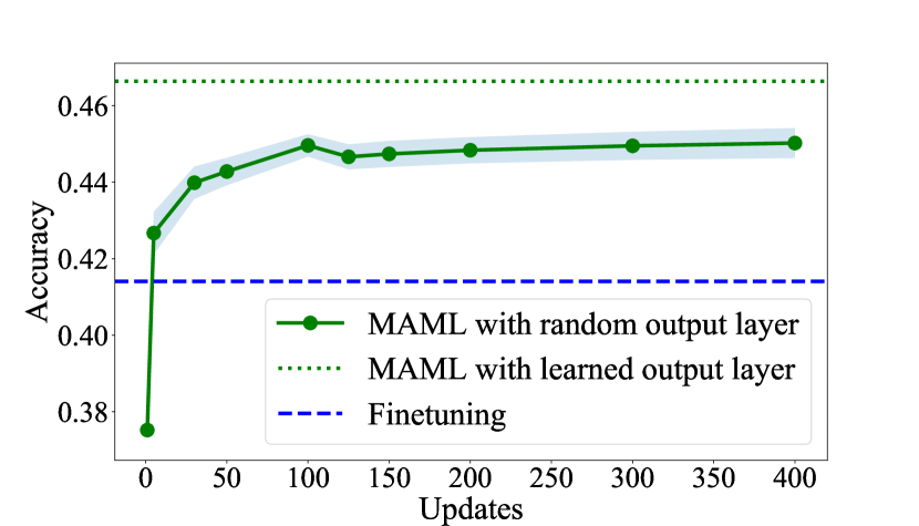
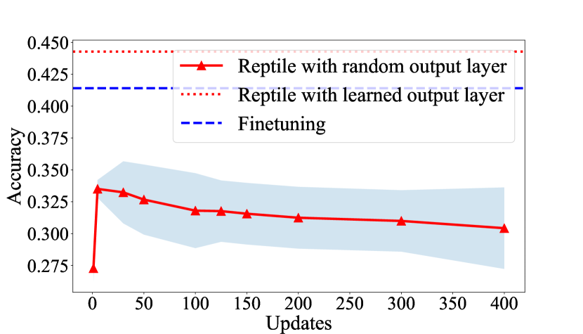
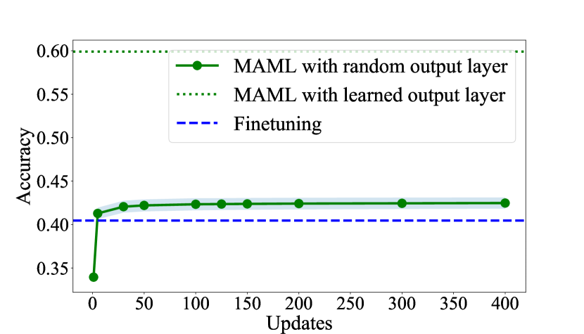
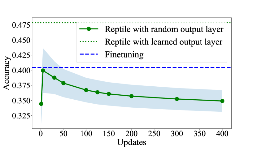
Next, we investigate whether reusing the learned output layers also leads to performance differences. For this, we investigate the influence of replacing the learned output layers in MAML and Reptile with randomly initialized ones when starting to learn new tasks on their learning performance for different numbers of update steps. The results are shown in Figure 3. As we can see, replacing the output layer with a random one leads to worse performance. Increasing the number of updates improves the performance for MAML, while the reverse is true for Reptile. In the end, the performance gap introduced by replacing the output layers with random ones is not closed, indicating that the output layers play an important role in successful inner-loop adaptation.
5.2.2 Specialization for robustness against overfitting
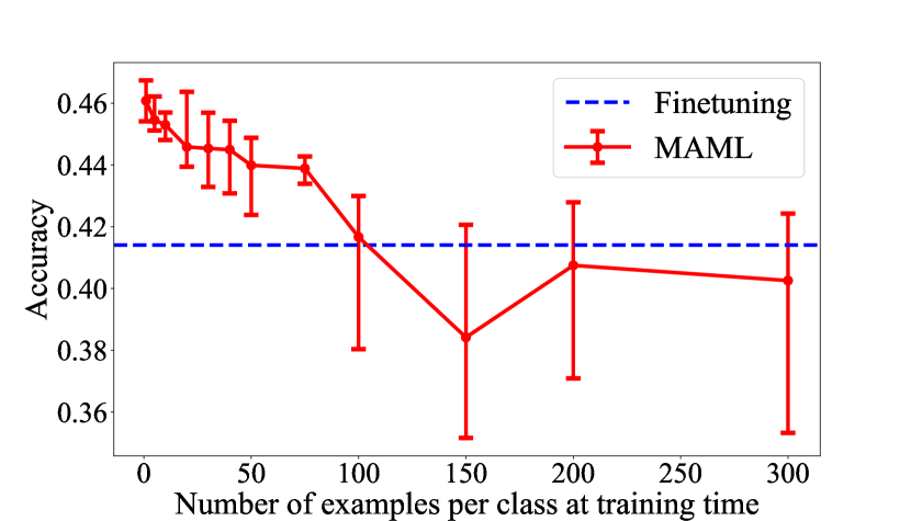
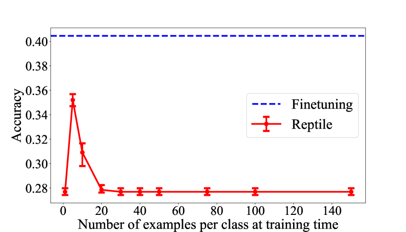
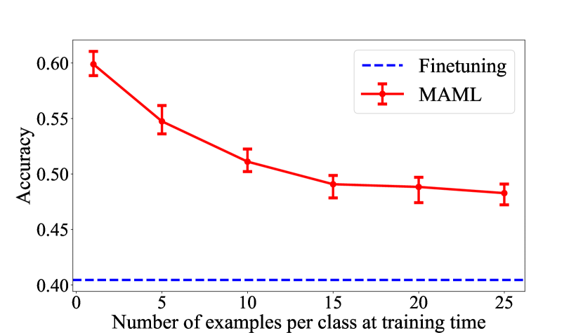
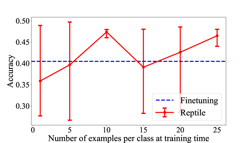
In this subsection, we investigate the influence of the level of data scarcity in the support set on the performance of MAML and Reptile. We hypothesize that both algorithms learn an initialization that is robust against overfitting when the number of examples in the support set per class () is small. This would imply that their performance would suffer when the number of examples in the support sets in training tasks is large due to the reduced need to become robust against overfitting, disabling the meta-learning techniques to become robust to overfitting during task-specific adaptation. We investigate this for 5-way miniImageNet image classification by varying the number of examples in the support set of meta-training tasks and measuring the performance on tasks with only one example per class (1-shot setting).
Figure 4 displays the results of these experiments. As we can see, there is an adverse effect of increasing the number of support examples per task on the final 1-shot performance of MAML. This shows that for MAML, it is important to match the training and test conditions so the initialization parameters can become robust against overfitting induced by data scarcity. In addition, we observe that Reptile is unstable due to its sensitivity to different hyperparameters on miniImageNet, even in the setting where . This is caused by the fact that Reptile is not allowed to sample mini-batches of data from the support set. Instead, we force it to use the full support set to investigate the effect of the number of support examples. When the number of examples is close to ten, which is the mini-batch size commonly used, as by the original authors (Nichol et al., 2018), there is a slight increase in performance for Reptile on miniImageNet, supporting the observation that it is sensitive to the chosen hyperparameters. On CUB, in contrast, we observe that the performance improves with the number of examples per class at training time, although the maximum number of examples investigated is 25 due to the fact that not every class has more examples than that. This illustrates that the sensitivity to hyperparameters depends on the chosen dataset.
5.2.3 Information content in the learned initializations
Next, we investigate the relationship between the few-shot image classification performance and the discriminative power of the learned features by the three techniques for different backbones (Conv-4, ResNet10, ResNet18 (He et al., 2015)).
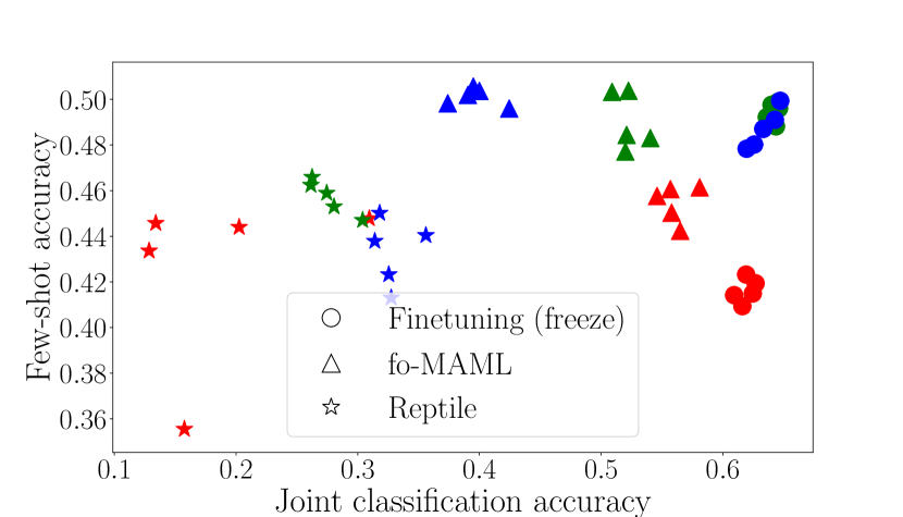
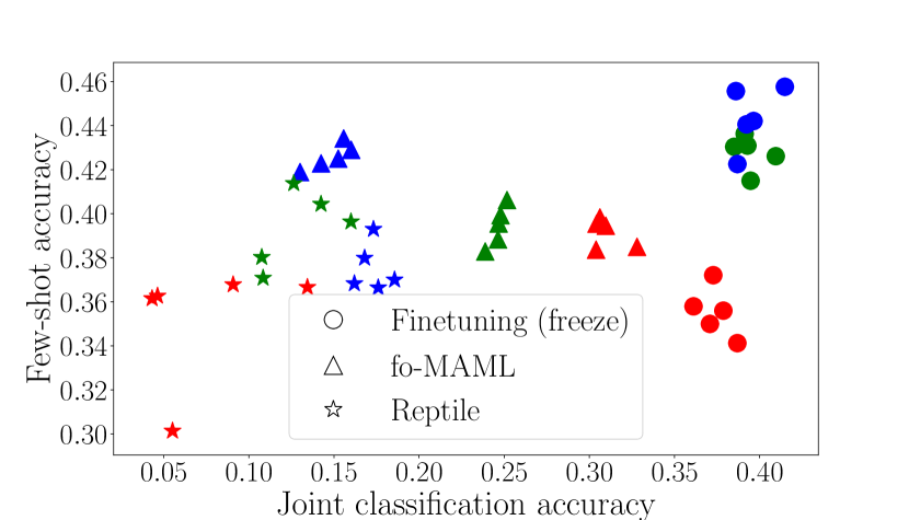
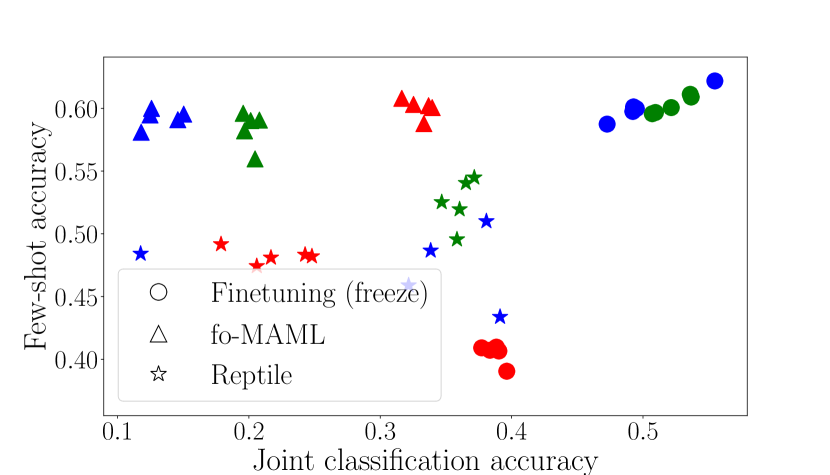
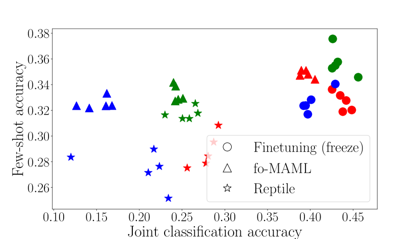
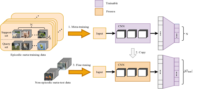
After deploying the three techniques on the datasets in a 5-way 1-shot manner, we measure the discriminative power of the learned initializations. Figure 5 visualizes this procedure for MAML and Reptile; finetuning follows a similar procedure. First, we extract the learned initialization parameters from the techniques. Second, we load these initializations into the base-learner network, freeze all hidden layers, and replace the output layer with a new one. The new output layer contains one node for every of the classes in the meta-test data. Third, we fine-tune this new output layer on the meta-test data in a non-episodic manner, which corresponds to regular supervised learning on the meta-test dataset. We use a 60/40 train/test split and evaluate the final performance on the latter. We refer to the resulting performance measure as the joint classification accuracy, which aims to indicate the discriminative power of the learned initialization, evaluated on data from unseen classes. Note that we use the expressions “discriminative power” and “information content” of the learned backbone synonymously.
MIN MIN CUB CUB CUB MIN Finetuning r=0.82, p=2e-4 r=0.71, p=3e-3 r=0.96, p=7e-9 r=0.28, p=0.31 MAML r=-0.77, p=8e-4 r=-0.85, p=6e-5 r=0.36, p=0.18 r=0.90, p=4e-6 Reptile r=0.27, p=0.3 r=0.50, p=0.06 r=0.3, p=0.28 r=0.31, p=0.27
The results of this experiment are shown in Figure 6. From this figure, we see that finetuning yields the best joint classification accuracy in all scenarios. From this figure, we see the following things.
-
•
The within-distribution few-shot learning performance is better than the out-of-distribution performance for all techniques
-
•
MAML achieves the best few-shot learning performance when using a shallow backbone (conv-4)
-
•
When the backbone becomes deeper, the features learned by MAML become less discriminative
-
•
Finetuning learns the most discriminative set of features for direct joint classification on a large set of classes
However, we note that the joint classification performance either weakly correlates or does not correlate with the few-shot learning performance across the different techniques. We note that these correlation patterns may be affected by the fact that we used the best-reported hyperparameters for Reptile for the Conv-4 backbone, while we also use ResNet-10 and ResNet-18 backbones (He et al., 2015) in different settings. For finetuning, however, we do observe an improvement in few-shot learning performance as the backbone becomes deeper.
Next, we investigate whether there are statistically significant relationships per technique between the joint classification accuracy and the few-shot performance. Table 2 displays the Pearson correlation and corresponding p-values for individual techniques for the experiment in Section 5.2.3. As we can see, there are strong and significant () correlations between the joint classification accuracy and the few-shot learning performance of finetuning in three settings. For MAML, there are strong negative correlations on miniImageNet and miniImageNet CUB, indicating that a lower joint classification accuracy is often associated with better few-shot learning performance. For Reptile, the correlations are non-significant and mild to weak.
6 Conclusion
In this work, we investigated 1) why MAML and Reptile can outperform finetuning in within-distribution settings, and 2) why finetuning can outperform gradient-based meta-learning techniques such as MAML and Reptile when the test data distribution diverges from the training data distribution.
We have shown how the optimization objectives of the three techniques can be interpreted as maximizing the direct performance, post-adaptation performance, and a combination of the two, respectively. That is, finetuning aims to maximize the direct performance whereas MAML aims to maximize the performance after a few adaptation steps, making it a look-ahead objective. Reptile is a combination of the two as it focuses on both the initial performance as well as the performance after every update step on a given task. As a result, finetuning will favour an initialization that jointly minimizes the loss function, whereas MAML may settle for an inferior initialization that yields more promising results after a few gradient update steps. Reptile picks something in between these two extremes. Our synthetic example in Section 5.1 shows that these interpretations of the learning objectives allow us to understand the chosen initialization parameters.
Our empirical results show that these different objectives translate into different learned initializations. We have shown that MAML and Reptile specialize for adaptation in low-data regimes of the training tasks distribution, which explains why these techniques can outperform finetuning as observed by Chen et al. (2019); Finn et al. (2017); Nichol et al. (2018), answering our first research question. Both the weights of the output layer and the data scarcity in training tasks play an important role in facilitating this specialization, allowing them to gain an advantage over finetuning.
Moreover, we have found that finetuning learns a broad and diverse set of features that allows it to discriminate between many different classes. MAML and Reptile, in contrast, optimize a look-ahead objective and settle for a less diverse and broad feature space as long as it facilitates robust adaptation in low-data regimes of the same data distribution (as that is used to optimize the look-ahead objective). This can explain findings by Chen et al. (2019), who show that finetuning can yield superior few-shot learning performance in out-of-distribution settings. However, we do not observe a general correlation between the feature diversity and the few-shot learning performance across finetuning, Reptile, and MAML.
Another result is that MAML yields the best few-shot learning performance when using the Conv-4 backbone in all settings. Interestingly, the features learned by MAML become less discriminative as the depth of the backbone increases. This may indicate an over-specialization, and it may be interesting to see whether adding a penalty for narrow features may prevent this and increase the few-shot learning performance with deeper backbones and in out-of-distribution settings, which has been observed to be problematic by Rusu et al. (2019) and Chen et al. (2019) respectively. As this is beyond the scope of our research questions, we leave this for future work. Another fruitful direction for future work would be to quantify the distance or similarity between different tasks and to investigate the behaviour of meta-learning algorithms as a function of this quantitative measure. An additional benefit of such a measure of task similarity would be that it could allow us to detect when a new task is within-distribution or out-of-distribution, which could inform the choice of which algorithm to use.
In summary, our results suggest that the answer to our second research question is that MAML and Reptile may fail to quickly learn out-of-distribution tasks due to their over-specialization to the training data distribution caused by their look-ahead objective, whereas finetuning learns broad features that allow it to learn new out-of-distribution concepts. This is supported by the fact that in almost all scenarios, there are statistically significant relationships between the broadness of the learned features and the few-shot learning ability for finetuning.
Acknowledgements
This work was performed using the compute resources from the Academic Leiden Interdisciplinary Cluster Environment (ALICE) provided by Leiden University, as well as the Dutch national e-infrastructure with the support of SURF Cooperative.
Declarations
Conflicts of Interest
Funding
Not applicable: no funding was received for this work.
Employment
All authors declare that there is no recent, present, or anticipated employment by any organization that may gain or lose financially through publication of this manuscript.
Interests
All authors certify that they have no affiliations with or involvement in any organization or entity with any financial interest or non-financial interest in the subject matter or materials discussed in this manuscript.
Compliance with Ethical Standards
Not applicable: this research did not involve human participants, nor did it involve animals.
Consent to participate
Not applicable.
Consent for publication
Not applicable: this research does not involve personal data, and publishing of this manuscript will not result in the disruption of any individual’s privacy.
Availability of data and material
Code availability
All code that was used for this research is made publicly available at https://github.com/mikehuisman/revisiting-learned-optimizers.
Authors’ contributions
MH has conducted the research presented in this manuscript. AP and JvR have regularly provided feedback on the work, contributed towards the interpretation of results, and have critically revised the whole.
All authors approve the current version to be published and agree to be accountable for all aspects of the work in ensuring that questions related to the accuracy or integrity of any part of the work are appropriately investigated and resolved.
Ethics approval
Not applicable.
References
- Brazdil et al. [2022] P. Brazdil, J. N. van Rijn, C. Soares, and J. Vanschoren. Metalearning: Applications to Automated Machine Learning and Data Mining. Springer, Cham, 2nd edition, 2022.
- Chen et al. [2019] W.-Y. Chen, Y.-C. Liu, Z. Kira, Y.-C. F. Wang, and J.-B. Huang. A closer look at few-shot classification. In International Conference on Learning Representations, ICLR’19, 2019.
- Collins et al. [2020] L. Collins, A. Mokhtari, and S. Shakkottai. Why does maml outperform erm? an optimization perspective. arXiv preprint arXiv:2010.14672, 2020.
- Deleu et al. [2019] T. Deleu, T. Würfl, M. Samiei, J. P. Cohen, and Y. Bengio. Torchmeta: A Meta-Learning library for PyTorch, 2019. URL https://arxiv.org/abs/1909.06576. Available at: https://github.com/tristandeleu/pytorch-meta.
- Deng et al. [2009] J. Deng, W. Dong, R. Socher, L.-J. Li, K. Li, and L. Fei-Fei. ImageNet: A Large-Scale Hierarchical Image Database. In Proceedings of the IEEE Conference on Computer Vision and Pattern Recognition, pages 248–255. IEEE, 2009.
- Finn et al. [2017] C. Finn, P. Abbeel, and S. Levine. Model-agnostic meta-learning for fast adaptation of deep networks. In Proceedings of the 34th International Conference on Machine Learning, ICML’17, page 1126–1135. PMLR, 2017.
- He et al. [2015] K. He, X. Zhang, S. Ren, and J. Sun. Delving deep into rectifiers: Surpassing human-level performance on imagenet classification. In Proceedings of the IEEE international conference on computer vision, pages 1026–1034, 2015.
- Hospedales et al. [2021] T. M. Hospedales, A. Antoniou, P. Micaelli, and A. J. Storkey. Meta-learning in neural networks: A survey. IEEE Transactions on Pattern Analysis & Machine Intelligence, 2021.
- Huisman et al. [2021] M. Huisman, J. N. van Rijn, and A. Plaat. A survey of deep meta-learning. Artificial Intelligence Review, 54(6):4483–4541, 2021.
- Huisman et al. [2022] M. Huisman, A. Plaat, and J. N. van Rijn. Stateless neural meta-learning using second-order gradients. Machine Learning, 111(9):3227–3244, 2022.
- Krizhevsky et al. [2012] A. Krizhevsky, I. Sutskever, and G. E. Hinton. ImageNet Classification with Deep Convolutional Neural Networks. In Advances in Neural Information Processing Systems 25, NIPS’12, pages 1097–1105, 2012.
- LeCun et al. [2015] Y. LeCun, Y. Bengio, and G. Hinton. Deep learning. Nature, 521(7553):436–444, 2015.
- Lee et al. [2019] K. Lee, S. Maji, A. Ravichandran, and S. Soatto. Meta-learning with differentiable convex optimization. In Proceedings of the IEEE Conference on Computer Vision and Pattern Recognition, pages 10657–10665, 2019.
- Mangla et al. [2020] P. Mangla, N. Kumari, A. Sinha, M. Singh, B. Krishnamurthy, and V. N. Balasubramanian. Charting the right manifold: Manifold mixup for few-shot learning. In Proceedings of the IEEE/CVF Winter Conference on Applications of Computer Vision, pages 2218–2227, 2020.
- Mnih et al. [2015] V. Mnih, K. Kavukcuoglu, D. Silver, A. A. Rusu, J. Veness, M. G. Bellemare, A. Graves, M. Riedmiller, A. K. Fidjeland, G. Ostrovski, et al. Human-level control through deep reinforcement learning. Nature, 518(7540):529–533, 2015.
- Nichol et al. [2018] A. Nichol, J. Achiam, and J. Schulman. On First-Order Meta-Learning Algorithms. arXiv preprint arXiv:1803.02999, 2018.
- Raghu et al. [2020] A. Raghu, M. Raghu, S. Bengio, and O. Vinyals. Rapid Learning or Feature Reuse? Towards Understanding the Effectiveness of MAML. In International Conference on Learning Representations, ICLR’20, 2020.
- Ravi and Larochelle [2017] S. Ravi and H. Larochelle. Optimization as a Model for Few-Shot Learning. In International Conference on Learning Representations, ICLR’17, 2017.
- Rusu et al. [2019] A. A. Rusu, D. Rao, J. Sygnowski, O. Vinyals, R. Pascanu, S. Osindero, and R. Hadsell. Meta-learning with latent embedding optimization. In International Conference on Learning Representations, ICLR’19, 2019.
- Schaul and Schmidhuber [2010] T. Schaul and J. Schmidhuber. Metalearning. Scholarpedia, 5(6):4650, 2010.
- Schmidhuber [1987] J. Schmidhuber. Evolutionary principles in self-referential learning, or on learning how to learn: the meta-meta-… hook. Master’s thesis, Technische Universität München, 1987.
- Silver et al. [2016] D. Silver, A. Huang, C. J. Maddison, A. Guez, L. Sifre, G. Van Den Driessche, J. Schrittwieser, I. Antonoglou, V. Panneershelvam, M. Lanctot, et al. Mastering the game of go with deep neural networks and tree search. Nature, 529(7587):484–489, 2016.
- Snell et al. [2017] J. Snell, K. Swersky, and R. Zemel. Prototypical Networks for Few-shot Learning. In Advances in Neural Information Processing Systems 30, NIPS’17, pages 4077–4087. Curran Associates Inc., 2017.
- Thrun [1998] S. Thrun. Lifelong Learning Algorithms. In Learning to learn, pages 181–209. Springer, Boston, MA, 1998.
- Tian et al. [2020] Y. Tian, Y. Wang, D. Krishnan, J. B. Tenenbaum, and P. Isola. Rethinking few-shot image classification: a good embedding is all you need? arXiv preprint arXiv:2003.11539, 2020.
- Vinyals et al. [2016] O. Vinyals, C. Blundell, T. Lillicrap, K. Kavukcuoglu, and D. Wierstra. Matching Networks for One Shot Learning. In Advances in Neural Information Processing Systems 29, NIPS’16, pages 3637–3645, 2016.
- Wah et al. [2011] C. Wah, S. Branson, P. Welinder, P. Perona, and S. Belongie. The Caltech-UCSD Birds-200-2011 Dataset. Technical Report CNS-TR-2011-001, California Institute of Technology, 2011.
- Wu et al. [2016] Y. Wu, M. Schuster, Z. Chen, Q. V. Le, M. Norouzi, W. Macherey, M. Krikun, Y. Cao, Q. Gao, K. Macherey, J. Klingner, A. Shah, M. Johnson, X. Liu, Łukasz Kaiser, S. Gouws, Y. Kato, T. Kudo, H. Kazawa, K. Stevens, G. Kurian, N. Patil, W. Wang, C. Young, J. Smith, J. Riesa, A. Rudnick, O. Vinyals, G. Corrado, M. Hughes, and J. Dean. Google’s Neural Machine Translation System: Bridging the Gap between Human and Machine Translation. arXiv preprint arXiv:1609.08144, 2016.
- Yang et al. [2021] S. Yang, L. Liu, and M. Xu. Free lunch for few-shot learning: Distribution calibration. In International Conference on Learning Representations, ICLR’21, 2021.