Recovering 21cm monopole signals without smoothness

Abstract

We expect the monopole signal at the lowest frequencies below $100\,$MHz to be composed to two components: the deep Rayleigh-Jeans tail of the cosmic microwave background and two distinct features: the dark ages trough at $\sim 17\,$MHz and the cosmic dawn trough at $\sim 75\,$Mhz. These are hidden under orders of magnitude brighter foregrounds whose emission is approximately a power-law with a spectral index $\approx-2.5$. It is usually assumed that monopole signals of interest are separable from foregrounds on the basis of spectral smoothness. We argue that this is a difficult approach and likely impossible for the Dark Ages trough. Instead, we suggest that the fluctuations in the foreground emission around the sky should be used to build a model distribution of possible shapes of foregrounds, which can be used to constrain presence of a monopole signal. We implement this idea using normalizing flows and show that this technique allows for efficient unsupervised detection of the amplitude, width and center of the Dark Ages trough as well as Rayleigh-Jeans tail of the cosmic microwave background for a sufficiently sensitive experiment. We discuss the limitations of the inherent assumptions in this method and the impact on the design of future low-frequency experiments.

1 Introduction

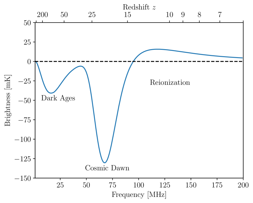
After the epoch of recombination at redshift around $z\sim 1150$ and before the universe is completely reionized at redshifts $z\lesssim 6$, the universe is filled with neutral hydrogen, which is predicted to be observable against cosmic microwave background emission at radio frequencies below $\nu\lesssim 200\,$MHz. This period in the evolution of the Universe can be approximately divided into two chapters: the Dark Ages, before the advent of first stars, where the neutral hydrogen is largely in its pristine primordial state and the Cosmic Dawn, when first sources light up on the sky and start to illuminate and photo-ionize the neutral primordial medium eventually leading to reionization. Each episode is associated with a mean absorption profile as illustrated in Figure 1. For an in-depth discussion of these effects see [Pritchard and Loeb (2012)], [Furlanetto (2019)]. Measurements of either of these absorption signals would be transformative for understanding of the evolution of our Universe.

The Dark Ages absorption trough is of depth $\sim 40\,$mK and is centered at around $\nu\sim 17\,$MHz and has a width of $\Delta\nu\sim 8\,$MHz. Its precise shape can be calculated from the first principles assuming only the standard cosmology (i.e. linearized general relativity, thermodynamics and atomic physics, but not astrophysics) and is very sensitive to any injection or sink of energy in the primordial medium. It has never been measured and will very likely require a space-based observatory.

The Cosmic Dawn absorption trough is of depth $\sim 140\,$mK and is centered at around $\nu\sim 75\,$MHz and has a width of $\Delta\nu\sim 10\,$MHz. Its shape is very sensitive to the physics of first stars and the process of reionization. There is an active experimental program in attempts to constrain this signal. There are tentative detections by the EDGES team (Bowman et al., 2018) at $78\pm 1\,$MhZ for a symmetric U-shaped profile of amplitude $500^{+500}_{-200}\,$mK, which are disputed by others, like the SARAS3 team Singh et al. (2021), either as modelling or as instrumental systematics (Hills et al., 2018; Bradley et al., 2019).

Finally, the same frequencies of interest should also contain the deep Rayleigh-Jeans tail of the cosmic microwave background. Detection of this background would be of interest from both theoretical perspective (Pospelov et al., 2018; Caputo et al., 2023; Acharya and Chluba, 2023) as well as clarification on the recent excess monopole radiation at the very low frequencies (Dowell and Taylor, 2018; Fixsen et al., 2011).

The main difficulty in experimental detection of the signal is the existence of bright foregrounds. These foregrounds are orders of magnitude brighter and we do not have an obvious a-priori model to separate them from the signal of interest. So far, the major proposed method has been to separate the foreground from the signal of interest based on foreground smoothness. We will argue in Section 2 that there is a certain element of wishful thinking involved in this approach. In Section 3 we will propose a different method with its own unique assumptions. In Sections 4 and 5 we discuss its implementation and results when applied to synthetic datasets. We conclude in Section 6.

Figure 1: Evolution of the 21cm cosmic hydrogen signal with redshift and frequency

2 Separating foregrounds

Separating foregrounds from signal is the foundational problem of the 21 cm cosmology. We can write the sky temperature in direction $\hat{\mathbf{x}}$ and frequency $\nu$ as

$$T(\hat{\mathbf{x}},\nu)=T_{\rm s}(\nu)+T_{\rm fg}(\hat{\mathbf{x}},\nu)=T_{\rm s}(\nu)+\bar{T}_{\rm fg}(\nu)+\Delta T_{\rm fg}(\hat{\mathbf{x}},\nu),$$ (1)

where we have split the signal into monopole signal of interest $T_{\rm s}(\nu)$ and the foreground temperature $T_{\rm fg}(\hat{\mathbf{x}},\nu)$. In this treatment, we ignore fluctuations in the signal and focus solely on the monopole signal. The fluctuations in foreground are typically larger order of magnitude in brightness as the signal. We further split them into the foregrounds monopole $\bar{T}_{\rm fg}(\nu)$ and variations around this mean $\Delta T_{\rm fg}(\hat{\mathbf{x}},\nu)$. By definition then, these fluctuations must average to zero $\left<\Delta T_{\rm fg}(\hat{\mathbf{x}},\nu)\right>_{\hat{\mathbf{x}}}=0$, where the average is defined as usual over a sufficiently large observational patch.

From now on, we will drop the explicit frequency dependency in our notation and note that our measurements have an implicit frequency dependency with considerable dimensionality (i.e. 50 or so bins in frequency). We will still include dependency in spatial variations explicitly to distinguish between monopoles (which are functions of just frequency) and quantities that vary both with frequency and position on the sky.

It is obvious from the above that $T_{\rm s}$ and $\bar{T}_{\rm fg}$ are perfectly degenerate in any observation, unless we make further assumptions that enable separation.

2.1 Smoothness separation

The usual assumption is that we can separate the foreground emission from the signal by application of smoothness in the frequency direction. The foregrounds are smooth, while the signal is largely not. Schematically, high-pass filter applied to the $T_{\rm s}+\bar{T}_{\rm fg}$ will result in $\approx\bar{T}_{\rm fg}$. This has lead to heroic attempts by experimentalists to ensure exquisite smoothness of spectral response of their instruments. It also led to development of several interesting formalisms in trying to capture what is really meant by spectral smoothness (Sathyanarayana Rao et al., 2015; Bevins et al., 2020).

This approach is based on intuition from spectroscopy, where the equivalent line widths can be measured quite accurately, even for spectra where broadband spectro-photometry is quite poor. The idea is that we have a narrow feature on top of some smoothly varying background. As long as the feature is more pronounced than the typical variation of the background over the width of the feature, one should be able to extract it cleanly. To put this on a more quantitative footing, assume we have a slowly varying background $B(\nu)$ of typical amplitude $A$ with an absorption or emission feature of amplitude $S$ imprinted over some frequency range $\Delta\nu$. Typical variation of the background over the width of the feature will go as

$$\Delta B\sim\frac{\Delta\nu}{\nu}A$$ (2)

(i.e. for locally power-law shaped backgrounds, it will be of this form with the spectral index as a prefactor.). This will also determine a typical uncertainty in the background determination over the width the feature. In order to cleanly separate the feature, we require that this a subdominant uncertainty

$$\frac{S}{A}>\frac{\Delta\nu}{\nu}.$$ (3)

For Cosmic Dawn signal, $S/A\sim 10^{-3}$ and for the Dark Ages signal $S/A\sim 10^{-5}$. On the other hand, we have $\Delta\nu/\nu\sim 0.1$ and $\sim 1$ respectively. We see that this smoothness separation condition is violated already for the cosmic dawn feature. It is therefore not surprising that the statistical significance of this detection has been discussed in the literature (Hills et al., 2018; Bradley et al., 2019). If they were looking for a truly narrow spectral feature, the significance would have been much less modelling dependent. The condition is even more badly violated for the Dark Ages feature.

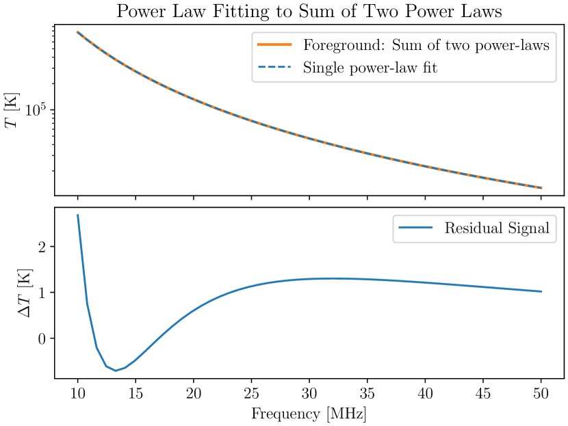
To illustrate this point further on a concrete example, we consider the following toy model: there are two patches of the sky, each emitting a pure power-law emission with spectral indices -2.54 and -2.56 respectively and contributing equally to the total emission. When fit with a single power-law, the residuals show a clear fake news trough. This is illustrated in the Figure 2. Clearly, in reality, with multiple power-law like contributions to the signal, the residuals can be either full of fake structure (if the fitting model is insufficiently flexible) or completely gone if the model is overly flexible. Fundamentally, unless one has a physical model of the sky that is accurate at the $10^{-5}$ level, there is no way to distinguish between over and under-fitting regardless of how many Monte-Carlos simulations does one run.

Figure 2: A toy example: A sum of two power laws with spectral indices of -2.54 and -2.56 (orange) is fit with a single power law (blue dashed). Residuals are shown in the bottom panel.

The situation is somewhat less drastic in the case of Cosmic Dawn, since the foregrounds are both less bright and the peak sharper. At the same time, the sky might also be more complicated than we think it is, so smoothness-based separation techniques remain a challenge.

2.2 Explicit foreground modelling

An alternative from smoothness based separation is to involve building a model of the foreground degrees of freedom. Such model can have a large number of free parameters that can be determined from the data, but in this approach the functional form the of the model is determined in advance or derived from a large set of realistic simulations called training datasets in this context. See Tauscher et al. (2018); Bassett et al. (2021) for examples of this approach in action. However, to reach precision required to subtract the foregrounds at $10^{-4}$ to $10^{-6}$ level required by the data is a daunting task that will likely require a very large parameters, perhaps exceeding a number that can be efficiently sampled using traditional Monte Carlo Markov Chain approaches.

2.3 Data driven foreground modelling

An alternative possibility is to infer the model for the foregrounds from the data itself. Any variations on the sky from one point to another, at least in the limit of an ideal instrument, are caused by the foreground variations and not the monopole component. Given a model of these variations and their relation with the foreground-only monopole, we can then use the model to constrain the presence of the non-foreground monopole.

The approach we take in this paper is to replace the assumption of smoothness with the assumption that the foreground monopole $\bar{T}_{\rm fg}$ is drawn from the same distribution as $\Delta T_{\rm fg}$. In other words, if $\mathcal{F}$ is the set of all possible deviations from the mean foreground, i.e. $\Delta T_{\rm fg}(\hat{\mathbf{x}})\in\mathcal{F}$ for any $\hat{\mathbf{x}}$, then $\bar{T}_{\rm fg}\in\mathcal{F}$. This is admittedly a strong assumption, but it is rooted in the physical intuition that foreground generating process is local. As an example, consider a sky that is generated as a combination of two power laws, as it was discussed in our toy example earlier (see Figure 2)

$$T_{\rm toy}(\hat{\mathbf{x}})=\alpha(\hat{\mathbf{x}})\left(\frac{T}{T_{A}}\right)^{-2.54}+(1-\alpha(\hat{\mathbf{x}}))\left(\frac{T}{T_{B}}\right)^{-2.56}$$ (4)

where $\alpha$ varies between $0$ and $1$ across the sky. In this case, the set $\mathcal{F}$ is composed of combination of power laws with exponents $-2.54$ and $-2.56$ and indeed $\bar{T}_{\rm fg}$ is in $\mathcal{F}$, while some general function of temperature is not.

Of course, it is not too hard to find counter-examples. The canonical example is to assume that there is some truly constant component to the foreground. But if there is some process happening in the universe that is producing foreground radiation, then the same process occurring at a larger distance would scale all components in flux and so making any constant contribution appear to vary. Another option is that fluctuations around the mean are much less than the mean itself, which is violated by simply looking at the orders of magnitude over which foreground signal varies across the galactic plane. In short, counter examples are typically inconsistent with the large variations in temperature across the sky, the locality assumption or the effective translational invariance assumption (the same processes occur at different distances from the observer).

In the following section we will develop a probabilistic framework for constraining the signal of interest $T_{\rm s}$ based off a generative model for $\mathcal{F}$ of the foregrounds.

3 Method

For a start, we assume a perfect instrument without any calibration errors or gain fluctuations. In this case, assuming some data from the sky $T(\hat{\mathbf{x}})$, we can calculate a monopole $T_{m}=\left<T(\hat{\mathbf{x}})\right>=\bar{T}_{\rm fg}+T_{\rm s}$ and fluctuations $\Delta T_{\rm fg}(\hat{\mathbf{x}})=T(\hat{\mathbf{x}})-T_{m}$.

A careful reader might immediately protest that data from the sky $T(\hat{\mathbf{x}})$ depend on the shape of the telescope’s beam. This is of course true, but crucially, the contribution from the monopole signal is independent of the shape of the beam (assuming it is correctly calibrated). Therefore, for the two different beams, the statistical properties of the foregrounds will be different, but since we self-calibrate them, this does not matter.

We then build a probabilistic model for the distribution of foreground fluctuations based on the samples $\Delta T_{\rm fg}(\hat{\mathbf{x}})$ across the sky. This model, essentially, is the likelihood function $P_{\rm fg}(T)$, which returns the likelihood that the given $T$ is drawn from the same distribution as $\Delta T_{\rm fg}$. Using our assumption that $\bar{T}_{\rm fg}$ is drawn from this distribution, we can write the likelihood of the signal of interest being present in the observed monopole $P(T_{\rm s}|T_{m})=P(T_{\rm s}|\bar{T}_{\rm fg}+T_{\rm s})$ in terms of the likelihood of the foreground model $P_{\rm fg}(T_{m}-T_{\rm s})$

$$P(T_{\rm s}|T_{m})\propto P_{\rm fg}(\bar{T}_{\rm fg})=P_{\rm fg}(T_{m}-T_{\rm s})$$ (5)

i.e. for any candidate $T_{\rm s}$, we can ask our probability function if the required $\bar{T}_{\rm fg}=T_{m}-T_{\rm s}$ is drawn from the foreground model. When the correct template signal of interest $T_{\rm s}$, with the right amplitude, width, etc., is subtracted from the overall monopole we are left with the foreground-only signal thereby assigning it a high likelihood by the foreground model. We have thus constructed a probability for $T_{\rm s}$.

Our implementation proceeds as follows. We first calculate the PCA basis of $\Delta T_{\rm fg}$ and then rotate the full set of $\Delta T_{\rm fg}$ into it. We then apply normalizing flow transformation, to map these vectors into a Gaussian distribution. By using appropriate Jacobian this now provides a probabilistic model for $\Delta T_{\rm fg}$, which we can use in a probabilistic model for $T_{s}$ in Equation (5).

4 Synthetic Data and Implementation Details

4.1 ULSA maps and model observations

To generate our synthetic data we use the Ultra Low-wavelength Sky with Absorption (ULSA) model from Cong et al. (2021). The ULSA model is the current state-of-the-art model for the low-frequency sky. It is anchored in the high frequency data, most importantly the Haslam 402 MHz map, and is valid down to $\sim 1$ MHz. It features direction and frequency dependent spectral indices and it takes into account free-free absorption by thermal electrons in the galaxy. The free-free absorption from the galaxy’s warm ionized medium causes a notable turnover effect in the $\lesssim 10$Mhz frequency range, a significant departure from the power-law radio background model.

While it is known that the ULSA map is likely not a fully accurate description of the reality, since it is inconsistent with some measurements, it currently offers the highest level of realism. It is sufficiently complex to be unlikely to give misleadingly optimistic results.

We generate maps with the HEALPix (Górski et al., 2005) resolution NSIDE =128 and with enabled direction-dependent spectral index using the code provided with the paper. We sample frequencies in 1MHz bins in the range 1-50MHz.

To observe these maps, we assume Gaussian beams with $\sigma=2^{\circ}$, $4^{\circ}$ and $6^{\circ}$ at $10\,$MHz. In the frequency direction we either keep the beam size constant (achromatic) or scale it with inverse of the observation frequency (chromatic). We will refer to beams by their size at $10\,$MHz and chromaticity. These are again not very realistic, but sufficient for our exploratory investigations, since they do mix several individual pixels of the source ULSA map into an observation spectrum. In particular, we wanted to understand how much impact will beam chromaticity have on our ability to separate foregrounds.

Finally, in all our investigations we remove the very bright regions around the galactic plane by imposing the galactic cut of $\pm 20^{\circ}$ in galactic latitude. We have observed that including galaxy in the data severely limits our ability to detect the signal, but also that the precise size of galactic cut is not crucial.

4.2 Rotation into PCA basis

Figure 3: This figure shows the separation of foregrounds and signal in different spaces. Top Left: separation in the original frequency space using an achromatic 2 degree beam. The blue distribution violins and the solid line describe the foreground signal distribution and mean (on the cut sky), the green line denotes the CMB signal and the orange solid line denotes the Dark Ages signal. Note the extremely large dynamic range on the vertical axis. Top Right: The amplitude of the same signals in the foreground PCA basis. Far from the galactic center, the first ten principal components are capable of absorbing 8 orders of magnitude in signal. The brown solid line denotes the RMS of the corresponding eigenmode. Bottom Panel Signal amplitudes scaled by the RMS of the corresponding eigenmode. The basis vectors have been multiplied by $-1$ to make all the Dark Ages contribution positive.

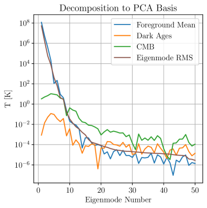
We start our analysis by taking the foreground fluctuation vector at each point $\Delta T_{\rm fg}(\hat{\mathbf{x}})=T(\hat{\mathbf{x}})-\bar{T}_{\rm fg}$ and rotating it into its principal component basis in the frequency space and further dividing it by the root-mean-square of variance in each basis direction. In other words, for each direction on the sky, we have replaced description of the data from a set of power spectrum measurement by the same number of component amplitudes with unit variance. The indices depend on the bases and thus dependent on the beam size and its chromaticity. These component numbers are also spatially correlated on short scales following the correlations of the parent frequency space description.

These is no loss of information in this rotation (as it is fully invertable), but it makes the subsequent normalizing flow process considerably more numerically robust. We have also found that naive application of principal component analysis is numerically unstable due to the very large dynamic range of data and therefore we implement this rotation using the singular vector decomposition approach. Further discussion of this issue can be found in the Appendix A

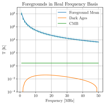
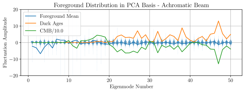
In Figure 3 we show how the signal looks like in the original space and in the PCA foreground eigenspace. In the top panel we see the many orders of magnitude that separate the signal of interest from the dark ages signal. The middle panel demonstrates that the first 20 or so eigen-modes absorb majority of the foreground complexity and that signal of interest does ”stick out” from the foregrounds for the sufficiently high order components. Note that this plot suppresses the cross-correlations between the foreground components which also ultimately help in identifying the signal of interest over the foreground distribution.

4.3 Building $P_{\rm fg}$ using Normalizing Flows

We proceed to model the foreground fluctuations in the PCA space using the Sliced Iterative Normalizing Flow (SINF) implementation of the Normalizing Flow model developed in Dai and Seljak (2021). The algorithm is stable, fast to train and performs well on small datasets for density estimation and out-of-distribution detection. For a given beam, we subsample the points for efficiency and use a randomly chosen $80\%$ of these points to train the model, and the rest for validation.

After training, the model learns several thousand layers of an affine transformation $\mathcal{N}=\{\mathcal{N}_{i}\}:\mathbb{R}^{n}\rightarrow\mathbb{R}^{n}$ to map the input distribution to a Gaussian. The log likelihood for any trial vector $\bar{T}_{\rm fg}$ can then be found as the usual change of variables given by the sum of the Gaussian log likelihood with the log Jacobian $\mathcal{J}$ of the transformation

$$\log P_{\rm fg}(\bar{T}_{\rm fg})=\log P(\mathcal{N}(\bar{T}_{\rm fg}))+\log\mathcal{J}$$ (6)

The SINF engine has several tunable parameters that regularize the normalizing flow to reduce overfitting and improve performance (see Eq. 13 in Dai and Seljak (2021)). We set these parameters to heavily regularize the data to avoid overfitting, which comes at the cost of slow training and a large number of iterations required for convergence. However, we feel this is required since overfitting is an important issue to mitigate in any distribution modelling task.

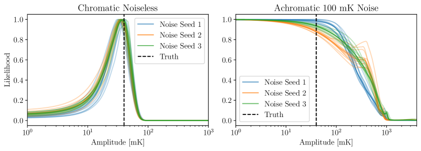
The SINF engine is inherently stochastic under the hood. While the results should not be affected by this, we find a very weak variance across runs on identical training data. This is elaborated in Appendx B

4.4 Multiscale fits

In our default implementation any scale-dependent information in the foregrounds is lost due to randomization, which is clearly sub-optimal. In order to bring in the scale dependence, we consider beams of different scales at the same spatial positions. Note that these do not in general correspond to a new physical beams, since fine resolution data can always be aggregated into coarser resolution.

In this preliminary work we consider 4^∘ and 6^∘ degree beams in addition to 2^∘ beams. Our data vector is then formed by concatenating the data from the 2^∘ beam with difference between 4^∘ and 2^∘ beams leading to data vectors $2\times 50$ elements long and additionally adding difference between 6^∘ and 4^∘ leading to data vectors that are $3\times 50$ elements long. We refer to these as $2^{\circ}+4^{\circ}$ and $2^{\circ}+4^{\circ}+6^{\circ}$ fits. In principle, we could equivalently simply concatenate the the data vectors at differing resolutions, but we have found the differencing procedure to be numerically stabler.

After generating such vectors, we proceed by calculating the new PCA basis for the full sized vectors and then use the normalizing flows in that corresponding PCA bases. The monopole signal in this space is given by the monopole signal concatenated with zeroes, since the monopole signal is independent of the beam shape and is simply subtracted.

We have tested the impact of throwing away the least important PCA components and found that while there was some variation in the results, there we no clear advantages or disadvantages in doing so.

4.5 CMB Signal Model

In order to test our method, we have considered a model with free CMB temperature. This model is trivial, it is just a frequency independent constant $T_{\rm CMB}(\nu)=2.718$. The reason for this parameterization is that it allows us to ask just how sensitive a putative futuristic experiment would be to the CMB temperature deep in the Rayleigh-Jeans limit. At the same time, it would allow us to tie the instrument’s calibration against a very robust CMB as a baseline.

The constant CMB temperature in frequency space translates to a non-trivial vector in the foreground PCA basis which, in comparison with the Dark Ages signal, is a much stronger monopole signal as can be seen in Fig. 3

4.6 Dark Ages Signal Model

It is clear from the Figure 3 that some linear combinations of the Dark Ages signal are forever lost to foregrounds. No method can therefore recover an unbiased shape of the Dark Ages signal. The only sensible approach in that case is to ask if one model of the Dark Ages signal is more likely than the other. We therefore build a phenomenological 3-parameter Dark Ages as follows. We start by the default Dark Ages monopole model as predicted by the ARES software package Mirocha (2014). In order to avoid method latching on low-frequency part of the brighter cosmic dawn peak, we have manually modified model so that it gracefully approaches zero at 50MHz by matching first and second derivatives as 32 MHz. We then scale this model in amplitude, position and width:

$$T_{\rm DA}(\nu,A,\nu_{c},\Delta\nu)=\frac{A}{A_{0}}T_{\rm ares}\left(\nu_{c0}+(\nu-\nu_{c})\frac{\Delta\nu}{\Delta\nu_{0}}\right)$$ (7)

where $A_{0}=40\,$mK, $\nu_{c0}=16.4\,$Mhz and $\Delta\nu_{0}=14\,$Mhz are (defined to be) values of amplitude, through position and width for the nominal model.

4.7 Likelihood analysis

Our model has three degrees of freedom and therefore the likelihood analysis can be done by brute-force evaluation on 3 sufficiently fine 3D grid. After we evaluate likelihood on a regular grid, we use the standard python MCMC package corner to plot and calculate marginalised constraints by assigning sample weights proportional to their likelihood.

When we have sufficient signal-to-noise we fit for all three parameters (amplitude, through position and through) width. Later when we explore the effects of the noise, we calculate exclusion limits by fitting the amplitude parameter only.

5 Results

In Table 1 we show a big compendium of results for the various tests that we have performed. The top line shows the ground truth. When the signal-to-noise was sufficient to measure the signal amplitude, we have performed the full 3 parameter fits. When the data is consistent with zero amplitude, the with and position become unconstrained and therefore we have only fitted for the amplitude parameter and reported the 95% upper limit.

5.1 Results in an idealistic case

Case	$A$ [mK]	$\Delta\nu$ [MHz]	$\nu_{c}$ [MHz]
Truth	40	14	16.4
Noiseless
Achromatic Beam:
$2^{\circ}$	$40.816^{+1.633}_{-1.306}$	$14.143^{+0.163}_{-0.082}$	$16.298^{+0.122}_{-0.122}$
$4^{\circ}$	$39.837^{+0.980}_{-0.980}$	$14.056^{+0.051}_{-0.031}$	$16.385^{+0.031}_{-0.031}$
$6^{\circ}$	$38.122^{+0.816}_{-0.816}$	$14.056^{+0.041}_{-0.031}$	$16.346^{+0.026}_{-0.031}$
$2^{\circ}+4^{\circ}$	$39.510^{+2.286}_{-2.286}$	$14.276^{+0.143}_{-0.184}$	$16.298^{+0.122}_{-0.163}$
$2^{\circ}+4^{\circ}+6^{\circ}$	$40.408^{+0.490}_{-0.327}$	$14.036^{+0.041}_{-0.020}$	$16.390^{+0.020}_{-0.061}$
Chromatic Beam:
$2^{\circ}$	$25.949^{+18.872}_{-18.872}$	$14.556^{+0.741}_{-0.667}$	$16.078^{+0.775}_{-0.620}$
$4^{\circ}$	$29.460^{+10.361}_{-9.066}$	$14.429^{+0.327}_{-0.327}$	$16.112^{+0.245}_{-0.286}$
$6^{\circ}$	$37.875^{+7.596}_{-6.330}$	$14.224^{+0.245}_{-0.163}$	$16.235^{+0.122}_{-0.204}$
$2^{\circ}+4^{\circ}$	$37.143^{+13.469}_{-9.796}$	$14.251^{+0.463}_{-0.206}$	$16.351^{+0.261}_{-0.229}$
$2^{\circ}+4^{\circ}+6^{\circ}$	$38.857^{+2.939}_{-2.612}$	$14.092^{+0.082}_{-0.061}$	$16.349^{+0.061}_{-0.082}$
Noise level
$2^{\circ}+4^{\circ}+6^{\circ}$
Achromatic
0.01mK	$39.510^{+0.980}_{-0.980}$	$14.046^{+0.051}_{-0.041}$	$16.369^{+0.020}_{-0.041}$
0.1mK	$37.866^{+5.338}_{-4.448}$	$14.143^{+0.245}_{-0.204}$	$16.420^{+0.163}_{-0.163}$
1mK	$<61.32$
100mK	$<129.760$
Chromatic $2^{\circ}+4^{\circ}+6^{\circ}$
0.01mK	$42.109^{+5.491}_{-5.491}$	$14.173^{+0.184}_{-0.143}$	$16.308^{+0.102}_{-0.082}$
0.1mK	$<77.55$
1mK	$<247.22$
100mK	$<2612.16$
$2^{\circ}+4^{\circ}$
Achromatic
0.01mK	$43.429^{+2.612}_{-2.939}$	$14.071^{+0.122}_{-0.082}$	$16.410^{+0.061}_{-0.082}$
0.1mK	$44.648^{+15.627}_{-13.394}$	$15.071^{+0.850}_{-0.708}$	$16.278^{+0.490}_{-0.571}$
1mK	$<111.005$
100mK	$<255.959$
Chromatic
0.01mK	$43.365^{+18.259}_{-15.977}$	$14.408^{+0.673}_{-0.429}$	$16.216^{+0.245}_{-0.367}$
0.1mK	$<108.589$
1mK	$<555.697$
100mK	$<4455.674$
Gain fluctuations
Noiseless $2^{\circ}$
0%	$40.816^{+1.633}_{-1.306}$	$14.143^{+0.163}_{-0.082}$	$16.298^{+0.122}_{-0.122}$
1%	$39.592^{+2.449}_{-2.449}$	$14.153^{+0.163}_{-0.122}$	$16.343^{+0.114}_{-0.131}$
5%	$33.061^{+2.449}_{-2.449}$	$14.214^{+0.163}_{-0.143}$	$16.294^{+0.131}_{-0.131}$
Noiseless $2^{\circ}+4^{\circ}$ achromatic
1%	$39.878^{+0.980}_{-0.980}$	$14.051^{+0.102}_{-0.061}$	$16.376^{+0.098}_{-0.065}$
5%	$37.429^{+1.469}_{-1.469}$	$14.005^{+0.051}_{-0.031}$	$16.441^{+0.049}_{-0.065}$
Noiseless $2^{\circ}+4^{\circ}+6^{\circ}$ achromatic
1%	$39.714^{+0.408}_{-0.327}$	$14.018^{+0.016}_{-0.012}$	$16.407^{+0.016}_{-0.014}$
5%	$39.755^{+0.490}_{-0.490}$	$14.026^{+0.020}_{-0.010}$	$16.390^{+0.020}_{-0.020}$
Throughput Calibration
Noiseless $2^{\circ}+4^{\circ}$ achromatic
1%	$39.298^{+2.549}_{-2.124}$	$14.255^{+0.143}_{-0.184}$	$16.294^{+0.114}_{-0.131}$
5%	$38.643^{+3.399}_{-1.699}$	$14.133^{+0.224}_{-0.122}$	$16.359^{+0.098}_{-0.147}$
Noiseless $2^{\circ}+4^{\circ}+6^{\circ}$ achromatic
1%	$40.429^{+0.367}_{-0.490}$	$14.036^{+0.041}_{-0.031}$	$16.388^{+0.024}_{-0.057}$
5%	$39.816^{+0.490}_{-0.367}$	$14.036^{+0.031}_{-0.020}$	$16.388^{+0.024}_{-0.041}$

Table 1: Results for the Dark Ages signal parameters along with their $1\sigma$ errors (or $95\%$ confidence limits on amplitude) for various cases of single and multiscale beams, noise levels and intrumental effects

Our idealistic case is a perfectly calibrated, noiseless instrument. Results from the Table 1 can be summarized as follows. First, we find that in majority of cases we have detection of the signal with high confidence. The achromatic multi-scale case recovers the true values of parameters with percent level confidence. We also find that the results are unbiased, with the exception of $6^{\circ}$ achromatic case (discussed below), the results are consistent with the ground truth at 2 sigma level, even when sensitivity is at percent level.

This is an important results demonstrating explicitly, that at least in principle, the foregrounds are separable from the signal of interest for a sufficiently sensitive instrument. Even though these maps are noiseless, there is a residual uncertainty in the amplitude reconstruction given by the foreground complexity at the percent level in amplitude. If the real foreground are more complex than those in the ULSA maps (as is almost certainly the case), this uncertainty would grow somewhat. Conversely, if the signal level is not what we expect, our ability to measure it would change. For example, were the real signal 100 times weaker, then no instrument would be capable of performing foreground separation, even at the foreground complexity present in the ULSA maps

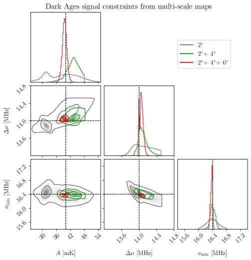
Our second finding is that larger beams are better at foreground separation than finer ones, both for chromatic and achromatic cases. One might naively expect that smaller beams will give more independent samples, providing a more complete set of ”training” and that by mixing fewer independent regions would at the same time be simpler to explain. In fact, we find some bias (at 2 sigma level) for the $6^{\circ}$ achromatic case indicating that perhaps the training set is incomplete at this resolution. We caution that with more complex foregrounds, a finer resolution data might still perform better.

Our third finding is that multi-scale fits help a lot. In achromatic case, combining 3 scale improves the uncertaint on amplitude parameter by a factor fo $\sim 4$ over the best single scale, while for the chromatic case, the improvement is even larger $\sim 10$ times. We show this in the Figure 4. Multiple scale bring more information and create a more constraining uni-modal posterior surface.

We note that the $2^{\circ}+4^{\circ}$ noiseless case seems to have much larger error bars, and does so consistently across SINF random seed choice. Compared with, for example, $2^{\circ}+4^{\circ}$ with $1\%$ gain fluctuations (see Section 5.3.1) which seems to follow an expected pattern in errorbar-size, this seems to be an isolated oddity. Therefore, we believe this effect is due to some anomalous pathological detail and would most likely go away with an investigation in stable regularization for the normalizing flow. We leave this investigation for future work.

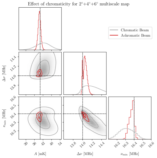
Our final finding is that beam chromaticity hurts, because it makes that measured foregrounds considerably more complex, as discussed in for example (Hibbard et al., 2020). For individual single scale measurements, the errors increase by around a factor of 10. Multi-scale fits are capable of remedying this somewhat so for $2^{\circ}+4^{\circ}+6^{\circ}$ beams, the results are only a factor of $\sim 3$ worse. We illustrate this in Figure 5. Having clean, achromatic beams helps!

5.2 Effects of the noise

We proceed by adding measurement noise. In our current approach we simply add white homogeneous noise across the full data map and leave the method unchanged.

We label the level of noise by its level in 1 MHz bins for the monopole measurement over the cut sky. In other words, 1 mK noise implies that in the absence of foreground, we would measure the monopole with 1 mK error in each MHz bin. Of course, the level of noise in each direction is then larger by square root of the number of pixels. When considering the multi-scale fits, we first add noise to the fine-scale map and then coarse this map to obtain maps coarser maps. We are in effect simulating a 2 degree experiment map on which the multi-scale technique has been applied.

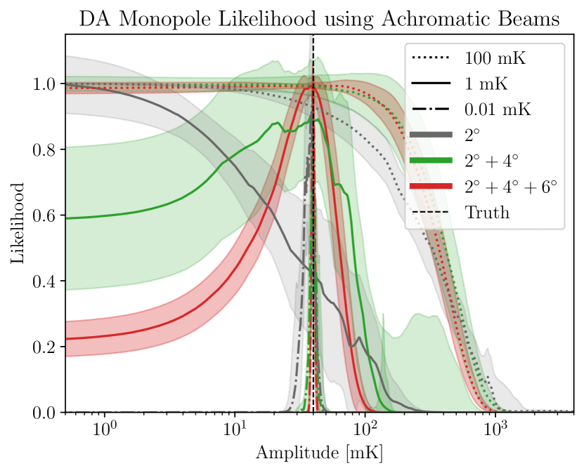
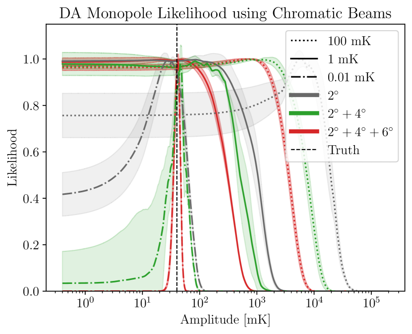
We see that the noise degrades our ability to measure the signal astonishingly fast. At noise levels exceeding 1 mK, we loose ability to detect the signal. The main reason for this is that we are learning about the properties of our foregrounds from individual directions in the sky. Since we need to understand the foreground model and the expected monopole precision, we need the relevant noise-level at the per-resolution element and not in aggregate. To detect 50mK signal we thus need approximately $\sqrt{N_{\rm pix}}~{}100$ better signal that a naive radiometer equation would imply.

The results are further scrutinized in Figures 6 and 7. We find that averaged over multiple likelihoods, the correct amplitude of the dark ages signal is measured and that results depend on the noise realization as expected.

Figure 4: Constraints on the amplitude, width and center of the DA signal from multiscale maps. Shown here is the case for 0.01mK noise level. While even a single scale is capable of isolating the allowed region around the the right answer, we find that the likelihood is multi-modal. Adding additional scales both improve the signal to noise while “pruning” wrong solutions and making the posterior surface unimodal and closer to a Gaussian.

Figure 5: Effect of chromaticity of the beams on constraints on the amplitude, width and center of the DA signal from multiscale maps. Shown here is the case for 0.1mK noise level. Note that the method itself is able to work out that the foregrounds demonstrate less intrinsic variation in the achromatic case than the chromatic case in an unsupervised way, leading to stronger constraints.

Figure 6: Likelihoods for the amplitude of the Dark Ages signal at different noise levels, and for different multi-scale combined maps using achromatic beams. The solid lines represent the median likelihoods and the shaded regions correspond to the variation across 10 different noise realizations. The dashed vertical line at $40$mK is the given fiducial amplitude for the Dark Ages.

Figure 7: Same as Figure 6 but for chromatic beams.

5.3 Instrumental effects

We study two instrumental effects: gain fluctuations and overall bandpass structure.

5.3.1 Gain fluctuations

Gain fluctuations are inevitable in any radiometer. In standard smoothness based foreground separation approaches they are completely harmless, because they do not change the smoothness of either foregrounds or the signal of interest. In our case, however, they are potentially fatal, because they leak the signal of interest into signal fluctuations. Concretely, for a sky direction for which the frequency gain $g$ has drifted from unity, we have

$$\Delta T_{\rm fg}\rightarrow g\Delta T_{\rm fg}+(1-g)\bar{T}_{\rm fg}+(1-g)T_{s}.$$ (8)

While the first two terms are likely harmless, the last term will leak the shape of the signal into fluctuations. The foreground model will then recognize this shape as foreground, at the level of $(1-g)$. We therefore expect the ability to measure the signal amplitude to be limited to the RMS of gain fluctuations.

Of course, gain fluctuations do average over time and number of observations. If the same patch of the sky is observed $N$ times, the rms of gain fluctuations will decrease by $1/\sqrt{N}$. In order to simulate the most realistic $1/f$ type gain fluctuation effects we generate a Gaussian random field smoothed on $\ell=30$ scale in harmonic space and then generate gain fluctuations consistent with such level. Results are also present in the Table 1. We see that gain fluctuations do hamper our ability to extract the signal, they do so modestly. In particular, the effect of multiscale maps is further “average” out them.

5.3.2 Overall throughput calibration

Smoothness-based separation relies on the assumption that foregrounds vary more smoothly in frequency space than the 21cm signal. Systematic effects that change the overall throughput can therefore have catastrophic impact on result. A canonical example is cable reflection, which imprints a sinusoidal structure in the overall shape of the throughput. If sufficiently sharp, such feature can be mistaken for a signal.

In our case, any function $g(\nu)$ that is purely multiplicative in frequency only changes the eigenvectors of the problem, which also get multiplied by $g(\nu)$. Everything else, including the decomposition into the PCA basis and consequently the likelihood calculation remains exactly the same. So ultimately, the only error we are making is using the wrong basis vectors when calculating the likelihood of a given theretical model.

To calculate the impact of this systematic we consider a “cable reflection” type effect with

$$g(\nu)\rightarrow\left(1+A_{c}\cos(\omega_{c}\nu)\right),$$ (9)

where we fix $\omega_{c}$ to have three full cycles across the 50MHz band and vary $A_{c}$.

Results are also shown in Table 1. Note that in this case we do not expect a change in accuracy, but we migh expect a bias in the results. While we see that results do change, they are surprisingly stable.

5.4 Detecting CMB

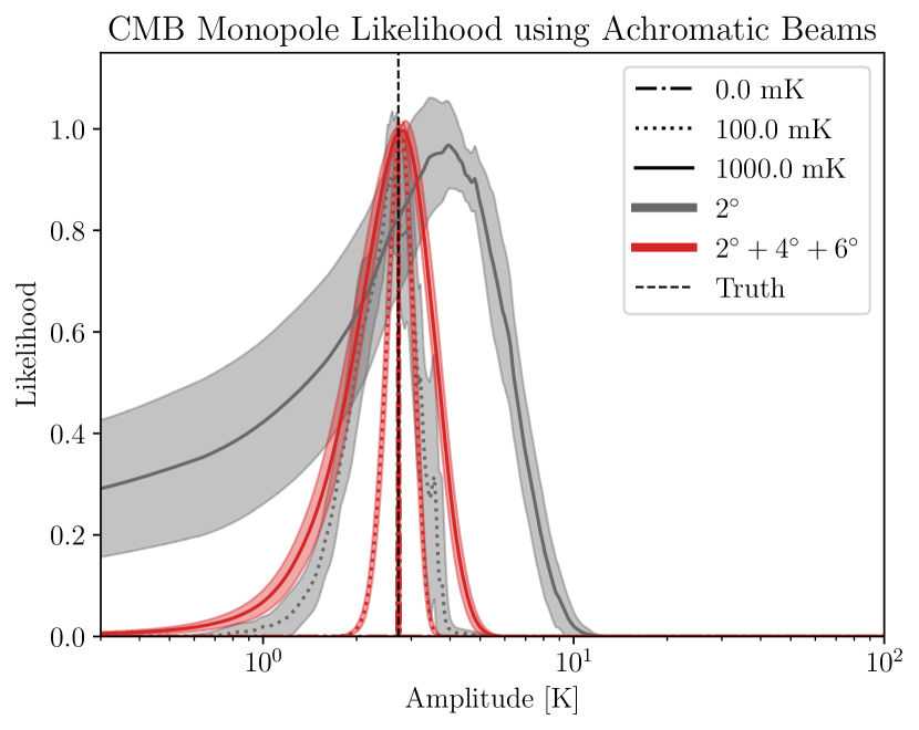
In Table 2 we present the results for the CMB monopole signal for a $2^{\circ}$ instrument with and without chromaticity, along with the improvements due to a multiscale $2^{\circ}+4^{\circ}+6^{\circ}$ fit. We see a surprisingly strong detection of the signal. While CMB is very smooth, it at the same time has a very different spectral shape, being a power-law with spectral index zero compared to foregrounds which are a power law with a spectral index $\approx-2.5$. CMB signal is recovered very well at moderate noise levels as one would expect. The CMB signal being two orders of magnitude large in amplitude compared to Dark Ages signal should be the prime target for the first generation of Dark Ages experiments.

In Figure 8 we show some of the typical likelihood surfaces associated with the CMB temperature.

Figure 8: CMB amplitude constraints for an achromatic $2^{\circ}$ beam at various noise levels. Solid lines represent the median likelihoods and colored regions represent the error bounds derived from a set of 10 different noise realizations.

Noise [mK]	$A$ [K]	$95\%$ C.L.
Truth	$2.725$
$2^{\circ}$ Beam
Achromatic
0mK	$2.747^{+0.011}_{-0.011}$	$<2.761$
100mK	$2.487^{+0.472}_{-0.573}$	$<3.321$
1000mK	$1.855^{+2.431}_{-1.266}$	$<6.002$
Chromatic
0mK	$2.631^{+1.038}_{-1.112}$	$<4.329$
100mK	$2.743^{+5.987}_{-2.120}$	$<13.379$
1000mK	$11.855^{+22.239}_{-10.651}$	$<46.752$
$2^{\circ}+4^{\circ}+6^{\circ}$ Beam
Achromatic
0mK	$2.747^{+0.011}_{-0.011}$	$<2.761$
100mK	$2.816^{+0.258}_{-0.262}$	$<3.242$
1000mK	$2.622^{+0.803}_{-0.831}$	$<3.939$
Chromatic
0mK	$2.742^{+0.040}_{-0.038}$	$<2.807$
100mK	$2.305^{+1.900}_{-1.525}$	$<5.395$
1000mK	$1.661^{+3.246}_{-1.160}$	$<7.728$

Table 2: Results for CMB monopole amplitude constraints and $95\%$ confidence limits (C.L.) for a $2^{\circ}$ beam

6 Discussion & Conclusions

We have presented a new method for extracting presence of monopole signal in radio experiments. The method can successfully extract any monopole that is sufficiently statistically different from the foreground signal assuming the fluctuations in the foreground are representative of their mean signal.

We have argued that the traditional smoothness based separation is very difficult to put in practice in the presence of the strong foregrounds and antenna chromaticities, since any residual effects would have to be controlled at a one-part in a million, many orders of magnitude beyond the current state of the art. Instead we have presented a method where we can build a model for foreground fluctuations in an unsupervised way and apply the model to filter out the foreground monopole. The assumption that this is a valid procedure is based on the physical intuition that the foreground generating process is local in space.

We have considered extracting information from multiple scales. We find that fitting multiple scales at once can bring significant benefits in terms of signal-to-noise.

We have demonstrated that the method works for semi-realistic sky models and instrument, but requires high signal-to-noise. In a traditional, smoothness-based separation, the requirement is that the noise level is small compared to the signal over the entire sky. In this case, we need to learn about possible spectra shapes of foregrounds at the level of the signal of interest, and therefore we require noise level to be small compared to signal in individual resolution elements. Nevertheless, a sufficiently aggressive instrument would reach the required sensitivities. Assuming $10^{5}$ K foregrounds, it would take $10^{4}$ detectors 10 lunar nights to reach radiometric sensitivity of $0.3$ mK – while clearly an ambitious experiment it is not deliriously insane to consider it possible in the next few decades. We stress that these results are obtained without any specific optimization. By focusing on the quiet parts of the sky with optimized beam sizes, etc one might be able to do considerably better.

We found that antenna design matters and that achromatic experiments do significantly better, since there is less mixing of foreground shapes. But our method is automatic and does not impose any hard requirements: the less chromatic your instrument response, the better results you will obtain in a self-consistent and self-calibrating manner. Our approach also relaxes requirements on the system throughput shape and presence of overal gain fluctuations. Perturbations at 1% level are sufficient to extract the signal.

These considerations have deep implications for the design of the experiments to measure the 21 cm monopole signal. Instead of having a low-resolution instrument with exquisitely calibrated and designed beam, a better strategy is a higher-resolution instrument with small gain fluctuations and sub-percent level understanding of ground coupling. Such an instrument would target a smaller, quieter patch of the sky to the extreme depths required to measure the signal.

Somewhat surprisingly we have found that coarser resolution is easier to model, at least in the simulated data. Whether this also holds true for real sky remains to be seen. The foreground modelling over at high resolution is likely easier, since the emission is more localized, and we have more samples of the foreground fluctuations that enable us to build a more robust foreground model.

We have also found that our method is surprisingly good at extracting the CMB monopole signal. Measuring the CMB signal deep in the Rayleigh-Jeans regime would be an important milestone on the way to detecting more interesting signals. Assuming alternative scenarios are excluded, this could also act as a calibration signal, tying the overall temperature scale to very precisely known CMB temperature. One might worry that the CMB signal would be perfectly degenerate with the amplifier noise, but in practice this should not be the case. This is because the presence of the ground (or the lunar regolith) as well as the frequency dependent preamplifier coupling will make the amplifier noise contribution non-white once the signals are express in the units of sky monopole.

There are several avenues for improving and extending our method. The first is to optimize the linear combinations of the raw data that are used for analysis. For example, we have shown that achromatic beams perform better. With a sufficiently high native resolution, it should be possible to generate synthetic achromatic beams that might perform better than raw data. We have found that the particular combination of $2^{\circ}$, $4^{\circ}$ and $6^{\circ}$ degrees beams performs considerably better than individual resolutions without any attempts to fine-tune the results. In practice, these design and analysis choices can likely be improved, but they are also highly likely to be strongly dependent on the details and complexity fo the assumed sky model. Further optimization lies also in the frequency resolution and sky coverage.

Finally, this method can be applied on existing data from cosmic dawn measurements in order to constrain the various parameters like the depth, width and center of the absorption signal.

Appendix A Numerical Care with PCA decomposition

Typically, PCA decomposition of a data vector $\mathbf{X}\in\mathbf{R}^{m\times n}$ can be done in two equivalent ways viz. eigen-decomposition of the covariance matrix of the data $\mathrm{cov}(\mathbf{X})=\mathbf{U}S\mathbf{U}^{T}$ where $\mathrm{cov}(\mathbf{X})=\frac{1}{\sqrt{n-1}}\mathbf{X}^{T}\mathbf{X}$, or singular value decomposition $\mathbf{U}S\mathbf{V}^{T}=\mathbf{X}$ of the data directly. It is straightforward to show that these methods are identical, upto signs, for calculating $\mathbf{U}$ and their eigenvalues $S$.

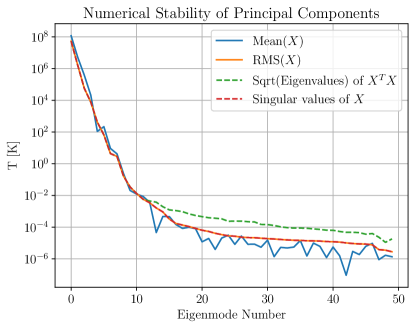
A typical float64 number has $\sim 15$ digits of precision. If the relative difference between the smallest and largest numbers in your data $X$ exceed $10^{8}$ in arbitrary units, then squaring the data vector is numerically unstable since the float64 data type is unable to offer the required precision for the smallest and the largest entries simultaneously. This is a known numerical issue involving the calculation of the covariance matrix of a data vector that contains elements $O(1)$ along with elements $\epsilon\sim 10^{-8}\ll O(1)$. The computation $\mathbf{X}^{T}\mathbf{X}$ can lead to a loss of precision and give numerically unstable eigenvectors/values.

This can be seen in Figure 9 where the PCA eigenvalues (rather their square roots) should in principle correspond with the data RMS seem to deviate starting at the precision limit. This is an indication that the underlying eigenvectors are numerically inaccurate. Compared with the eigenvalues from SVD, the data RMS agrees well with the singular values as expected.

Performing singular value decomposition is much more stable numerically, since it involves computation on the data $\mathbf{X}$ directly. However, since the products of SVD also involve the very large $\mathbf{V}$ matrix of shape $(\texttt{npix}\times\texttt{npix})$ the memory requirements for this step can be substantial.

Figure 9: Numerical stability of the method used for finding the principal components of a data vector $X$. Note the orange line, representing the true RMS values of the data, agrees well with the singular values (dashed red) obtained directly from $X$. However, compared to the eigenvalues (dashed green) obtained from the covariance matrix $X^{T}X$, we can see that there is a disagreement as the required relative precision in $X$ approaches $\sim 10^{-10}$, corresponding to a relative precision of $\sim 10^{-20}$ in the $X^{T}X$ computation which is not possible with the float64 datatypes.

Appendix B Intrinsic variation of SINF

For each run, SINF converges slightly differently due to intrinsic random nature of slicing the base distribution in the process of mapping to the target distribution. For a fixed noise realization, the spread in likelihood is smaller than, if not comparable to, the variation due to different noise realizations. Shown in Figure 10 for $\sigma=2^{\circ}$ chromatic noiseless beams and for the achromatic case with $100$ mK noise. This exercise also guarantees that the SINF algorithm is sufficiently confident of its density estimation and converges stably.

Figure 10: Variations within fixed noise realizations for a chromatic beam with no noise (left) and an achromatic beam at 100mK noise (right)

References

- Pritchard and Loeb (2012) J. R. Pritchard and A. Loeb, Rep. Prog. Phys. 75, 086901 (2012), arXiv:1109.6012 [astro-ph].
- Furlanetto (2019) S. R. Furlanetto, “The Fundamentals of the 21-cm Line,” (2019), arXiv:1909.13740 [astro-ph].
- Bowman et al. (2018) J. D. Bowman, A. E. E. Rogers, R. A. Monsalve, T. J. Mozdzen, and N. Mahesh, “An absorption profile centred at 78 megahertz in the sky-averaged spectrum,” (2018), arXiv:1810.05912 [astro-ph].
- Singh et al. (2021) S. Singh, J. N. T., R. Subrahmanyan, N. U. Shankar, B. S. Girish, A. Raghunathan, R. Somashekar, K. S. Srivani, and M. S. Rao, “On the detection of a cosmic dawn signal in the radio background,” (2021), arXiv:2112.06778 [astro-ph].
- Hills et al. (2018) R. Hills, G. Kulkarni, P. D. Meerburg, and E. Puchwein, (2018), 10.1038/s41586-018-0796-5, arXiv:1805.01421 .
- Bradley et al. (2019) R. F. Bradley, K. Tauscher, D. Rapetti, and J. O. Burns, ApJ 874, 153 (2019), arXiv:1810.09015 [astro-ph].
- Pospelov et al. (2018) M. Pospelov, J. Pradler, J. T. Ruderman, and A. Urbano, Phys. Rev. Lett. 121, 031103 (2018), arXiv:1803.07048 [hep-ph] .
- Caputo et al. (2023) A. Caputo, H. Liu, S. Mishra-Sharma, M. Pospelov, and J. T. Ruderman, Phys. Rev. D 107, 123033 (2023), arXiv:2206.07713 [hep-ph] .
- Acharya and Chluba (2023) S. K. Acharya and J. Chluba, MNRAS 521, 3939 (2023), arXiv:2209.09063 [astro-ph.CO] .
- Dowell and Taylor (2018) J. Dowell and G. B. Taylor, ApJ 858, L9 (2018), arXiv:1804.08581 [astro-ph.CO] .
- Fixsen et al. (2011) D. J. Fixsen, A. Kogut, S. Levin, M. Limon, P. Lubin, P. Mirel, M. Seiffert, J. Singal, E. Wollack, T. Villela, and C. A. Wuensche, ApJ 734, 5 (2011), arXiv:0901.0555 [astro-ph.CO] .
- Sathyanarayana Rao et al. (2015) M. Sathyanarayana Rao, R. Subrahmanyan, N. Udaya Shankar, and J. Chluba, ApJ 810, 3 (2015), arXiv:1501.07191 [astro-ph.IM] .
- Bevins et al. (2020) H. T. J. Bevins, W. J. Handley, A. Fialkov, E. de Lera Acedo, L. J. Greenhill, and D. C. Price, (2020), 10.1093/mnras/stab152, arXiv:2007.14970 .
- Tauscher et al. (2018) K. Tauscher, D. Rapetti, J. O. Burns, and E. R. Switzer, ApJ 853, 187 (2018), arXiv:1711.03173 [astro-ph].
- Bassett et al. (2021) N. Bassett, D. Rapetti, K. Tauscher, J. Burns, and J. Hibbard, ApJ 908, 189 (2021), arXiv:2011.01242 [astro-ph].
- Cong et al. (2021) Y. Cong, B. Yue, Y. Xu, Q. Huang, S. Zuo, and X. Chen, ApJ 914, 128 (2021), arXiv:2104.03170 [astro-ph].
- Górski et al. (2005) K. M. Górski, E. Hivon, A. J. Banday, B. D. Wandelt, F. K. Hansen, M. Reinecke, and M. Bartelmann, The Astrophysical Journal 622, 759 (2005), aDS Bibcode: 2005ApJ…622..759G.
- Dai and Seljak (2021) B. Dai and U. Seljak, “Sliced Iterative Normalizing Flows,” (2021), arXiv:2007.00674 [cs, stat].
- Mirocha (2014) J. Mirocha, Monthly Notices of the Royal Astronomical Society 443, 1211 (2014), arXiv:1406.4120 [astro-ph].
- Hibbard et al. (2020) J. J. Hibbard, K. Tauscher, D. Rapetti, and J. O. Burns, ApJ 905, 113 (2020), arXiv:2011.00549 [astro-ph].