On Time Domain Conformer Models for Monaural Speech Separation in Noisy Reverberant Acoustic Environments

Abstract

Speech separation remains an important topic for multi-speaker technology researchers. conformer have performed well for many speech processing tasks but have been under-researched for speech separation. Most recent state-of-the-art (SOTA) separation models have been TasNets. A number of successful models have made use of dual-path (DP) networks which sequentially process local and global information. TD-Conformer are an analogue of the DP approach in that they also process local and global context sequentially but have a different time complexity function. It is shown that for realistic shorter signal lengths, conformers are more efficient when controlling for feature dimension. Subsampling layers are proposed to further improve computational efficiency. The best time domain conformer (TD-Conformer) achieves $14.6$ dB and $21.2$ dB SISDR improvement on the WHAMR and WSJ0-2Mix benchmarks, respectively.

Index Terms: speech separation, conformer, speech enhancement, time domain, single channel

1 Introduction

Deep neural network models have led to significant improvements in monaural speech separation technology in recent years [1, 2, 3, 4]. While impressive results have been attained on clean speech mixtures, noisy and reverberant mixtures still remain a challenging and active area of research [5, 6, 7, 8].

Transformer TasNet models have demonstrated SOTA performance on numerous benchmarks in recent years [9, 10, 11, 4] due to their ability to process the global context of sequences. Many of these models used DP networks [12, 9, 10]. The conformer is a similar concept to DP and quasi-DP approaches [12, 10, 4] but uses a single convolutional layer to process the local context instead of a more computationally complex recurrent neural network (RNN) or transformer layer. A benefit of this is reduced computational complexity as convolutional operations are more parallelizable along all dimensions and have linear time-complexity (TC) [8]. A short-time Fourier transform (STFT)-based conformer model has been proposed for continuous speech separation in [13] which shows reasonable performance on the LibriCSS dataset but does not compare to popular time-domain techniques on other popular benchmarks as it is shown in Section 5.3, most likely due to its lower temporal resolution as [14] similarly demonstrated. A time-domain conformer and a temporal convolutional network (TCN)-augmented conformer model were proposed for speech extraction in [15]. The TCN model performs best but has a much wider local context window, or receptive field (RF), than the pure conformer model. Questions remain about whether the full TCN approach is necessary if a convolutional module in a conformer were to have a sufficiently wide kernel size [15, 4] and comparable model size, as this was not analysed in [15].

In this work, a single channel TD-Conformer model is evaluated across different model sizes and computational expenditures from both theoretical and experimental perspectives. While TasNets and conformer models are well studied, the combination of the two for separation tasks with a corresponding optimisation and performance analysis is as yet missing from the speech separation literature. Furthermore, this work demonstrates why it is an oversight in the area of speech separation research to not explore this particular combination in greater depth given the proposed model configuration in this paper is able to achieve close to SOTA results with useful trade-offs in computational expenditure for the separation of shorter speech utterances. It is shown in this work that, in the local-layer global-layer paradigm often used in speech separation deep neural network (DNN) models [12, 9, 10], convolution augmented transformer (conformer) layers can be a more computationally suitable option in terms of efficiency. In this work, a subsampling method is introduced which further reduces the computational TC of the dot product attention in the transformer layers, similar to the SE-Conformer model [16]. A number of evaluations are performed to assess the optimal RF [17] of the convolutional component in the conformer, the impact of subsampling on performance and computational complexity, and the benefits of the time domain approach over the STFT model proposed in [13]. Results are compared to a number of other SOTA models in terms of performance, model size, and computational complexity across multiple benchmarks and acoustic conditions.

The remaining paper proceeds as follows. Section 2 introduces the signal model and Section 3 the proposed TD-Conformer model. Datasets and training configurations are explained in Section 4 and results are presented in Section 5. Section 6 gives final conclusions.

2 Signal Model

A noisy discrete-time reverberant mixture signal $x[i]$ of $C$ speakers $s_{c}[i]$ with additive noise $n[i]$ at the microphone is defined as

$$x[i]=\sum_{c=1}^{C}s_{c}[i]\ast h_{c}[i]+n[i],$$ (1)

where the operator $\ast$ denotes the convolution and $h_{c}[i]$ is the room impulse response (RIR) corresponding to speaker $c\in\{1,\ldots,C\}$. In this work the aim is to find an estimate for each of the $C$ speech signals, denoted by $\hat{s}_{c}[i]$.

3 TD-Conformer Separation Networks

The proposed TD-Conformer, described in the following, is a TasNet composed of three main components: a feature encoder, a mask estimation network and a decoder as depicted in Figure 1. The encoder is a learnable filterbank [2, 18] and the decoder performs the inverse function to convert encoded features back into the time domain. The mask estimation network calculates $C$ masks $\mathbf{m}_{\ell,c}$ for each time frame $\ell$ to obtain estimates $\mathbf{\hat{s}}_{\ell,c}$ of the clean input speech signals $\mathbf{s}_{\ell,c}$. Boldface letters indicate vectors capturing respective frames of samples of the quantities in Section 2.

Fig. 1: TD-Conformer TasNet model diagram, exemplary for $C=2$ speakers for each frame index $\ell$. Operator $\odot$ denotes the Hadamard product and $\mathbf{w}_{\ell}$ the vector of encoded features for frame $\ell$.

3.1 Encoder

Similar to [10, 19], the mixture signal $x[i]$ in (1) is segmented into $L_{\mathbf{x}}$ overlapping blocks $\mathbf{x}_{\ell}$ of size $L_{\mathrm{BL}}$ which are encoded into $\mathbf{w}_{\ell}\in\mathbb{R}^{1\times N}$ using a 1D convolutional layer with weights $\mathbf{B}\in\mathbb{R}^{L_{\mathrm{BL}}\times N}$ for $N$ output channels, followed by a ReLU activation function $\mathcal{H}_{\mathrm{enc}}:\mathbb{R}^{1\times N}\rightarrow\mathbb{R}^{1\times N}$ producing encoded features

$$\mathbf{w}_{\ell}=\mathcal{H}_{\mathrm{enc}}\left(\mathbf{x}_{\ell}\mathbf{B}\right)\in\mathbb{R}^{L_{\mathrm{x}}\times N}.$$ (2)

3.2 Conformer Mask Estimation Network

The mask estimation network is based on the conformer architectures proposed in [20, 16]. A diagram of the conformer mask estimation network is shown in Figure 2.

Fig. 2: Proposed TD-Conformer mask estimation network structure with subsampling and supersampling layers to reduce and increase the temporal resolution, and also enabling a reduction of the time-complexity (TC) in the conformer layers.

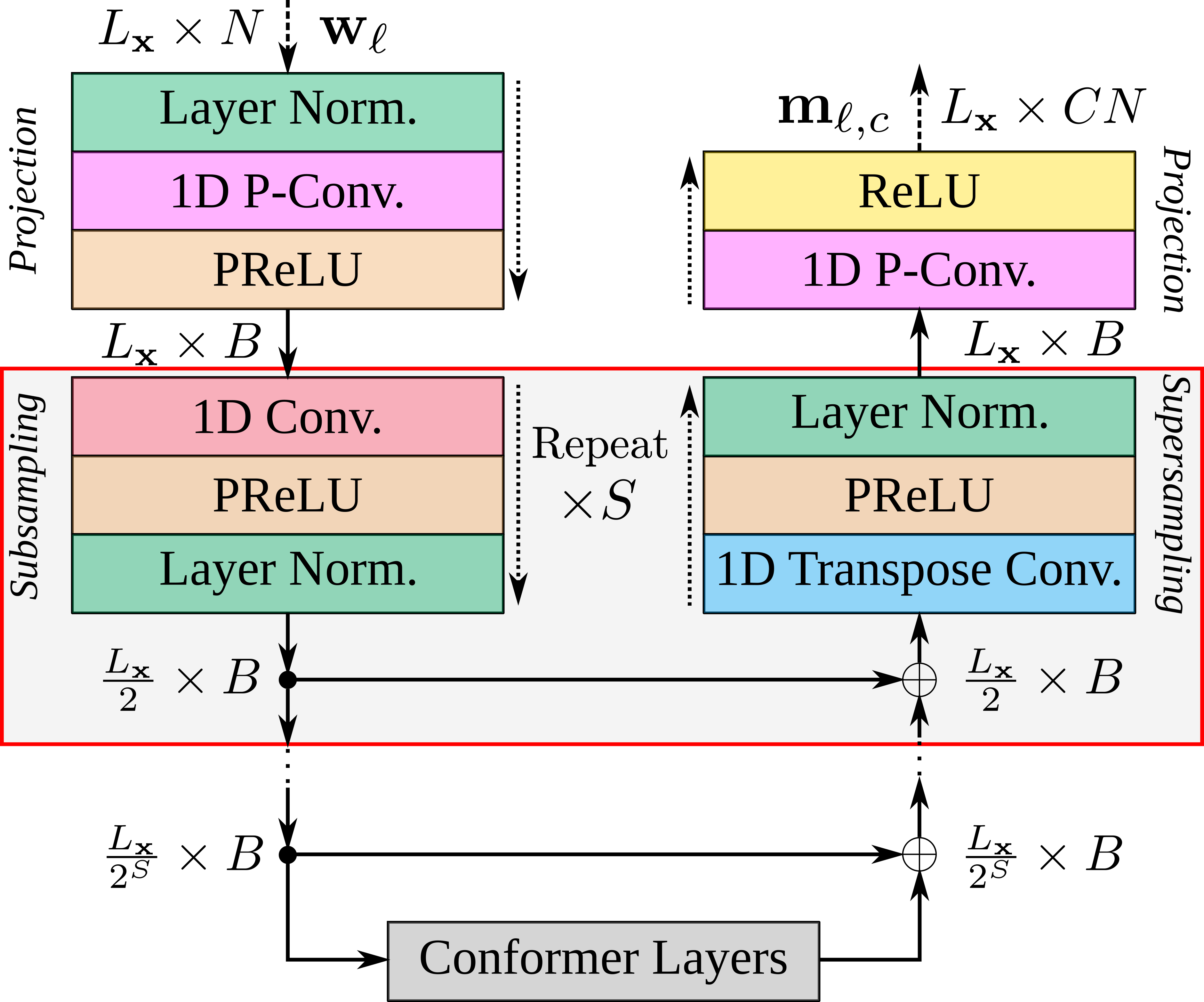
The input sequence of features $\mathbf{w}_{\ell}$ is normalized using layer normalization [21] before being projected from dimension size $N$ to $B$ using a pointwise convolution (P-Conv) layer followed by a parametric (PReLU) activation. This results in a sequence of features of shape $L_{\mathbf{x}}\times B$. This sequence is then fed through $S$ subsampling layers each of which is a 1D convolutional layer of a fixed kernel size of $4$ and stride of $2$ thus reducing the temporal dimension by a factor of $2$ giving a sequence of shape $\frac{L_{\mathbf{x}}}{2^{S}}\times B$. Each subsampling layer has a skip connection to a respective supersampling block composed of a 1D transposed convolutional layer, PReLU and layer normalization. This structure increases the temporal dimension by a factor of $2$ to restore the sequence length to $L_{\mathbf{x}}$. In between the subsampling and supersampling blocks are a series of $R$ conformer layers.

The conformer layers are shown in detail in Figure 3 and are composed of a feed-forward module, a convolution module, a multihead self-attention (MHSA) module and another feed-forward module. The convolution module comes before the MHSA module contrasting the original conformer [20] which has MHSA first. This is so the model processes the local context first similar to the DP models proposed in [12, 10].

Fig. 3: Diagram of a single Conformer layer composed of feed-forward, convolution and MHSA modules. Note the first feed-forward module is identical to the final module but its details are omitted for brevity.

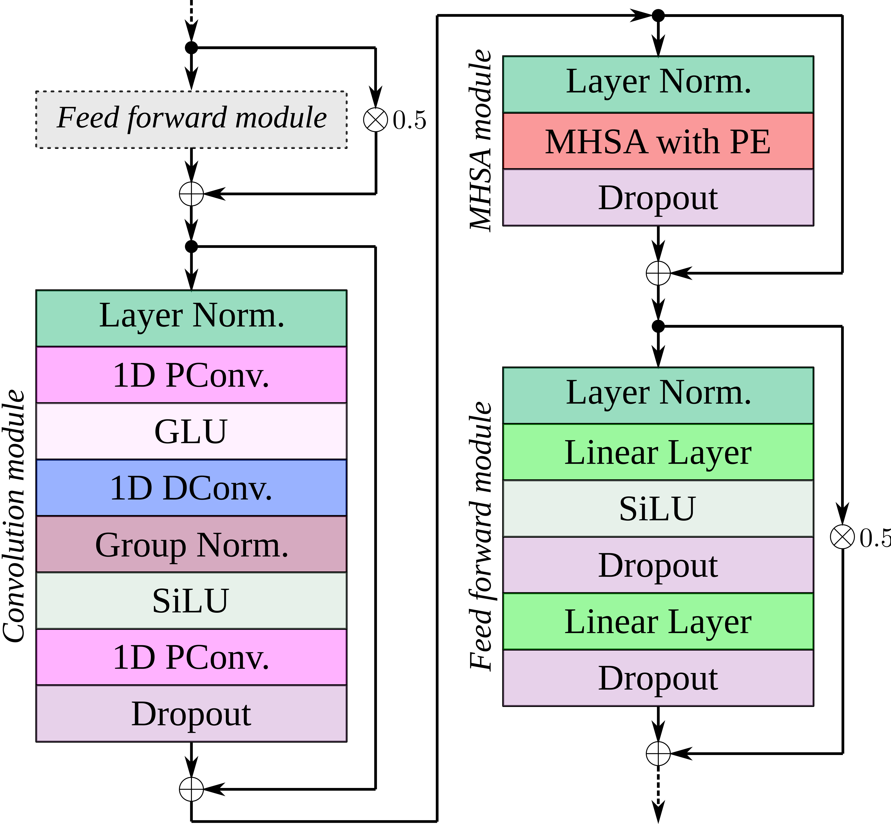
The two feed-forward modules are composed of layer normalization, a linear layer with sigmoid linear unit (SiLU) activation [22], dropout [23] and then another linear layer followed by another dropout. Each feed-forward module has a weighted residual connection from input to output. The convolution module is composed of layer normalization, a P-Conv with gated linear unit (GLU) activation, a depthwise convolution (D-Conv) with kernel size $P$, group normalization [24], a SiLU activation and lastly a P-Conv layer followed by dropout. For the group normalization, the number of groups is equal to the number of input channels. A residual connection goes from the input to the output of the module. The MHSA module is composed of layer normalization and MHSA with relative positional encoding (PE) [25] followed by dropout. The MHSA module has a residual connection around the entire module.

3.3 Conformers vs. Dual-Path Transformers

The conformer layers are proposed in analogy to the DP transformer layers in the widely researched SepFormer model [10, 14]. Note that other DP transformer layers have been proposed, such as in [9], but we disregard these here as they are more computationally expensive and less performant than SepFormer [10, 26]. In this section, the respective TC functions of the conformer layer and the DP transformer layer are modelled to demonstrate that under certain (often more realistic) signal lengths and feature dimensions, conformers are less computationally complex than DP transformers. The intra-transformer is compared to the convolutional module of the conformer as a local context layer and the inter-transformer is compared to MHSA modules of the conformer as a global context layer. The TC for a conformer layer is defined as

$$\mathcal{T}_{\mathrm{Conf}}=\frac{L_{\mathbf{x}}}{2^{S}}\left(PB+B^{2}\right)+\frac{L_{\mathbf{x}}^{2}}{2^{2S}}B+B^{2}\frac{L_{\mathbf{x}}}{2^{S}}.$$ (3)

The TC for a dual-path transformer layer in the style of SepFormer [10] is defined as

$$\mathcal{T}_{\mathrm{DPT}}=\left(\frac{L_{\mathbf{x}}}{2P^{\prime}}+\frac{P^{\prime}}{2}\right)\left(P^{\prime 2}B+B^{2}P^{\prime}\right)+\frac{L_{\mathbf{x}}}{4P^{\prime 2}}B+B^{2}\frac{L_{\mathbf{x}}}{2P^{\prime}},$$ (4)

where $P^{\prime}$ represents the chunk size [10]. The time-complexities for DP transformer and conformer layers with a feature sequence from an 8kHz piece of audio encoded with block length $L_{\mathrm{BL}}=16$ are shown in Figure 4 for different feature dimensions $B$.

Fig. 4: Comparison of TCs measured in GFLOPS for a conformer layer and a DP Transformer layer for different feature dimensions $B\in\{128,256,512\}$ over relative signal length in seconds. Note that $S=0$ for the Conformer layer here and $P=P^{\prime}=250$ is used as it is equal to the best performing configuration of the DP model in [10].

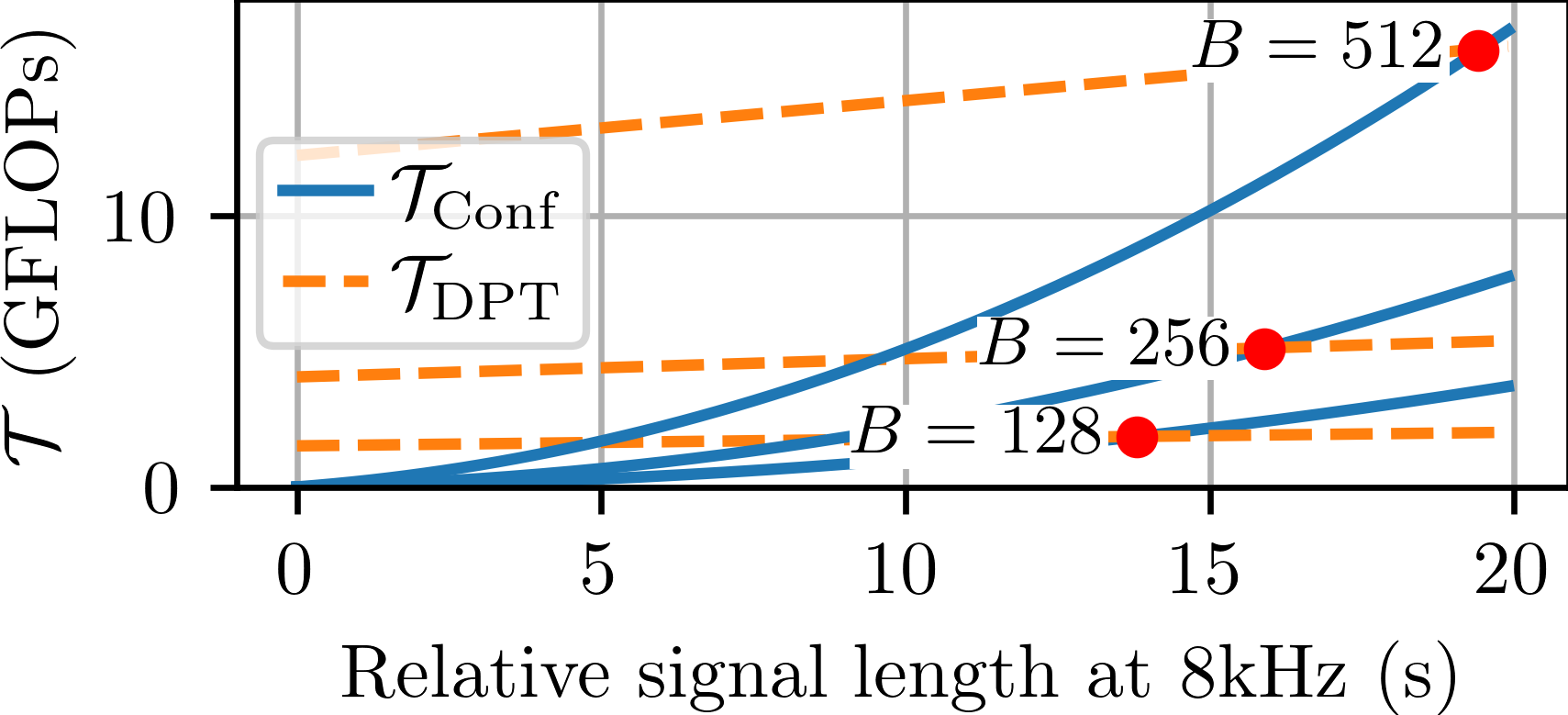
The average and maximum signal lengths in the WHAMR tt evaluation set used later in Section 5, are $5.79$s and $13.87$s, respectively [27]. Hence, in evaluations on this dataset, the conformer layer is the less computationally complex option overall. For larger $B$ values the conformer more likely has lower TC than the DP transformer. Another benefit of the conformer is that, assuming a small number of subsampling layers, it has a much higher temporal resolution than the DP approach when processing the global context.

Fig. 5: Comparison of conformer TC function over relative signal length for varying subsampling layers $S\in\{0,1,2,3\}$.

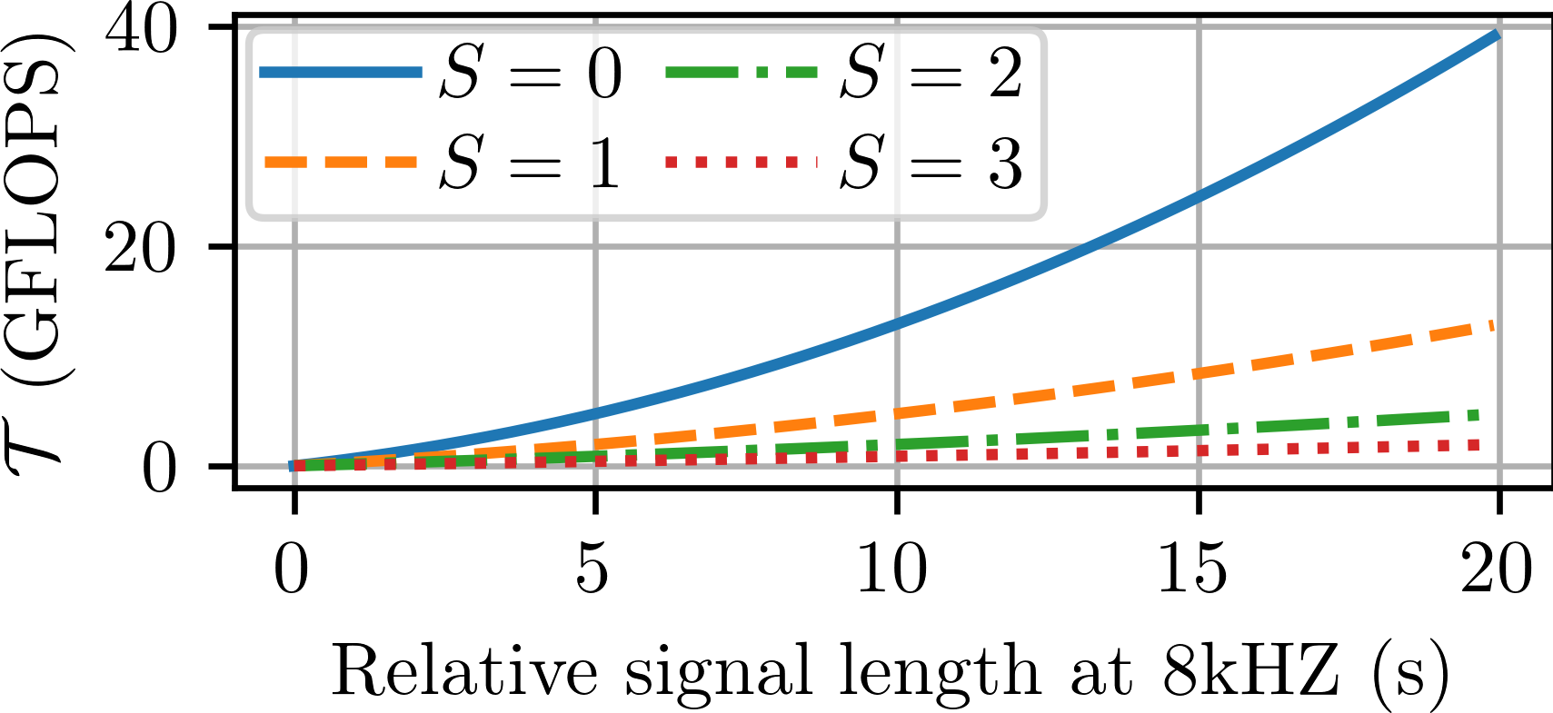
Figure 5 demonstrates that every additional subsampling layer can significantly reduce the TC of the conformer layer. The impact of increasing the subsampling on overall performance is explored in more depth later in Section 5.2. Note that the DP transformer topology also has its own implicit subsampling strategy akin to a strided view of the output tensor from the local transformer layer which reduces the computational complexity but also the temporal resolution significantly [4, 10].

3.4 Objective function

An scale-invariant signal-to-distortion ratio (SISDR) objective function [28, 2] with an utterance-level permutation invariant training (uPIT) wrapper [1] is used to train all of the models. The SISDR loss function is defined as

$$\mathcal{L}(\hat{\boldsymbol{\mathrm{s}}},\boldsymbol{\mathrm{s}}) :=\frac{1}{C}\sum_{c=1}^{C}-10\log_{10}\frac{\left\|\frac{\langle\hat{\boldsymbol{\mathrm{s}}}_{c},\boldsymbol{\mathrm{s}}_{c}\rangle\boldsymbol{\mathrm{s}}_{c}}{\|\boldsymbol{\mathrm{s}}_{c}\|^{2}}\right\|^{2}}{\left\|\hat{\boldsymbol{\mathrm{s}}}_{c}-\frac{\langle\hat{\boldsymbol{\mathrm{s}}}_{c},\boldsymbol{\mathrm{s}}_{c}\rangle\boldsymbol{\mathrm{s}}_{c}}{\|\boldsymbol{\mathrm{s}}_{c}\|^{2}}\right\|^{2}}.$$ (5)

4 Experimental Setup

4.1 Data

The WHAMR and WSJ0-2Mix datasets are used for analysing the proposed TD-Conformer models [29, 7]. WSJ0-2Mix is a 2-speaker mixture corpus [29]. Speech segments from the WSJ0 corpus are mixed at speech-to-speech ratios between $0$ to $5$ dB. WHAMR is a noisy reverberant extension of WSJ0-2Mix. Ambient recorded noise is mixed with the speakers at signal-to-noise ratios between $-6$ and $3$ dB. Simulated RIRs are used to reverberate the speech mixtures with reverberation time T60 values ranging between $0.1$s and $1$s.

4.2 Network configurations

Four model configurations are proposed to vary the model size in increasing internal mask estimation feature dimension $B$ of $128$ (denoted as small (S)), $256$ ( medium (M)), $512$ ( large (L)) and $1024$ ( extra-large (XL)). The encoder has a fixed output dimension of $N=256$ and a kernel size of $L_{\mathrm{BL}}=16$ with a $50\%$ stride of $8$ samples. The number of conformer layers is fixed to $R=8$, the same as the number of DP layers in [10]. In the results sections the number of subsampling layers $S$ and conformer kernel size $P$ are modified to gain a better understanding of their impact on separation performance and computational cost. For all evaluations a dropout of $10\%$ is used.

4.3 Training configurations

All models are trained using an initial learning rate of $5\times 10^{-5}$. Learning rates are fixed for the first $90$ epochs and then halved if there is no performance improvement after $3$ epochs. Training is performed over $200$ epochs. Training examples were limited to $4$ seconds. In [27] it was shown that this signal length is in an optimal range to reduce training time without impacting overall performance for the datasets used in this paper. By limiting the training signal lengths, it enables the use of a batch size of $4$ even with the largest XL models proposed in Section 4.2. This contrasts the best performing SepFormer model where it has been shown that even with comparable TSL limits the largest batch size it was possible to use was $2$ [27] on the same GPU used in this paper, a 32GB Nvidia V100. Further to the discussion in Section 3.3, the reason for this difference is that despite both the TD-Conformer XL model and the Sepformer using an internal feature dimension of $1024$, the use of MHSA in the Sepformer for processing local information consumes a lot more memory for an utterance of $4$s in length. An open-source SpeechBrain [30] recipe is provided with this work to enable other researchers to reproduce the results in this paper.

4.4 Evaluation Metrics

The main separation evaluation metric used is SISDR improvement over the noisy mixture, denoted by $\Delta$ SISDR and measured in dB. Where relevant, computation expenditure is report using mutiply-acccumulate operations (MACs). MACs are calculated using the thop [31] toolkit on a signal of $5.79$s in length, equal to the mean signal length in the WHAMR test set. This is to be more reflective of a realistic input as the TD-Conformer models contain quadratic time complexities. Model size is measured in parameter count where relevant.

5 Results

5.1 Varying kernel sizes

In this section, the kernel size $P$ of the D-Conv layer in the conformer layer is varied for different feature dimensions $B$ to evaluate if there exists a common $P$ value. Five $P$ values are evaluated: $\{16,32,64,125,250\}$. The values $16$ and $32$ are similar to the kernel sizes in the original conformer model [20] as well as in [13, 16]. The values $64$, $125$ and $250$ were selected to give the D-Conv layer a comparable RF to the local transformer layer of popular DP models such as SepFormer [10] where the chunk size is set to $250$ for the equivalent $L_{\mathrm{BL}}=16$ model configuration. The results in Figure 6 show that for all models the performance in $\Delta$ SISDR peaks for a kernel size of $P=32$.

Fig. 6: Performance in $\Delta$ SISDR for conformer layer kernel sizes $P\in\{16,32,64,125,250\}$ and different model sizes based on $B$.

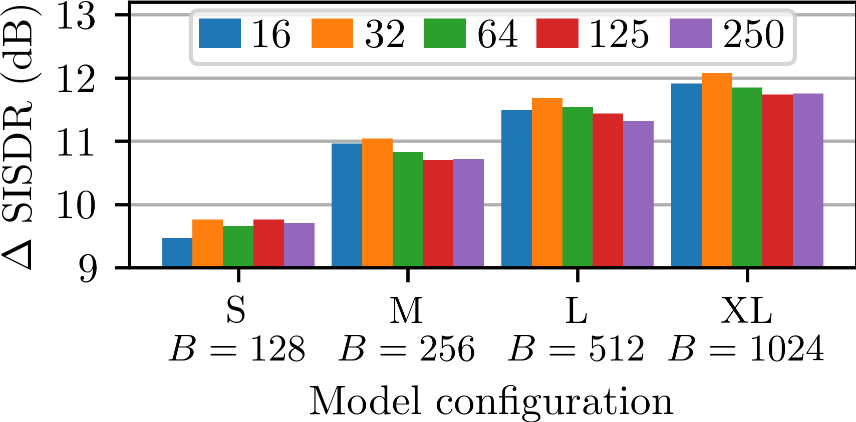
For sampling rate $\mathrm{f}_{s}$, the relative RF of each convolution module in seconds is defined as

$$\mathcal{R}_{\mathrm{conv}}(S,P,L_{\mathrm{BL}},\mathrm{f}_{s})=\frac{1}{\mathrm{f}_{s}}\left({2^{S-1}L_{\mathrm{BL}}}P+\frac{L_{\mathrm{BL}}}{2}\right)$$ (6)

which for the configuration $\{S,P,L_{\mathrm{BL}},\mathrm{f}_{s}\}=\{2,32,16,$ $8000\}$ is $0.129$s. This RF value is used later in Section 5.3 for optimising the model hyperparameters.

5.2 Varying the number of subsampling layers

Altering the number of subsampling layers changes the temporal resolution of the input encoded features to the Conformer layers in the mask estimation network. It also inversely affects the overall model size, i.e. more subsampling layers result in lower temporal resolution but slightly larger model size. In this second experiment the number of subsampling layers $S$ is varied from $0$ to $3$. Note that for $S=0$, a smaller batch size of $2$ has to be used due to the increased memory consumption of the transformer layers. A fixed kernel size of $P=32$ is used.

Fig. 7: Performance over number of subsampling layers $S$ for all conformer model sizes (S, M, L & XL) with respective computational cost in MACs exemplary for signal of length $5.79$s.

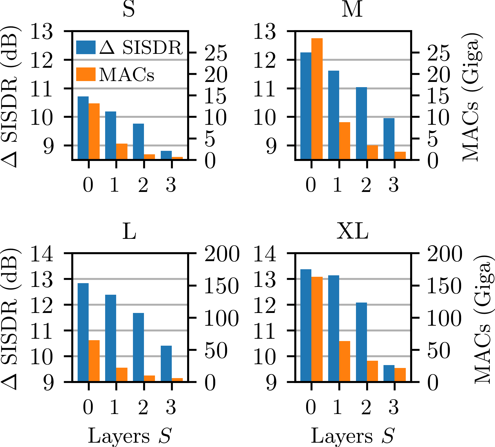
From Figure 7 it is notable that the difference in performance between $S=0$ and $S=1$ layers is less than between $S=1$ and $S=2$ and likewise then for $S=2$ and $S=3$. It is also noticeable that for the smaller model sizes the reduction in performance for each additional subsampling layer is also smaller. The $S=0$ configuration gives the best overall performance for both the S and XL TD-conformer models. This is expected as $S=0$ gives the MHSA layers in the conformer the highest temporal resolution when processing the global context. This improvement comes at a significant computational cost however as can be seen from the MACs reported in Figure 7 (note the scales vary for each row). This provides some justification for using a small number of subsampling layers at the benefit of significant reductions in computational requirements.

5.3 Hyper-parameter optimization and comparison to other models

In the following, TD-Conformer models are compared with several other discriminative supervised speech separation models. To find optimal configurations for the conformer models, a set of TD-Conformer models with $S=1$ subsampling layers and kernel sizes $P\in\{64,125\}$ are trained. Models with no subsampling ($S=0$) are not evaluated, due to unreasonably long training times on the hardware available for only minor improvements in performance (cf. Section 5.2). The kernel size $P=64$ was specifically chosen as it gives an equal RF to the optimal configuration $\{P,S\}=\{32,2\}$ in Section 5.1, cf. (6). DM, as implemented in [32], is also used to maximise model performance for each of the models. Results are reported with and without dynamic mixing (DM). MACs are reported for all models for which an open source implementation was available for evaluation [19, 26, 33, 10]. Performance in terms of $\Delta$ SISDR for the WSJ0-2Mix anechoic speech mixture dataset [29] is shown for completeness.

Table 1 shows that all TD-Conformer models outperform the STFT conformer model proposed in [13]. The small TD-Conformer-S models outperform the similarly sized and complex DTCN and SuDoRMRF++ baselines [33, 26] with DM on WSJ0-2Mix and show comparable performance on WHAMR without DM. The medium TD-Conformer-M models give comparable performance to the similarly sized SkiM baseline [34] on the WSJ0-2Mix benchmark but with less than half the number of MACs. The large TD-Conformer-L models give better performance than the SepFormer baseline on the WHAMR benchmark and comparable performance on WSJ0-2Mix with a similar model size but roughly a third of MACs. The TD-Conformer-XL model outperforms the much larger quasi-dual-path network (QDPN) model on WHAMR with the best model giving $14.6$ dB $\Delta$ SISDR. The TD-Conformer does not quite reach parity with the more recent MossFormer-L and TF-GridNet [35, 36] models however the largest TF-GridNet model has significantly higher computational expenditure and MossFormer is an augmented version of a Conformer model. Thus the results here help to validate the design choice of this approach.

		$\Delta$ SISDR (dB)
Model	$P$	W-2Mix	WHAMR	MACs	Params
Conv-TasNet [19]	-	15.6	9.7*	3.6G	5.1M
STFT-Conformer [13]	-	10.8*	6.7*	1.8G	57.5M
SuDoRMRF++ +DM [26]	-	17	-	2.7G	2.7M
DTCN [33]	-	15.6	10.2	3.7	3.6M
DTCN+DM [33]	-	17.2	11.1	3.7G	3.6M
SkiM [34]	-	18.3	-	19.7G	5.9M
SepFormer [10]	-	20.4	11.5*	60.7G	25.6M
SepFormer+DM [10]	-	22.3	14	60.7G	25.6M
QDPN [4]	-	22.1	13.1	-	200M
QDPN+DM [4]	-	23.6	14.4	-	200M
MossFormer-L+DM [35]	-	22.8	16.3	42.8G	42.1M
TF-GridNet (Tab. XIII) [36]	-	22.0	-	29.8G	6.8M
TF-GridNet [37, 36]	-	23.4	17.1	228.2G	14.3M
TD-Conformer-S	64	15.8	10.5	3.7G	1.8M
TD-Conformer-S	125	15.9	10.5	3.7G	1.8M
TD-Conformer-S+DM	64	17.4	9.7	3.7G	1.8M
TD-Conformer-S+DM	125	17.5	9.7	3.7G	1.8M
TD-Conformer-M	64	17.7	11.7	8.5G	6.7M
TD-Conformer-M	125	17.8	11.6	8.6G	6.8M
TD-Conformer-M+DM	64	18.1	12.0	8.5G	6.7M
TD-Conformer-M+DM	125	18.8	11.9	8.6G	6.8M
TD-Conformer-L	64	19.5	12.3	21.9G	25.9M
TD-Conformer-L	125	19.7	12.5	22.0G	26.2M
TD-Conformer-L+DM	64	20.3	13.4	21.9G	25.9M
TD-Conformer-L+DM	125	20.2	13.2	22.0G	26.2M
TD-Conformer-XL	64	20.4	13.1	63.6G	102.2M
TD-Conformer-XL	125	20.3	13.0	63.9G	102.7M
TD-Conformer-XL+DM	64	21.1	14.6	63.6G	102.2M
TD-Conformer-XL+DM	125	21.2	14.3	63.9G	102.7M

Table 1: $\Delta$ SISDR results for various TD-Conformer models with $S=1$ compared to other separation models on the WSJ0-2Mix (abbrev. W-2Mix) and WHAMR benchmarks. * indicates results not included in the respective paper cited for a model.

6 Conclusion

In this paper, a single-channel time-domain conformer speech separation model was introduced and evaluated. It was shown to reach comparable $\Delta$ SISDR performance as SOTA models on the WHAMR and WSJ0-2Mix benchmarks. Using conformer layers in place of DP transformer layers was demonstrated to reduce the TC of processing local information whilst increasing the TC for processing global context. A benefit of increased global TC is that it gives the global context layer a higher temporal resolution as demonstrated by varying the number of subsampling layers before the conformer layers in the proposed network. The proposed TD-Conformer-XL model achieves $14.6$ dB $\Delta$ SISDR on the WHAMR benchmark. The smallest TD-Conformer-S model outperforms a number of larger and similarly complex models on the WSJ0-2Mix and WHAMR benchmarks.

References

- [1] M. Kolbaek, D. Yu, Z.-H. Tan, J. Jensen, M. Kolbaek, D. Yu, Z.-H. Tan, and J. Jensen, “Multitalker speech separation with utterance-level permutation invariant training of deep recurrent neural networks,” IEEE/ACM Trans. Audio, Speech and Lang. Proc., vol. 25, no. 10, p. 1901–1913, Oct. 2017.
- [2] Y. Luo and N. Mesgarani, “TasNet: Time-domain audio separation network for real-time, single-channel speech separation,” in ICASSP 2018, Apr. 2018.
- [3] W. Ravenscroft, S. Goetze, and T. Hain, “Utterance weighted multi-dilation temporal convolutional networks for monaural speech dereverberation,” in IWAENC 2022, Sep. 2022.
- [4] J. Rixen and M. Renz, “QDPN - Quasi-dual-path Network for single-channel Speech Separation,” in Interspeech 2022, Sep. 2022.
- [5] R. Haeb-Umbach, J. Heymann, L. Drude, S. Watanabe, M. Delcroix, and T. Nakatani, “Far-Field Automatic Speech Recognition,” Proceedings of the IEEE, vol. 109, no. 2, pp. 124–148, 2021.
- [6] N. Moritz, M. Schädler, K. Adiloğlu, B. Meyer, T. Jürgens, T. Gerkmann, B. Kollmeier, S. Doclo, and S. Goetze, “Noise Robust Distant Automatic Speech Recognition Utilizing NMF based Source Separation and Auditory Feature Extraction,” in Proc. 2nd Int. Workshop on Machine Listening in Multisource Environments (CHiME 2013), 2013.
- [7] M. Maciejewski, G. Wichern, and J. Le Roux, “WHAMR!: Noisy and reverberant single-channel speech separation,” in ICASSP 2020, May 2020.
- [8] W. Ravenscroft, S. Goetze, and T. Hain, “Att-TasNet: Attending to Encodings in Time-Domain Audio Speech Separation of Noisy, Reverberant Speech Mixtures,” Frontiers in Signal Processing, vol. 2, 2022.
- [9] J. Chen, Q. Mao, and D. Liu, “Dual-path transformer network: Direct context-aware modeling for end-to-end monaural speech separation,” in Interspeech 2020, Oct 2020.
- [10] C. Subakan, M. Ravanelli, S. Cornell, M. Bronzi, and J. Zhong, “Attention is all you need in speech separation,” in Interspeech 2021, July 2021.
- [11] K. Li, R. Yang, and X. Hu, “An efficient encoder-decoder architecture with top-down attention for speech separation,” in ICLR 2023, May 2023.
- [12] Y. Luo, Z. Chen, and T. Yoshioka, “Dual-path RNN: efficient long sequence modeling for time-domain single-channel speech separation,” in ICASSP 2020, Oct 2019.
- [13] S. Chen, Y. Wu, Z. Chen, J. Wu, J. Li, T. Yoshioka, C. Wang, S. Liu, and M. Zhou, “Continuous speech separation with conformer,” in ICASSP 2021, Jun. 2021.
- [14] T. Cord-Landwehr, C. Boeddeker, T. von Neumann, C. Zorila, R. Doddipatla, and R. Haeb-Umbach, “Monaural source separation: From anechoic to reverberant environments,” in IWAENC 2022, Sep. 2022.
- [15] R. Sinha, M. Tammen, C. Rollwage, and S. Doclo, “Speaker-conditioning single-channel target speaker extraction using conformer-based architectures,” in IWAENC 2022, Sep. 2022.
- [16] E. Kim and H. Seo, “SE-Conformer: Time-Domain Speech Enhancement Using Conformer,” in Interspeech 2021, 2021.
- [17] W. Ravenscroft, S. Goetze, and T. Hain, “Receptive Field Analysis of Temporal Convolutional Networks for Monaural Speech Dereverberation,” in EUSIPCO 2022, Aug. 2022.
- [18] D. Ditter and T. Gerkmann, “A multi-phase gammatone filterbank for speech separation via tasnet,” in ICASSP 2020, 2020.
- [19] Y. Luo and N. Mesgarani, “Conv-TasNet: Surpassing ideal time–frequency magnitude masking for speech separation,” IEEE/ACM Transactions on Audio, Speech, and Language Processing, vol. 27, no. 8, pp. 1256–1266, 2019.
- [20] A. Gulati, J. Qin, C.-C. Chiu, N. Parmar, Y. Zhang, J. Yu, W. Han, S. Wang, Z. Zhang, Y. Wu, and R. Pang, “Conformer: Convolution-augmented Transformer for Speech Recognition,” in Interspeech 2020, Oct. 2020.
- [21] L. J. Ba, J. R. Kiros, and G. E. Hinton, “Layer normalization,” 2016. [Online]. Available: https://arxiv.org/abs/1607.06450
- [22] S. Elfwing, E. Uchibe, and K. Doya, “Sigmoid-weighted linear units for neural network function approximation in reinforcement learning,” Neural Networks, vol. 107, pp. 3–11, 2018.
- [23] G. E. Hinton, N. Srivastava, A. Krizhevsky, I. Sutskever, and R. R. Salakhutdinov, “Improving neural networks by preventing co-adaptation of feature detectors,” 2012. [Online]. Available: https://arxiv.org/abs/1207.0580
- [24] Y. Wu and K. He, “Group normalization,” in ECCV 2018, Sep 2018.
- [25] A. Vaswani, N. Shazeer, N. Parmar, J. Uszkoreit, L. Jones, A. N. Gomez, Ł. Kaiser, and I. Polosukhin, “Attention is All you Need,” in Advances in Neural Information Processing Systems, I. Guyon, U. V. Luxburg, S. Bengio, H. Wallach, R. Fergus, S. Vishwanathan, and R. Garnett, Eds., vol. 30. Curran Associates, Inc., 2017.
- [26] E. Tzinis, Z. Wang, X. Jiang, and P. Smaragdis, “Compute and memory efficient universal sound source separation,” Journal of Signal Processing Systems, vol. 94, no. 2, pp. 245–259, Feb 2022.
- [27] W. Ravenscroft, S. Goetze, and T. Hain, “On Data Sampling Strategies for Training Neural Network Speech Separation Models,” in EUSIPCO 2023, Sep. 2023.
- [28] J. Le Roux, S. Wisdom, H. Erdogan, and J. R. Hershey, “SDR – Half-baked or Well Done?” in ICASSP 2019, May 2019.
- [29] Y. Isik, J. Le Roux, Z. Chen, S. Watanabe, and J. R. Hershey, “Single-Channel Multi-Speaker Separation using Deep Clustering,” in ICASSP 2016, Sep. 2016.
- [30] M. Ravanelli, T. Parcollet, P. Plantinga, A. Rouhe, S. Cornell, L. Lugosch, C. Subakan, N. Dawalatabad, A. Heba, J. Zhong, J.-C. Chou, S.-L. Yeh, S.-W. Fu, C.-F. Liao, E. Rastorgueva, F. Grondin, W. Aris, H. Na, Y. Gao, R. De Mori, and Y. Bengio, “Speechbrain: A general-purpose speech toolkit,” 2021. [Online]. Available: https://arxiv.org/abs/2106.04624
- [31] “Thop: Pytorch-opcounter,” https://pypi.org/project/thop/, accessed: 19-10-2022.
- [32] N. Zeghidour and D. Grangier, “Wavesplit: End-to-end speech separation by speaker clustering,” IEEE/ACM Transactions on Audio, Speech, and Language Processing, vol. 29, pp. 2840–2849, 2021.
- [33] W. Ravenscroft, S. Goetze, and T. Hain, “Deformable temporal convolutional networks for monaural noisy reverberant speech separation,” in ICASSP 2023, Jun. 2023.
- [34] C. Li, L. Yang, W. Wang, and Y. Qian, “Skim: Skipping memory lstm for low-latency real-time continuous speech separation,” in ICASSP 2022, May 2022.
- [35] S. Zhao and B. Ma, “Mossformer: Pushing the performance limit of monaural speech separation using gated single-head transformer with convolution-augmented joint self-attentions,” in ICASSP 2023, Jun. 2023.
- [36] Z.-Q. Wang, S. Cornell, S. Choi, Y. Lee, B.-Y. Kim, and S. Watanabe, “TF-GridNet: Integrating full- and sub-band modeling for speech separation,” 2022. [Online]. Available: https://arxiv.org/abs/2211.12433
- [37] ——, “TF-GridNet: Making time-frequency domain models great again for monaural speaker separation,” in ICASSP 2023, Jun. 2023.