Waiting for Inflation: A New Initial State for the Universe
Abstract
We propose a cosmological lingering phase for the initial state prior to inflation which would help address the singularity problem of inflation. The universe begins with a constant (Hagedorn) temperature and then transitions into an inflationary universe while preserving the Null Energy Condition (NEC). In such a universe time is presumably emergent, calling the age of the universe into question. We first consider the phase space of positive spatial curvature models within General Relativity and with matter sources that respect the NEC. Depending on the duration of the post-lingering inflation these models can produce a small amount of observable spatial curvature in the Cosmic Microwave Background. We also discuss how lingering can arise with or without spatial curvature in theories of quantum gravity when considering the thermodynamic scaling of particles and its impact on the early universe. The string theory dilaton is essential to the dynamics. There are many open questions that remain.
I Introduction
Cosmological inflation Guth (1981); Linde (1982); Albrecht and Steinhardt (1982) provides a theoretically motivated paradigm for the origin of large scale structure, the origin of anisotropies in the Cosmic Microwave Background (CMB) and an explanation for a number of puzzles about the initial conditions for the ’Big Bang’. In this paper, we present the background evolution of a lingering universe that leads to cosmological inflation – emphasizing that this does not violate the Null Energy Condition (NEC). In addition, we show that perturbations in the hydrodynamical fluids sourcing the background evolution grow during the lingering phase (which we will present in more detail in a second paper), before the transition to the inflationary phase. Since Cosmic Microwave Background (CMB) measurements provide the amplitude of inhomogeneities at a given scale Akrami et al. (2018), any growth of perturbations in the lingering phase must be compensated by a corresponding decay in the period following the lingering. It is important to note that since lingering demands the existence of positive curvature (i.e. the universe is closed), we will already have a lower bound on the duration of inflation. The matching of inhomogeneities will provide a further restriction on the duration of lingering and inflation.
A lingering phase in cosmic evolution was first consider by Lemaitre Lemaître (1931) while investigating the dynamics of a closed universe with a cosmological constant. Such a phase was reconsidered in more “recent” times to address the age problem, i.e. a discrepancy in determining the age of the universe when comparing observations of the Hubble to the age of the oldest globular clusters. A similar type phase was suggested to provide a late-time mechanism for generating large scale structure (following matter domination) and could also lead to late-time cosmic acceleration Sahni et al. (1992). With improving observations and the successful predictions of inflation, the late lingering (loitering) universe fell out of favor. However, as we discuss more below, such a phase is feasible for the very early universe and then leads to inflation.
II A Lingering Universe in Classical Gravity
We begin by considering the Friedmann, Lemaître, Robertson, and Walker (FLRW) metric for a homogeneous and isotropic universe
| (1) |
allowing for spatial curvature . Introducing the Hubble parameter and allowing for a cosmological constant the Einstein equations can be written as
| (2) | |||||
| (3) |
where . Combining the above equations we get the Friedmann equation
| (4) |
The energy density and pressure obey the continuity equation111If we think of the cosmological constant term as a fluid we would have so that has units of mass squared. Similarly, we could think of spatial curvature (mathematically) as an energy density with pressure and is the critical density in spatial curvature.
| (5) |
The above equations were considered in various limits in the early days of cosmology to address observations of extragalactic ‘nebulae’ (see Table I). A particularly interesting account was given by Lemaître Lemaître (1931) to resolve an issue between models of de Sitter and Einstein. The upshot of that work was that the universe must expand in the presence of matter and energy and these static solutions are unstable. In modern terminology we can recast (2) as
| (6) |
where is a constant value for the Hubble parameter (typically taken as its value today) when , and ’s are the corresponding critical densities in the cosmological constant, radiation, matter, and curvature respectively. These values have been determined with great precision Aghanim et al. (2020) demonstrating – among other things – that a constant value of the Hubble parameter is not consistent with General Relativity.
| a(t) | K | Ricci Scalar | Description | ||
|---|---|---|---|---|---|
| 0 | 0 | 0 | 0 | Minkowski | |
| 0 | De Sitter (dS) | ||||
| 0 | 1 | 0 | Einstein Static Universe | ||
| +1 | Lemaître (a.k.a. lingering) |
In the remainder of this paper we revisit some of these solutions. Firstly, it is important to note that some of these ‘states’ for the universe can be realized as asymptotic fixed points of the dynamic flow from one state of the universe to another as time evolves – we make this more precise below. As an example, if inflation is past-eternal it is typically assumed that this would lead asymptotically to dS space-time in the distant past. This would again imply that the universe began in a singularity (as in the standard Big Bang theory) as it is expected dS is geodesically incomplete in its infinite past implying the existence of a true singularity Borde et al. (2003) – for a more recent analysis we refer to Kinney et al. (2023). We also note that bouncing universes, such as the Cyclic / Ekpyrotic universes have also been shown to suffer from these issues Kinney and Stein (2022).
Moreover, many of the examples in Table I correspond to models with non-trivial spatial curvature. Spatial curvature is typically neglected in model building because the observationally determined value today from CMB, lensing, and BAO measurements is Aghanim et al. (2020). However, it is also interesting that in the 2018 Planck results Aghanim et al. (2020) it was suggested that a non-zero spatial curvature might be favored by the data222There are many degeneracies in the data and we are in no way stating there is strong evidence for this. Further data will help clarify the situation..
II.1 Dynamics in a lingering Universe
In what follows it will be useful to work in conformal time and we will consider matter and energy with equation of state , where with is the pressure and is the energy density of the -th fluid. We will consider two types of fluids, one that is Standard Model-like , and another that scales slower than curvature with . The equations for the background are
| (7) | ||||
| (8) |
where is the conformal Hubble parameter, is the total energy density of the multiple sources and is the corresponding total pressure. We will find it more convenient to rescale our space-time co-ordinates by the spatial curvature. We can do this without changing the form of (7) and (8) since the FLRW metric is invariant under the scaling
This means we can choose such that we work with variables , etc333Note that this means our scale factor now carries units of length, while our co-ordinates are unitless. Typically, one then uses the notation for the scale factor, but we use for the sake of vexation.. We drop the tildes in what follows unless more context is necessary. Solutions follow from solving (7) and (8) with , along with the continuity equation for each fluid
| (9) |
Assuming a constant equation of state for each fluid the energy density scales as . Using (7) in (8) we have
| (10) |
Another useful combination of (7) and (8) results in a second-order equation for the scale factor
| (11) |
The Lingering Fixed Point
A strictly lingering phase corresponds to a constant scale factor and vanishing Hubble parameter. While in conformal time we have , the conformal Hubble radius diverges. Using (10) and (11) a lingering phase implies
| (12) | |||
| (13) |
where corresponds to standard matter and radiation, and corresponds to an additional sector with , which does not violate the NEC. We use a bar to represent these quantities in the strictly lingering phase. For later convenience we have defined and , which are related to the scaling and in the case of constant equation of state. The constraints then imply and . We emphasize that the conditions (12) and (13) are true for a strictly lingering universe where the first and second time derivatives of the scale factor vanish at all times.
As mentioned above, in Sahni et al. (1992) the authors considered a period of cosmic lingering. They were seeking lingering solutions at low red-shift (late in matter domination) to address discrepancies in measured values of from CMB observations and those from clustering444It may be interesting to revisit this idea to address the current Hubble tension.. They also considered if their model could provide a possible mechanism for dark energy. To do this they decided upon initial conditions based on observations that would give appropriate amounts of spatial curvature, exotic matter, and clustering matter. Given these considerations they determined at which specific red-shift the universe must linger.
Our approach here is very different – we want to impose lingering as an initial condition for the beginning of inflation. Thus, rather than finding specific values of and the scale factor such that the universe stalls, we determine the values of and that are allowed by a given scale factor and curvature. We find that for
| (14) |
the universe will linger at scale factor . Notice that our assumptions on the equations of state imply that both energy densities remain positive .
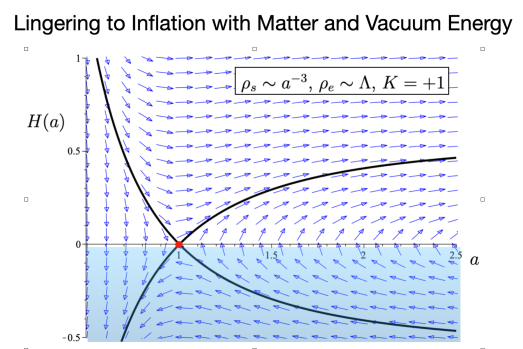
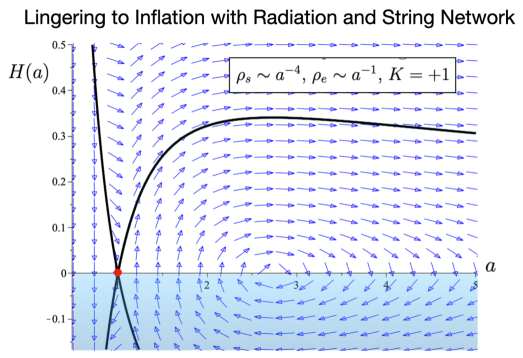
We should immediately note that the case is special. In that case, the universe can linger at any scale factor as long as and . The resulting dynamics can be seen from the phase space plots in Figures 1 and 2. The first figure illustrates the flow for a universe from lingering in the presence of matter and vacuum energy, asymptotically leading to inflation. Positive spatial curvature is essential for this solution to be consistent. Figure 2 is an alternative situation where we consider radiation and a cosmic string network – again leading to inflation. An important question we cannot answer is the duration of the lingering phase as we elaborate on below.
Our interest now lies in the amount of matter for which the lingering phase ends in a finite amount of time, i.e. and . We can characterize the length of the lingering phase by tracking “nearby” scale factor trajectories. To this end, we suppose that , and . If the additional sector scales like curvature ( corresponding to ) we must remember that the lingering amount of clustering matter is zero. In that case, we can’t parameterize the deviation of the energy density as a fraction of what is required for lingering. We must include two possible changes to the clustering matter: , where will vanish in the case. Expanding (7) and (8) to first order in the departure from lingering we have
| (15) | ||||
| (16) |
The first of these equations ensures that . Assuming the new trajectory exactly matches the perfect lingering solution at some starting point , the above equations are solved by
| (17) |
where . When the resulting equations are instead
| (18) | ||||
| (19) |
which is easily solved for
| (20) |
Note that one can pass from the solution to the solution via the formal limit .
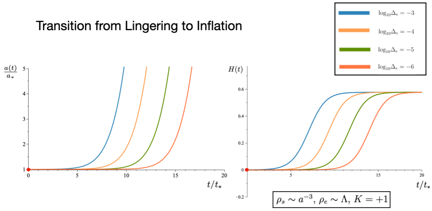
Of course, this linear approximation breaks down when approaches one; this signals the exit from the lingering phase. Via inspection of the solutions above, one finds that with energy densities closer to their exact lingering values, the longer the duration of the quasi-lingering phase lasts. This is shown in fig. 3. We can estimate the end of lingering as
| (21) |
when . We assumed that to arrive at the above expression. When ,
| (22) |
Both of these time durations obey for , which is the perfectly lingering limit.
To this point, we made no assumptions on , , or . The forms of (15) and (18), as well as the interesting ranges for and , require the changes in the energy density of the fluids to be opposite-signed. The universe, desiring to stall at the same scale factor as in its perfect lingering form, must compensate any additional energy in a given fluid by a corresponding loss in the other. Simple inspection of the solutions to the deviated lingering equations reveals that when we have reduced the amount of energy in the additional sector, the universe tends to recollapse, as expected for a closed universe filled with standard matter.
The case introduces further complications that necessitate extra elucidation. Note that the perfect lingering scenario requires zero standard matter to achieve a steady-state universe. Thus, any additional matter sector inserted to break lingering requires the corresponding reduction of standard matter. In other words, the universe needs negative energy density in the standard matter sector to obtain an initially lingering solution followed by an exponentially expanding inflation-like solution.
We note that these considerations qualitatively and quantitatively change the nature of the post-lingering behavior of the scale factor. Below, we consider the universe to be dominated by the additional sector fluid after lingering, a fact which depends on the additional sector diluting slower, with cosmic expansion, than the standard matter. If, instead of continuing to expand, the universe shrinks, the reverse situation holds. With cosmic contraction, standard matter concentrates faster than the additional sectors. It would only be a short time before the standard matter dominated over the additional sector. Since our current universe appears to be expanding at an accelerated rate, we ignore the options of collapsing universe in what follows.
II.2 Post-lingering and the Exit to Inflation
By their scaling, matter and radiation dilute with the cosmic expansion faster than the dS-like sector. Neglecting the matter sector then provides us with the equations that determine the evolution of the scale factor in the post-lingering era. In this limit, (11) takes the form
| (23) |
where we have inserted the ansatz for discussed above. The first Friedmann equation then takes the form
| (24) |
The above equations can be solved for for the relevant values of . We denote by the conformal time duration since the post-lingering transition. The general solution for (23) and (24) is
| (25) |
where is the remaining constant of integration set by initial value of the scale factor at the start of the post-lingering phase of evolution From this solution, it is clear that we need to treat the case separately. For , using the exponentially expanding solution of (23) in (24), we find
| (26) |
where is the scale factor at the the lingering to post-lingering transition.
III Cosmology from a Hagedorn Phase
In this section, we present the motivation from string theory for an initial phase of cosmological lingering. We then demonstrate how this can lead to a period of inflation without a NEC violating transition. In regards to the presentation thus far, within the context of string theory (quantum gravity) we address the question: Is spatial curvature an essential component for a NEC preserving, lingering universe555Spoiler Alert: Our results respect Betteridge’s law of headlines.? We also discuss how our approach relates and differs from previous considerations in the literature.
III.1 Model Independent String Cosmology
Essentially all string theory compactifications give rise to the following terms in the effective action (written in the four-dimensional string frame) Polchinski (2007); Green et al. (1988a, b):
| (27) | |||||
where (for simplicity) we have assumed a string compactification from ten to four dimensions ( is the volume of the extra dimensions in string units), is the string frame metric, is the corresponding Ricci scalar, is the string coupling, and is the string scale. We have focused on the bosonic string spectrum assuming weak coupling and small space-time curvature. We have also neglected fermions, tachyons, critical dimensions, world-sheet curvature, Ramond - Ramond fluxes, and the possibility of supersymmetry as including these effects would not alter our main conclusions. However, we have included a term which can account for arbitrary sources of the dilaton. Finally, is the three-form flux (an Einstein - Maxwell field) and a scalar field – the dilaton.
Given our analysis in the previous sections, it will be useful to recast this theory in the Einstein frame. We emphasize that it is in the Einstein frame that one should invoke the NEC if one is interested in the stability of the theory and the presence of singularities. There is a notion of these issues in the string frame (physics does NOT depend on the frame, however the singularity theorems were originally formulated in the Einstein frame Hawking and Ellis (2023), and are most easily interpreted in the context of General Relativity666One can consider the NEC in both frames but it is simpler to interpret in the Einstein frame Gasperini and Veneziano (1993a) where violations can be interpreted through energy and matter following geodesics in a clear way as originally stated by Hawking and Ellis Hawking and Ellis (2023).. In the four-dimensional Einstein frame, defined by the conformal transformation (which does not affect experimental observations)
| (28) |
(27) becomes
| (29) |
where as in previous sections, and the fields and have been rescaled, the gravitational term has the usual Einstein-Hilbert form, and the dilaton source now has dilaton dependent coupling. Except in Type I string theory, is the four-dimensional part of the field strength of the Neveu-Schwarz two-form, and is defined via the equation . The dilaton and the axion are common to nearly all string theories and this simple model captures many aspects that string compactifications and the resulting cosmologies have in common. We might immediately suppose that there are FLRW solutions where approximately describes a semi-circular geodesic in the upper half plane (with a relevant field-space metric), and that by making small, we can avoid significant back-reaction of the scalars on the geometry. Again, the action becomes more involved in the presence of supersymmetry (and its breaking), additional fields, branes, extra dimensions, etc. – but these can (and have) been accounted for in the literature to a large extent (see e.g. Silverstein (2004); Kane et al. (2015)). Here we will focus on the dimensional cosmologies as we did above, and in the simplest terms to reach our conclusions.
The role of in string theory is played by the Vacuum Expectation Value (VEV) of the dilaton, which is related to the string coupling and in the dimensionally reduced theory this would also include the extra dimensions as expressed in (27). The the role of gravitational corrections are controlled by the string scale – which here we will take parametrically below the Planck scale (). In particular, the Planck scale is a derived quantity which involves: the dynamics of the dilaton (its resulting VEV), the value of the string scale, and the size and dynamics of any extra dimensions (here assumed six-dimensional777Strictly speaking, string theories do not require 10 or 11 dimensions to be consistent, nor do they require supersymmetry Polchinski (2007); Green et al. (1988a, b). This may be an important clue on how to realize realistic models of cosmology from string theory – such as quasi- but not exact dS space-time Hellerman et al. (2001). ). An important consequence of this is that when one considers decoupling limits one must take into account the other scales (and dynamics) involved. Looking into these consequences has led to interesting conjectures – such as the Weak Gravity conjecture and notion of the Swampland of quantum field theories Ooguri and Vafa (2007); Vafa (2005); Ooguri et al. (2019); Garg and Krishnan (2019).
Moreover, string theory comes with a number of dualities Polchinski (2007); Green et al. (1988a, b) resulting from the worldsheet theory and manifested in the low-energy action (27). These symmetries can be used to relate the weak coupling limit of one realization of the theory with the strong coupling of another. When applied to the geometry they also imply a theoretical correspondence between the large volume limit of one theory with the small volume limit of another theory. Finally, when applied to cosmology this would imply a ‘scale-factor’ duality Brandenberger and Vafa (1989); Veneziano (1991); Tseytlin and Vafa (1992). Given the latter, string theory was used to motivate alternatives to standard inflation resulting from a bouncing universe – examples include String Gas Cosmology (SGC) Brandenberger and Vafa (1989); Battefeld and Watson (2006) and the Pre-Big-Bang (PBB) Gasperini and Veneziano (1993a).
What we are not considering in this paper. In SGC and PBB models, the goal is to produce an alternative to standard inflation to resolve the classic issues of the background (the Horizon, flatness, entropy problems, etc.), while also (causally) generating cosmological perturbations to provide seed perturbations for the CMB and Large-scale Structure888One possible exception to this appears in Kamali and Brandenberger (2020). However, our approach differs in that those authors again considered a bouncing cosmology in the context of SGC that then led to inflation.. One challenge for these approaches is that they invoke a ‘bounce’ before or near the cosmological singularity, and in perturbation theory (required to trust the effective action (27)) this implies a violation of the NEC. Also, as mentioned above such approachs can also suffer from singularity issues as established in Borde et al. (2003); Kinney et al. (2023); Kinney and Stein (2022). We will return to these points, but first we further discuss the motivation for a new phase of early universe cosmology – a lingering phase.
III.2 The Hagedorn Phase
In addition to (27), another robust prediction of string theories is their thermodynamic properties at high energy. An important first step for understanding the high temperature behavior resulted from considerations of Hagedorn while exploring quark deconfinement and its dependence on temperature in Hagedorn (1965). In particular, this study led Hagedorn to the idea of a cosmic and phenomenological limiting temperature. Such thermodynamical behavior signals a departure from standard QFT, the partition function will have an exponentially diverging degeneracy of states (hence the mass spectrum) at high energy and temperatures. When interpreted within string theory, this implies a maximum temperature for a fluid of strings – the so-called Hagedorn temperature Atick and Witten (1988).
Cosmologically, the epoch in which the limiting temperature is achieved, , implies a phase where the temperature remains roughly constant – a result from the fact that the energy of a string does not increase Atick and Witten (1988). Naively, for FLRW cosmology this would imply that a gas of strings would evolve like pressure-less matter – with constant. However, an important consideration is the string dilaton, which would also be present within string theory Tseytlin and Vafa (1992). The resulting dynamics implies a departure from standard FLRW intuition as manifested in the String frame (27). Moreover, in addition to the Hagedorn phase and the dilaton, string theory also generically leads to extra dimensions and ‘winding strings’. In a simple realization, we can consider extra dimensions in the form of a six-dimensional torus (a simple example of a Calabi-Yau manifold) with strings wrapping the cycles of these dimensions999We note that this may seem rather exotic to the unfamiliar, however the extra dimensions can also be used to understand important problems in particle phenomenology and cosmic inflation – where it has been crucial in providing a systematic way to calculate corrections to the low-energy effective field theory. in addition to unwrapped strings (particles – the low energy states being the graviton, Einstein-Maxwell fields (model independent axions), and the dilaton). A cosmological consequence of the dilaton and the wrapped states is they don’t lead to inflation (as in standard FLRW) but instead preserve the Hagedorn phase dynamics.
To study the dynamics we start by considering a homogeneous but anisotropic metric
| (30) |
where is the lapse function which we gauge fix to 1 in what follows, are string frame scale factors for the spatial directions. Specializing to isotropic cosmologies () with , the equations of motion resulting from (27) are
| (31) |
where and are the string frame energy density and pressure, is the string scale Hubble parameter, and is the variational derivative of with respect to the dilaton, which we set to zero for now. We work in units . We note that these equations become the same as the Einstein frame equations in Section II if when we take the (unshifted) dilaton to be constant and include spatial curvature through the energy density. The energy and pressure of sources are defined in the string frame and given by101010See Kaloper and Watson (2008) for more detail. the comoving free energy as
| (32) |
where is the inverse temperature and . The sources obey the conservation equation
| (33) |
We will focus on the sources of the form with equation of state parameter , and are the energy and pressure density derived from the comoving quantities and respectively. Given the considerations above, we will be interested in two cosmological phases. One phase corresponds to the Hagedorn phase of strings where their energy does not increase and the temperature remains nearly constant. This implies an equation of state for the Hagedorn phase – . Whereas, below the Hagedorn phase (but still at relatively high temperatures ) strings have two types of scaling behavior111111One may ask about the importance of string oscillations, but it has been shown that these can be neglected relative to the sources we consider Kripfganz and Perlt (1988). corresponding to radiation () and winding strings (). In both epochs we will see the dilaton plays a crucial role in the dynamics.
III.2.1 Cosmological Solutions
Solutions of the system (III.2) can be found for constant equation of state by introducing a time such that
| (34) |
where is a constant reference energy. Using (34) the equations (III.2) are equivalent to
| (35) | |||||
where primes denote derivative with respect to , is the shifted dilaton, and energy scales as .
Looking for isotropic solutions with constant equation of state one finds Gasperini and Veneziano (1993b),
| (36) | |||||
| (37) | |||||
| (38) |
with singularities at
| (39) |
where and , , , , and are integration constants. is a classically forbidden region.
III.2.2 Hagedorn Phase at
For the Hagedorn phase with , the energy density is dominated by a fluid with constant energy and vanishing pressure , so that , in which case equations 36-38 become
| (40) | |||||
| (41) | |||||
| (42) |
where we have set the integration constants so that and . Using (34), the solution in co-ordinate time is obtained by replacing with –
| (43) | |||||
| (44) | |||||
| (45) |
where (again, the moment of the singularity) and the string coupling is
| (46) |
From (III.2), we see there are two branches of solutions –
| (47) | |||||
| (48) |
corresponding to the sign of . Differentiating equations 43 - 45 gives
| (49) | |||||
| (50) |
As emphasized in Kaloper and Watson (2008), these solutions represent different superselection sectors of the theory and are topologically distinct solutions categorized by the sign of .
The solution branches are summarized in Table 2 where we present the
four physically distinct solutions.
| Region | Branch | Expansion | Shifted Dilaton | Dilaton |
|---|---|---|---|---|
| I | ||||
| II | ||||
| III | ||||
| IV |
Phase Space Analysis of the Hagedorn Phase. Here we want to understand the phase space of solutions for the Hagedorn Phase. To do this it is useful to introduce a co-ordinate transformation
| (51) |
(Note: in this section primes represent the derivative with respect to ). Then the equations are
| (52) | |||
Introducing and the above equations can be taken as a first order system with fixed points
| (53) |
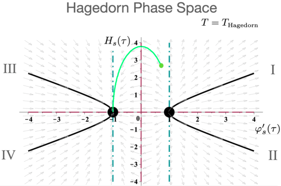
where is the sign of . Near the critical temperature as discussed earlier.
The phase space for Hagedorn cosmologies near the critical temperature is given in Figure 5. There we plot the string frame Hubble parameter in the conformal time versus the derivative of the shifted dilaton. All physically relevant trajectories are restricted by the Hamiltonian constraint (conservation of energy) to begin and end on the black (co-dimension one) hyperbolae. This is an important observation in that a trajectory that start in region I or II can not energetically go to region III or IV. We performed the conformal transformation to make this manifest (we also note this transformation is not singular). Thus, there are two distinct branches again separated by the sign of the shifted-dilaton. The green trajectory provides an example of an (unphysical) observer that respects the phase space flow but does not satisfy conservation of energy. The blue (dot-dash) trajectories are lines of constant (in conformal time) , whereas pink (dashed) trajectories correspond to constant (in conformal time) . Their intersection occurs at the causal (hyperbolic) fixed points of the phase space flow . In summary, our results agree with those of Kaloper and Watson (2008).
In appendix A we discuss how the Hagedorn phase in the string frame relates to that in the Einstein frame.
III.3 Post-Hagedorn Phase
We now turn to the cosmology when the temperature has decreased below the Hagedorn temperature. Such behavior is expected due to the fact that the lingering solution of the Hagedorn phase is a hyperbolic (unstable) fixed point for as can be seen from Figure 5. We will see in the next section that these solutions are the ones of interest for lingering cosmologies that respect the NEC. As mentioned above the stringy nature of particles will manifest itself as both radiation and string winding modes below the Hagedorn temperature – and the dilaton will play a crucial role until stabilized. From the discussion above, we can use the solutions from (36)-(38) where we have for radiation (winding modes). The solutions are
| (54) | |||||
| (55) | |||||
| (56) |
where again we set and . The upper sign in (54) corresponds to radiation (momentum modes) and the lower sign to winding modes. When considering the behavior far from the singularities (i.e. ), the energy for the momentum modes is given by , and noting the relation to the original co-ordinate time, we find that and the solutions in this limit approach
| (57) | |||||
| (58) | |||||
| (59) |
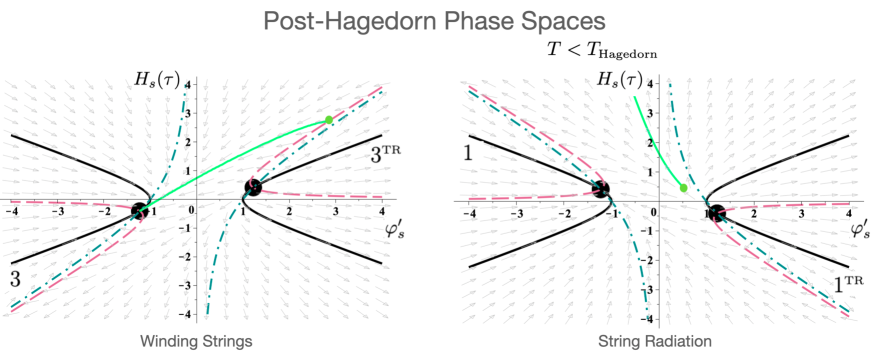
which is the standard FLRW radiation dominated universe. In general, the radiation phase leads to four physically distinct solutions which are expressed in Table 3. Likewise, we can find the solutions for the winding strings using T-duality, and oscillations of the strings can be neglected cosmologically. For more details we refer the reader to Kaloper and Watson (2008). Here we want to emphasize the analysis of the phase space.
| Region | Branch | Expansion | Shifted Dilaton |
|---|---|---|---|
| 1 | |||
| 3 | |||
To analyze the phase space of the sub-Hagedorn regime we again use the time redefinition (51) with for radiation / winding strings. Then the equations are given by (52) with the relevant values of . We again introduce and and the equations can be taken as a first order system with fixed points given by (53).
The phase spaces are given in Figure 6. There we plot the string frame Hubble parameter in the conformal time versus the derivative of the shifted dilaton. All physically relevant trajectories are restricted by the Hamiltonian constraint to begin and end on the black (co-dimension one) hyperbolae and any branch change would violate the conservation of energy. The green trajectory provides an example of an (unphysical) observer that respects the phase space flow but does not satisfy conservation of energy. The blue (dot-dash) trajectories are lines of constant (in conformal time) , whereas pink (dashed) trajectories correspond to constant (in conformal time) . Their intersection occurs at the causal (hyperbolic) fixed points and corresponding to the phase space flow of winding strings and radiation, respectively. We note that the mirror symmetry of the two plots is an example of T-duality in the theory.
IV Exit from lingering and the Null Energy Condition
In this section we review the importance of the egg function121212We would like to emphasize that no chickens were harmed in performing this research, however our eggs are not free range due to the constraints of the NEC. in describing violations of the NEC and the viability of models. The importance of this constraint is that NEC violations imply fine-tuning in cosmological models. Inflation does not have this type of fine-tuning, but does have a past singularity (geodesic incompleteness) Kinney and Stein (2022); Kinney et al. (2023) which, again, is what we are trying to address in this paper. We discuss both the classical model with spatial curvature (Section II) and the Hagedorn motivated model (Section III).
Considering whether a cosmological model violates the NEC is important for determining its viability and predicability. NEC violations signal the presence of cosmological singularities and a breakdown of General Relativity Hawking and Ellis (2023). In the context of the evolution of cosmological perturbations NEC violations are not detrimental, a priori, but imply the presence of fine-tuning of initial conditions especially when considering causality of observers Adams et al. (2006) and the evolution of cosmological perturbations. NEC violations do not have to be catastrophic, if localized in space-time and in a controlled manner respecting the limited range of validity of the effective field theory Creminelli et al. (2006). However, for a complete picture of the universe we will need to assume that the NEC is respected globally.
In the absence of a complete theory of quantum gravity we are forced to assume what is to be known as ‘reasonable’ properties of matter and energy. A conservative assumption is that sources should lead to positive or zero curvature so that geodesics of the space-time converge along a null vector (matter / energy is always attractive) Hawking and Ellis (2023). This null convergence condition requires , using Einstein’s equation this implies
| (60) |
For the FLRW type universes we are considering here, this implies .
In our analysis thus far, we have respected the NEC as we required our second sector to respect as discussed in Section II.1. In particular, the lingering conditions were
| (61) | |||
and these preserve the NEC at all times but also lead to interesting dynamics due to the presence of spatial curvature.
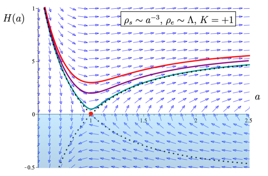
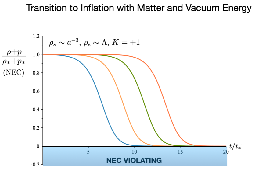
Indeed, as can be seen from Figure 7 the spatial curvature term leads to a saturation of the NEC as can also be deduced from the equations above.
Our classical analysis of Section II implies that the lingering phase can:
-
•
Be realized in a universe with positive spatial curvature while preserving the NEC,
-
•
Can exit to a period of inflation without violating the NEC.
We now turn to the analysis in Section III and review the challenges for a String Gas approach as discussed in Kaloper and Watson (2008).
IV.1 Branch change and the egg function
We reconsider the equations (III.2), now allowing for additional contributions that could arise from other stringy matter, or corrections, spatial curvature, etc. which may be non-trivially coupled to the dilaton. These can be included in the effective Lagrangian and in order to preserve spatial isotropy these sources must be of the perfect fluid form131313Although we consider the isotropic case here, given our assumption of spatial homogeneity the presence of anisotropy will not change our conclusions. As discussed in e.g. Brustein and Madden (1997), we could equivalently work in the effective theory and then the anisotropies would simply appear as sources in the effective ‘matter’ lagrangian. For our arguments to follow, it is enough to note that such sources (anisotropies) will not violate the Null Energy Condition., namely . We rewrite equations (III.2)
| (62) | |||||
| (63) | |||||
| (64) |
where results from the possible coupling of sources to the dilaton. Combining the above we find an equation that will prove useful below,
| (65) |
From (62) we immediately see that in order for a branch change to occur the so-called egg function
| (66) |
must vanish, implying that is required. Hence, the sign of acts as a kind of topologically conserved charge, in the sense that for positive energy solutions a branch change cannot occur classically.
One might optimistically hope that the addition of string corrections, non-trivial coupling to the dilaton, and/or other contributions to the effective action that appear in might allow for and a successful exit from the Hagedorn phase. Entertaining such a possibility let us continue assuming that is achieved and ask whether this is sufficient to achieve an exit from the Hagedorn phase.
A useful relation can be found by using and (65),
| (67) | |||||
| (68) |
where in the last step we have used the definition of the egg function (66) and the fact that as we approach the egg (). refers to the branch on which this evolves.
First let us consider the case when the sources are trivially coupled to the dilaton in the string frame, so that . We are interested in the possibility that we initially approach the egg from the Hagedorn branch and then make a transition to the RDU branch. Because we have seen that requiring analyticity implies (classically allowed region), it follows that in order for the transition to occur. In the case of trivial dilaton coupling (i.e. =0) we find
| (69) |
where we have used before the transition. We immediately see that a branch change cannot occur, since the egg is repulsive, i.e. the point is a repeller in the phase space and trajectories will not lead to successful transitions.
Let us now consider the case of non-trivial coupling to the dilaton. From branch solutions of (67), we might naively expect that a branch change could occur if contributions from are negative enough to change the overall sign. We will now show that is not the case, and will prove a no-go theorem for the Hagedorn exit.
IV.2 A no-go theorem for Hagedorn exit
Using (63), we eliminate from (67) giving
| (70) |
We integrate the above equation from the moment of the branch change when , to the moment of escape when ( thereafter) and . For evolution along the branch, this gives
| (71) |
Evaluating the integral, we find
| (72) |
where is the positive definite volume in the phase space. The left hand side is always positive, since on both branches. This implies that an exit from the Hagedorn phase requires , i.e., a violation of the NEC. One way to avoid this constraint is to introduce spatial curvature as we discussed in the ‘classical situation’. In previous results of String Gas Cosmology spatial curvature was ignored because inflation did not take place (it was posed as an alternative to inflation). But considering a lingering phase leading to inflation means that this is no longer an issue and could resolve the problems with NEC violation that we have discussed above.
In the string based models we are discussing here, they would simply start in the lingering phase and then evolve into dilaton led inflation. This can be seen from Figure 5. The phase space flow leads to a repeller (hyperbolic) fixed point, which then leads to inflation – there is no branch change. There are many open questions we must address. How long does loitering last – how does inflation end? These are challenging questions we must address in future research. The promising aspect of this work is it suggests a new way to look at the beginning of inflation.
V Conclusions
What we are not proposing. In the models we have presented above we considered solutions where the cosmological evolution moves toward a state of inflationary cosmology (quasi-dS space-time). That is, thus far we are relying on inflation to address the horizon, relic, flatness, etc… problems Guth (1981); Linde (1982); Albrecht and Steinhardt (1982). We are not proposing a complete alternative to inflation. Instead, we are proposing an alternative way to look at the beginning of inflation – the universe lingered. For minimal inflation there is an interesting possibility of small, but non-zero spatial curvature which would be clarified by CMB-S4 Abazajian et al. (2016) and other future observations. The motivation for this approach was to provide a new way to address the past cosmological singularity of inflation and the initial state of the universe. In future work we will consider the effect (if any) on the cosmological perturbations in the model.
We discussed a more provocative motivation in Section III. In string theory approaches to early universe cosmology, string dynamics can lead to a Hagedorn phase which cosmologically implies a lingering phase. As discussed above, the lingering phase does not demand the presence of spatial curvature and can instead arise from the dynamics of a string gas and an evolving dilaton. Thus far, the only known solution that would not violate the NEC naturally leads to inflation, as shown in Kaloper and Watson (2008). Our analysis here has used spatial curvature as a proxy for the string dynamics discussed above which will be considered in future work.
We have seen that the initial state of the universe can differ from that of a dS space-time and then evolve into an inflationary state without violating the Null Energy Condition. This suggests a new class of models for addressing the problem of initial conditions for inflation and related issues. In particular, the lingering phase and transition are motivated by the Hagedorn phase of string theory when applied to cosmology. Although this shares many similarities with models of String Gas Cosmology, it differs in that the transition from the initial state is to inflation and this transition does not violate the Null Energy Condition. The latter is crucial for preserving the predictiveness and causality of the theory, particularly in calculating the initial state of the inflationary cosmological perturbations. This is work in progress.
Points of enhanced symmetry can act as dynamic attractors like the lingering point we have discussed above Banks and Dine (1994); Kofman et al. (2004); Watson (2004); Cremonini and Watson (2006). If all moduli were stabilized in this way the theory would be at strong coupling. New analytic techniques are needed to explore such a regime, however the situation is not that different from QCD. In the case of an enhanced symmetry point associated with the radii of the spatial dimensions one could view this as a confining gauge theory. That is, at the duality point there are additional light degrees of freedom and the associated gauge group is promoted to an gauge theory. It was shown in Watson (2004) that considering the backreaction of these particles on the dynamics would lead to a confining potential or ‘moduli trapping’. That is, as the dimensions evolve away from the fixed point the gauge bosons become Higgsed which is not energetically favored (see also Cremonini and Watson (2006); Greene et al. (2007)). We leave exploring these ideas and the physics of the Hagedorn / lingering phase to future publications.
Acknowledgements
We thank Simon Catterall, Nemanja Kaloper, Hiroshi Ooguri, Kenny Ratliff, Gary Shiu, Eva Silverstein, Kuver Sinha, and Cumrun Vafa for useful conversations. We especially thank Will Kinney for useful discussions and hospitality. S.W. thanks KITP Santa Barbara and the Simons Center for hospitality and financial support. This research was supported in part by DOE grant DE-FG02-85ER40237.
Appendix A Einstein Frame Hubble parameter and scale factor asymptotics
One can move between the Einstein and String frames as (see e.g. Battefeld and Watson (2006))
| (73) |
One then finds that
| (74) | ||||
| (75) |
Using (73) and the definitions of and , the expression for the Einstein frame Hubble parameter, in terms of the variable , becomes
| (76) |
For convenience, we define , , and
We note and Given this we have
| (77) | ||||
| (78) |
where .
Our goal is to find the Hubble parameter power-law relation with the scale factor, as seen in the Einstein frame. Due to the disconnected nature of the allowed range of for the solutions in the text, we have four limits of interest. Two are the limits of the behavior in the infinite past of one solution and the infinite future of the same solution on another branch. The second two limits are the approach to or the transit away from . In the dilaton-dominated Hagedorn phase: and . One can show that
| (79) |
where , , and . A number of further substitutions and expansions also lead to
| (80) |
where we have defined
| (81) | ||||
| (82) | ||||
| (83) | ||||
| (84) |
When , we find that
| (85) |
When , we find that
| (86) |
When , we find that
| (87) |
For a universe dominated by a perfect fluid with equation of state , standard cosmology implies that . The effective equations of state for the dilaton dominated universe are
| (88) | ||||
| (89) |
- Guth (1981) A. H. Guth, Phys. Rev. D 23, 347 (1981).
- Linde (1982) A. D. Linde, Phys. Lett. B 108, 389 (1982).
- Albrecht and Steinhardt (1982) A. Albrecht and P. J. Steinhardt, Phys. Rev. Lett. 48, 1220 (1982).
- Akrami et al. (2018) Y. Akrami et al. (Planck), (2018), arXiv:1807.06205 [astro-ph.CO] .
- Lemaître (1931) A. G. Lemaître, Monthly Notices of the Royal Astronomical Society 91, 483 (1931), https://academic.oup.com/mnras/article-pdf/91/5/483/3079971/mnras91-0483.pdf .
- Sahni et al. (1992) V. Sahni, H. Feldman, and A. Stebbins, Astrophys. J. 385, 1 (1992).
- Aghanim et al. (2020) N. Aghanim et al. (Planck), Astron. Astrophys. 641, A6 (2020), [Erratum: Astron.Astrophys. 652, C4 (2021)], arXiv:1807.06209 [astro-ph.CO] .
- Borde et al. (2003) A. Borde, A. H. Guth, and A. Vilenkin, Phys. Rev. Lett. 90, 151301 (2003), arXiv:gr-qc/0110012 .
- Kinney et al. (2023) W. H. Kinney, S. Maity, and L. Sriramkumar, (2023), arXiv:2307.10958 [gr-qc] .
- Kinney and Stein (2022) W. H. Kinney and N. K. Stein, JCAP 06, 011 (2022), arXiv:2110.15380 [gr-qc] .
- Polchinski (2007) J. Polchinski, String theory. Vol. 1: An introduction to the bosonic string, Cambridge Monographs on Mathematical Physics (Cambridge University Press, 2007).
- Green et al. (1988a) M. B. Green, J. H. Schwarz, and E. Witten, SUPERSTRING THEORY. VOL. 1: INTRODUCTION, Cambridge Monographs on Mathematical Physics (1988).
- Green et al. (1988b) M. B. Green, J. H. Schwarz, and E. Witten, SUPERSTRING THEORY. VOL. 2: LOOP AMPLITUDES, ANOMALIES AND PHENOMENOLOGY (1988).
- Hawking and Ellis (2023) S. W. Hawking and G. F. R. Ellis, The Large Scale Structure of Space-Time, Cambridge Monographs on Mathematical Physics (Cambridge University Press, 2023).
- Gasperini and Veneziano (1993a) M. Gasperini and G. Veneziano, Astropart. Phys. 1, 317 (1993a), arXiv:hep-th/9211021 [hep-th] .
- Silverstein (2004) E. Silverstein, in Theoretical Advanced Study Institute in Elementary Particle Physics (TASI 2003): Recent Trends in String Theory (2004) pp. 381–415, arXiv:hep-th/0405068 .
- Kane et al. (2015) G. Kane, K. Sinha, and S. Watson, Int. J. Mod. Phys. D24, 1530022 (2015), arXiv:1502.07746 [hep-th] .
- Hellerman et al. (2001) S. Hellerman, N. Kaloper, and L. Susskind, JHEP 06, 003 (2001), arXiv:hep-th/0104180 .
- Ooguri and Vafa (2007) H. Ooguri and C. Vafa, Nucl. Phys. B766, 21 (2007), arXiv:hep-th/0605264 [hep-th] .
- Vafa (2005) C. Vafa, (2005), arXiv:hep-th/0509212 .
- Ooguri et al. (2019) H. Ooguri, E. Palti, G. Shiu, and C. Vafa, Phys. Lett. B 788, 180 (2019), arXiv:1810.05506 [hep-th] .
- Garg and Krishnan (2019) S. K. Garg and C. Krishnan, JHEP 11, 075 (2019), arXiv:1807.05193 [hep-th] .
- Brandenberger and Vafa (1989) R. H. Brandenberger and C. Vafa, Nucl. Phys. B 316, 391 (1989).
- Veneziano (1991) G. Veneziano, Phys. Lett. B 265, 287 (1991).
- Tseytlin and Vafa (1992) A. A. Tseytlin and C. Vafa, Nucl. Phys. B 372, 443 (1992), arXiv:hep-th/9109048 .
- Battefeld and Watson (2006) T. Battefeld and S. Watson, Rev. Mod. Phys. 78, 435 (2006), arXiv:hep-th/0510022 .
- Kamali and Brandenberger (2020) V. Kamali and R. Brandenberger, (2020), arXiv:2002.09771 [hep-th] .
- Hagedorn (1965) R. Hagedorn, Nuovo Cim. Suppl. 3, 147 (1965).
- Atick and Witten (1988) J. J. Atick and E. Witten, Nucl. Phys. B 310, 291 (1988).
- Kaloper and Watson (2008) N. Kaloper and S. Watson, Phys. Rev. D 77, 066002 (2008), arXiv:0712.1820 [hep-th] .
- Kripfganz and Perlt (1988) J. Kripfganz and H. Perlt, Class. Quant. Grav. 5, 453 (1988).
- Gasperini and Veneziano (1993b) M. Gasperini and G. Veneziano, Mod. Phys. Lett. A 8, 3701 (1993b), arXiv:hep-th/9309023 .
- Adams et al. (2006) A. Adams, N. Arkani-Hamed, S. Dubovsky, A. Nicolis, and R. Rattazzi, JHEP 10, 014 (2006), arXiv:hep-th/0602178 .
- Creminelli et al. (2006) P. Creminelli, M. A. Luty, A. Nicolis, and L. Senatore, JHEP 12, 080 (2006), arXiv:hep-th/0606090 .
- Brustein and Madden (1997) R. Brustein and R. Madden, Phys. Lett. B 410, 110 (1997), arXiv:hep-th/9702043 .
- Abazajian et al. (2016) K. N. Abazajian et al. (CMB-S4), (2016), arXiv:1610.02743 [astro-ph.CO] .
- Banks and Dine (1994) T. Banks and M. Dine, Phys. Rev. D 50, 7454 (1994), arXiv:hep-th/9406132 .
- Kofman et al. (2004) L. Kofman, A. D. Linde, X. Liu, A. Maloney, L. McAllister, and E. Silverstein, JHEP 05, 030 (2004), arXiv:hep-th/0403001 .
- Watson (2004) S. Watson, Phys. Rev. D 70, 066005 (2004), arXiv:hep-th/0404177 .
- Cremonini and Watson (2006) S. Cremonini and S. Watson, Phys. Rev. D 73, 086007 (2006), arXiv:hep-th/0601082 .
- Greene et al. (2007) B. Greene, S. Judes, J. Levin, S. Watson, and A. Weltman, JHEP 07, 060 (2007), arXiv:hep-th/0702220 .