A Dual Latent State Learning Approach: Exploiting Regional Network Similarities for QoS Prediction

Abstract.

Individual objects, whether users or services, within a specific region often exhibit similar network states due to their shared origin from the same city or autonomous system (AS). Despite this regional network similarity, many existing techniques overlook its potential, resulting in subpar performance arising from challenges such as data sparsity and label imbalance. In this paper, we introduce the regional-based dual latent state learning network(R2SL), a novel deep learning framework designed to overcome the pitfalls of traditional individual object-based prediction techniques in Quality of Service (QoS) prediction. Unlike its predecessors, R2SL captures the nuances of regional network behavior by deriving two distinct regional network latent states: the city-network latent state and the AS-network latent state. These states are constructed utilizing aggregated data from common regions rather than individual object data. Furthermore, R2SL adopts an enhanced Huber loss function that adjusts its linear loss component, providing a remedy for prevalent label imbalance issues. To cap off the prediction process, a multi-scale perception network is leveraged to interpret the integrated feature map, a fusion of regional network latent features and other pertinent information, ultimately accomplishing the QoS prediction. Through rigorous testing on real-world QoS datasets, R2SL demonstrates superior performance compared to prevailing state-of-the-art methods. Our R2SL approach ushers in an innovative avenue for precise QoS predictions by fully harnessing the regional network similarities inherent in objects.

1. Introduction

In the modern era where ”everything is a service,” discerning how to recommend optimal Web services to distinct users becomes paramount(Muslim et al., 2022; Zheng et al., 2020a). Concurrently, certain microservice optimization methods necessitate precise predictive QoS modules(Park et al., 2021; Hussain et al., 2022). The network states undeniably play a pivotal role in QoS prediction for service recommendations. Yet, predicting QoS remains intricate, primarily due to challenges in capturing most object network states caused by financial and privacy constraints. Further compounding the problem, QoS data is frequently characterized by sparsity and imbalance, thus complicating predictions. Addressing these challenges, our work introduces an innovative approach that models latent network states regionally, deviating from conventional strategies that emphasize known network state features or individual object-based latent states.

Significant challenges like data sparsity and label imbalance significantly impair QoS prediction accuracy. Data sparsity emerges from the reality that despite the myriad of web services within the recommendation system, users typically access only a subset, resulting in sparse usage logs. Capturing network state details about users or service providers becomes arduous due to privacy stipulations and the associated high acquisition costs. Collaborative filtering (CF) serves as a prevalent solution to tackle this issue in QoS prediction(Zheng et al., 2020b). While CF attempts to alleviate data sparsity effects by identifying similar objects using available data, it tends to disproportionately rely on location-based information, neglecting substantial network state data. To delve deeper into network state insights, several QoS prediction strategies emphasizing latent factors (LF) have been proposed(Luo et al., 2016; Wang et al., 2021). Wang et al., for instance, utilized a latent state learning model to discern the network latent states of individual users and services(Wang et al., 2021). However, these LF-centric strategies grapple with challenges like the cold start issue, data sparsity, and the intricate task of discerning latent user states, undermining their efficacy.

The label imbalance dilemma originates from the disproportionate QoS data representation: the majority stemming from standard access procedures and only a fractional portion from abnormal accesses. For instance, the WS-Dream dataset’s response time (RT)(Zheng et al., 2010) spans from 0s to 20s. A predominant portion of this data – over 98% – is concentrated in the 0s to 5s range, with merely 2% extending beyond 5s. Various remedies such as data augmentation, re-sampling, and enhanced robustness loss functions have been proposed to counter this issue(Chattopadhyay et al., 2022; Liu et al., 2015). Techniques like leveraging anomaly detection algorithms to eliminate outliers have also been explored(Ye et al., 2021; Chattopadhyay et al., 2022). Nonetheless, these methods often don’t holistically address the QoS imbalance, potentially hindering prediction performance. Summarizing, the two principal challenges are:

1. Data Sparsity: encompassing both feature sparsity of objects and their QoS record sparsity.

2. Label Imbalance: extreme QoS record imbalances that detrimentally impact prediction model performance.

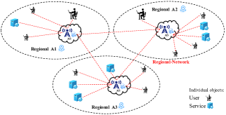
Figure 1. Objects typically exhibit network-state similarity within a region, especially if the regional network operates under the same autonomous system (AS).

To surmount these challenges, we introduce the regional network latent state learning (R2SL) approach, which adeptly harnesses regional network latent states to achieve precise QoS predictions. R2SL encompasses two regional network latent state varieties: city-network and AS-network. The city-network latent state derives insights from QoS data corresponding to objects from a specific city, while the AS-network latent state analyzes data from objects sharing an autonomous system. Initially, R2SL employs latent probability learning algorithms to frame regional network latent states, counteracting data sparsity effects in QoS prediction. Subsequently, an enhanced Huber loss function is deployed, modulating the linear loss component to tackle label imbalances. Lastly, a multi-scale convolution network extracts insights from the fused feature maps, which consolidate known features and regional network latent states, ensuring high-accuracy QoS predictions.

Our R2SL model offers two groundbreaking advances in QoS prediction. Firstly, we introduce the innovative concept of modeling regional latent network states as opposed to individual ones. This strategy capitalizes on regional QoS data to counter data sparsity, as illustrated in Fig. 1. Secondly, we present an optimized Huber loss function to elevate QoS prediction accuracy. Through meticulous analysis of QoS data label distributions, we fine-tuned the loss function to strike an optimal balance in the model’s learning capability for unbalanced labels, bolstering prediction performance.

In summary, this paper’s primary contributions are:

• Introduction of the R2SL approach, designed to harness regional network latent states, addressing data sparsity and cold start challenges in QoS prediction. By gleaning latent states from diverse regional networks, R2SL promises enhanced recommendation precision.

• Analysis of QoS data distribution characteristics, pinpointing label imbalance as a significant impediment. We introduce an enhanced Huber loss function, aiming to combat label imbalance and optimize prediction accuracy.

• Comprehensive experimentation evaluating the R2SL approach’s effectiveness on real-world QoS datasets. Experimental outcomes highlight R2SL’s superior performance over existing state-of-the-art QoS prediction methodologies. .

2. Related work

The existing body of work primarily hinges on two pivotal approaches for QoS prediction: Collaborative Filtering (CF) and Deep Learning (DL) methods.

2.1. CF-Based Approaches

Collaborative Filtering (CF) remains a predominant strategy for QoS prediction, where models draw insights from analogous objects to forecast the QoS (Lee et al., 2015; Chen et al., 2010; Zheng et al., 2010; Chen et al., 2017; Chowdhury et al., 2020). Broadly, CF methodologies bifurcate into: memory-based and model-based methods.

Memory-based methods lean on QoS metrics (e.g., response time, network throughput) or attributes (like distance) as differentiation indices among objects. The cornerstone of these techniques lies in computing similarities with the object in focus. Foundational CF strategies encompass user-based (e.g., UPCC)(Tan and He, 2017), service-based (e.g., IPCC)(Sarwar et al., 2001), and their hybrids, such as UIPCC (Ma et al., 2007). Notably, initiatives like GroupLens and Bellcore harnessed similar user reviews to prognosticate other users’ service sentiments (Konstan et al., 1997).

Conversely, model-based methods, especially matrix factorization (MF), have gained traction. These entail factorizing a request matrix into a product of two state matrices for QoS prediction. Illustratively, Luo et al. innovated a non-negative matrix decomposition for swift user-service matrix training (Luo et al., 2019). Others, like He et al., advanced hierarchical matrix factorization for clustered QoS matrices (He et al., 2014a). Also noteworthy is the Factorization Machine (FM), a pervasive method that discerns object feature interactions (Rendle, 2012). Variations of FM, such as those proffered by Tang et al., married CF with FM to optimize mobile service QoS predictions (Tang et al., 2019). However, a recurring challenge with these methods is their limited capacity to effectively harness available information.

Recent advancements are gravitating towards exploiting contextual object information (like IP or location) to amplify prediction accuracy. Yang et al.’s FM-based model, which utilized neighboring user information, is a case in point (Yang et al., 2021). Similarly, latent factor-focused QoS prediction methods are gaining popularity for their precision and scalability (Ryu et al., 2018; Feng and Huang, 2018; Koren et al., 2009). Luo et al.’s non-negative constrained latent factor learning model (NLF) exemplifies this shift (Luo et al., 2016).

2.2. Deep Learning-Based Approaches

The allure of Deep Learning (DL) for QoS prediction has surged recently, given its capacity to directly infer the intricate relationships between latent object features and QoS via deep neural networks. Our R2SL method aligns with this paradigm, aspiring for utmost predictive accuracy.

A plethora of research has been centered on harnessing extant information for optimizing prediction precision. For instance, Zhou et al.’s spatio-temporal model leveraged varying time segments to refine QoS prediction accuracy (Zhou et al., 2019). Wu et al. tapped into contextual information with their Deep Neural Model (DNM) for multi-metric QoS forecasting (Wu et al., 2021). Typically, DL necessitates an abundance of valid information to decipher the nonlinear relationships between features and anticipated labels. Novel endeavors, such as Xiong et al.’s deep hybrid model, further excavate additional information through a multi-layer perceptron (MLP)(Xiong et al., 2018). Others, like Wang et al., elevate predictive accuracy by discerning users’ and services’ varied latent states using an LDA-based pre-training mechanism(Wang et al., 2021). Predominantly, current DL-based QoS methodologies orbit around individual objects.

Our R2SL proposition draws inspiration from object-centric latent state learning approaches (Wang et al., 2021; Luo et al., 2018). The distinguishing facet of R2SL, in contrast to its peers, is its proficiency in discerning distinct network states per region. This granularity allows R2SL to learn latent states more effectively by capitalizing on a broader data swath.

3. Approach

The architecture of R2SL, depicted in Fig.2, comprises two primary modules: regional network latent state learning and QoS prediction.

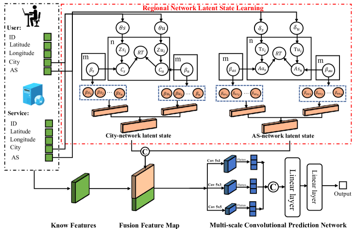
Figure 2. The R2SL architecture: regional network latent state learning (highlighted in orange) and the multi-scale convolutional prediction network. \small{c}⃝ indicates concatenation operations.

3.1. Regional Network Latent State Learning

3.1.1. Latent Regional State Variable

Define $L=(U,S,T,La_{s},Lo_{s},C_{s},As_{s},La_{u},Lo_{u},C_{u},As_{u})$, where $U$ and $S$ represent the user and service IDs, respectively. $C$ and $As$ denote city code and AS code, respectively. $T$ signifies the response time for user $U_{i}$ requesting $S_{i}$, constrained to $0s<T<20s$. Geographical and network metadata for services are represented by $La_{s},Lo_{s},C_{s},As_{s}$, and by $La_{u},Lo_{u},C_{u},As_{u}$ for users. The latent states set $B=\{b_{k}\}$ (where $1<k<m$) encompasses $m$ latent state variables needed by the services’ regional network and provided by the users’ regional network to conduct activities.

To determine the latent distribution of regional states, we employ a latent state learning algorithm. This approach aids in discerning the latent network states across diverse cities and AS. We initiate by defining two distributions, $\Theta_{s}$ and $\Theta_{u}$, symbolizing the AS-network state frequencies for users and services respectively. Analogously, for the city-network latent distribution, we have $\delta_{s}$ and $\delta_{u}$. Their mathematical representation is:

(1) $$\centering\Theta_{s},\Theta_{u},\delta_{u},\delta_{s}\sim Dirichlet(\alpha)\@add@centering$$

To refine these frequency variables, we introduce the Dirichlet Distribution characterized by parameter $\alpha$. $\alpha$ acts as the starting value of the potential state and, by default, is set to 5.

In essence, the prior distribution for the latent service-AS network state is given by $Q={\textstyle\prod^{m}}(\Theta_{s_{i}})^{\alpha-1}{\div}B(\alpha)$ and that for city-as states is $Q(\Theta_{u};\alpha)$. The procedure mirrors for $\delta_{u}$ and $\delta_{s}$.

3.1.2. Assignment Probability on Latent Regional State

The city network latent state for each user and service. Given $L$ and $B$, the probability of assigning latent city network state $b_{i}$ to user network $C_{u_{j}}$ is defined by ${\textstyle\sum_{n}^{j=i}}P(u_{j}\mid b_{i})=1$. Similarly, the probability of assigning latent city network states $b_{i}$ to service city $C_{s_{j}}$ is defined by $P(s_{j}\mid b_{i})$.

The AS network potential state for each user and service. The probability of assigning latent AS network states $b_{i}$ to user AS $As_{u_{j}}$ is $P_{a}(u_{j}\mid b_{i})$ and the probability of assigning latent AS network states $b_{i}$ to the service’ $As_{s_{j}}$ is $P_{a}(s_{j}\mid b_{i})$.

For presentation brevity, we denote $P(u_{j}\mid b_{i})$ by $\beta_{s\{i,j\}}$ and $P(u_{j}\mid b_{i})$ by $\beta_{u\{i,j\}}$. As the figure shows, for AS latent states, there are also $\beta_{as}$ and $\beta_{au}$.

The matrix $\beta_{s}=\beta_{s\{i,j\}}$ to denote the probability for assigning all $m$ latent city network states to all $C_{u_{i}}$ and $\beta_{u}=\beta_{u\{i,j\}}$ to denote the probability for assigning all $m$ latent service network states to all $C_{s_{i}}$.Similarly, we have $\beta_{au}$ for $AS_{u}$ and $\beta_{as}$ for $AS_{s}$.

3.1.3. Latent Parameters for RT

To model the nuanced influence of various regional state frequencies and assignments on QoS, we identify primary contributing factors that are the statistical properties of RT; these are termed as the Latent Parameters for RT.

Central to various QoS metrics is the step of sampling QoS value $T_{i}$ given the $i$-th QoS record $L$. In our discussion, $T_{i}$ represents the response time, although other metrics can be substituted. The observation value $T$ is susceptible to changes in the network states. Let $\Phi$ represent the probability density function based on the exponential distribution:

(2) $$\centering\Phi(T_{i},\lambda_{i,j,k})=\lambda_{i,j,k}e^{(-T_{i}*\lambda_{i,j,k})}\@add@centering$$

where

(3) $$\centering\lambda_{i,j,k}^{-1}=\begin{cases}Wu_{i}Ws_{j}&\text{ if }T_{i}<\eta\\ Wu_{i}Ws_{j}w&\text{ else }\end{cases}\@add@centering$$

Here, $i$ stands for the user’s city code (or AS code) and $j$ for the service’s city (or AS code) in the $i$-th record. Both $W_{u}$ and $W_{s}$ represent the complexity coefficients related to the QoS for users and services, respectively. They are initialized to a value of 10. The constant $\eta$ defaults to 5, while $w$, a trainable penalty coefficient, starts with an initial value of 50.

3.1.4. State Sampling

City network state sampling: City network state sampling: Our analysis follows this sampling methodology: the latent state originates from a state set of magnitude $m$, drawn in accordance with the frequency $\Theta_{u}$. Explicitly, the probability of latent states associated with $u_{i}$ is denoted as $Z_{u}$:

(4) $$\centering Z_{u}|\Theta_{u}\sim Discrete(\Theta_{u})\@add@centering$$

In a similar vein, the probability of the latent state associated with $s_{i}$ is expressed as $Z_{s}$:

(5) $$\centering Z_{s}|\Theta_{s}\sim Discrete(\Theta_{s})\@add@centering$$

AS network state sampling: Analogous computations yield:

(6) $$\centering T_{s}|\delta_{s}\sim Dirichlet(\delta_{s})\@add@centering$$

For the user’s AS-network $As_{u_{i}}$, we have:

(7) $$\centering T_{u}|\delta_{u}\sim Dirichlet(\delta_{u})\@add@centering$$

3.1.5. City/AS latent state Assignment

Then we assign the probability of the network state $Z_{u}$ to user’s city-network state and assigning service’s city-network $Z_{s}$ for each QoS record. To model the relation between the states $Z_{u}$ and $Z_{s}$ , we use the assignment probability $\beta_{s}$ as the parameter. The service’s city $C_{s_{j}}$ with network states $Z_{s\{i\}}$ is sampled from the following distribution:

(8) $$\centering C_{s}|Z_{s},\beta_{s}\sim Discrete(\beta_{s\{Z_{s}\}})\@add@centering$$

It means that the conditional probability of $C_{s}$ given the network state $z_{s_{i}}$ is exactly $\beta_{s\{Z_{s}\}}$.

Similarly, we introduce the user’s city-network latent state assignment probability $\beta_{u}$ to get the conditional probability

(9) $$\centering C_{u}|Z_{u},\beta_{u}\sim Discrete(\beta_{u\{Z_{u}\}})\@add@centering$$

$\beta_{s}$ and $\beta_{u}$ have size $n_{u}$ x $m$ and $n_{s}$ x $m$ respectively with m independent mixture ability components. $n_{u}$ and $n_{s}$ are the number of cities where the user is located and the number of cities where the service is located Similarly, for AS-Network, we have $A_{a_{u}},A_{a_{s}}$.

3.1.6. Quality of Service Sampling

The most important step is sampling response time $T_{i}$ given the i QoS record $L$. $T_{i}$ as the object of observation is affected by different factors of users and services. For each record, the conditional probability is used to represent its distribution:

(10) $$\centering T_{i}|Z_{u},Z_{s},A_{a_{u}},A_{a_{s}},W_{u},W_{s},w\sim\Phi(T_{i};\lambda_{i,j,k})\@add@centering$$

where f is the exponential distribution whose expectation is $\Phi$ as defined in eq 2.

3.1.7. Parameter estimation

City-network Latent State. The $\Lambda(\beta_{u},\beta_{s},\Theta_{u},\Theta_{s},w,W_{u},W_{s})$ is the set of parameters for city-network latent state. To complete the parameter estimation process, R2SL uses the maximum a posteriori (MAP) algorithm. The distribution $P(\Lambda|L)$ is learned by the true label $L$. The calculation process is as follows:

(11) $$\centering P(\Lambda|L)=\prod_{i=1}^{n}\sum_{j=1}^{m}\sum_{k=1}^{m}\Phi(T_{i};\lambda_{i,j,k})\tau_{i,j,k}\@add@centering$$

where

(12) $$\centering\tau_{i,j,k}=\beta_{u\left\{j,Cu_{i}\right\}}\beta_{s\left\{j,Cs_{i}\right\}}\Theta_{u\left\{j\right\}}\Theta_{s\left\{k\right\}}\frac{1}{B(M)}\prod_{i=1}^{m}(\Theta_{s\left\{i\right\}}\Theta_{s\left\{i\right\}})^{M-1}\@add@centering$$

Where $Cu_{i}$ and $Cs_{i}$ represent the city code or AS code of the i-th QoS recorded In order to estimate the parameter set $\left\{\Theta_{u},\Theta_{s},C_{u},C_{s}\right\}$, the expectation-maximization (EM) algorithm is used, At the same time, the set $\left\{W_{u},W_{s},w\right\}$ are estimated with the gradient descent (GD) algorithm.

AS-network Latent State. $\Gamma(\delta_{u},\delta_{s},\beta_{au},\beta_{as},w_{a},W_{u_{a}},W_{s_{a}})$ is a set of parameters for AS-network latent state. The specific calculation process is as follows:

(13) $$\centering P_{a}(\varphi|L)=\prod_{i=1}^{n}\sum_{j=1}^{m}\sum_{k=1}^{m}\Phi(T_{i};\lambda_{i,j,k})\tau_{i,j,k}\@add@centering$$

where

(14) $$\centering\tau_{i,j,k}=\beta_{au\left\{j,As_{u_{i}}\right\}}\beta_{as\left\{j,As_{s_{i}}\right\}}\delta_{u\left\{j\right\}}\delta_{s\left\{k\right\}}\frac{1}{B(M)}\prod_{i=1}^{m}(\delta_{s\left\{i\right\}}\delta_{s\left\{i\right\}})^{M-1}\@add@centering$$

Algorithm 1 Network Latent State Learning Algorithm

0:  $L$

0:  ($\beta_{au},\beta_{as}$, $\beta_{u},\beta_{s}$)

  for $H=1$ to $2$ do

     while $\tau^{t+1}/\tau^{t}>\gamma$ do

        for $i=1$ to $n$ do

           for $j=1$ to $m$ do

              for $k=1$ to $m$ do

                 $G_{i,j,k}^{t}=\tau_{i,j,k}\Phi(T_{i};\lambda_{i,j,k})$

              end for

           end for

        end for

        for $i=1$ to $m$ do

           $\Theta_{u}^{t+1}=\frac{(m-1)n+\sum_{i^{{}^{\prime}}=1}^{n}\sum_{k=1}^{m}G_{i^{{}^{\prime}},i,k}^{t}}{n(m(m-1)+1)}$

           $\Theta_{s}^{t+1}=\frac{(m-1)n+\sum_{i^{{}^{\prime}}=1}^{n}\sum_{j=1}^{m}G_{i^{{}^{\prime}},j,i}^{t}}{n(m(m-1)+1)}$

           if H==1 then

              for $q=1$ to $n_{cu}$ do

                 $\beta_{u\left\{i,q\right\}}^{t+1}=\sum_{i^{{}^{\prime}}=1}^{n}\sum_{k=1}^{m}G_{i^{{}^{\prime}},i,k}^{t}I(C_{u_{i}}=q)$

              end for

              for $p=1$ to $n_{cs}$ do

                 $\beta_{s\left\{i,q\right\}}^{t+1}=\sum_{i^{{}^{\prime}}=1}^{n}\sum_{j=1}^{m}G_{i^{{}^{\prime}},j,i}^{t}I(C_{s_{i}}=p)$

              end for

           end if

           if H==2 then

              for $q=1$ to $n_{au}$ do

                 $\beta_{au\left\{i,q\right\}}^{t+1}=\sum_{i^{{}^{\prime}}=1}^{n}\sum_{k=1}^{m}G_{i^{{}^{\prime}},i,k}^{t}I(As_{u_{i}}=q)$

              end for

              for $p=1$ to $n_{as}$ do

                 $\beta_{as\left\{i,q\right\}}^{t+1}=\sum_{i^{{}^{\prime}}=1}^{n}\sum_{j=1}^{m}G_{i^{{}^{\prime}},j,i}^{t}I(As_{s_{i}}=p)$

              end for

           end if

        end for

        if H==1 then

           for $q=1$ to $n_{cu}$ do

              $Wu_{i}^{t+1}=Wu_{i}^{t}+\varrho*\frac{\partial P(\Gamma|L)^{t}}{\partial Wu_{i}^{t}}$

           end for

           for $q=1$ to $n_{cs}$ do

              $Ws_{i}^{t+1}=Ws_{i}^{t}+\varrho*\frac{\partial P(\Gamma|L)^{t}}{\partial Ws_{i}^{t}}$

           end for

           $t=t+1$

           $w^{t+1}=w^{t}+\varrho*\frac{\partial P(\Gamma|L)^{t}}{\partial w^{t}}$

           $\tau^{t+1}=P(\Gamma|L)$

        end if

        if H==2 then

           for $q=1$ to $n_{cu}$ do

              $Wu_{i}^{t+1}=Wu_{i}^{t}+\varrho*\frac{\partial P(\Gamma|L)^{t}}{\partial Wu_{i}^{t}}$

           end for

           for $q=1$ to $n_{cs}$ do

              $Ws_{a_{i}}^{t+1}=Ws_{a_{i}}^{t}+\varrho*\frac{\partial P(\Gamma|L)^{t}}{\partial Ws_{a_{i}}^{t}}$

           end for

           $t=t+1$

           $w_{a}^{t+1}=w^{t}+\varrho*\frac{\partial P(\Gamma|L)^{t}}{\partial w_{a}^{t}}$

           $\tau^{t+1}=P(\Gamma|L)$

        end if

     end while

  end forreturn ($\beta_{au},\beta_{as}$,$\beta_{u},\beta_{s}$)

In Algorithm 1, we update the probability distribution of latent network state:

(15) $$F_{i,j,k}^{t} =P(Cu_{i},t_{k}|Cu_{i},Cs_{i},t_{i},\Gamma)$$

$$=\tau_{i,j,k}\Phi(T_{ij};\lambda_{i,j,k})$$

We use maximizing the condition expectation to update parameters $\Gamma$.

(16) $$\Theta_{s}^{t+1},\Theta_{u}^{t+1},\beta_{s}^{t+1},\beta_{u}^{t+1}=maxT(\Gamma|\Gamma^{t})$$

(17) $$T(\Gamma|\Gamma^{t}) =\sum_{i=1}^{n}\sum_{j=1}^{m}\sum_{k=1}^{m}log(P(\Gamma|Q))F_{i,j,k}^{t}$$

$$=\sum_{i=1}^{n}\sum_{j=1}^{m}\sum_{k=1}^{m}log(\tau_{i,j,k}\Phi(T_{ij};\lambda_{i,j,k}))F_{i,j,k}^{t}$$

Then we have:

(18) $$\Theta_{s}^{t+1} =arg_{\Theta_{u}}maxT(\Gamma|\Gamma^{t})$$

$$=\frac{\sum_{i^{{}^{\prime}}=1}^{n}\sum_{k=1}^{m}F_{i^{{}^{\prime}},i,k}^{t}+(m-1)n}{n(m(m-1)+1)}$$

Similarly, by the derivative calculation, we update $\Theta_{u}^{t+1}$. Next, we consider $\beta_{u}$, with the constraint ${\textstyle\sum_{j}^{n_{u}}}\beta_{u_{\{}j,q\}}=1$. We update $\beta_{u}$ by solving:

(19) $$\beta_{u_{j,p}}^{t+1}= arg_{\beta_{u}}maxT(\Gamma|\Gamma^{t})$$

$$=\sum_{i=1}^{n}\sum_{k=1}^{m}F_{i,j,k}^{t}I(C_{u_{i}}=q)$$

Similarly, for $\beta_{s}$:

(20) $$\beta_{s_{k,q}}^{t+1}= arg_{\beta_{s}}maxT(\Gamma|\Lambda^{t})$$

$$=\sum_{i=1}^{n}\sum_{j=1}^{m}F_{i,j,k}^{t}I(C_{s_{i}}=p)$$

where $I(C_{u_{i}}=q)$ means that the final value of the function is 1 when user’s city code is equal to q and 0 otherwise; $I(C_{s_{i}}=q)$ means that the value of the function is 1 when service’s city code is equal to p and 0 otherwise. Finally, we obtain the user city-network latent state distribution $\beta_{u}$ and the service city-network latent state distribution $\beta_{s}$ through Algorithm 1. For AS-network latent state learning, we replace the city information in Algorithm 1 with the AS information and obtain $\beta_{au}$, $\beta_{as}$ by the same calculation process.

3.2. QoS Prediction

Feature Embedding. For deep neural networks to effectively learn prominent features, we input identifiers such as the user ID, user’s city code, AS code, service ID, service’s city code, and AS code into the embedding layer provided by TensorFlow. Conceptually, the embedding layer can be regarded as a linear layer where the bias is 0 (Lee et al., 2015). Using this approach, the distinguishable features (i.e., ID, city code, and AS code) are mapped into distinct vectors.

Known Feature. We create the integrated known feature map by embedding the known features as discussed in L(Sec.3.1.1). The dimensions of this known feature map are defined as:

(21) $$KF=\begin{bmatrix}I^{k}_{u},La^{k}_{u},Lo^{k}_{u},U^{k}_{u},As^{k}_{u}\\ I^{k}_{s},La^{k}_{s},Lo^{k}_{s},U^{k}_{s},As^{k}_{s}\end{bmatrix}$$

Regional Network Latent States Feature. To construct the latent states map, we employ city-network latent features combined with AS-network latent states. By default in the R2SL framework, the model extracts $m$ latent states for each region, with $m$ defaulting to 5. The impacts of varying $m$ and related parameters are elaborated upon in Sec.5.4. Thus, the dimensions of the latent states map are $4\times m$:

(22) $$LF=\left[\begin{array}[]{cccc}\beta_{u,1}^{k},&\beta_{u,2}^{k},&\cdots&\beta_{u,m}^{k}\\ \beta_{s,1}^{k},&\beta_{s,2}^{k},&\cdots&\beta_{s,m}^{k}\\ \beta_{au,1}^{k},&\beta_{au,2}^{k},&\cdots&\beta_{au,m}^{k}\\ \beta_{as,1}^{k},&\beta_{as,2}^{k},&\cdots&\beta_{as,m}^{k}\end{array}\right]$$

Fuse Feature Map. By integrating latent state features with known features, we derive the fused feature map. The resulting dimensions of this map are $6\times m$.

(23) $$O=\begin{bmatrix}KF\\ LF\end{bmatrix}$$

Adjustable Multi-scale Convolutional Network. Our approach extracts features via a Adjustable multi-scale convolutional network, which enables extraction from varying perspectives of the fused features. The kernel size will change adaptively according to the number of latent network state you set.

(24) $$X_{i}=f(O;\mathbf{w}_{i}),i=1,2,3.$$

Here, $\mathbf{w}_{i}$ denotes a 2-dimensional convolutional kernel. The kernels for the three convolutional networks are defined as mx1, mx3, and mx5, respectively.

Subsequently, we integrate the fusion features with sampling features and channel them through a convolutional layer. The final QoS prediction is achieved via a fully connected network:

(25) $$x=F(X_{1})\oplus F(X_{2})\oplus F(X_{3}).$$

(26) $$\hat{y}=f^{[2^{v},2^{v-1},2^{v-2},1]}(x;\mathbf{W}_{x}).$$

where $\Phi$ is represents the mergence operation. $F$ is represents the flatten operation by Flatten of Keras. $f^{[2^{v},2^{v-1},2^{v-2},1]}$ denotes the fully connected layer, $V$ is the count of neurons in this layer, and $\hat{y}$ the prediction value.

3.3. E-Huber Loss Function

For QoS prediction, the Mean Absolute Error (MAE) loss function is prevalently employed. The MAE loss function directs the model to concentrate on normal values, while being minimally affected by outliers. Some research has adopted the Huber loss to enhance the model’s attention to outliers. Broadly speaking, the Huber loss demonstrates higher sensitivity to outliers compared to the MAE loss and exhibits greater robustness than the Root Mean Square Error (RMSE) loss.

In our exploration of QoS data distribution detailed in Sec. 4, we discerned that the linear component of the Huber loss remains significantly large, causing the model to still not adequately focus on outliers. R2SL addresses this by re-weighting the linear component of the Huber loss function in accordance with the intrinsic characteristics of the QoS data distribution. The novel loss function, termed the E-Huber loss, is adept at capturing the extended tail of QoS data.

The E-Huber loss function between $y$ and $\hat{y}$ is given by:

(27) $$E-Huber_{loss}(y,\hat{y})=\left\{\begin{matrix}\frac{1}{2}(y-\hat{y})^{2}&if\ |y-\hat{y}|_{abs}<\varsigma,\\ \psi(\varsigma|y-\hat{y}|_{abs}-\frac{1}{2}\varsigma^{2})&otherwise.\end{matrix}\right.$$

Here, $y$ represents the actual label, $\hat{y}$ is the predicted value, and $\varsigma$ is the Huber loss hyperparameter, defaulting to 0.5.

Motivation and Improvement. The Huber loss function boasts enhanced resilience to outliers as opposed to both MAE and MSE loss functions. As per its definition, Huber loss equates to RMSE when the error is smaller than $\varsigma$. Conversely, for errors surpassing $\varsigma$, the loss corresponds to MAE. Nonetheless, extreme values in QoS data render the Huber loss suboptimal for directing model training. For instance, a long-tail label (e.g., 20s) might yield a linear loss exceeding 15, while a standard label (e.g., 1.5s) might result in an MSE loss approaching 0.25. This pronounced disparity causes the model to be disproportionately swayed by long-tail labels. To mitigate this, we introduced a weighting factor to the linear loss segment. Manipulating this coefficient’s value permits the model to more proficiently characterize the long-tail labels. Therefore, diverging from the traditional Huber loss function, $\psi$ acts as the weight for the linear loss component, and is set at 0.05 in this paper.

4. STUDY SETUP

Table 1. Division of all designed dataset cases.

No.	Density	Train:Test:Valid	Train	Test	Validation
D1.1	0.02	2%:78%:20%	37,375	1,310,535	369,638
D1.2	0.04	4%:76%:20%	74,969	1,572,292	369,638
D1.3	0.06	6%:74% :20%	112,016	1,206,517	369,638
D1.4	0.08	8%:72% :20%	150,071	1,172,461	369,638
D1.5	0.10	10%:70% :20%	186,059	1,140,269	369,638

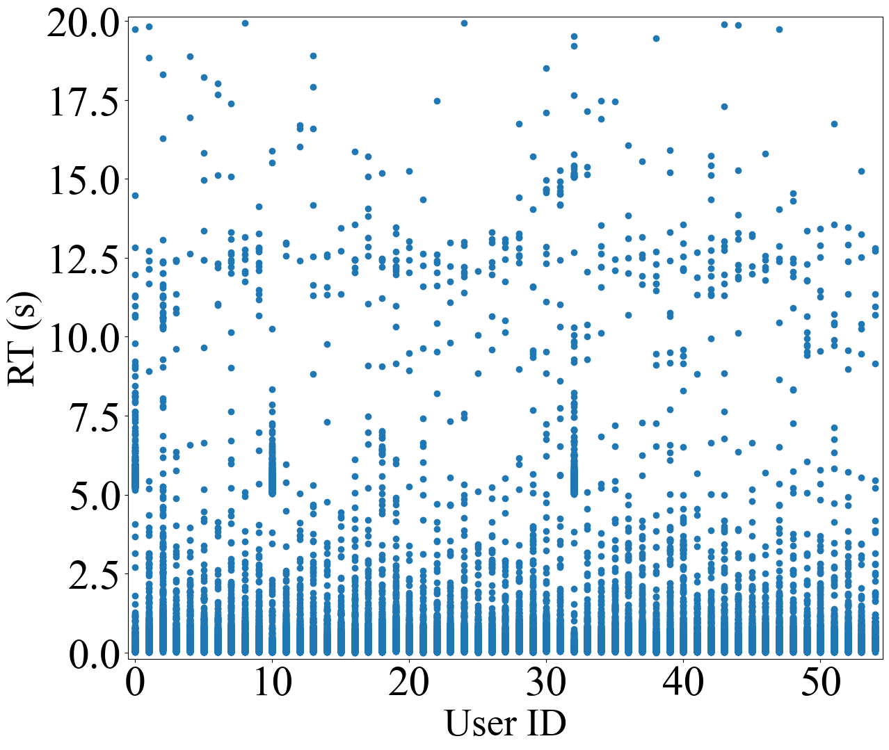
(a) QoS data distribution

(b) Data distribution of five user

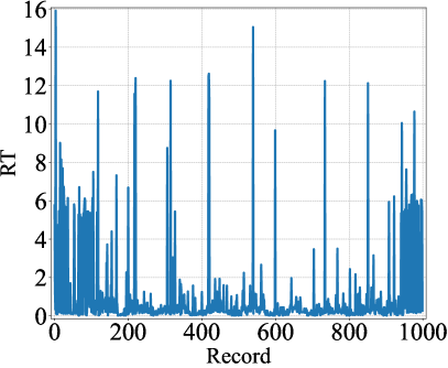
(c) A user accesses service 0-1000

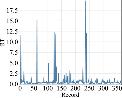
(d) User 0-350 accesses the service A

Figure 3. QoS distribution of datasets

4.1. Datasets

We conducted validation experiments on publicly available benchmark datasets. The QoS dataset, termed WS-Dream, contains service data harvested from real-world web systems as detailed by  (Zheng et al., 2010). As depicted in Tab. 2, this dataset, concerning response time, encompasses over 1,900,000 web service request records.

Of significance, the dataset utilized in this research is derived from the most recent investigation by  (Ye et al., 2021), which refines the WS-Dream data by removing outliers. Adhering to their methodology, we employed the iForest (isolation forest) approach for outlier detection, maintaining the detection parameters consistent with  (Ye et al., 2021). The threshold for outlier scoring is in alignment with  (Ye et al., 2021), set at 0.1.

For a comprehensive analysis, the dataset was segmented into five divisions, as presented in Tab. 3. These divisions were made to emulate data sparsity scenarios in real-world production environments and to ensure robust comparative experimentation. The data distribution for the WS-Dream dataset is depicted in Fig.3. A conspicuous observation from this figure is the pronounced label imbalance within the QoS dataset.

Table 2. Experimental Results

Method	D1.1		D1.2		D1.3		D1.4		D1.5
	MAE	RMSE	MAE	RMSE	MAE	RMSE	MAE	RMSE	MAE	RMSE
UPCC	0.542	1.022	0.466	0.820	0.428	0.787	0.389	0.754	0.555	1.317
IPCC	0.520	1.121	0.473	0.900	0.437	0.838	0.427	0.829	0.596	1.342
UIPCC	0.506	1.075	0.462	0.878	0.427	0.820	0.415	0.808	0.584	1.329
D2E-LF	0.653	1.638	0.633	1.577	0.607	1.564	0.600	1.563	0.590	1.556
HMF	0.349	0.674	0.277	0.579	0.261	0.551	0.256	0.532	0.256	0.526
LDCF	0.349	0.987	0.279	0.794	0.247	0.751	0.240	0.711	0.213	0.692
CMF	0.327	0.657	0.294	0.605	0.250	0.536	0.231	0.496	0.205	0.461
NCRL	0.312	0.953	0.252	0.772	0.221	0.722	0.201	0.662	0.182	0.660
HSA-Net	0.182	0.558	0.159	0.495	0.128	0.470	0.128	0.448	0.126	0.442
R2SL	0.151	0.440	0.124	0.393	0.114	0.359	0.109	0.342	0.104	0.335

Fig.3(a) delineates the QoS records of 50 users, chosen randomly from the WS-Dream dataset, constituting 277,615 QoS record values. The data exhibits a mean of 0.770 and a variance of 3.454. Delving deeper, 95.10% of the labels register values below 5, while the remaining 4.90% exceed this value. Fig.3(b) catalogues the request records of 5825 services sourced from five users. It’s evident that the response time for a preponderant number of requests is under $5s$.

Fig.3(c) showcases the response time for user A when accessing services ranging from 0 to 1000. Predominantly, user A achieves access within $4s$, yet there are certain services where the response time overshoots $10s$. Conversely, Fig.3(d) demonstrates that for Service S, while the majority of user response times hover below $2.5s$, some instances report times exceeding $10s$. This underscores the influence of both user and service network states on the resultant quality of web requests.

4.2. Evaluation Metrics

The accuracy of the QoS prediction is an important criterion for evaluating the performance of the model. Two metrics (i.e. MAE and RMSE) are commonly used to measure accuracy in most QoS prediction studies (Ye et al., 2021). The mean absolute error function (MAE) is defined as follows:

(28) $$\centering MAE=\frac{\left(\sum_{i,j}\left|r_{i,j}-\hat{r}_{i,j}\right|_{abs}\right)}{N}\@add@centering$$

where $r_{i,j}$ is the real QoS value (e.g., RT or TP) and $\hat{r}_{i,j}$ is the predicted value from predictive models. The root mean squared error (RMSE) is defined as follows

(29) $$\centering RMSE=\sqrt{\tfrac{\left(\sum_{i,j}(r_{i,j}-\hat{r}_{i,j})^{2}\right)}{N}}\@add@centering$$

where N is the count of records. For either the MAE indicator or the RMSE indicator, a lower value means higher predictive accuracy.

4.3. Baseline Methods

We compare our R2SL approach with the following these methods:IPCC (CarlKadie, 1998),UPCC (Sarwar et al., 2001), UIPCC (Zheng et al., 2010), HMF (He et al., 2014b), LDCF (Zhang et al., 2019), CMF (Ye et al., 2021), HSA-Net (Wang et al., 2021),D2E-LF(Wu et al., 2022),NCRL (Zou et al., 2022).

In all experimental results, each method will be run five times and the results will be averaged for a fair comparison and other settings remain the same as CMF (Ye et al., 2021). We benchmark R2SL against six baselines, encompassing both traditional CF-based algorithms and cutting-edge deep learning approaches. Specifically, LDCF represents the latest in QoS prediction, leveraging collaborative filtering of location data. For our experiments, LDCF is configured as described in its source paper. CMF, another contemporary method focusing on outlier-based QoS prediction, provided the experimental dataset. It, too, is set with its default parameters as specified in its original publication. HSA-Net, a state-of-the-art latent state-based QoS prediction model, is trained using parameters initially proposed to discern user and service latent states.

4.4. Research Questions

Through rigorous experiments, this section intends to unveil the relative merits of our model, while elucidating the underlying reasons for its exemplary performance. We are particularly focused on addressing the ensuing research queries:

1. How does R2SL approach compare to the current state of the art baselines in terms of QoS prediction?

2. What is the effect of different latent region states on the prediction performance?

3. What is the impact of this E-huber loss on the prediction performance?

5. EXPERIMENTS

In this section, we conduct thorough experiments to evaluate the prediction performance of R2SL against state-of-the-art baselines. We also delve into the influence of various modules and parameters on R2SL’s performance through ablation studies.

5.1. RQ1: Prediction Performance Comparison

As shown in Table 4, in machine learning-based models, most of the collaborative prediction algorithm models exhibit similar predictive capabilities. When considering CMF, it outperforms HMF in terms of RMSE and MAE metrics, owing to CMF’s ability to concurrently utilize contextual data rather than relying solely on QoS-based collaborative filtering. D2E-LF is the latest collaborative filtering algorithm with impressive training and prediction speeds, but it is limited by the extreme sparsity of the data, resulting in lower predictive accuracy on this dataset.

NCRL is the latest QoS prediction method based on deep learning, which maximizes the use of known features to achieve high prediction accuracy. CMF, innovating with its outlier optimization approach, and HSA-Net, capitalizing on deep learning with latent states, both present impressive results. CMF not only excels in predictive performance among non-deep models but also boasts a streamlined computational process. When juxtaposed with HSA-Net, the top performer among our baselines, R2SL achieves reductions of 14.17%, 17.03%, 11.32%, 11.56%, and 14.86% in MAE, and 13.06%, 11.76%, 9.62%, 20.91%, and 18.86% in RMSE. On the QoS dataset, R2SL’s proficiency in discerning high-dimensional latent distributions is evident, outpacing HSA-Net, which employs a latent state learning approach for accuracy enhancement.

5.2. RQ2: The Effect of Network Latent States

To discern the influence of network latent states on prediction performance, we instituted four comparative experiments:

a) R2SL: Employs the default state fusion map encompassing all known features and latent states.

b) R2SL w/o C: Excludes city-network latent states from the R2SL’s feature fusion map.

c) R2SL w/o A: Omits AS-network latent states from the R2SL’s feature fusion map.

d) R2SL w/o H: Removes all latent states from the R2SL’s feature fusion map.

As illustrated in Fig. 4, R2SL demonstrates a prediction performance that outstrips the rest. Specifically, experiments a), b), and c) exhibit analogous results. Experiment d), by virtue of including all the network latent states found in a), b), and c), can harness a richer set of network state data for refined prediction accuracy. Additionally, d) proves especially potent in scenarios characterized by sparser training data. Contrastingly, a) which relies solely on known data points, underperforms in both MAE and RMSE metrics when set against its latent state-utilizing counterparts. These findings underscore the pivotal role latent states play as bolstering features for QoS prediction.

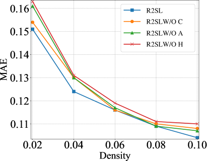
(a) MAE

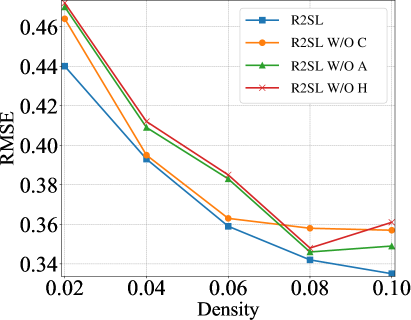
(b) RMSE

Figure 4. The results for different regional network states

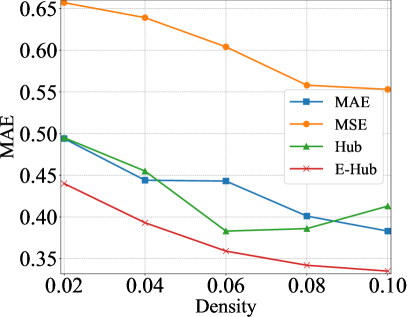
(a) MAE

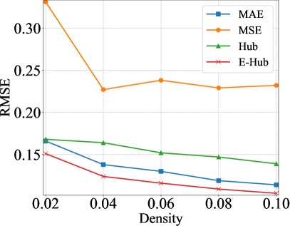
(b) RMSE

Figure 5. The results of R2SL with different loss function

5.3. RQ3: Loss Function for Data Imbalance

To ascertain the efficacy of our introduced E-Huber loss function, we employed diverse loss functions on the standard R2SL network with the D1.1 dataset. Throughout the evaluation, all parameters remained consistent, defaulting to their standard values. The hyperparameter $\delta$ for the Huber loss was calibrated identically to that of the E-Huber loss, set at $\delta=0.5$. We conducted experiments using MAE, MSE, Huber loss and E-Huber loss, respectively.

The MAE and MSE loss functions were derived from the standard formulations provided in TensorFlow.

Employing the D1.1 dataset, we gauged the merit of the proposed E-Huber loss function vis-à-vis the standard R2SL network. Our findings indicated that the MSE loss trailed in effectiveness. Both MAE and Huber loss exhibited akin trajectories. E-Huber loss excelled, a consequence of the dataset predominantly featuring brief response durations, interspersed with rare, extended exceptions. While the Huber loss manifested a diminished sensitivity to outliers compared to the MSE loss and showcased greater resilience than the MAE loss, the E-Huber loss adeptly amalgamated the strengths of both, leading in both MAE and RMSE performance metrics.

6. CONCLUSION

This paper has elucidated challenges inherent in QoS prediction, pinpointing two predominant issues: data sparsity and label imbalance. Specifically, the dearth of user data has curtailed the efficacy of prior latent factor-based prediction techniques. Concurrently, label imbalance can compromise the precision of deep models when discerning the interplay between features and QoS. In response to these impediments, we postulate a region-centric network similarity hypothesis and put forth the Regional Network Latent State Learning Network (R2SL) model. And it deploys an enhanced loss function to redress label imbalance. Our empirical analyses attest to R2SL’s superior performance over contemporary QoS prediction methods, registering an average decrement in MAE error of 13.78% when benchmarked against prevailing datasets. Looking ahead, we intend to devise even more potent prediction algorithms to bolster accuracy and accommodate expansive datasets. We are also poised to weave in auxiliary contextual data to probe the influence of similarity on service caliber across geographical locales.

- (1)
- CarlKadie (1998) JohnS Breese DavidHeckerman CarlKadie. 1998. Empirical analysis of predictive algorithms for collaborative filtering. Microsoft Research Microsoft Corporation One Microsoft Way Redmond, WA 98052 (1998).
- Chattopadhyay et al. (2022) Soumi Chattopadhyay, Richik Chanda, Suraj Kumar, and Chandranath Adak. 2022. OffDQ: An Offline Deep Learning Framework for QoS Prediction. In Proceedings of the ACM Web Conference 2022. 1987–1996.
- Chen et al. (2010) Xi Chen, Xudong Liu, Zicheng Huang, and Hailong Sun. 2010. Regionknn: A scalable hybrid collaborative filtering algorithm for personalized web service recommendation. In 2010 IEEE international conference on web services. IEEE, 9–16.
- Chen et al. (2017) Zhen Chen, Limin Shen, Feng Li, and Dianlong You. 2017. Your neighbors alleviate cold-start: On geographical neighborhood influence to collaborative web service QoS prediction. Knowledge-Based Systems 138 (2017), 188–201.
- Chowdhury et al. (2020) Ranjana Roy Chowdhury, Soumi Chattopadhyay, and Chandranath Adak. 2020. Cahphf: context-aware hierarchical QoS prediction with hybrid filtering. IEEE Transactions on Services Computing (2020).
- Feng and Huang (2018) Yu Feng and Biqing Huang. 2018. Cloud manufacturing service QoS prediction based on neighbourhood enhanced matrix factorization. Journal of Intelligent Manufacturing (2018), 1–12.
- He et al. (2014a) Pinjia He, Jieming Zhu, Zibin Zheng, Jianlong Xu, and Michael R. Lyu. 2014a. Location-Based Hierarchical Matrix Factorization for Web Service Recommendation. In 2014 IEEE International Conference on Web Services. 297–304. https://doi.org/10.1109/ICWS.2014.51
- He et al. (2014b) Pinjia He, Jieming Zhu, Zibin Zheng, Jianlong Xu, and Michael R Lyu. 2014b. Location-based hierarchical matrix factorization for web service recommendation. In 2014 IEEE international conference on web services. IEEE, 297–304.
- Hussain et al. (2022) Walayat Hussain, José M Merigó, Muhammad Raheel Raza, and Honghao Gao. 2022. A new QoS prediction model using hybrid IOWA-ANFIS with fuzzy C-means, subtractive clustering and grid partitioning. Information Sciences 584 (2022), 280–300.
- Konstan et al. (1997) Joseph A Konstan, Bradley N Miller, David Maltz, Jonathan L Herlocker, Lee R Gordon, and John Riedl. 1997. Grouplens: Applying collaborative filtering to usenet news. Commun. ACM 40, 3 (1997), 77–87.
- Koren et al. (2009) Yehuda Koren, Robert Bell, and Chris Volinsky. 2009. Matrix factorization techniques for recommender systems. Computer 42, 8 (2009), 30–37.
- Lee et al. (2015) Kwangkyu Lee, Jinhee Park, and Jongmoon Baik. 2015. Location-based web service QoS prediction via preference propagation for improving cold start problem. In 2015 IEEE International Conference on Web Services. IEEE, 177–184.
- Liu et al. (2015) Jianxun Liu, Mingdong Tang, Zibin Zheng, Xiaoqing Liu, and Saixia Lyu. 2015. Location-aware and personalized collaborative filtering for web service recommendation. IEEE Transactions on Services Computing 9, 5 (2015), 686–699.
- Luo et al. (2019) Xin Luo, MengChu Zhou, Zidong Wang, Yunni Xia, and Qingsheng Zhu. 2019. An Effective Scheme for QoS Estimation via Alternating Direction Method-Based Matrix Factorization. IEEE Transactions on Services Computing 12, 4 (2019), 503–518. https://doi.org/10.1109/TSC.2016.2597829
- Luo et al. (2016) Xin Luo, MengChu Zhou, Yunni Xia, Qingsheng Zhu, Ahmed Chiheb Ammari, and Ahmed Alabdulwahab. 2016. Generating highly accurate predictions for missing QoS data via aggregating nonnegative latent factor models. IEEE transactions on neural networks and learning systems 27, 3 (2016), 524–537.
- Luo et al. (2018) Zhiling Luo, Ling Liu, Jianwei Yin, Ying Li, and Zhaohui Wu. 2018. Latent Ability Model: A Generative Probabilistic Learning Framework for Workforce Analytics. IEEE Transactions on Knowledge and Data Engineering 31, 5 (2018), 923–937.
- Ma et al. (2007) Hao Ma, Irwin King, and Michael R Lyu. 2007. Effective missing data prediction for collaborative filtering. In Proceedings of the 30th annual international ACM SIGIR conference on Research and development in information retrieval. 39–46.
- Muslim et al. (2022) Hafiz Syed Muhammad Muslim, Saddaf Rubab, Malik M Khan, Naima Iltaf, Ali Kashif Bashir, and Kashif Javed. 2022. S-RAP: relevance-aware QoS prediction in web-services and user contexts. Knowledge and Information Systems 64, 7 (2022), 1997–2022.
- Park et al. (2021) Jinwoo Park, Byungkwon Choi, Chunghan Lee, and Dongsu Han. 2021. GRAF: a graph neural network based proactive resource allocation framework for SLO-oriented microservices. In Proceedings of the 17th International Conference on emerging Networking EXperiments and Technologies. 154–167.
- Rendle (2012) Steffen Rendle. 2012. Factorization Machines with LibFM. ACM Trans. Intell. Syst. Technol. 3, 3, Article 57 (may 2012), 22 pages.
- Ryu et al. (2018) Duksan Ryu, Kwangkyu Lee, and Jongmoon Baik. 2018. Location-based web service QoS prediction via preference propagation to address cold start problem. IEEE Transactions on Services Computing (2018).
- Sarwar et al. (2001) Badrul Sarwar, George Karypis, Joseph Konstan, and John Riedl. 2001. Item-based collaborative filtering recommendation algorithms. In Proceedings of the 10th international conference on World Wide Web. 285–295.
- Tan and He (2017) Zhenhua Tan and Liangliang He. 2017. An efficient similarity measure for user-based collaborative filtering recommender systems inspired by the physical resonance principle. IEEE Access 5 (2017), 27211–27228.
- Tang et al. (2019) M. Tang, W. Liang, Y. Yang, and J. Xie. 2019. A Factorization Machine-based QoS Prediction Approach for Mobile Service Selection. IEEE Access (2019), 1–1.
- Wang et al. (2021) Ziliang Wang, Xiaohong Zhang, Meng Yan, Ling Xu, and Dan Yang. 2021. HSA-Net: Hidden-State-Aware Networks for High-Precision QoS Prediction. IEEE Transactions on Parallel and Distributed Systems 33, 6 (2021), 1421–1435.
- Wu et al. (2022) Di Wu, Peng Zhang, Yi He, and Xin Luo. 2022. A double-space and double-norm ensembled latent factor model for highly accurate web service QoS prediction. IEEE Transactions on Services Computing 16, 2 (2022), 802–814.
- Wu et al. (2021) Hao Wu, Zhengxin Zhang, Jiacheng Luo, Kun Yue, and Ching-Hsien Hsu. 2021. Multiple Attributes QoS Prediction via Deep Neural Model with Contexts*. IEEE Transactions on Services Computing 14, 4 (2021), 1084–1096. https://doi.org/10.1109/TSC.2018.2859986
- Xiong et al. (2018) Ruibin Xiong, Jian Wang, Neng Zhang, and Yutao Ma. 2018. Deep hybrid collaborative filtering for web service recommendation. Expert systems with Applications 110 (2018), 191–205.
- Yang et al. (2021) Yatao Yang, Zibin Zheng, Xiangdong Niu, Mingdong Tang, Yutong Lu, and Xiangke Liao. 2021. A Location-Based Factorization Machine Model for Web Service QoS Prediction. IEEE Transactions on Services Computing 14, 5 (2021), 1264–1277. https://doi.org/10.1109/TSC.2018.2876532
- Ye et al. (2021) Fanghua Ye, Zhiwei Lin, Chuan Chen, Zibin Zheng, and Hong Huang. 2021. Outlier-Resilient Web Service QoS Prediction. In Proceedings of the Web Conference 2021. 3099–3110.
- Zhang et al. (2019) Yiwen Zhang, Chunhui Yin, Qilin Wu, Qiang He, and Haibin Zhu. 2019. Location-aware deep collaborative filtering for service recommendation. IEEE Transactions on Systems, Man, and Cybernetics: Systems (2019).
- Zheng et al. (2010) Zibin Zheng, Hao Ma, Michael R Lyu, and Irwin King. 2010. Qos-aware web service recommendation by collaborative filtering. IEEE Transactions on services computing 4, 2 (2010), 140–152.
- Zheng et al. (2020a) Zibin Zheng, Li Xiaoli, Mingdong Tang, Fenfang Xie, and Michael R Lyu. 2020a. Web service QoS prediction via collaborative filtering: A survey. IEEE Transactions on Services Computing (2020).
- Zheng et al. (2020b) Zibin Zheng, Li Xiaoli, Mingdong Tang, Fenfang Xie, and Michael R Lyu. 2020b. Web service QoS prediction via collaborative filtering: A survey. IEEE Transactions on Services Computing (2020).
- Zhou et al. (2019) Qimin Zhou, Hao Wu, Kun Yue, and Ching-Hsien Hsu. 2019. Spatio-temporal context-aware collaborative QoS prediction. Future Generation Computer Systems 100 (2019), 46–57.
- Zou et al. (2022) Guobing Zou, Shaogang Wu, Shengxiang Hu, Chenhong Cao, Yanglan Gan, Bofeng Zhang, and Yixin Chen. 2022. NCRL: Neighborhood-Based Collaborative Residual Learning for Adaptive QoS Prediction. IEEE Transactions on Services Computing (2022).