A Learning-Based Framework for Safe Human-Robot Collaboration with Multiple Backup Control Barrier Functions

Abstract

Ensuring robot safety in complex environments is a difficult task due to actuation limits, such as torque bounds. This paper presents a safety-critical control framework that leverages learning-based switching between multiple backup controllers to formally guarantee safety under bounded control inputs while satisfying driver intention. By leveraging backup controllers designed to uphold safety and input constraints, backup control barrier functions (BCBFs) construct implicitly defined control invariance sets via a feasible quadratic program (QP). However, BCBF performance largely depends on the design and conservativeness of the chosen backup controller, especially in our setting of human-driven vehicles in complex, e.g, off-road, conditions. While conservativeness can be reduced by using multiple backup controllers, determining when to switch is an open problem. Consequently, we develop a broadcast scheme that estimates driver intention and integrates BCBFs with multiple backup strategies for human-robot interaction. An LSTM classifier uses data inputs from the robot, human, and safety algorithms to continually choose a backup controller in real-time. We demonstrate our method’s efficacy on a dual-track robot in obstacle avoidance scenarios. Our framework guarantees robot safety while adhering to driver intention.

I Introduction

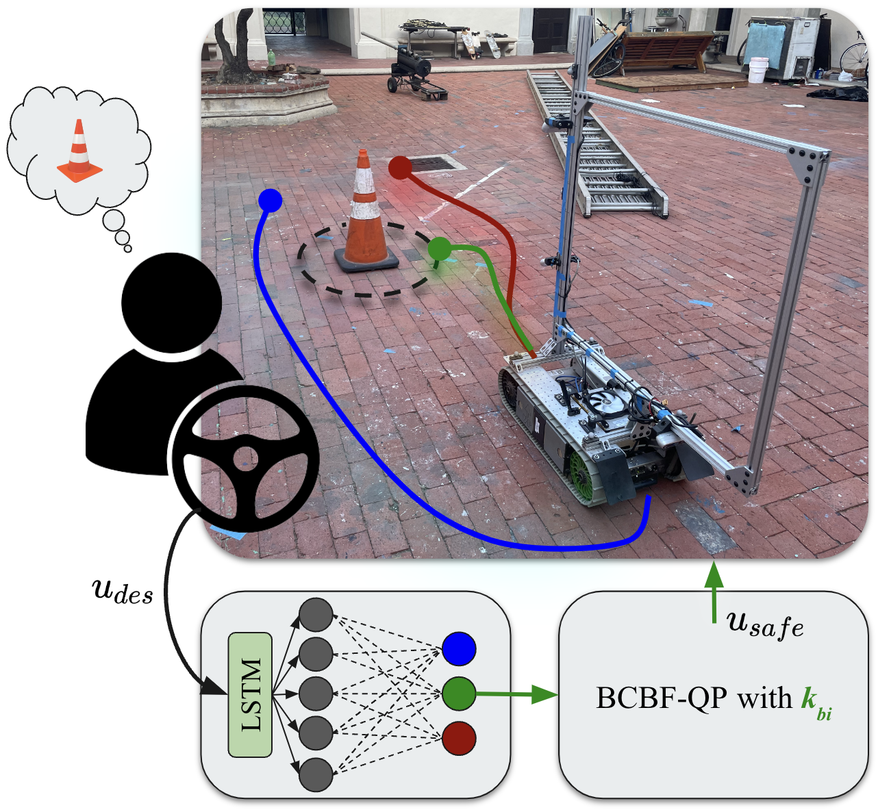
Figure 1: Visualization of the proposed safety-critical control framework with desired robot behavior. The red, green, and blue arrows represent different trajectories that rely on different backup controllers, with corresponding colors, to guarantee safety. Using driver intention tracking, the correct, green, backup controller is chosen among the red and blue controllers in order to guide the driver to their desired location. A supplementary video can be found here: https://youtu.be/41Jh1GD_9Ok

Safety filters are useful control tools that allow a robot to remain safe while under actuation from a potentially unsafe controller, or driver. Safety filters accomplish this by minimally affecting desired control commands, and thus have become a popular add-on to robot control architectures [1, 2, 3] since they address real-world robot dynamics and kinodynamic constraints in a run-time fashion.

Control barrier functions (CBFs) [4] are a popular method for constructing safety filters due to their ability to integrate nonlinear dynamics while providing formal safety guarantees. A CBF-based safety filter requires defining a control-invariant set that ensures safety. However, such sets can be difficult to construct with input constraints in mind [5, 6, 7, 8, 9, 10, 11].

Consequently, the CBF framework has been extended to include actuation capability, such as torque limits, through the use of backup control barrier functions (BCBFs) [12, 13, 14]. BCBFs rely on the formulation of a backup controller, which is designed with input limits in mind to guarantee safety. The backup controller typically involves a simple saving maneuver, such as coming to a stop, turning at a maximum rate, or hovering. By calculating the future backup trajectory of the system, one can analyze future safety of the robot and incorporate this information into optimization-based controllers like quadratic programs (QPs). Consequently, when constructing safety filters using the BCBF method, the system’s conservativeness is a strong function of the control engineer’s choice of backup policy.

To address this limitation, recent work examines the use of multiple backup strategies in the BCBF framework, since multiple strategies can help overcome the conservativeness of a single strategy. In [15], an algorithm is used to evaluate the BCBF method with multiple backup controllers, such that the one with the least control intervention can be chosen. However, with many backup controllers, this method could be computationally infeasible. In [16] and [17], different maneuvers are proposed to increase the reachability of a given backup controller, where a switching algorithm chooses a different maneuver if it is no longer possible to perform the current maneuver. While this method used multiple backup maneuvers with more computationally efficient ways of solving BCBFs, it is better suited to fully autonomous systems. It does not explicitly provide, in a human-robot interaction context, a way to take into account the intentions of a human vehicle driver or human companion. Nor does it account for the fact that the human operator may have better situational awareness than the autonomous controller. Even though autonomous selection may be suboptimal at times, the driver does not have the authority to bypass the chosen backup control strategy. Additionally, it cannot know if the driver has suddenly changed his or her goals. Generally, the types of safe behavior utilized by the BCBF cannot be tuned.

There has been impressive previous work to include human preferences in safety filters. For instance in [18], preference-based learning is used to adapt tuneable parameters of a CBF to user preferences for autonomous obstacle avoidance on a quadruped. However, input bounds are not formally considered, which could potentially result in infeasiblity and consequently unsafe trajectories. While there has also been work on preference based reinforcement learning (pbRL) [19], these methods must sample trajectories within the expected environment [20]. Since the drivers of teleoperated systems must provide control inputs at each timestep, trajectory sampling becomes difficult to complete due to the human-in-the-loop nature of the problem.

In order to intelligently pick backup controllers, we propose a system that utilizes a long short term memory (LSTM) and a deep neural network (DNN) component to learn a reward corresponding to each backup controller. LSTMs have been used in real-time driver intention and maneuver tracking, and have shown to be successful at regression and clasification tasks with trajectory input [21, 22, 23]. A simple switching law is derived by using the controller with the largest reward in the BCBF framework. This system learns to estimate driver intention by training on example trajectories, labeled with the correct choice of backup controller, as provided by the driver. In our work, we show that

1. The LSTM-DNN switching architecture effectively learns the correct backup controller.

2. Our approach increases the reachable sets of the driven robot while maintaining the safety guarantees of BCBFs.

Moreover, we present experimental implementations of our algorithms on a tracked robot. These experiments demonstrate that switching between new and previously formulated backup controllers based on estimated driver intention can work on actual hardware systems.

This paper is organized as follows. Section II presents preliminaries on CBFs, BCBFs, DNNs and LSTMs. Section III presents our contributions, including a description of system architecture. We present the implementation of our framework on hardware in Section IV and discuss experimental results in Section 5. Section VI concludes the paper.

II Preliminaries

We consider robots governed by a general nonlinear control affine system:

$$\dot{x}=f(x)+g(x)u,$$ (1)

where ${x\in\mathbb{R}^{n}}$ is the state, ${u\in U\subset\mathbb{R}^{m}}$ is the control input, and functions ${f:\mathbb{R}^{n}\rightarrow\mathbb{R}^{n}}$, and ${g:\mathbb{R}^{n}\rightarrow\mathbb{R}^{n\times m}}$ are locally Lipschitz continuous. A locally Lipschitz continuous controller ${\mathbf{k}:\mathbb{R}^{n}\to U}$ yields a locally Lipschitz continuous closed-loop control system, ${f_{\rm cl}:X\to\mathbb{R}^{n}}$:

$$\dot{x}={f}(x)+{g}(x)\mathbf{k}(x)\triangleq f_{\rm cl}(x).$$ (2)

Given an initial condition ${x_{0}\triangleq x(t_{0})\in\mathbb{R}^{n}}$, this system has a unique solution given by the flow map

$$\phi(t,x_{0})\triangleq{x}(t)=x_{0}+\int^{t}_{t_{0}}f_{\rm cl}(x(\tau))d\tau,~{}t>t_{0}.$$ (3)

II-A Control Barrier Functions

To characterize safety, we consider a safe set ${\mathcal{C}\subset\mathbb{R}^{n}}$ defined as the 0-superlevel set of a continuously differentiable function ${h:\mathbb{R}^{n}\rightarrow\mathbb{R}}$:

$$\begin{split}\mathcal{C}\triangleq\left\{x\in X\subset\mathbb{R}^{n}:h(x)\geq 0\right\},\\ \partial\mathcal{C}\triangleq\left\{{x\in X\subset\mathbb{R}^{n}}:h(x)=0\right\},\end{split}$$ (4)

where ${\partial\mathcal{C}}$ is the boundary of set $\mathcal{C}$. This set is forward invariant if, for every initial condition ${x(0)\in\mathcal{C}}$, the solution of (2) satisfies ${x(t)\in\mathcal{C},~{}\forall t\geq 0}$. The closed-loop system (2) is called safe w.r.t. set $\mathcal{C}$ if $\mathcal{C}$ is forward invariant [4].

Definition 1 (Control barrier function [4]).

Function $h$ is a CBF for (1) on $\mathcal{C}$ if ${\frac{\partial h}{\partial x}\neq 0}$ for all ${x\in\partial\mathcal{C}}$ and there exists an extended class-$\mathcal{K}_{\infty}$ function $\alpha\in\mathcal{K}_{\infty,e}$ such that $\forall x\in\mathcal{C}$:

$$\sup_{u\in U}\!\Big{[}\!{\dot{h}(x,u)}\!=\!\dfrac{\partial h(x)}{\partial x}\!f(x)\!+\dfrac{\partial h(x)}{\partial x}g(x)\!u\!\Big{]}\!\geq\!-\alpha(h(x)).$$ (5)

Theorem 1.

[4] If $h$ is a CBF for (1) on $\mathcal{C}$, then any locally Lipschitz continuous controller ${\mathbf{k}:\mathbb{R}^{n}\to U}$ satisfying

$$\dot{h}\left(x,\mathbf{k}(x)\right)\geq-\alpha(h(x)),~{}~{}\forall x\in\mathcal{C}$$ (6)

renders (2) safe with respect to $\mathcal{C}$.

II-B Backup Control Barrier Functions

BCBFs are motivated by the fact that verifying (5), which is required for the feasibility of (6), may be challenging for a particular choice of ${h}$, especially with bounded inputs. Consider input bounds with component-wise hard constraints:

$$U\triangleq\left\{u\in\mathbb{R}^{m}:-u_{\rm max}\leq u\leq u_{\rm max}\right\},$$ (7)

where ${u_{\rm max}\in\mathbb{R}^{m}_{>0}}$. The backup set method [12, 13, 14] addresses this feasibility problem by designing implicit control invariant sets and safe controllers through a CBF framework.

We consider a backup set ${\mathcal{C}_{\rm b}\!\subset\!\mathbb{R}^{n}}$ defined as the 0-superlevel set of a continuously differentiable function ${h_{\rm b}:\mathbb{R}^{n}\!\to\!\mathbb{R}}$:

$$\mathcal{C}_{\rm b}\triangleq\left\{x\in\mathbb{R}^{n}:h_{\rm b}(x)\geq 0\right\},$$ (8)

such that it is a subset of ${\mathcal{C}}$, i.e., ${\mathcal{C}_{\rm b}\subseteq\mathcal{C}}$, and ${\frac{\partial h_{\rm b}}{\partial x}\neq 0}$ for all ${x\in\partial\mathcal{C}_{\rm b}}$. Practically speaking, the backup set and backup controller are easily characterized safety procedures that can keep the vehicle in a strict subset of the maximally feasible safe set, which may be impossible to characterize in practice.

We assume that there is a locally Lipschitz continuous backup controller ${\mathbf{k_{b}}:\mathbb{R}^{n}\to U}$, which satisfies (7) for all ${x\in\mathcal{C}}$, to render the backup set forward invariant. This results in the locally Lipschitz continuous closed-loop

$$\dot{x}={f}(x)+{g}(x)\mathbf{k_{b}}(x)\triangleq f_{\rm b}(x),$$ (9)

and its solution with the initial state ${x_{0}\in\mathbb{R}^{n}}$ is

$$\phi_{\rm b}(t,x_{0})\triangleq{x}(t)=x_{0}+\int^{t}_{t_{0}}f_{\rm b}(x(\tau))d\tau,\quad t>t_{0}.$$ (10)

Designing a control invariant backup set ${\mathcal{C}_{\rm b}}$ is generally easier than verifying if ${\mathcal{C}}$ is control invariant. However, the methods used to develop ${\mathcal{C}_{\rm b}}$ may result in a conservative set [5]. We can reduce conservatism by expanding the backup set. To achieve this, we use the backup trajectory ${\phi_{\rm b}(\tau,x)}$ over a finite time period ${\tau\in[0,T]}$ with some ${T\in\mathbb{R}_{>0}}$. Note that ${{\phi_{\rm b}}(\tau,x)}$ is the flow map of the system under the backup controller with the initial condition ${x}$. Then we define a larger control invariant set, called $\mathcal{C}_{E}$, such that ${\mathcal{C}_{\rm b}\subseteq\mathcal{C}_{E}\subseteq\mathcal{C}}$:

$$\begin{split}\mathcal{C}_{E}\triangleq\left\{x\in\mathcal{C}~{}\Bigg{|}\begin{array}[]{ll}\overbrace{h(\phi_{\rm b}(\tau,x)}^{\triangleq\bar{h}_{\tau}(x)}\geq 0,~{}\forall\tau\in[0,T],\\ \underbrace{h_{\rm b}(\phi_{\rm b}(T,x))}_{\triangleq\bar{h}_{\rm b}(x)}\geq 0\end{array}\right\}.\end{split}$$ (11)

That is, $\mathcal{C}_{E}$ is the set of initial states from where the system can use a $T$-length feasible controlled trajectory (that satisfies the input constraints and respects the system dynamics) to safely reach $\mathcal{C}_{\rm b}$. We note that the input limits are satisfied since they are incorporated into the set ${\mathcal{C}_{E}}$ via ${\mathbf{k_{b}}}$. In (11), the first constraint implies that the flow under the backup controller satisfies the safety constraints, and the second constraint enforces that the backup set is reached in time ${T}$. To guarantee safety with respect to $\mathcal{C}_{E}$, we enforce the following constraint for all ${x\in\mathcal{C}_{E}}$:

$$\small\begin{split}\overbrace{\dfrac{\partial h(\phi_{\rm b}(\tau,x))}{\partial\phi_{\rm b}(\tau,x)}\dfrac{\partial\phi_{\rm b}(\tau,x)}{\partial x}f(x)}^{\triangleq L_{f}\bar{h}_{\tau}(x)}\!+\!\overbrace{\dfrac{\partial h(\phi_{\rm b}(\tau,x))}{\partial\phi_{\rm b}(\tau,x)}\dfrac{\partial\phi_{\rm b}(\tau,x)}{\partial x}g(x)}^{\triangleq L_{g}\bar{h}_{\tau}(x)}\!u\\ \geq-\alpha(h(\phi_{\rm b}(\tau,x))),\quad\forall\tau\in[0,T],\\ \underbrace{\dfrac{\partial h_{\rm b}(\phi_{\rm b}(T,x))}{\partial\phi_{\rm b}(T,x)}\dfrac{\partial\phi_{\rm b}(T,x)}{\partial x}f(x)}_{\triangleq L_{f}\bar{h}_{\rm b}(x)}\!+\!\underbrace{\dfrac{\partial h_{\rm b}(\phi_{\rm b}(T,x))}{\partial\phi_{\rm b}(T,x)}\dfrac{\partial\phi_{\rm b}(T,x)}{\partial x}g(x)}_{\triangleq L_{g}\bar{h}_{\rm b}(x)}\!u\\ \geq-\alpha_{\rm b}(h_{\rm b}(\phi_{\rm b}(T,x))).\end{split}$$ (12)

Theorem 2.

[12] Any Lipschitz continuous controller that satisfies (12) keeps the closed loop system (2) safe with respect to $\mathcal{C}_{E}$, which implies ${x(t)\!\in\!\mathcal{C}_{E}\!\subseteq\!\mathcal{C},\forall t\!\geq\!0}$ if ${x_{0}\!\in\!\mathcal{C}_{E}}$.

Note that enforcing the first constraints in (12) is not computationally tractable, as it must hold for all ${\tau\in[0,T]}$. The constraint can be discretized to a finite collection of constraints and then can be directly used for controller synthesis via the following quadratic program (BCBF-QP): |s| u ∈U∥u -k_d(x) ∥^2 k^*(x)​=​ ​​​​L_f ¯h_τ_i(x)​+​L_g ¯h_τ_i(x) u ​≥​-α(h_τ_i(x )) ​​​​L_f ¯h_b(x)​+​L_g ¯h_b(x) u ​≥​-α_b(h_b(x)) for all ${\tau_{i}=iT/N_{\tau},~{}i=0,1,\ldots,N_{\tau}}$, where ${N_{\tau}\in\mathbb{N}}$ is the number of constraints, and ${\mathbf{k_{d}}(x):\mathbb{R}^{n}\to U}$ is a desired controller. In the upcoming experiments, the desired controller is given by the human operator’s vehicle velocity commands.

II-C Deep Neural Networks

We consider an $N_{L}$-layer deep neural network (DNN), ${\Pi:\mathbb{R}^{n_{x}}\rightarrow\mathbb{R}^{n_{y}}}$, which is a piecewise linear function and maps an input feature vector ${\mathbf{\bar{x}}\triangleq(\mathbf{\bar{x}}_{1},\ldots,\mathbf{\bar{x}}_{n_{x}})\in\mathbb{R}^{n_{x}}}$ to an output vector ${\mathbf{\bar{y}}\triangleq(\mathbf{\bar{y}}_{1},\ldots,\mathbf{\bar{y}}_{n_{y}})\in\mathbb{R}^{n_{y}}}$, given by

$$\begin{split}&\upsilon_{\jmath}=\pi_{\jmath}(\mathbf{\bar{W}}_{\jmath}\upsilon_{\jmath-1}+b_{\jmath}),\quad\jmath=1,\ldots,N_{L},\\ &\Pi(\mathbf{\bar{x}})=\mathbf{\bar{y}},\end{split}$$

where $\upsilon_{\jmath}$ is the output of the $\jmath$-th layer of the DNN, and ${\upsilon_{0}=\mathbf{\bar{x}}}$ is the input to the DNN and ${\upsilon_{N_{L}}=\mathbf{\bar{y}}}$ is the output of the DNN, respectively. Each hidden layer has ${n_{\jmath}\in\mathbb{N}}$ hidden neurons. ${\mathbf{\bar{W}}_{\jmath}\in\mathbb{R}^{n_{\jmath}\times n_{\jmath-1}}}$ and ${b_{\jmath}\in\mathbb{R}^{n_{\jmath}}}$ are weight matrices and bias vectors for the $\jmath^{{th}}$ layer, respectively. ${\pi_{\jmath}\triangleq\left[\varrho_{\jmath},\cdots,\varrho_{\jmath}\right]}$ is the concentrated activation functions of the $\jmath^{{th}}$ layer wherein ${\varrho_{\jmath}:\mathbb{R}\rightarrow\mathbb{R}}$ is the activation function, such as sigmoid or ReLU:

$$\varrho_{\textrm{sigmoid}}(\mathbf{\bar{x}}_{j})\triangleq\frac{1}{1+e^{-\mathbf{\bar{x}}_{j}}},\ \ \varrho_{\textrm{ReLU}}(\mathbf{\bar{x}}_{j})\triangleq\max(0,\mathbf{\bar{x}}_{j}).$$

Specifically, we use ${\varrho_{\textrm{sigmoid}}}$ function in our experiments.

II-D Long Short Term Memories

Long Short Term Memories (LSTMs) are a class of Recurrent Neural Networks (RNNs) which have several advantages over DNNs when learning temporally related data. LSTMs also remedy the exploding/vanishing gradient problem of conventonal RNNs by providing a recurrent path for long term memories and another path for short term memories, as the name suggests. LSTM networks [24] learn to map input ${\mathbf{\tilde{x}}=\left[\mathbf{\tilde{x}}_{n\tilde{T}}\right]\in\mathbb{R}^{\tilde{T}n_{x}}}$ to output sequence ${\mathbf{\tilde{y}}=\left[\mathbf{\tilde{y}}_{n\tilde{T}}\right]\in\mathbb{R}^{\tilde{T}n_{y}}}$ for ${n=0,1,\ldots,N}$, where ${\tilde{T}\in\mathbb{R}_{>0}}$ is the sampling time of the LSTM. To learn temporal relationships in this mapping, LSTM units contain a memory cell and four gates: the forget $\mathbf{\tilde{f}}$, input $\mathbf{\tilde{i}}$, output $\mathbf{\tilde{o}}$, and cell $\mathbf{\tilde{c}}$ gates. The recursively defined equations give the outputs of the gate functions:

$$\begin{split}\mathbf{\tilde{f}}_{n}&=\varrho_{\tilde{f}}(\mathbf{\tilde{W}}_{\mathbf{\tilde{f}}}\mathbf{\tilde{x}}_{n}+\mathbf{\tilde{R}}_{\mathbf{\tilde{f}}}\mathbf{\tilde{h}}_{n-1}+\mathbf{\tilde{b}}_{\mathbf{\tilde{f}}}),\\ \mathbf{\tilde{i}}_{n}&=\varrho_{\tilde{f}}(\mathbf{\tilde{W}}_{\mathbf{\tilde{i}}}\mathbf{\tilde{x}}_{n}+\mathbf{\tilde{R}}_{\mathbf{\tilde{i}}}\mathbf{\tilde{h}}_{n-1}+\mathbf{\tilde{b}}_{\mathbf{\tilde{i}}}),\\ \mathbf{\tilde{o}}_{n}&=\varrho_{\tilde{o}}(\mathbf{\tilde{W}}_{\mathbf{\tilde{o}}}\mathbf{\tilde{x}}_{n}+\mathbf{\tilde{R}}_{\mathbf{\tilde{o}}}\mathbf{\tilde{h}}_{n-1}+\mathbf{\tilde{b}}_{\mathbf{\tilde{o}}}),\\ \mathbf{\tilde{g}}_{n}&=\varrho_{\tilde{g}}(\mathbf{\tilde{W}}_{\mathbf{\tilde{g}}}\mathbf{\tilde{x}}_{n}+\mathbf{\tilde{R}}_{\mathbf{\tilde{g}}}\mathbf{\tilde{h}}_{n-1}+\mathbf{\tilde{b}}_{\mathbf{\tilde{g}}}),\end{split}$$

where $n$ and $n-1$ refer to current and previous time steps, ${\varrho_{\tilde{f}},\varrho_{\tilde{i}},\varrho_{\tilde{o}}}$ are the activation functions for input, output and forget gates, and are generally chosen as ${\varrho_{\textrm{sigmoid}}}$. ${\varrho_{\tilde{g}}}$ is the activation function for the memory cell state, which is $tanh$ for general cases, ${\mathbf{\tilde{x}}_{n}}$ is the normalized input, ${\mathbf{\tilde{h}}_{n-1}}$ is the hidden state, and ${\mathbf{\tilde{W}}}$, ${\mathbf{\tilde{R}}}$, ${\mathbf{\tilde{b}}}$ are the weight matrices for $\mathbf{\tilde{i}}$ and the recurrent weight matrices, and bias vectors. The update equations for ${\mathbf{\tilde{h}}_{n-1}}$ and the cell state $\mathbf{\tilde{c}}_{n}$ given by

$$\mathbf{\tilde{h}}_{n}=\mathbf{\tilde{o}}_{n}\odot\varrho_{\tilde{g}}(\mathbf{\tilde{c}}_{n});\ \ \mathbf{\tilde{c}}_{n}=\mathbf{\tilde{f}}_{n}\odot\mathbf{\tilde{c}}_{n-1}+\mathbf{\tilde{i}}_{n}\odot\mathbf{\tilde{g}}_{n},$$

where $\odot$ is the Hadamard (element-wise) product.

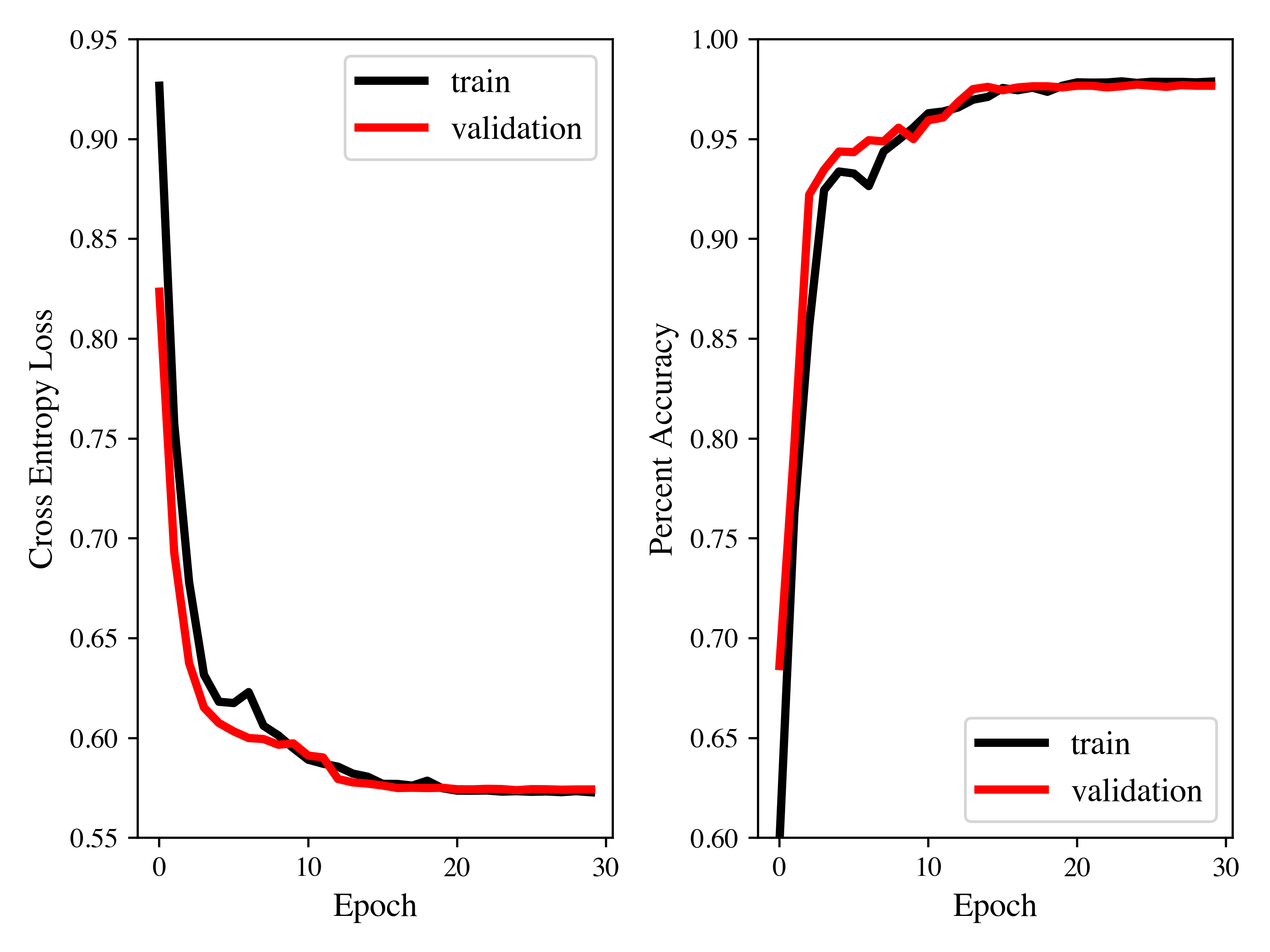
Figure 2: Cross entropy and training loss during a training episode. Accuracy is calculated by comparing the maximum reward ouput from the LSTM-DNN architecture and determining if it corresponds to the correct choice of backup controller for the respective point in the training set. We also use a validation (test) dataset to observe out-of-sample performance of the network during training. The network achieves 97% accuracy by the 30th epoch.

Then, with a fully connected layer, weight matrix ${\mathbf{\tilde{W}}_{y}}$ and bias vector ${\mathbf{\tilde{b}}_{y}}$, the output of the LSTM network is given by

$$\mathbf{\tilde{y}}=\mathbf{\tilde{W}}_{y}\mathbf{\tilde{h}}_{n}+\mathbf{\tilde{b}}_{y}.$$

Notably, ${\mathbf{\tilde{W}}}$ and ${\mathbf{\tilde{b}}}$ do not vary with $n$, as the feedback loop nature of LSTMs and RNNs allow the same weights and biases to be used for each timestep in a sequence of data. This allows LSTMs and RNNs to be applied on input sequences of varying lengths without changes in architecture.

III Intention Estimation

To improve the reachability of multiple BCBFs through intention estimation, a deep LSTM-DNN network translates observational data from the driver, safety systems, and robot state into the choice of $\mathbf{k_{b}}$.

For organizational purposes, the following sections that describe our framework use the following definitions

• $\mathcal{K}$ is a set of $m_{k}\in\mathbb{N}$ backup controllers such that controller $\mathbf{k_{bi}}\in\mathcal{K}$ renders a backup set $\mathcal{C}_{{\rm b}i}\subseteq\mathcal{C}$ forward invariant

• $\gamma_{t}\in\mathbb{R}^{k}$ is a vector of ${k\in\mathbb{N}}$ features: robot state, environment, driver input, and safety data. We maintain an ${H+1}$-length data history ${\vec{\gamma}(t,H)=(\gamma_{t},\gamma_{t-1},\ldots,\gamma_{t-H})}$, Additional details on $\vec{\gamma}(t,H)$ can be found below.

• $R:\mathbb{R}^{k\times(H+1)}\to\mathbb{R}^{m_{k}}$ is a reward function that maps input history $(\gamma_{t},\gamma_{t-1},\ldots,\gamma_{t-H})$ to a list of $m_{k}$ rewards with values ranging from 0 to 1. Each component of this list corresponds to the integer $i$ of each controller $\mathbf{k_{bi}}\in\mathcal{K}$.

We use a unicycle model to capture the tracked robot’s motion, given by

$$\underbrace{\begin{bmatrix}\dot{x}_{I}\\ \dot{y}_{I}\\ \dot{\theta}\end{bmatrix}}_{\dot{x}}=\underbrace{\begin{bmatrix}0\\ 0\\ 0\end{bmatrix}}_{{f}(x)}+\underbrace{\begin{bmatrix}\cos{\theta}&0\\ \sin{\theta}&0\\ 0&1\end{bmatrix}}_{{g}(x)}\underbrace{\begin{bmatrix}v\\ \omega\end{bmatrix}}_{u},$$ (13)

where ${p=\begin{bmatrix}{x}_{I}&{y}_{I}\end{bmatrix}^{\top}}$ is the vehicle’s planar position w.r.t. the inertial frame ${I}$, $\theta$ is vehicle’s yaw angle, ${-v_{\rm max}\leq v\leq v_{\rm max}}$ is its linear velocity and ${-\omega_{\rm max}\leq\omega\leq\omega_{\rm max}}$ is the angular velocity. While we describe our intention estimator in the context of the unicycle model, we believe that our system can generalize to more complex dynamical models. This is the subject of future experimentation as detailed in section VI.

We employ an intention estimation framework to learn the reward function, $R$. Learning is useful in this context since constructing a reward function based on multi-modal input in high dimensions may be challenging. The feature vector at a single timestep, ${\gamma_{t}}$, consists of the robot state and vertical position ${[x^{I},z^{I}]\in\mathbb{R}^{4}}$, robot state and vertical velocities ${[\dot{x}^{I},\dot{z}^{I}]\in\mathbb{R}^{4}}$, driver velocity commands ${u\in U}$, and safety information from evaluating ${h:\mathbb{R}^{3}\to\mathbb{R}}$ at $x$ and at ${x_{g}\in\mathbb{R}^{3}}$, which is an intermediate goal determined by forward integrating the driver’s desired $u$ over a short horizon. Note that $\gamma_{t}$ can contain many more features than detailed here in other implementations, especially if they relate to the safety of the robot. However, the aforementioned features generalize to any robot using our implementation. We wish to learn $R$ by mapping history $\vec{\gamma}(t,H)$ to rewards corresponding to each backup controller $\mathbf{k_{bi}}$ at time $t$. This process allows us to derive switching laws for the chosen backup controller as a function of time. For instance, we may choose the backup controller $\mathbf{k_{bi}}$ with the largest reward at time $t$ where $i=\operatorname*{arg\,max}(R(\vec{\gamma}(t,H))$

We use a deep LSTM network with a DNN decoder to construct $R$ from history $\vec{\gamma}(t,H)$. Deep LSTMs can learn complex temporal relationships by using multiple layers and cyclic connections to understand sequential data, and the DNN decoder maps the output of the LSTM to rewards for each backup controller through several hidden layers. Both the LSTM and DNN utilize dropout for regularization, and the DNN uses ReLU activations in the hidden layers. Furthermore, we use the sigmoidal activation function in the DNN final layer. Thus, the outputted rewards for each backup controller, $\mathbf{k_{bi}}$ at time $t$, can be interpreted very loosely as a likelihood that $\mathbf{k_{bi}}$ is a correct backup controller choice at time $t$. For example, if our framework is highly certain that $\mathbf{k_{b0}}$ is the correct choice of backup controller at time $t$, then the first component of the output of ${R(\vec{\gamma}(t,H))}$ is expected to be close to 1.

Our strategy and architecture enables easy reward engineering for the training dataset. We construct a multi-class dataset by gathering data of the robot driving in suitable environments under the correct backup controllers. During data collection the robot should be operating with a BCBF safety filter as we plan to evaluate the network in safety-critical contexts. During training, the switches between backup controllers are labeled in the dataset by the driver using configurable buttons on the robot ground station. Labeling is completed by assigning $1$ to the driver’s choice of backup controller and $0$ to all others for that instance. Since we utilize the sigmoidal activation function in this multi-class classification learning task, we use the softmax loss function to train the network. Indeed, this training procedure makes an implicit assumption that there exists a single, correct choice of backup controller at any given time. While this may not be true in certain situations, we guarantee safe switching as discussed in Section IV-B. Consequently, any choice of correct backup controller, or switch between them, does not void safety guarantees. We discuss discontinuities between switching controllers in section 5, however in short, switching between backup controllers is, in practice, smooth.

To improve training, we utilize the Adam optimizer [25] with a stepped learning rate scheduler that reduces the learning rate every constant step of training epochs. In order to compensate for the time it takes to solve the BCBF-QP, we employ a forecast of roughly double the time it takes our system to solve the BCBF-QP. In other words, before training we shift backup controller labels backwards in time so that the network learns to pre-emptively select the correct backup controller, allowing time for the BCBF-QP to have computed safe control outputs for the new controller when they are needed. We show results from a training episode done on hardware-collected data in Fig. 2, and present our model parameters here. We used a 2 layer LSTM with 100 hidden units with the 12 total input features detailed earlier. Our DNN is composed of two hidden layers of sizes 50 and 25 neurons, respectively. We use a dropout value of 0.2 for the hidden layers of the DNN and a dropout of 0.1 for the LSTM. As indicated in Fig. 2, we achieved $97\%$ accuracy over a dataset of 19000 datapoints collected on hardware. The sequence length for the training samples of the LSTM-DNN model was chosen to be 15 timesteps, which corresponds to roughly 0.75 seconds of data. We found that this time-range produced the most accurate results in the aforementioned offline training.

III-A Human Interface

Since we extract an intention estimation signal from the human driver, providing necessary feedback is essential for improving human-robot collaboration. Past work has suggested that systems which allow robots to estimate human intention, while their collaborating humans estimate robot intention, can improve overall performance [26]. Thus, we develop an interface based on the ROS rviz visualization tool as well as an Xbox controller featuring haptic motors. The rviz system displays a visualization of the robot pose, along with dials that indicate estimated system safety, as quantified by the magnitude of the saturated safety function $tanh(h(x))$. Furthermore, vibratory haptic feedback is provided to the user when the robot nears the boundary of the safe set as indicated by $h$. This feedback warns that the vehicle is in a potentially dangerous conditions, so we tune the the thresholds and strength of the haptic feedback as preferred by the driver.

IV Implementation

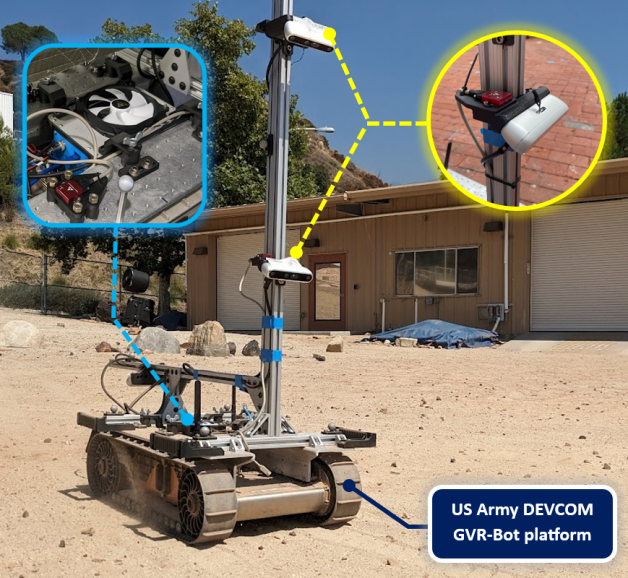
Figure 3: Photo of our test-vehicle (a US Army DEVCOM GVR-Bot robot) operating in the NASA Jet Propulsion Laboratory Mars Yard. $(yellow\ inset)$ Intel Realsense D457 Depth Cameras are coupled with a VN-100 IMU, $(light-blue\ inset)$ custom compute payload.

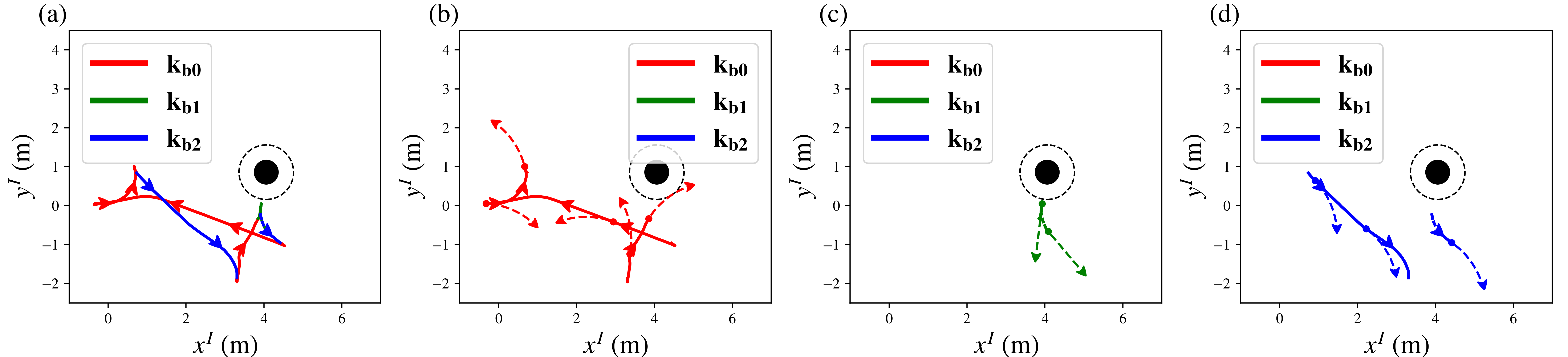
Figure 4: Robot trajectory which used all three backup controllers under our learned switching law. Subfigure (a) shows the robot trajectory, where direction is indicated by the arrows and the choice of backup controller is indicated by color. Subfigures (b), (c), and (d) show the segments of the robot trajectory that used $\mathbf{k_{b1}},\mathbf{k_{b2}},\mathbf{k_{b3}}$ respectively. In (b), (c), and (d) we also show the flows of the respective backup controllers at several robot positions. Notice that in each of (b) (c) (d), the backup controller flow always escapes the obstacle. However, notice that $\mathbf{k_{b0}}$ may not provide safe evasion from the obstacle in the locations in subfigure (c) as it does for the locations in (b). This implies that our system chose the correct backup controller depending on several factors, like driver intent and robot position.

IV-A Hardware

Our algorithms are deployed on a tracked GVR-Bot from US Army DEVCOM Ground Vehicle Systems Center. The GVR-Bot is a modified iRobot PackBot 510 and its rugged design and quick actuation makes it ideal for research of safety in the presence of unknown human driver intentions. Our Python and C++ algorithms run on a custom compute payload that is based on an NVIDIA Jetson AGX Orin (2048-core NVIDIA Ampere architecture, 64 Tensor Cores, 275 TOPS, 12 Core Arm Cortex A78AE @ 2.2GHz, 32GB Ram). Vision is provided by three synchronized Intel Realsense D457 Depth Cameras which are strategically positioned to provide a wide field of view for the control system and operator. They operate at a 30 Hz frame rate. A Vectornav VN-100 provides inertial measurements. Communication between our algorithm, the control computer, and the internal GVR-Bot drive computer (Intel Atom) is facilitated via ROS1. Estimation of the vehicle state is provided by an OpenVINS visual-inertial estimator [27]. Drive commands (linear and angular body velocities) are communicated from the AGX Orin to the Intel Atom where they are converted into individual track speeds, which are regulated via high-rate controllers on the GVR-Bot, see Fig. 1 and Fig. 3.

IV-B Backup Controllers

For safety, the tracked robot must avoid moving obstacles, considered as cylinders with radius ${R_{o}\in\mathbb{R}_{>0}}$, position ${p_{o}\in\mathbb{R}^{2}}$ and velocity ${v_{o}\in\mathbb{R}^{2}}$. This leads to the safety constraint ${h(x)\geq 0}$, with the CBF candidate given by

$$h(x)=\|p-p_{o}\|-R_{o}.$$

We enforce safety in the presence of input bounds by implementing multiple BCBFs.

We leverage three backup controllers that yield qualitatively different behavior. Controller $\mathbf{k_{b0}}$ turns the robot away from the obstacle and drives away with maximum speed. Controller $\mathbf{k_{b1}}$ drives straight away as the obstacle is approached, without turning. Controller $\mathbf{k_{b2}}$ turns towards the obstacle and drives in reverse. It behaves similarly to $\mathbf{k_{b0}}$, however the robot has turned around. These are expressed by:

$$\mathbf{k_{b}}(x)=\begin{bmatrix}v_{\rm max}\\ \omega_{\rm max}\tanh(n^{T}r/\varepsilon)\end{bmatrix},\;\;h_{0}(x)=n^{T}(qv_{\rm max}-v_{o}),$$

$$\mathbf{k_{b1}}(x)=\begin{bmatrix}v_{\rm max}\tanh(n^{T}q/\varepsilon)\\ 0\end{bmatrix},\;\;h_{1}(x)=\|p-p_{o}\|-R_{o},$$

$$\mathbf{k_{b2}}(x)=-\mathbf{k_{b0}}(x),\hskip 56.9055pth_{2}(x)=-h_{0}(x),$$

where $\tanh$ is used to obtain smooth policies with smoothing parameter ${\varepsilon\in\mathbb{R}_{>0}}$, and the vectors $n$, $q$, $r$ are given by:

$$n=\frac{p-p_{o}}{\|p-p_{o}\|},\quad q=\begin{bmatrix}\cos\theta\\ \sin\theta\end{bmatrix},\quad r=\begin{bmatrix}-\sin\theta\\ \cos\theta\end{bmatrix}.$$ (14)

Each policy maintains a forward invariant backup set, i.e., the 0-superlevel set of the BCBF $h_{0}$, $h_{1}$ and $h_{2}$. These sets represent the states where the robot faces away from the obstacle (for $h_{0}$), the robot has positive distance from the obstacle ($h_{1}$), and it faces towards the obstacle ($h_{2}$).

Ultimately, the BCBFs enable the robot to maintain safe behavior. At the same time, the performance can be improved by switching between the backup policies based on learning. Safety must be preserved when switching between multiple backup controllers. Consider a switch from backup controller $\mathbf{k_{bi}}$ to $\mathbf{k_{bj}}$. One way to ensure safety during this crossover is to evaluate constraints (12) for the new controller $\mathbf{k_{bj}}$. We are guaranteed to be in the $T$-time reachable set of the first controller, $\mathbf{k_{bi}}$. Thus, validating that the BCBF-QP constraints hold for $\mathbf{k_{bj}}$ in practice requires that both backup controllers’ $T$-time reachable sets intersect. Furthermore, note that if backup controllers with $T$-time reachable sets are the only controllers switched between, the resulting QPs will always be feasible. This has the effect of, in practice, resulting in relatively smooth switching between controllers.

V Results

Figure 5: Demonstration of system safety during switches between backup controllers. See that $h(x)\geq 0$ and the input constraints are satisfied (denoted by the gray dotted lines); therefore, our system maintains safety while better aligning with driver intention.

(a)

(b)

(c)

Figure 6: We compare our system on multiple environments with the use of a single backup controller, and also show the reproducibility of our test data. In figure (a), we attempt to drive the robot forwards to a point on the far right of the obstacle. In figure (b), we drive the robot and face the obstacle at various points. In figure (c), we attempt to reach the same goal as figure (a), but by driving the robot backwards. Notice our system provides more gentle corrections to driver controls and enables the driver to reach the goal position in every case.

By referring to Fig. 4, it is evident from the alternating colors that our learned reward function selected multiple backup controllers over a single robot trajectory. Our framework also selected appropriate backup controllers such that robot reachability near the obstacle was maximized. Furthermore, our system maintains the formal safety guarantees from the BCBF method as demonstrated in Fig. 5, where $h$ was observed to be positive under input limits. To demonstrate the reproducibility of these results, further tests were conducted and documented in Fig. 6 and the accompanying video shared in the caption of Fig 1. Here, we tested our system in many scenarios and compared produced trajectories to trajectories corresponding to a single backup controller. The use of our switching framework outperforms the use of a single backup controller in certain scenarios, and our system never inhibits the driver from achieving their goal, while some backup controllers do. For instance, sub-figure (b) of Fig 6 presents a case where $\mathbf{k_{b0}}$ inhibited the driver while our framework did not. The learned reward function correctly captures the driver’s intent, encompassing risk-neutral preferences such as emergency stopping and overtaking with minimal slowdown, as well as risk-averse behaviors like maintaining a sizeable safety distance.

VI Conclusions and Future Work

In this work, we implemented backup control barrier functions to ensure safety on a tracked robot platform, and used driver intention estimationto optimally choose between multiple backup policies. From our results, we conclude that this system improves safety and performance by improving the interaction between the robot and its driver by expanding the multiple BCBF framework with a learning method.

Several next steps exist for this preliminary framework, like, developing an algorithm to formally compute safe reachability under multiple backup controllers. Furthermore, while we showed that our framework is useful on a teleoperated ground vehicle, we plan to implement our framework on other robots, such as quadrupeds, bipeds, and drones. Finally, various techniques can be employed to enhance the resilience of standard CBF constraint (6) against disturbance or model uncertainty, such as GP-based uncertainty in the CBF constraint [28], [29].

Acknowledgment. The authors would like to thank the SFP program at Caltech, SFP sponsors Kiyo and Eiko Tomiyasu, and DARPA for funding this project. Furthermore, the authors would like to thank Ryan K. Cosner and Maegan Tucker for discussions about safety with backup CBFs and learning, and Matthew Anderson for his insights and help in experimental setup and testing.

References

- [1] K. L. Hobbs, M. L. Mote, M. C. Abate, S. D. Coogan, and E. M. Feron, “Runtime assurance for safety-critical systems: An introduction to safety filtering approaches for complex control systems,” IEEE Control Systems Magazine, vol. 43, no. 2, pp. 28–65, 2023.
- [2] K.-C. Hsu, H. Hu, and J. F. Fisac, “The safety filter: A unified view of safety-critical control in autonomous systems,” arXiv preprint arXiv:2309.05837, 2023.
- [3] K. P. Wabersich and M. N. Zeilinger, “A predictive safety filter for learning-based control of constrained nonlinear dynamical systems,” Automatica, vol. 129, p. 109597, 2021.
- [4] A. D. Ames, X. Xu, J. W. Grizzle, and P. Tabuada, “Control barrier function based quadratic programs for safety critical systems,” Transactions on Automatic Control, vol. 62, no. 8, pp. 3861–3876, 2017.
- [5] Y. Chen, M. Jankovic, M. Santillo, and A. D. Ames, “Backup control barrier functions: Formulation and comparative study,” in 2021 60th IEEE Conference on Decision and Control (CDC). IEEE, 2021, pp. 6835–6841.
- [6] J. Breeden and D. Panagou, “Robust control barrier functions under high relative degree and input constraints for satellite trajectories,” Automatica, vol. 155, p. 111109, 2023.
- [7] D. R. Agrawal and D. Panagou, “Safe control synthesis via input constrained control barrier functions,” in 2021 60th IEEE Conference on Decision and Control (CDC). IEEE, 2021, pp. 6113–6118.
- [8] W. S. Cortez and D. V. Dimarogonas, “Correct-by-design control barrier functions for Euler-Lagrange systems with input constraints,” in 2020 American Control Conference (ACC). IEEE, 2020, pp. 950–955.
- [9] W. Xiao, C. A. Belta, and C. G. Cassandras, “Sufficient conditions for feasibility of optimal control problems using control barrier functions,” Automatica, vol. 135, p. 109960, 2022.
- [10] A. Wiltz, X. Tan, and D. V. Dimarogonas, “Construction of control barrier functions using predictions with finite horizon,” arXiv preprint arXiv:2305.05294, 2023.
- [11] C. Folkestad, Y. Chen, A. D. Ames, and J. W. Burdick, “Data-driven safety-critical control: Synthesizing control barrier functions with Koopman operators,” IEEE Control Systems Letters, vol. 5, no. 6, pp. 2012–2017, 2020.
- [12] T. Gurriet, M. Mote, A. Singletary, P. Nilsson, E. Feron, and A. D. Ames, “A scalable safety critical control framework for nonlinear systems,” IEEE Access, vol. 8, pp. 187 249–187 275, 2020.
- [13] T. G. Molnar and A. D. Ames, “Safety-critical control with bounded inputs via reduced order models,” in 2023 American Control Conference (ACC). IEEE, 2023, pp. 1414–1421.
- [14] R. K. Cosner, A. W. Singletary, A. J. Taylor, T. G. Molnar, K. L. Bouman, and A. D. Ames, “Measurement-robust control barrier functions: Certainty in safety with uncertainty in state,” in 2021 IEEE/RSJ International Conference on Intelligent Robots and Systems (IROS). IEEE, 2021, pp. 6286–6291.
- [15] Y. Chen, A. Singletary, and A. D. Ames, “Guaranteed obstacle avoidance for multi-robot operations with limited actuation: A control barrier function approach,” IEEE Control Systems Letters, vol. 5, no. 1, pp. 127–132, 2021.
- [16] A. Singletary, A. Swann, I. D. J. Rodriguez, and A. D. Ames, “Safe drone flight with time-varying backup controllers,” in 2022 IEEE/RSJ International Conference on Intelligent Robots and Systems (IROS). IEEE, 2022, pp. 4577–4584.
- [17] A. Singletary, A. Swann, Y. Chen, and A. D. Ames, “Onboard safety guarantees for racing drones: High-speed geofencing with control barrier functions,” IEEE Robotics and Automation Letters, vol. 7, no. 2, pp. 2897–2904, 2022.
- [18] R. Cosner, M. Tucker, A. Taylor, K. Li, T. Molnar, W. Ubelacker, A. Alan, G. Orosz, Y. Yue, and A. Ames, “Safety-aware preference-based learning for safety-critical control,” in Learning for Dynamics and Control Conference. PMLR, 2022, pp. 1020–1033.
- [19] E. R. Novoseller, Y. Wei, Y. Sui, Y. Yue, and J. W. Burdick1, “Dueling posterior sampling for preference-based reinforcement learning,” in Conference on Uncertainty in Artificial Intelligence, 2020, pp. 1029–1038.
- [20] C. Wirth, R. Akrour, G. Neumann, and J. Fürnkranz, “A survey of preference-based reinforcement learning methods,” Journal of Machine Learning Research, vol. 18, no. 136, pp. 1–46, 2017. [Online]. Available: http://jmlr.org/papers/v18/16-634.html
- [21] N. Khairdoost, M. Shirpour, M. A. Bauer, and S. S. Beauchemin, “Real-time driver maneuver prediction using lstm,” IEEE Transactions on Intelligent Vehicles, vol. 5, no. 4, pp. 714–724, 2020.
- [22] S. Wang, X. Zhao, Q. Yu, and T. Yuan, “Identification of driver braking intention based on long short-term memory (lstm) network,” IEEE Access, vol. 8, pp. 180 422–180 432, 2020.
- [23] A. Zyner, S. Worrall, J. Ward, and E. Nebot, “Long short term memory for driver intent prediction,” in 2017 IEEE Intelligent Vehicles Symposium (IV), 2017, pp. 1484–1489.
- [24] F. A. Gers and J. Schmidhuber, “Recurrent nets that time and count,” in International Joint Conference on Neural Networks, 2000, pp. 189–194.
- [25] D. P. Kingma and J. Ba, “Adam: A method for stochastic optimization,” arXiv preprint arXiv:1412.6980, 2014.
- [26] A. D. Dragan, S. Bauman, J. Forlizzi, and S. S. Srinivasa, “Effects of robot motion on human-robot collaboration,” in 2015 10th ACM/IEEE International Conference on Human-Robot Interaction (HRI), 2015, pp. 51–58.
- [27] P. Geneva, K. Eckenhoff, W. Lee, Y. Yang, and G. Huang, “OpenVINS: A research platform for visual-inertial estimation,” in 2020 IEEE International Conference on Robotics and Automation (ICRA), 2020, pp. 4666–4672.
- [28] F. Castaneda, J. J. Choi, B. Zhang, C. J. Tomlin, and K. Sreenath, “Gaussian process-based min-norm stabilizing controller for control-affine systems with uncertain input effects and dynamics,” in 2021 American Control Conference (ACC). IEEE, 2021, pp. 3683–3690.
- [29] F. Castañeda, J. J. Choi, B. Zhang, C. J. Tomlin, and K. Sreenath, “Pointwise feasibility of Gaussian process-based safety-critical control under model uncertainty,” in 2021 60th IEEE Conference on Decision and Control (CDC). IEEE, 2021, pp. 6762–6769.