Computation-Limited Signals: A Channel Capacity Regime Constrained by Computational Complexity

Abstract

In this letter, we introduce the computational-limited (comp-limited) signals, a communication capacity regime in which the signal time computational complexity overhead is the key constraint – rather than power or bandwidth – to the overall communication capacity. We present the Spectro-Computational (SC) analysis, a novel mathematical framework that enhances classic concepts of information theory – such as throughput, spectral efficiency and capacity – to account for the signal processing computational complexity overhead. We consider a specific Shannon regime under which capacity is expected to get arbitrarily large as channel resources grow. Under that regime, we identify the conditions under which the time complexity overhead causes capacity to decrease rather than increasing, thereby creating the case for the comp-limited regime. We also provide examples of the SC analysis and show the OFDM waveform is comp-limited unless the lower-bound computational complexity of the $N$-point DFT problem verifies as $\Omega(N)$, which remains an open challenge.

I Introduction

Information theory introduces power and bandwidth as the fundamental resources to describe the capacity of a noisy channel. The development of clever physical layer techniques associated to the adoption of larger spectrum resources have provided new wireless telecommunication standards with unprecedented data rates. As a consequence, the computational resources required to process more bits per signal has grown accordingly, highlighting the trade-off between the signal processing computational complexity and the signal data rate. Despite of that, as far as we know, few knowledge have been produced to equate these performance indicators.

Some research efforts propose unified models of computation and information theory but without concerning about the interplay between the signal processing time complexity and capacity. For instance, works such as [1] concern about whether a discrete (Turing) machine is able to compute a given channel capacity function. Other works bring the term “complexity” to information theory but with different meaning than that of the computation complexity. This is the case of the communication complexity theory [2] and the “Kolmogorov complexity” [3], in which the term stands for the minimum number of message exchanges to solve a problem in a distributed manner and the length of the irreducible form of an information, respectively.

In this letter, we present an analytical framework referred to as the “Spectro-Computational (SC) analysis”. With the SC analysis, we revisit classic concepts of information theory – such as throughput, spectral efficiency and capacity – in order to account for the signal processing computational complexity overhead. Our mathematical framework enhances and generalizes concepts we previously propose to study the complexity-throughput trade-off lying in the context of specific waveforms [4], [5], [6], [7]. Based on that, we refer to a specific Shannon capacity regime to derive a novel capacity regime in which computational complexity matters more than channel resources such as bandwidth of received power.

The remainder of this letter is organized as follows. In Section II, we review the background and present the rationale for our mathematical framework. In Section III, we present the mathematical framework of the SC analysis. In Section IV, we formalize the comp-limited communication regime. In Section V, we present practical examples of the SC analysis. In Section VI we present our conclusion and future work.

II Background and Rationale

In this section, we review some key properties of asymptotic notation that will support our analyses throughout this work (subsection II-A). In subsection II-B, we present the rationale of our proposal by discussing the interplay between computational complexity and channel resources in the Shannon communication system.

II-A Asymptotic Notation

The asymptotic analysis relate functions $f(N)$ and $g(N)$ as $N\to\infty$. For the quantities of this work, we assume increasing non-negative functions. We follow the classic notation popular in the literature of analysis of algorithms.Thus, if $f(N)=\Theta(N)$, $f(N)=o(g(N))$ and $f(N)=\omega(g(N))$, it denotes that the order of growth of $f(N)$ is equal to, strictly higher than, or strictly less than the order of growth of $g(N)$, respectively. Similarly, if $f(N)=O(g(N))$ then $f(N)=o(N)$ or $f(N)=\Theta(N)$ and $f(N)=\Omega(g(N))$ implies that $f(N)=\omega(N)$ or $f(N)=\Theta(N)$. Thus, all asymptotic notations can be defined according to Eqs. (1), assuming existing limits and a real constant $c>0$.

$$c, f(N)=\Theta(g(N))$$ if (1a)

$$0, f(N)=o(g(N))$$ if (1b)

$$\infty, f(N)=\omega(g(N))$$ if (1c)

II-B A Case for a Time Complexity-Constrained Signal Regime

In this subsection, we firstly review the channel resources considered by Shannon to describe the capacity regimes. Then, we argue how these channel resources are related to the signal processing computational complexity and argue for a time complexity-constrained capacity regime.

II-B1 Shannon Capacity Regimes

Let us consider the Additive Gaussian White Noise (AWGN) channel capacity formula of Shannon, based on which the two classic channel capacity regimes of information theory derives from, namely, the Bandwidth-Limited Regime (BLR) and Power-Limited Regime (PLR). According to Shannon, the capacity of an AWGN channel is

$$C = W\log_{2}(1+\mathsf{SNR})\quad\mathrm{bits/second}$$ (2)

$$\mathsf{SNR} = \frac{\mathcal{P}}{WN_{0}}$$ (3)

where $W$ is the channel bandwidth, $\mathsf{SNR}$ is the Signal-to-Noise Ratio (SNR), $\mathcal{P}$ is the received signal power and $N_{0}$ is the noise power spectral density. Eq. (2), establishes an upper bound for the data rate $R$ experienced by a $B(W)$-bit message in an AWGN-constrained channel. In other words, for a symbol period of $T_{\text{sym}}$, data rate $R$ and the spectral efficiency $SE$ are given in Eq. (4) and Eq. (5), respectively.

$$R = \frac{B(W)}{T_{\text{sym}}}<C\quad\text{bits/second}$$ (4)

$$SE = \frac{R}{W}<C\quad\text{bits/second/Hertz}$$ (5)

in which $T_{\text{sym}}$ is the signal period. PLR results when SNR is very small ($\mathsf{SNR}\ll 1$). In this case, one can approximate $\log_{2}(1+\mathsf{SNR})$ as $\mathsf{SNR}\log_{2}e$, thereby $C$ becomes linear on $\mathcal{P}$ and is not affected by $W$. If SNR remains high ($\mathsf{SNR}\gg 1$) as $W$ grows, $C$ becomes proportional to $W$, leading to the BLR case. Note, however, that widening $W$ for a fixed $\mathcal{P}$ impairs SNR due to the resulting overall noise. In this case, the regime changes from BLR to PLR as $W$ grows.

II-B2 Channel Resources and Time Complexity

Beyond power and spectrum, computational resources are also intrinsic to the Shannon’s communication system. In fact, in that system, a transmitter/receiver must be able to “operate on the message in some way to produce a signal” [8]. Specially when digital communication systems take place (our focus in this work), the computational resources consumed by such operation depend on length of the transmitting message which, in turn, is dimensioned according to the channel resources. Therefore, capacity regimes such as BLR and PLR directly affect the implied computational complexity. By its turn, such complexity overhead can impair time-related performance indicators (e.g., throughput, capacity) if properly considered in the analysis.

II-B3 What If Channel Resources Grow Arbitrarily?

To illustrate how time complexity can affect communication performance, consider the Shannon capacity formula (Eq. 2) under the fixed SNR regime with $\mathcal{P}\geq WN_{0}$ (Eq. 3). As $W\to\infty$, $\mathcal{P}\to\infty$ accordingly to counter the resulting noise and keep the SNR constant. Thus, in this case, $C=cW$ for some constant $c>0$, i.e., $C=\Theta(W)$ (Eq. 1a), meaning that Shannon predicts an infinite capacity as channel resources grow in the fixed SNR regime ($\mathcal{P}\geq WN_{0}$). In other words, $\lim_{W\to\infty,\mathcal{P}\to\infty}C=\infty\quad\text{bits/second}$.

Let us now considering the effect of the time complexity in the analysis. Let $T(W)$ denote the number of computational instructions required to turn the $B(W)$-bit message into a $W$ Hertz signal. For a finite baseband processor (we discuss and formalize this assumption in Section III)), each instruction takes a runtime of $t>0$ seconds. If one accounts for the time complexity overhead in the throughput, the classic data rate formula of Eq. (4) rewrites as

$$R = \frac{B(W)}{tT(W)+T_{\text{sym}}}<C\quad\text{bits/second}$$ (6)

Under arbitrarily large channel resources as in the fixed SNR regime, both of the ratio $B(W)$ and $T(W)$ tends to infinity. In this case, since $t$ does not depend on $W$ and $T_{\text{sym}}$ is bounded by a constant – to ensure higher sampling rate as $W$ grows –, the computational-constrained data rate solely depends on the ratio $B(W)/T(W)$ as $W\to\infty$. If $B(W)$ grows faster than $T(W)$, i.e., $B(W)=\omega(T(W))$, then $R_{W\to\infty}=B(W)/T(W)=\infty$ (Eq. 1c), as expected by the Shannon fixed SNR regime. However, if $B(W)=o(T(W))$ then $R_{W\to\infty}=B(W)/T(W)=0$ (Eq. 1b). Therefore, differently from expected by the information theory, there might be regimes in which the growth of the channel resources might cause capacity to decrease (rather than increase) if the limits imposed by computational complexity are considered..

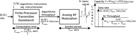
Figure 1: Communication system model of the SC analysis (receiver-side omitted).

III Fundamentals of Spectro-Computational Complexity

Throughout this section, we evolve the classic definitions of information theory to account for the signal processing time complexity overhead. The resulting analytical framework we refer to as the “SC” analysis. The term “SC” dates back to our earliest work [7], in which we concerned about the trade-off between spectral efficiency and computational complexity lying in a specific waveform. To avoid ambiguity with the classic definitions, we will adopt the same nomenclature of our original work to designate each novel enhanced definition. Therefore, in what follows, we revisit the classic information theory definitions of data rate $R$ (or throughput, Eq. 4) and spectral efficiency $SE$ (Eq. 5) to introduce the enhanced homologous concepts of “SC throughput” $SC_{R}$ (Eq. 9) and “SC efficiency” $SC_{SE}$ (Eq. 11), respectively. We leave the definition of the “SC capacity” to Section IV.

III-1 System Model and Assumptions

Fig. 1 illustrates the transmitter of our communication system for a $W$-Hertz channel. The analysis is reciprocal for the receiver side. We concern about the throughput experienced by a particular $B(W)$-bit message. The message is turned into a baseband signal by a “finite-baseband transmitter” that can perform $\mathcal{I}>0$ instructions per second. Note that $\mathcal{I}$ represents the computational resource which is assumed as finite. Thus, considering fundamental limits of baseband processor manufacturing [9], we assume $\mathcal{I}$ cannot be made arbitrarily large as the channel resources $W$ and $P$ grow.

To turn the message into a signal, $T(W)$ computational instructions are required (i.e., ‘time complexity’). $T(W)$ can be set according to the convenience of the analysis. For example, it can represent all instructions or only the asymptotically dominant (most frequent). Also, it can either represent the complexity of a single algorithm or all signal baseband algorithms. Note that the algorithmic input length always depend on $B(W)$ which, in turn, depends on $W$. Thus, in any case, the complexity $T$ can always be written as function of $W$.

III-2 Computational Time and Algorithmic Throughput

The signal baseband processing runtime $T_{\text{comp}}$ and the algorithmic throughput $A(W)$ of the baseband processor in Fig. 1 are defined in Eq. (7) and Eq. (9), respectively.

$$T_{\text{comp}} = \frac{T(W)}{\mathcal{I}}\quad\text{seconds}$$ (7)

$$A(W) = \frac{B(W)}{T_{\text{comp}}}=\frac{\mathcal{I}B(W)}{T(W)}\quad\text{bits/second}$$ (8)

The “Analog RF Modulation” block converts the signal to analog and performs the carrier modulation. The entire process corresponds to the symbol duration $T_{\text{sym}}$ seconds.

III-3 Spectro-Computational Throughput

Thus, in addition to $T_{\text{comp}}$, the signal carrying the $B(W)$-bit message will take $T_{\text{sym}}$. Based on this, we define the SC data rate (or throughput) $SC_{R}(W)$ as

$$SC_{R}(W)=\frac{B(W)}{T_{\text{comp}}+T_{\text{sym}}}=\frac{B(W)}{\displaystyle\frac{T(W)}{\mathcal{I}}+T_{\text{sym}}}\quad\text{bits/second}$$ (9)

As usual in the analysis of algorithms, one may focus on the number of algorithmic instructions $T(W)$ without concerning about the time a single instruction takes on a particular processor. This can be reflected in Eq. (8) and Eq. (9) by setting $\mathcal{I}=1$. Besides, one may also neglect the constants involved for the convenience of the asymptotic analysis. Under these assumptions, observe that

$$A(W)=SC_{R}(W)=\frac{B(W)}{T(W)}\quad\text{bits/instruction}$$ (10)

For this reason, we consider the terms algorithmic throughput and SC throughput interchangeable. Similarly, note that the rate units bits/instruction and bits/second are interchangeable. This results either because the number of seconds match the number of instructions under $\mathcal{I}=1$ or if constants are neglected for the sake of the asymptotic analysis of Eqs. (8) and (9). As in our prior works [5], [6], we assume these conditions unless otherwise stated.

III-4 Spectro-Computational Efficiency

Based on the SC throughput (Eq. 9), we introduce the SC Efficiency (SCE) to enhance the classic definition of SE (Eq. 5) with time complexity. This is given in Eq. (11).

$$SC_{SE}(W) = \frac{SC_{R}(W)}{W}\quad\text{bits/second/Hertz}$$ (11)

which can also be given in bits/instruction/Hertz if $\mathcal{I}=1$. Next, we build on the definitions of this section to formalize a novel capacity regime.

IV Computation-Limited Signals

In this section, we build upon the definitions of Section III to define the SC capacity. Based on this, we formalize a novel capacity regime we refer to as computation-limited signals.

IV-A SC Algorithmic Capacity

We define the SC (algorithmic) capacity $SC_{C}(W)$ of a waveform as an asymptotic upper bound for the SC throughput $SC_{R}(W)$ of Eq. (9), i.e., $SC_{R}(W)=O(SC_{C}(W))$. Assuming the fixed SNR regime discussed in Section II-B3, $W\to\infty$ and the constants $\mathcal{I}$ and $T_{\text{sym}}$ of Eq. (9) can be ignored. Thus, our analysis follows based on $SC_{R}(W)$ of Eq. 10. In that case, the upper-bound $SC_{C}(W)$ is defined as the ratio

$$SC_{C}(W) = \frac{B_{\text{max}}(W)}{\mathcal{L}(W)}\quad\text{bits/second}$$ (12)

and

$$SC_{R}(W) = O(SC_{C}(W))$$ (13)

In Eq. (12), $B_{\text{max}}(W)$ and $\mathcal{L}(W)$ stand for the highest and lowest orders of growth that can be assumed for the numerator $B(W)$ and the denominator $T(W)$, respectively. In practice, $B_{\text{max}}(W)$ can be set to the maximum number of bits possible in a given waveform. In general terms, we approximate $B_{\text{max}}(W)$ asymptotically as $\Theta(C)$. Under the fixed SNR regime, it results

$$B_{\text{max}}(W)=\Theta(C)=cW\quad\text{bits}$$ (14)

In turn, $\mathcal{L}(W)$ is known as the asymptotic lower bound of a computational problem. By times, such function is hard to derive since it is conditioned to identification of the asymptotically fastest algorithm ever for the considered problem. For example, it is widely known that the current fastest known algorithm for the $N$-point DFT problem runs in $O(N\log_{2}N)$ time. However, whether this is the lowest complexity ever (i.e., $\mathcal{L}(W)=\Theta(N\log_{2}N)$) remains an open question in theoretical computer science (we discuss this case in Section V).

IV-B The Comp-Limited Signal Regime

To ensure the SC throughput does not nullify as the channel resources grow, the waveform design might satisfy Lemma 1.

Lemma 1 (Condition of Scalability)

Under the fixed SNR regime discussed in Section II-B3, the SC throughput (Eq. 10) nullifies as $W\to\infty$ unless $B(W)=\Omega(T(W))$.
The condition of scalability is such that

$$SC_{R}(W\to\infty)=\lim_{W\to\infty}\frac{B(W)}{T(W)} > 0,$$ (15)

To ensure Ineq. 15 holds, the time complexity must grow as fast as $B(W)$ at most, i.e. $B(W)=\Omega(T(W))$. It means either $B(W)=\Theta(T(W))$ (Eq. 1a) or $B(W)=\omega(T(W))$ (Eq. 1c). If none of these cases holds, then $B(W)=o(T(W))$ does, since the conditions of Eq. 1 are mutually exclusive. Under this latter case, it follows from Eq. (1b) that $SC_{R}(W\to\infty)=0$. Therefore, the SC throughput $SC_{R}(W)$ nullifies as $W\to\infty$ unless $B(W)=\Omega(T(W))$. $\blacksquare$

A given waveform implementation may not satisfy Lemma 1. In some cases, overcoming that is just a matter of devising and implementing asymptotically faster baseband algorithms e.g., [5]. We are particularly interested in checking whether the SC capacity $SC_{C}(W)$ of a waveform meets Lemma 15. If it does not, then the waveform design is constrained by computational complexity since the time complexity cannot be improved in $SC_{C}(W)$. We define this as the comp-limited regime.

Definition 1 (Comp-Limited Signal Regime)

A signal waveform is limited by computation (comp-limited) if its SC (algorithmic) capacity $SC_{C}(W)$ (Eq. 12) does not meet Lemma 1.

Def. 1 translates the fact that there exist conditions under which the computational resources of the baseband processor must grow arbitrarily (i.e., $\mathcal{I}\to\infty$) to prevent the time complexity to nullify capacity as $W\to\infty$. Therefore, in this regime, capacity is limited by the computational – rather than spectrum or power – resources.

V Examples

In this section, we demonstrate different use cases of the SC analysis. In particular, we resort to our SC analysis mathematical framework to show how to perform equitable data rate comparison with baseband processors of different computational resources. Then, we analyze whether the data rate of OFDM waveform is limited by the computational resources as the number of subcarriers grows.

V-A Common Parameters

For the analyses of this section, we assume a $N$-subcarrier OFDM signal spaced by $\Delta f$ Hz and with a symbol period of $T_{\text{sym}}=1/\Delta f$ seconds. For an $M$-point constellation diagram, the number of bits of the OFDM frame is $B(N)_{OFDM}=N\log_{2}M$. However, for the analyses of this section, we assume $B(N)_{OFDM}=N$ bits without loss of generality.

V-B A Fairer Wi-Fi Data Rate Comparison

Figure 2: FFT baseband processor comparison: 512-point (right-hand side) vs. 64-point (left-hand side) (apud [10]). The 512-point processor achieves $8\times$ higher throughput at the penalty of consuming larger computational resources. We show this gain nearly halves if the extra computational resources is allocated for both cases.

The IEEE 802.11ac standard supports $8\times$ faster data rates in comparison to its IEEE 802.11a counterpart. This results from widening the bandwidth by a factor of $8\times$ keeping the legacy OFDM symbol period of $T_{\text{sym}}=3.2$ $\mu$s unchanged (without considering cyclic prefix, CP). However, such an improvement comes at a cost. Consider, for example, a DFT computation of roughly $T_{DFT}(N)=N\log_{2}N$ algorithmic instructions [4]. Thus, increasing $N$ from $64$ (IEEE 802.11a) to $512$ (IEEE 802.11ac) causes a non-negligible impairment of roughly $T_{DFT}(512)/T_{DFT}(64)=12\times$ in time complexity.

Regardless of that, the total computation time $T_{\text{comp}}$ (Eq. 7) must finish in $T_{\text{sym}}$ seconds to ensure a real-time signal processing in each case. To meet this, the number of instructions per second performed by the baseband processor must grow as function of the bandwidth. In other words, more computational resources are assigned to the $N=512$ case, thereby impairing other (non temporal) performance indicators such as manufacturing cost, chip area (portability) and power consumption. This is clearly illustrated in Fig. 2. As we show next, the $8\times$ data rate gain of the 512-point baseband processor decreases to $\approx 4\times$ if the 64-point case is fairly provided the same superior computational resources.

With the SC analysis, we calculate the data rate for the $N=64$ case assuming the same computational resources $\mathcal{I}_{512}$ of the $N=512$ case. Considering $T_{comp}=3.2\mu$s, it results $\mathcal{I}_{512}=T_{DFT}(512)/3.2=1440$ instructions/microsecond (Eq. 7) and $SC_{R}(512)=512/6.4=80$ bits/microsecond (Eq. 9). Under the same computational resources, the $N=64$ case achieves a faster runtime of $T_{\text{comp}}=T_{DFT}(64)/1440\approx 0.266$ microseconds and, consequently, a faster data rate of $SC_{R}(64)=64/3.46\approx 18.46$ bits/microsecond. Therefore, if the additional computational resources are equitably allocated in both scenarios, the data rate gain of the wider signal becomes $SC_{R}(512)/SC_{R}(64)\approx 4.3$, which is nearly half of what is expected when time complexity is overlooked.

V-C Is OFDM a Comp-Limited Signal?

Next, we present a step-by-step analysis of the SC capacity of OFDM to answer whether it classifies as a comp-limited signal.

V-C1 Asymptotic model

As in the prior sections, our reference model is the fixed SNR regime of Shannon in which $W\to\infty$. Translated to OFDM, it means that $N\to\infty$ since both $T_{\text{sym}}$ and, consequently, $\Delta f$ are assumed as constants. Besides, because SNR is constant in the regime, the number of bits per subcarrier $\log_{2}M$ is also constant as $N$ grows.

V-C2 Max. Number of OFDM Bits $B_{\text{max}}(N\to\infty)_{OFDM}$

Hence, the maximum number of bits per OFDM frame as $N$ grows is $B_{\text{max}}(N\to\infty)_{OFDM}=cN$ for some real constant $c>0$.

V-C3 Complexity of $T_{OFDM}(N\to\infty)$

The overall time complexity $T_{OFDM}(N\to\infty)$ of the uncoded OFDM signal results from the complexity of its individual procedures, namely, (de)mapping, (I)DFT computation, addition/deletion of CP, signal detection, and equalization. Of these, DFT and signal detection are popularly known as the most complex. However, by recalling that the input for the signal detection is the number of pilots (which is usually a fraction of $N$) and considering a low complex estimator (such as the Least Squares, LS), the DFT computation becomes the most complex procedure of OFDM. Therefore, as $N$ grows, the constants and the complexities of all other procedures can be neglected for the sake of the asymptotic analysis. Please, note that one can proceed the SC analysis of any OFDM algorithm since the unique requisites for that are the waveform parameters (i.e., the number of bits and the symbol duration) and the complexity of the considered algorithm(s). To avoid unnecessary intricacy, we set the asymptotic complexity $T_{OFDM}(N)$ of OFDM to the complexity $T_{DFT}(N)$ of the DFT algorithm.

V-C4 SC Capacity of OFDM $SC_{C}(N)_{OFDM}$

Unfortunately, we cannot define the SC capacity of OFDM because the lower bound complexity of the DFT problem remains open. However, considering the conjectures of $\Omega(N\log_{2}N)$ and $\Omega(N)$ [4], Theorem 1 follows.

Theorem 1 (Comp-Limited OFDM Signal)

The uncoded OFDM signal is comp-limited unless the $N$-point DFT problem can be solved in linear time complexity.
Proof: Suppose the fastest algorithm for the DFT problem runs in $O(N\log_{2}N)$ time complexity. Then, the SC capacity of OFDM is $SC_{C}(N\to\infty)_{OFDM}=N/(N\log_{2}N)=0$. In this case, OFDM is a comp-limited signal according to Def. 1. Following that Def., the lower bound complexity should be linear in $N$ – because it requires $T_{DFT}(N)=O(B_{\text{max}}(N)_{OFDM})=O(N)$)–, which matches the conjecture of $\Omega(N)$. In fact, if $T_{DFT}(N)=\Omega(N)$ then $SC_{C}(N\to\infty)_{OFDM}=c_{1}$ for some constant $c_{1}>0$. Therefore, the uncoded OFDM signal is comp-limited unless the $N$-point DFT problem can be solved in linear time complexity.

Theorem 1 further motivates the research to answer whether the $N$-point DFT problem is $\Omega(N)$, which remains an open question in theoretical computer science [4].

VI Conclusion and Future Work

In this letter, we proposed a mathematical framework to enhance performance indicators from the information theory to account for the signal processing time complexity overhead. We demonstrated how these concepts are intrinsically related and can affect one another. We concerned about why time complexity is overlooked in classic formulas of information theory such as data rate and variants thereof. One potential explanation we posited for that stems from the fact that runtime (i.e., number of instructions/second) is countered at the penalty of other non temporal performance indicators (like manufacturing cost and chip area). This way, the impact of the time complexity overhead on those classic formulas is assumed as negligible. Through a case study of our framework, we showed that the data rate gain expected from widening the bandwidth can nearly halve if its extra computational resources is also allocated to the baseband processor of the narrower counterpart signal. In other case study, we demonstrated that the computational resources can be more crucial for capacity than the channel resources like bandwidth or received power. We referred to such capacity regime as comp-limited signals. Regarding this, we showed that the uncoded OFDM signal is comp-limited unless the lower-bound complexity of the $N$-point DFT problem verifies as $\Omega(N)$. Future work may further enhance our model to account for the interplay between time complexity and bit error rate in algorithms such as error correction codes.

References

- [1] R. F. Schaefer, H. Boche, and H. V. Poor, “Turing Meets Shannon: On the Algorithmic Computability of the Capacities of Secure Communication Systems (Invited Paper),” in 2019 IEEE 20th International Workshop on Signal Processing Advances in Wireless Communications (SPAWC), 2019, pp. 1–5.
- [2] A. Rao and A. Yehudayoff, Communication Complexity: and Applications. Cambridge University Press, 2020.
- [3] G. J. Chaitin, Algorithmic Information Theory, ser. Cambridge Tracts in Theoretical Computer Science. Cambridge University Press, 1987.
- [4] S. Queiroz, J. P. Vilela, and E. Monteiro, “Is FFT Fast Enough for Beyond 5G Communications? A Throughput-Complexity Analysis for OFDM Signals,” IEEE Access, vol. 10, pp. 104 436–104 448, 2022.
- [5] S. Queiroz, W. Silva, J. P. Vilela, and E. Monteiro, “Maximal spectral efficiency of OFDM with index modulation under polynomial space complexity,” IEEE Wireless Communications Letters, vol. 9, no. 5, pp. 1–4, 2020.
- [6] S. Queiroz, J. P. Vilela, and E. Monteiro, “Optimal Mapper for OFDM With Index Modulation: A Spectro-Computational Analysis,” IEEE Access, vol. 8, pp. 68 365–68 378, 2020.
- [7] S. Queiroz, J. Vilela, and E. Monteiro, “What is the cost of the index selector task for OFDM with index modulation?” in IFIP/IEEE Wireless Days (WD) 2019, Manchester, UK, Apr. 2019.
- [8] C. E. Shannon, “A mathematical theory of communication.” Bell Syst. Tech. J., vol. 27, no. 3, pp. 379–423, 1948.
- [9] G. E. Moore, “No exponential is forever: but “forever” can be delayed! [semiconductor industry],” in 2003 IEEE International Solid-State Circuits Conference, 2003. Digest of Technical Papers. ISSCC., 2003, pp. 20–23 vol.1.
- [10] S. Queiroz, “Spectro-computational complexity analysis for wireless communications,” Ph.D. dissertation, 00500:: University of Coimbra, 2022.