2+1D symmetry-topological-order from local symmetric operators in 1+1D
Abstract
A generalized symmetry (defined by the algebra of local symmetric operators) can go beyond group or higher group description. A theory of generalized symmetry (up to holo-equivalence) was developed in terms of symmetry-TO – a bosonic topological order (TO) with gappable boundary in one higher dimension. We propose a general method to compute the 2+1D symmetry-TO from the local symmetric operators in 1+1D systems. Our theory is based on the commutant patch operators, which are extended operators constructed as products and sums of local symmetric operators. A commutant patch operator commutes with all local symmetric operators away from its boundary. We argue that topological invariants associated with anyon diagrams in 2+1D can be computed as contracted products of commutant patch operators in 1+1D. In particular, we give concrete formulae for several topological invariants in terms of commutant patch operators. Topological invariants computed from patch operators include those beyond modular data, such as the link invariants associated with the Borromean rings and the Whitehead link. These results suggest that the algebra of commutant patch operators is described by 2+1D symmetry-TO. Based on our analysis, we also argue briefly that the commutant patch operators would serve as order parameters for gapped phases with finite symmetries.
I Introduction
Topological order [1] is a collection of low energy universal properties of gapped liquid [2, 3] phases of matter, which are captured by topological quantum field theories [4, 5], or by non-degenerate braided fusion higher categories [6]. These phases are physically characterized by the algebraic properties of various topological excitations. For example, topological orders in 2+1 dimensions are classified by the fusion and braiding of topological point-like excitations known as anyons [7, 8, 9, 10, 11], which are generally described by modular tensor categories [12, 5] (see, e.g., [13, 14] for a review). Categorical descriptions and classifications of topological orders in higher dimensions are also developed recently in [6, 15, 16, 17, 18].
After the systematic understanding of gapped liquid phases of matter, we like to gain a systematic understanding of gapless liquid phases of matter with linear dispersion, which is a long-standing challenge in theoretical physics. One way to make progress [19] is to study a key invariant of gapless liquid phases – the low energy emergent symmetry. The emergent symmetry can be a generalized symmetry, which is a combination of ordinary group-like symmetries, anomalous symmetries [20], higher-form symmetries [21, 22, 23], higher-group symmetries [24, 25, 26, 27], and more general non-invertible 0-symmetries [28, 29, 30, 31, 32, 33, 34, 35, 36, 37, 38, 39, 40, 41] and non-invertible higher symmetries [42, 43, 44].111Non-invertible symmetries in higher dimensions have been studied intensively over the past few years following the seminal work of [45, 46], see, e.g., [47, 48, 49, 50, 51] for reviews. In fact, we can use non-invertible gravitational anomalies [52, 53, 54, 55, 56, 57] to describe all the above different emergent generalized symmetries in a unified way [58, 42, 43, 44]. Since gravitational anomalies correspond to topological orders in one higher dimension [52, 55, 56], this leads to symmetry/topological-order (Symm/TO) correspondence [58, 42, 43, 44].
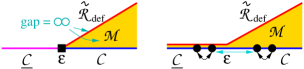
The relation between topological orders and generalized symmetries becomes manifest in the isomorphic holographic decomposition described by Fig. 1 [55, 58, 42, 43, 44, 60]. The composite system (a slab of bulk topological order with a gapped boundary and a low energy boundary ) exactly simulates the low energy system , for example and have the same partition function, in the limit where the gaps of and approach infinity. If a low energy theory has such an isomorphic holographic decomposition, then the has an emergent symmetry described by and (where is the generalized Drinfeld center). If is a local fusion higher category, then the symmetry (which is usually non-invertible) is an anomaly-free algebraic higher symmetry [42, 43] (or a fusion category symmetry for 1+1D case [41]). If is not local, then the symmetry is anomalous.
If we only look at the symmetry within the symmetric sub-Hilbert space , then some different symmetries, such as symmetry with mixed anomaly and symmetry in 1+1D [61, 62], become equivalent, which is called holo-equivalent [43]. It was proposed that a holo-equivalence class of symmetries is described fully by symmetry-TO in one higher dimension [58, 43].222Mathematically, two fusion higher categories, and , describe holo-equivalent symmetries if they are Morita equivalent . The symmetry-TO was called “categorical symmetry” in [58, 43]. Thus, symmetry-TO (and its mathematical description – braided fusion higher category in the trivial Witt class), replacing group and higher group, becomes a theory for generalized symmetry (up to holo-equivalence). Such a holographic picture was discussed for 1+1D in, e.g., [57, 41, 58, 63, 64, 65, 61, 66, 67, 68, 69]. The holographic picture was also used to study dualities [70]. See Sec. III.1 for more details of the holographic picture of symmetries. The symmetry-TO is also called a symmetry topological field theory (symmetry-TFT) [71]. The name “symmetry-TO” stresses the existence of lattice UV completion and the absence of any lattice symmetry.
We know that a (generalized) symmetry is defined by an algebra of local symmetric operators without involving anything in one higher dimension. Ref. 58, 61, 72 try to calculate the braided fusion higher category from the local symmetric operators directly. Usually, one introduces commutant operators that commute with all the local symmetric operators, and then uses the algebra of commutant operators to describe and define symmetry. But here, to calculate braided fusion higher category, Ref. 61, 72 introduced commutant patch operators. A commutant patch operator is formed by local symmetric operators glued together on a patch of any dimension.333In the examples discussed in [58, 61], a commutant patch operator reduces to the product of local symmetric operators on a patch. It commutes with all the local symmetric operators far away from the boundary of the patch. Moreover, it is a symmetric operator by itself because it consists of local symmetric operators. Ref. 61, 72 conjecture that the algebra of commutant patch operators encodes a braided fusion higher category, which in turn describes a symmetry-TO if the braided fusion higher category is finite. A similar idea is also presented in [73, 74], where it was shown that certain 1+1D lattice models with Morita equivalent symmetries have isomorphic algebras of symmetric local operators. A related problem is also studied in the context of algebraic quantum field theory [75] under the name of the DHR theory [76, 77, 78, 79], see, e.g., [80, 81, 82] for the reconstruction of 2+1D topological orders from 1+1D quantum spin chains in this context.
The conjecture in [61] implies that the data of topological orders are encoded in the algebra of commutant patch operators in one lower dimension. Indeed, in [58, 61], the anyon data of the 2+1D toric code and double-semion topological orders were explicitly computed from commutant patch operators in 1+1D systems with non-anomalous and anomalous symmetries. A similar computation of the anyon data of the toric code was also performed in [83] based on topological excitations in 1+1D gapped phases with non-anomalous symmetry. This computation was later generalized to the case of an arbitrary non-anomalous abelian group symmetry in [84]. The above results motivate us to expect that it would be possible to reconstruct more general topological orders from commutant patch operators in one lower dimension. However, thus far, topological orders that have been explicitly reconstructed from patch operators are limited to several abelian topological orders mentioned above.
In this paper, we generalize the analysis in [58, 61] so that we can reconstruct more general 2+1D topological orders from 1+1D systems with finite symmetries that are generally described by fusion categories [39, 40, 41]. In particular, based on the holographic picture of 1+1D systems with finite symmetries, we will argue that the anyon data of 2+1D topological orders should be encoded in commutant patch operators in 1+1 dimensions. The commutant patch operators will also be called symmetric transparent connectable patch operators in the subsequent sections due to the properties of these operators.444The name “transparent patch operator” was coined in [61] to emphasize that a commutant patch operator is transparent to local symmetric operators away from its boundary. We will then propose a general method to compute the anyon data of 2+1D topological orders from these patch operators. As an example, we will write down symmetric transparent connectable patch operators in 1+1D systems with a general non-anomalous finite group symmetry and verify our proposal by explicitly computing the anyon data of the corresponding topological orders in 2+1D. The anyon data that we will compute include topological invariants beyond modular data, such as those associated with the Borromean rings and the Whitehead link.
The rest of the paper is organized as follows. In Sec. II, we will give a brief review of topological orders in 2+1 dimensions. In Sec. III, we will propose a general scheme to compute the anyon data of 2+1D topological orders by using symmetric transparent connectable patch operators in 1+1 dimensions. In Sec. IV, we will apply our computational scheme to the topological order realized by Kitaev’s quantum double model for a general finite group. More specifically, we will demonstrate that various topological invariants associated with anyon diagrams of Kitaev’s quantum double model can be computed from patch operators in 1+1D systems with finite group symmetry. In Sec. V, we will summarize the results and argue that symmetric transparent connectable patch operators would serve as order and disorder operators for gapped phases with finite symmetries. In App. A, we will discuss a relation between patch operators in 1+1D systems with a finite group symmetry and ribbon operators on the rough boundary of Kitaev’s quantum double model. Throughout the paper, we will only consider bosonic systems.
II Review of topological orders in 2+1 dimensions
In this section, we briefly review the algebraic description of 2+1D topological orders.
II.1 General case
It is widely believed that topological orders in 2+1 dimensions (up to invertible ones) are mathematically described by non-degenerate braided fusion categories, which axiomatize the fusion and braiding statistics of anyons. The basic data of a non-degenerate braided fusion category consist of the following ingredients (see, e.g., [85, 14, 86] for more details):
-
•
A finite set of anyon types . This set is equipped with an involution , where is called the dual of . The distinguished element corresponds to a trivial anyon.
-
•
Fusion rules , where is a non-negative integer called a fusion coefficient. The trivial anyon behaves as a unit under the fusion, i.e., .
-
•
Finite dimensional vector spaces and called a fusion space and a splitting space, whose dimensions are equal to the fusion coefficient . Elements of these vector spaces are called morphisms.
-
•
-symbols that describe the crossing relations of worldlines of anyons:
(1) The summation on the right-hand side is taken over fusion channels and basis morphisms and . The -symbols must satisfy consistency conditions known as the pentagon equation [85]. We note that the -symbols are not gauge invariant, i.e., they depend on the choice of bases of the splitting spaces.
-
•
-symbols that describe the braiding of anyon lines:
(2) The summation on the right-hand side is taken over basis morphisms . The -symbols must satisfy consistency conditions known as the hexagon equations [85]. We note that the -symbols are also gauge dependent.
-
•
A left evaluation morphism and a left coevaluation morphism that describe the annihilation and creation of a pair of anyons:
(3) where the worldline of is represented by the orientation reversal of that of . The evaluation and coevaluation morphisms must satisfy the following zigzag identities:
(4) -
•
A right evaluation morphism and a right coevaluation morphism represented by the diagrams
(5) which satisfy the zigzag identities analogous to Eq. (4). In a unitary (braided) fusion category, the left and right evaluation/coevaluation morphisms are related by the Hermitian conjugation.
Given a non-degenerate braided fusion category, we can associate a complex number with any closed diagram consisting of anyon lines. This complex number can be expressed in terms of the -symbols, -symbols, and evaluation/coevaluation morphisms. In particular, when anyon lines form a framed knot or link, the associated complex number is gauge invariant. We will call such a gauge invariant quantity simply a topological invariant. Of particular importance among topological invariants are the following quantities:
-
•
The quantum dimension of each anyon . This is a topological invariant associated with a loop of an anyon line:
(6) The quantum dimension in a unitary (braided) fusion category is a positive real number that is greater than or equal to one. When , is called an abelian anyon. Otherwise, it is called a non-abelian anyon.
-
•
The topological spin of each anyon . This is a topological invariant associated with an anyon line forming a figure of eight:
(7) -
•
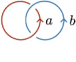
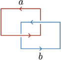
The -component of the modular -matrix for each pair of anyons and . This is a topological invariant associated with the Hopf link:
(8) Here, is the total dimension. The modular -matrix is non-degenerate in a non-degenerate braided fusion category.
The topological spins and modular -matrix are called modular data.
Although the modular data largely characterize a non-degenerate braided fusion category, they are not complete invariants. Namely, different non-degenerate braided fusion categories can have the same modular data [87]. Several topological invariants have been proposed to distinguish topological orders that share the same modular data [88, 89, 90, 91, 92]. We may expect that the set of all topological invariants associated with framed knots and links of anyon lines uniquely determines a non-degenerate braided fusion category. However, a simple set of topological invariants that completely characterize a non-degenerate braided fusion category has not been worked out yet.
A 2+1D topological order is said to be non-chiral if it admits a topological (i.e., gapped) boundary condition, while it is chiral otherwise. Mathematically, a 2+1D topological order is non-chiral if and only if the non-degenerate braided fusion category describing anyons is equivalent to the Drinfeld center of a fusion category [93, 94]. In general, 2+1D non-chiral topological orders are realized by the Levin-Wen model [95], whose low energy limit is described by the Turaev-Viro-Barrett-Westbury topological field theory [96, 97]. In the rest of this paper, we will only consider non-chiral topological orders due to their intimate relation to finite symmetries in 1+1D.
II.2 Example: Kitaev’s quantum double topological order
A simple example of a 2+1D topological order is realized by Kitaev’s quantum double model [98], which is a Hamiltonian formulation of a topological finite gauge theory known as the (untwisted) Dijkgraaf-Witten theory [99].555In general, we can twist Kitaev’s quantum double model by a third group cohomology [100]. The topological order of this model is described by the topological gauge theory with the Dijkgraaf-Witten twist [99]. We will not consider such a twisted version of the quantum double model in this paper. We will denote Kitaev’s quantum double model based on a finite group as . In this subsection, we summarize the anyon data of Kitaev’s quantum double model , or equivalently, a topological -gauge theory (see, e.g., [101] for a review).
The anyons of the quantum double model are labeled by pairs , where is the conjugacy class of and is a unitary irreducible representation of the centralizer of .
-
•
The quantum dimension of an anyon labeled by is given by
(9) where is the number of elements in and is the dimension of the representation .
-
•
The topological spin of an anyon is given by
(10) where, by a slight abuse of notation, denotes the representation matrix of and the trace is taken over the representation space of .
-
•
The -component of the modular -matrix is given by
(11) where and are the complex conjugate representations of and respectively. The group element is a representative of a coset in , i.e., an arbitrary element that satisfies for .
The complete anyon data of Kitaev’s quantum double model is described by the representation category of the quantum double of group algebra [98]. This category is equivalent to the Drinfeld center of the category of -graded vector spaces as a braided fusion category, see, e.g., [86].
When is abelian, anyons of Kitaev’s quantum double model are labeled by pairs of a group element and a unitary irreducible representation of because the conjugacy class of consists only of and the centralizer of is the whole group . Since any irreducible representation of a finite abelian group is one-dimensional, Eq. (9) implies that all anyons of Kitaev’s quantum double model for an abelian group have quantum dimension one, i.e., they are abelian anyons. Furthermore, the topological spins and modular -matrix in this case reduce to and respectively.
III Topological orders in 2+1D from patch operators in 1+1D
A patch operator in 1+1 dimensions is an extended operator that acts only on a finite interval (i.e., a patch) of a one-dimensional space. In this section, we propose a general method to compute topological invariants of 2+1D non-chiral topological orders by using patch operators in 1+1D systems with finite symmetries. The basic idea of computing topological invariants from patch operators was already presented in [58, 61], where it was demonstrated that the modular data of several abelian topological orders, such as the toric code and double-semion topological orders, can be computed from patch operators in one lower dimension. Here, we will slightly extend the formulation in [58, 61] so that we can also deal with non-abelian topological orders. In what follows, topological orders are assumed to be non-chiral and have an infinitely large energy gap unless otherwise stated.
III.1 Motivation
We first provide motivation behind our expectation that the anyon data of a 2+1D topological order should be encoded in patch operators in 1+1D systems with finite symmetry. To this end, we first recall the holographic picture that we mentioned in Sec. I. As illustrated in Fig. 2, a 1+1D system with finite symmetry can be obtained by putting a 2+1D topological order on a slab , where is a finite interval and is a two-dimensional oriented surface [70, 41, 63, 64, 65, 60, 44]. On the left boundary of the slab, we impose a topological boundary condition, while on the right boundary, we impose a non-topological physical boundary condition.
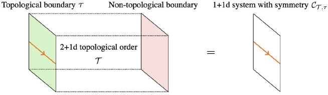
The symmetry of the 1+1D system obtained in this way is described by a fusion category formed by topological lines on the left boundary . We denote this fusion category by , where is the 2+1D topological order in the bulk and is the topological boundary condition on the left. To be more precise, the 1+1D system has symmetry if we view the system from the left side of the 2+1D bulk.666If we look at the 1+1D system from the other side of the bulk, the symmetry is described by the opposite category . The fusion category and the bulk topological order are related by the boundary-bulk relation, i.e., the bulk topological order is described by the Drinfeld center of [102, 103, 93, 104].777A similar boundary-bulk relation also holds in higher dimensions [105, 106].
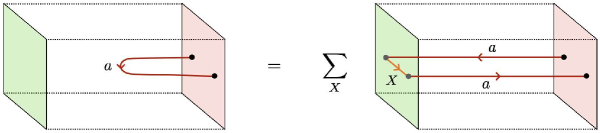
The relation between anyons in the bulk topological order and patch operators in 1+1D is now clear: a bulk anyon line terminating on the right boundary gives rise to a patch operator of the 1+1D system, see Fig. 3.
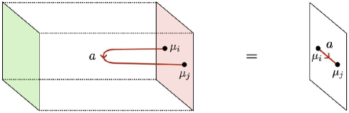
A similar construction of symmetric operators in 1+1D can be found in [70, 66, 107]. We note that the endpoints of an anyon line on the right boundary are not necessarily topological. The patch operator obtained in this way should be labeled by an anyon of the bulk topological order. In addition, the endpoints of the patch operator would carry extra indices corresponding to the internal degrees of freedom of an anyon. For example, as we will see in Sec. IV, the extra indices at the endpoints are associated with the charge of an anyon when the bulk topological order is Kitaev’s quantum double model (i.e., a -gauge theory) and the symmetry in 1+1D is described by a finite group . Extra indices at the endpoints of an anyon line are also observed in more general non-chiral topological orders [95]. Thus, the patch operator obtained as in Fig. 3 should be denoted by , where is a finite interval on which the patch operator acts, is the label of an anyon in the bulk topological order, and and are extra indices at the two ends and respectively. For later convenience, we express a patch operator diagrammatically as follows:
| (12) |
The above arguments suggest that the anyon data of a 2+1D topological order should be encoded in patch operators in 1+1D systems with finite symmetry.
III.2 Symmetric transparent connectable patch operators
Although we argued that anyons in 2+1D topological orders give rise to patch operators in 1+1D, the converse is not true in general: there are many patch operators that have nothing to do with anyons in the bulk. Therefore, in order to reconstruct the anyon data of 2+1D topological orders from 1+1D systems with finite symmetry, we need to identify patch operators that originate from anyons in the bulk. To this end, in this subsection, we study some properties of the patch operators obtained as in Fig. 3 and derive necessary conditions for patch operators to be related to anyons. We will see that the sandwich construction shown in Fig. 3 naturally leads us to the notion of symmetric transparent patch operators that were introduced in [58, 61].
By construction, the patch operator should satisfy the following properties:
Symmetricity.
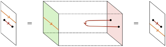
The patch operator is symmetric, i.e., it commutes with the action of fusion category symmetry in 1+1D. This is an immediate consequence of the fact that the symmetry action in 1+1D is implemented by topological lines on the left (i.e., topological) boundary of the 2+1D bulk. Indeed, this definition of the symmetry action guarantees that symmetry operators in 1+1D can freely go through the patch operators obtained as anyon lines attached to the right boundary, see Fig. 4. Thus, the symmetry operators and patch operators commute with each other.
Transparency.
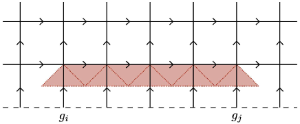
The patch operator is transparent with respect to symmetric operators, i.e., it commutes with any symmetric operators that act non-trivially only in the middle of interval . More specifically, the patch operator can be written as a sum
| (13) |
where on the right-hand side is a (generically non-symmetric) patch operator whose action in the middle of interval is indistinguishable from the symmetry action of an object . The above equation follows from the fact that a bulk anyon line is decomposed into a sum of topological lines when pushed onto a topological boundary as shown in Fig. 5.
When is not contained in the decomposition of , we define . On the other hand, when is contained in the decomposition of multiple times, we have a summation over the multiplicity of on the right-hand side, which is implicit in the above equation. We note that Eq. (13) implies that the patch operator commutes with any symmetric operators whose supports are contained in the middle of interval because the summand does commute with such operators by definition.
When the anyon is condensed on the topological boundary,888An anyon is said to be condensed if its worldline can end topologically on the topological boundary, see [108] for a general theory of anyon condensation. the corresponding patch operator has an empty bulk because condensed anyons become trivial on the boundary. Such a patch operator is called a patch charge operator in [58, 61] because it carries point-like charges at the two ends. The meaning of a charge should be generalized appropriately as in [109, 110] when the symmetry is non-invertible. On the other hand, when the anyon is not condensed on the topological boundary, the corresponding patch operator has a non-empty bulk. Such a patch operator is called a patch symmetry operator in [58, 61] because it looks like a symmetry operator in the middle of the patch.
Connectability.
Patch operators with opposite orientations should be connectable to each other via a “left evaluation” tensor and a “left coevaluation” tensor ,999By abuse of terminology, we will simply call a quantity with indices a tensor in the following. which are represented by the gray ovals in the following equations:
| (14) | |||
where . Here, the orientation-reversal of a patch operator is defined by its Hermitian conjugate:
| (15) |
The summand on the right-hand side of Eq. (15) is denoted by in Eq. (14), i.e., we have
| (16) |
We expect that the orientation-reversal (15) of the patch operator labeled by anyon is equivalent to the patch operator labeled by the dual anyon . Namely, we expect that and differ only by symmetric local operators around the endpoints. For the equivalence of patch operators, see the last paragraph of this subsection. The components and in Eq. (14) may be non-trivial symmetric local operators around the gray ovals, although they are complex numbers in the examples that we will discuss in Sec. IV. For consistency of the diagrammatic representations, we impose the condition that the evaluation and coevaluation tensors are related to their Hermitian conjugates as follows:
| (17) |
This condition guarantees that the Hermitian conjugates of the right-hand sides of Eq. (14) are represented by the diagrams turned upside down and oriented in the opposite direction. The evaluation and coevaluation tensors should satisfy the following zigzag identities:
| (18) | ||||
We note that the second equality automatically follows from the first equality and Eq. (17). There are also a “right evaluation” tensor and a “right coevaluation” tensor , which are represented by the gray ovals in the following equations:
These tensors should also satisfy the zigzag identities analogous to Eq. (18).
The three properties listed above would automatically hold if the patch operator originates from an anyon line of the bulk topological order as shown in Fig. 3. Therefore, these properties are necessary conditions for patch operators to be related to anyons. The importance of these properties was already noticed in [58, 61], where the patch operators with these properties were utilized to reconstruct the anyon data of several topological orders only with abelian anyons. Here, we slightly extended the formulation in [58, 61] so that we can handle more general 2+1D topological orders that may have non-abelian anyons. We emphasize that the explicit form of patch operators with the above properties does not depend on the Hamiltonian of the 1+1D system: it depends only on the symmetry and its representation on the state space.
Based on the above discussion, we conjecture that the anyon data of a 2+1D non-chiral topological order is encoded in the set of symmetric transparent connectable patch operators in 1+1D. More specifically, we conjecture that any topological invariants of a 2+1D topological order described by the Drinfeld center of a fusion category can be computed from symmetric transparent connectable patch operators in 1+1D systems with symmetry . A general computational scheme will be presented in the next subsection.
Before proceeding, we notice that symmetric transparent connectable patch operators have ambiguities around the endpoints because we can multiply symmetric local operators around the endpoints without violating the symmetricity, transparency, and connectability. However, the multiplication by symmetric local operators would not affect the anyon data contained in the patch operators as long as they remain to be symmetric, transparent, and connectable. Therefore, two patch operators should be considered to be equivalent to each other if they differ only by local symmetric operators around the endpoints. We expect that equivalence classes of symmetric transparent connectable patch operators are sufficient to reconstruct the anyon data of 2+1D topological orders.
III.3 General Scheme to compute topological invariants
In this subsection, we propose a general scheme to compute topological invariants of 2+1D topological orders by using symmetric transparent connectable patch operators in 1+1D. To this end, we first introduce twisted evaluation and coevaluation tensors, which allow us to connect two patch operators in the presence of another patch operator in between. Pictorially, the twisted evaluation tensor and the twisted coevaluation tensor are expressed as follows:
where . The components and are supposed to be symmetric local operators. In particular, they commute with in the above equations. When the patch operator inserted in between is oriented in the opposite direction, we use the Hermitian conjugates of and to connect two patch operators. Similarly, there also exist twisted versions of the right evaluation and coevaluation tensors, which are expressed diagrammatically as follows:
In the above equations, we should be able to freely move the patch operators inserted in the middle to the top or bottom because these patch operators correspond to anyon lines in the bulk. More specifically, we should impose the following consistency conditions on the twisted evaluation and coevaluation tensors:
| (19) | ||||
We also have the consistency conditions obtained by flipping the diagrams horizontally and/or vertically in the above equations. These consistency conditions are supposed to be satisfied regardless of the orientations of the patch operators. Equation (19) can be expressed more explicitly in terms of , , and . For example, the first equality in Eq. (19) can be written as
where we chose specific orientations of the patch operators for concreteness. The other two conditions in Eq. (19) can also be expressed in a similar manner.
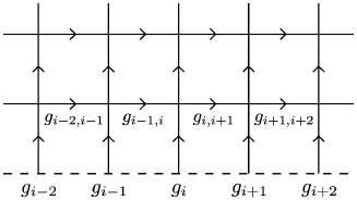
Now, we propose a general method to compute topological invariants of 2+1D topological orders by using symmetric transparent connectable patch operators and twisted evaluation/coevaluation tensors. Our computational scheme goes as follows (see also Fig. 6 for an illustrative example):
-
1.
First, we draw a closed anyon diagram on a two-dimensional plane.
-
2.
We then continuously deform the anyon diagram so that it consists only of horizontal lines and vertical lines. As a convention, we require that a horizontal line is always above a vertical line when they intersect each other. The reason for adopting this convention will be explained shortly.
-
3.
Finally, we translate the anyon diagram into a product of patch operators whose indices at the endpoints are contracted by using the twisted evaluation and coevaluation tensors. Here, horizontal lines of an anyon diagram correspond to patch operators, while vertical lines correspond to twisted evaluation and coevaluation tensors.
The idea of identifying an anyon diagram with a contracted product of patch operators would be justified by the relation between anyon lines and patch operators illustrated in Fig. 3. The convention adopted in the second step is due to the fact that the 1+1D system obtained as in Fig. 3 is viewed from the left side of the 2+1D bulk as we mentioned in Sec. III.1. Indeed, if we view the system from the left side of the bulk, anyon lines are always in front of twisted evaluation and coevaluation tensors living on the right boundary. Thus, the third step of the above prescription makes sense only when the horizontal lines of an anyon diagram are above vertical lines when they intersect.
The above computational scheme would be valid for any topological invariants associated with framed knots and links of anyon lines in 2+1D. In particular, the result of a computation should be invariant under continuous deformations of the anyon diagram due to the defining properties of the patch operators and the consistency conditions on the twisted evaluation/coevaluation tensors. We conjecture that the above prescription enables us to reconstruct the Drinfeld center of a fusion category from symmetric transparent connectable patch operators in 1+1D systems with symmetry .101010If we adopt the convention that horizontal lines are below vertical lines in the second step of the prescription, we end up with the reverse category , which is equivalent to the Drinfeld center of the opposite category [86]. This is consistent with the fact that the symmetry of the 1+1D system becomes if we view the system from the right side of the 2+1D bulk. In the subsequent section, we will see that the above method does work in the case of Kitaev’s quantum double topological order for general finite group .
Let us write down explicit formulae for several topological invariants in terms of patch operators.
Quantum dimension.
Since the quantum dimension is the topological invariant associated with a loop of an anyon line, it can be computed as the contracted product of two patch operators oriented in opposite directions:
| (20) |
More concretely, the quantum dimension can be expressed as
Topological spin.
The topological spin is the topological invariant associated with an anyon line forming a figure of eight. This can be computed as a contracted product of four patch operators labeled by the same anyon:
| (21) |
Modular -matrix.
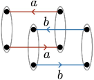
The modular -matrix is the topological invariant associated with the Hopf link. As shown in Fig. 6, it can be computed as a contracted product of four patch operators:
| (22) |
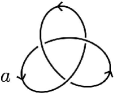
Trefoil knot.
The trefoil knot is a non-trivial knot shown in Fig. 7a. The associated topological invariant, which we denote by , can be computed as a contracted product of six patch operators as follows:111111The authors thank Arkya Chatterjee and Nathanan Tantivasadakarn for discussions on the derivation of equations (23) and (24).
| (23) |
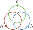
Borromean rings.
The Borromean rings shown in Fig. 7b consist of three linking loops, any two of which are not linked together. The associated topological invariant can be computed as a contracted product of 10 patch operators as follows:
| (24) |
We note that is an example of a topological invariant beyond modular data [89].
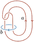
Whitehead link
The Whitehead link is a framed link consisting of two components as shown in Fig. 7c. The associated topological invariant can be computed as a contracted product of 10 patch operators as follows:
| (25) |
The matrix whose -component is given by is called the -matrix and is shown to be beyond modular data [88]
The product of patch operators with boundary indices being contracted as in the above equations gives rise to a complex number on the entire state space of the 1+1D system. This is because an operator defined by the contracted product of patch operators can be shifted freely to the left and right by using the zigzag identities like Eq. (18), which implies that this operator is proportional to the identity operator. This is in contrast to the fact that a similar computation based on ribbon operators in 2+1D results in the correct topological invariants only on the ground state subspace of the topological order.
IV Reconstruction of Kitaev’s quantum double topological order
In this section, based on the general scheme presented in Sec. III.3, we compute the anyon data of Kitaev’s quantum double model from symmetric transparent connectable patch operators in 1+1D systems with non-anomalous finite group symmetry .
IV.1 Patch operators for symmetry and the toric code model
As the simplest example, we begin with the case where . In this case, Kitaev’s quantum double model reduces to the toric code model [98]. The computation of the anyon data of the toric code was discussed in detail in [58, 61] from the point of view of patch operators in 1+1 dimensions. Here, we review this computation with an eye toward a generalization to the case of a general finite group .
We first write down patch operators of 1+1D systems with symmetry. To this end, we need to specify the state space on which the patch operators act. For simplicity, we suppose that the total Hilbert space is given by the tensor product of two-dimensional on-site Hilbert spaces, i.e., we have where denotes a site of a one-dimensional lattice and is the state space on site . In other words, we consider a one-dimensional chain of qubits. The symmetry operator for the symmetry is defined by the product of the Pauli operators: . In this situation, we can find the following four patch operators that satisfy the symmetricity, transparency, and connectability conditions [58, 61]:
| (26) | ||||
where is the Pauli operator acting on site . The existence of the above four patch operators is consistent with the fact that the toric code model has four anyon types , and .121212In the notation in Sec. II.2, we can write , where and are the unit element and the generator of , is the trivial representation of , and is the sign representation of . We note that the above patch operators are written in the form of Eq. (13) where the summand on the right-hand side is unique and does not have extra indices at the endpoints of a patch. The twisted evaluation and coevaluation tensors for these patch operators are trivial, i.e., we have
| (27) |
for all anyon types .
Following the prescription given in Sec. III.3, we can compute the anyon data of the toric code model from the above patch operators. For example, the quantum dimension of an anyon is computed as the contracted product of two patch operators and as in Eq. (20). Since the evaluation and coevaluation tensors (27) are trivial, the contracted product reduces to the ordinary product of and , which is equal to one because in Eq. (26) is unitary for all :
| (28) |
This result agrees with the fact that the anyons of the toric code model are all abelian. Similarly, the topological spins (21) and modular -matrix (22) can be computed as
where . These agree with the correct values of the topological spins and modular -matrix of the toric code anyons [98].
IV.2 Patch operators for symmetry and the quantum double model
We generalize the above computation to the case of a general finite group . To this end, we first write down patch operators in 1+1D systems with finite group symmetry . For simplicity, we suppose that the state space of the system is given by the tensor product , where the on-site Hilbert space is the regular representation of . Namely, the basis states on every site are labeled by group elements of , and the symmetry acts on them by the left multiplication. Specifically, the symmetry operator for is given by the tensor product of on-site operators defined by for all . In this situation, we can find symmetric transparent connectable patch operators labeled by pairs , where is the conjugacy class of and is a unitary irreducible representation of the centralizer . The patch operator labeled by can be explicitly written as
| (29) |
Here, is the symmetry operator acting only on interval , i.e., . On the other hand, the operator is a charge operator that acts only on the endpoints of interval . More specifically, the action of on a basis state is given by
where for is an arbitrary element of that satisfies . The right-hand side of the above equation makes sense because the product is always in the centralizer of . We note that and commute with each other. The twisted evaluation and coevaluation tensors for the patch operators (29) are given by
| (30) | ||||
where , , and denotes the Kronecker delta. As we will see in Appendix A, the patch operators (29) can also be obtained as ribbon operators on the rough boundary of Kitaev’s quantum double model.
When is abelian, the patch operator (29) can be written as , where is the on-site charge operator defined by for all . In particular, when , equation (29) reduces to the patch operators (26) that we wrote down in the previous subsection.
The above expression of the patch operators allows us to explicitly compute various topological invariants following the general scheme presented in Sec. III.3. First of all, the quantum dimension of an anyon labeled by a pair can be computed as
| (31) |
where denotes the summand on the right-hand side of Eq. (29), and is its complex conjugate. We note that Eq. (31) agrees with the correct quantum dimension (9) of an anyon labeled by . Similarly, we can compute the topological spins and modular -matrix by taking the contracted products of four patch operators as in Eqs. (21) and (22):
| (32) |
| (33) | ||||
where . These agree with the correct topological spins (10) and modular -matrix (11) of Kitaev’s quantum double topological order that we reviewed in Sec. II.2. Equations (32) and (33) can be derived by directly computing the action of the contracted product of the patch operators on an arbitrary basis state of the state space . In the derivation of Eq. (33), we used the fact that and are related by the equality
| (34) |
We can also compute other topological invariants such as those associated with the trefoil knot , the Borromean rings , and the Whitehead link . Direct computation based on the formulae (23), (24), and (25) shows
| (35) |
| (36) |
| (37) |
where is the commutation relation between and , which is equal to the unit element if and only if and commute with each other. The summation on the right-hand side of Eq. (36) is taken over group elements , , and that satisfy the following commutation relations:
| (38) |
Similarly, the summation on the right-hand side of Eq. (37) is taken over group elements and that satisfy
| (39) |
The second equality of Eq. (35) follows from the relation , which is an immediate consequence of Eq. (32) and Schur’s lemma. In the derivation of Eqs. (36) and (37), we again used Eq. (34). We note that is unity when is abelian. The topological invariant was also computed by a different method in [90].
V Discussion
In this paper, we proposed a general method to reconstruct the data of topological orders in 2+1 dimensions from symmetric transparent connectable patch operators in 1+1D systems with finite symmetries. Our proposal is based on the observation that anyons in 2+1D topological orders are related to symmetric transparent connectable patch operators in 1+1 dimensions via the sandwich construction as illustrated in Fig. 3. We demonstrated the validity of our proposal by explicitly computing the anyon data of Kitaev’s quantum double topological order from patch operators of 1+1D systems with general finite group symmetry. This result supports the conjecture in [61] that the algebra of symmetric transparent patch operators determines a topological order in one higher dimension.
As an application of patch operators, we expect that the symmetric transparent connectable patch operators that we discussed in this paper would serve as order and disorder operators for gapped phases with finite symmetries. Specifically, the expectation value of a patch operator in the symmetric ground state would remain non-zero in the limit if the anyon is condensed on the right boundary of the 2+1D bulk in Fig. 3, whereas it would go to zero in the limit if the anyon is not condensed on the right boundary. Thus, the expectation values of these patch operators would tell us which anyons are condensed and which are not. This enables us to distinguish different gapped phases corresponding to different sets of condensed anyons on the right boundary. Order and disorder operators are studied from this point of view in, e.g., [58, 43, 111, 70, 66, 107], see also [112, 113] for a general framework. It would be interesting to see whether symmetric transparent connectable patch operators (29) really serve as order and disorder operators in concrete lattice models with finite group symmetry . When is abelian, it was shown in [114] that all gapped phases are distinguished by the set of expectation values of the extended operators of the form (29).
A natural generalization of our study is to incorporate anomalies of finite group symmetries in 1+1D. When finite group symmetries are anomalous, the corresponding 2+1D topological orders are those realized by the twisted quantum double model [100]. It would be interesting to figure out symmetric transparent connectable patch operators in this case and reconstruct the twisted quantum double topological orders from them. More generally, one can consider the case of more general fusion category symmetries [39, 40, 41], where it might be convenient to use matrix product operators in [73, 74] to represent patch operators and compute the anyon data of the corresponding topological orders. Another interesting direction is to generalize our analysis to higher dimensions, where concrete descriptions of topological orders are less understood.
Acknowledgements.
We would like to thank Arkya Chatterjee and Nathanan Tantivasadakarn for helpful discussions. We are grateful to the hospitality of the California Institute of Technology where this work was initiated. K.I. is supported by FoPM, WINGS Program, the University of Tokyo, and by JSPS Research Fellowship for Young Scientists. X.-G.W. was partially supported by NSF grant DMR-2022428 and by the Simons Collaboration on Ultra-Quantum Matter, which is a grant from the Simons Foundation (651446, XGW).Appendix A Ribbon operators on the rough boundary of Kitaev’s quantum double model
In this appendix, we briefly review ribbon operators of Kitaev’s quantum double model following [115, 116]. In particular, we will see a relation between the ribbon operators on the rough boundary of Kitaev’s quantum double model and the patch operators (29) of 1+1D systems with finite group symmetry .
We consider Kitaev’s quantum double model on a square lattice with a rough boundary. Edges of the square lattice are oriented as shown in Fig. 8a.
The state space on each edge is spanned by group elements of . The Hamiltonian of the model is given by
| (40) |
where the vertex term and the plaquette term are defined as follows [98]:
| (41) |
| (42) |
We note that the plaquette terms on the rough boundary constrain the configuration of dynamical variables in Fig. 8a so that for all boundary edges.
Taking the above constraint into account, we can compute the action of a ribbon operator on an interval on the rough boundary as [115, 116]
| (43) | ||||
where , is a basis state on the rough boundary (see Fig. 8a), and for every site on interval . As in the main text, and denote the conjugacy class and centralizer of respectively, is a unitary irreducible representation of , and is an arbitrary element of that satisfies for . The above ribbon operator is illustrated in Fig. 8b. The right-hand side of Eq. (43) is non-zero only when is in the centralizer of . This condition is satisfied if and only if . Therefore, Eq. (43) reduces to
| (44) | ||||
Summing up the above ribbon operators for all leads to
| (45) | ||||
where is the patch operator (29) of 1+1D systems with finite group symmetry . This equation shows the relation between ribbon operators of 2+1D Kitaev’s quantum double model and symmetric transparent connectable patch operators in 1+1 dimensions.
References
- Wen [1990] X.-G. Wen, Topological Order in Rigid States, Int. J. Mod. Phys. B 4, 239 (1990).
- Zeng and Wen [2015] B. Zeng and X.-G. Wen, Gapped quantum liquids and topological order, stochastic local transformations and emergence of unitarity, Phys. Rev. B 91, 125121 (2015), arXiv:1406.5090 .
- Swingle and McGreevy [2016] B. Swingle and J. McGreevy, Renormalization group constructions of topological quantum liquids and beyond, Phys. Rev. B 93, 045127 (2016), arXiv:1407.8203 .
- Atiyah [1988] M. Atiyah, Topological quantum field theories, Publications Mathématiques de l’Institut des Hautes Études Scientifiques 68, 175 (1988).
- Witten [1989] E. Witten, Quantum Field Theory and the Jones Polynomial, Commun. Math. Phys. 121, 351 (1989).
- Kong and Wen [2014a] L. Kong and X.-G. Wen, Braided fusion categories, gravitational anomalies, and the mathematical framework for topological orders in any dimensions (2014a), arXiv:1405.5858 [cond-mat.str-el] .
- Leinaas and Myrheim [1977] J. M. Leinaas and J. Myrheim, On the theory of identical particles, Nuovo Cim B 37, 1 (1977).
- Wilczek [1982] F. Wilczek, Quantum mechanics of fractional-spin particles, Phys. Rev. Lett. 49, 957 (1982).
- Halperin [1984] B. I. Halperin, Statistics of quasiparticles and the hierarchy of fractional quantized Hall states, Phys. Rev. Lett. 52, 1583 (1984).
- Arovas et al. [1984] D. Arovas, J. R. Schrieffer, and F. Wilczek, Fractional statistics and the quantum Hall effect, Phys. Rev. Lett. 53, 722 (1984).
- Wu [1984] Y.-S. Wu, General theory for quantum statistics in two dimensions, Phys. Rev. Lett. 52, 2103 (1984).
- Moore and Seiberg [1989a] G. Moore and N. Seiberg, Classical and quantum conformal field theory, Commun.Math. Phys. 123, 177 (1989a).
- Wen [2016] X.-G. Wen, A theory of 2+1D bosonic topological orders, Natl. Sci. Rev. 3, 68 (2016), arXiv:1506.05768 [cond-mat.str-el] .
- Kitaev [2006] A. Kitaev, Anyons in an exactly solved model and beyond, Annals Phys. 321, 2 (2006), arXiv:cond-mat/0506438 .
- Lan et al. [2018] T. Lan, L. Kong, and X.-G. Wen, Classification of (3+1)D bosonic topological orders: the case when pointlike excitations are all bosons, Phys. Rev. X 8, 021074 (2018), arXiv:1704.04221 .
- Lan and Wen [2019] T. Lan and X.-G. Wen, Classification of 3+1D bosonic topological orders (II): the case when some pointlike excitations are fermions, Phys. Rev. X 9, 021005 (2019), arXiv:1801.08530 .
- Johnson-Freyd [2022] T. Johnson-Freyd, On the Classification of Topological Orders, Commun. Math. Phys. 393, 989 (2022), arXiv:2003.06663 [math.CT] .
- Kong and Zheng [2022] L. Kong and H. Zheng, Categories of quantum liquids I, J. High Energ. Phys. 2022 (8), 1, arXiv:2011.02859 .
- Chatterjee et al. [2022] A. Chatterjee, W. Ji, and X.-G. Wen, Emergent maximal categorical symmetry in a gapless state (2022), arXiv:2212.14432 [cond-mat.str-el] .
- ’t Hooft [1980] G. ’t Hooft, Naturalness, chiral symmetry, and spontaneous chiral symmetry breaking, in Recent Developments in Gauge Theories. NATO Advanced Study Institutes Series (Series B. Physics), Vol. 59, edited by G. ’t Hooft et al. (Springer, Boston, MA., 1980) pp. 135–157.
- Nussinov and Ortiz [2009a] Z. Nussinov and G. Ortiz, Sufficient symmetry conditions for topological quantum order, Proc. Natl. Acad. Sci. U.S.A. 106, 16944 (2009a), arXiv:cond-mat/0605316 .
- Nussinov and Ortiz [2009b] Z. Nussinov and G. Ortiz, A symmetry principle for topological quantum order, Ann. Phys. 324, 977 (2009b), arXiv:cond-mat/0702377 .
- Gaiotto et al. [2015] D. Gaiotto, A. Kapustin, N. Seiberg, and B. Willett, Generalized global symmetries, Journal of High Energy Physics 02, 172 (2015), arXiv:1412.5148 [hep-th] .
- Kapustin and Thorngren [2013] A. Kapustin and R. Thorngren, Higher symmetry and gapped phases of gauge theories (2013), arXiv:1309.4721 [hep-th] .
- Barkeshli et al. [2019] M. Barkeshli, P. Bonderson, M. Cheng, and Z. Wang, Symmetry Fractionalization, Defects, and Gauging of Topological Phases, Phys. Rev. B 100, 115147 (2019), arXiv:1410.4540 [cond-mat.str-el] .
- Córdova et al. [2019] C. Córdova, T. T. Dumitrescu, and K. Intriligator, Exploring 2-group global symmetries, Journal of High Energy Physics 2019, 184 (2019), arXiv:1802.04790 [hep-th] .
- Benini et al. [2019] F. Benini, C. Córdova, and P.-S. Hsin, On 2-group global symmetries and their anomalies, Journal of High Energy Physics 03, 118 (2019), arXiv:1803.09336 [hep-th] .
- Verlinde [1988] E. P. Verlinde, Fusion Rules and Modular Transformations in 2D Conformal Field Theory, Nucl. Phys. B 300, 360 (1988).
- Petkova and Zuber [2001] V. B. Petkova and J. B. Zuber, Generalized twisted partition functions, Phys. Lett. B 504, 157 (2001), arXiv:hep-th/0011021 .
- Fuchs et al. [2002] J. Fuchs, I. Runkel, and C. Schweigert, TFT construction of RCFT correlators I: Partition functions, Nucl. Phys. B 646, 353 (2002), arXiv:hep-th/0204148 .
- Fröhlich et al. [2004] J. Fröhlich, J. Fuchs, I. Runkel, and C. Schweigert, Kramers-Wannier duality from conformal defects, Phys. Rev. Lett. 93, 070601 (2004), arXiv:cond-mat/0404051 .
- Fröhlich et al. [2007] J. Fröhlich, J. Fuchs, I. Runkel, and C. Schweigert, Duality and defects in rational conformal field theory, Nucl. Phys. B 763, 354 (2007), arXiv:hep-th/0607247 .
- Fuchs et al. [2007] J. Fuchs, M. R. Gaberdiel, I. Runkel, and C. Schweigert, Topological defects for the free boson CFT, J. Phys. A 40, 11403 (2007), arXiv:0705.3129 [hep-th] .
- Fröhlich et al. [2009] J. Fröhlich, J. Fuchs, I. Runkel, and C. Schweigert, Defect lines, dualities, and generalised orbifolds, in 16th International Congress on Mathematical Physics (2009) arXiv:0909.5013 [math-ph] .
- Davydov et al. [2011] A. Davydov, L. Kong, and I. Runkel, Field theories with defects and the centre functor, in Mathematical Foundations of Quantum Field Theory and Perturbative String Theory, Proceedings of Symposia in Pure Mathematics, Vol. 83, edited by H. Sati and U. Schreiber (American Mathematical Society, Providence, RI, 2011) pp. 71–128, arXiv:1107.0495 [math.QA] .
- Carqueville and Runkel [2016] N. Carqueville and I. Runkel, Orbifold completion of defect bicategories, Quantum Topol. 7, 203 (2016), arXiv:1210.6363 [math.QA] .
- Brunner et al. [2014] I. Brunner, N. Carqueville, and D. Plencner, Orbifolds and topological defects, Commun. Math. Phys. 332, 669 (2014), arXiv:1307.3141 [hep-th] .
- Brunner et al. [2015] I. Brunner, N. Carqueville, and D. Plencner, Discrete torsion defects, Commun. Math. Phys. 337, 429 (2015), arXiv:1404.7497 [hep-th] .
- Bhardwaj and Tachikawa [2018] L. Bhardwaj and Y. Tachikawa, On finite symmetries and their gauging in two dimensions, Journal of High Energy Physics 03, 189 (2018), arXiv:1704.02330 [hep-th] .
- Chang et al. [2019] C.-M. Chang, Y.-H. Lin, S.-H. Shao, Y. Wang, and X. Yin, Topological defect lines and renormalization group flows in two dimensions, Journal of High Energy Physics 01, 26 (2019), arXiv:1802.04445 [hep-th] .
- Thorngren and Wang [2019] R. Thorngren and Y. Wang, Fusion Category Symmetry I: Anomaly In-Flow and Gapped Phases (2019), arXiv:1912.02817 [hep-th] .
- Kong et al. [2020] L. Kong, T. Lan, X.-G. Wen, Z.-H. Zhang, and H. Zheng, Classification of topological phases with finite internal symmetries in all dimensions, J. High Energ. Phys. 2020 (9), 93, arXiv:2003.08898 .
- Kong et al. [2020] L. Kong, T. Lan, X.-G. Wen, Z.-H. Zhang, and H. Zheng, Algebraic higher symmetry and categorical symmetry – a holographic and entanglement view of symmetry, Phys. Rev. Res. 2, 043086 (2020), arXiv:2005.14178 [cond-mat.str-el] .
- Freed et al. [2022] D. S. Freed, G. W. Moore, and C. Teleman, Topological symmetry in quantum field theory (2022), arXiv:2209.07471 [hep-th] .
- Choi et al. [2022] Y. Choi, C. Córdova, P.-S. Hsin, H. T. Lam, and S.-H. Shao, Noninvertible duality defects in 3+1 dimensions, Phys. Rev. D 105, 125016 (2022), arXiv:2111.01139 [hep-th] .
- Kaidi et al. [2022] J. Kaidi, K. Ohmori, and Y. Zheng, Kramers-Wannier-like Duality Defects in (3+1)D Gauge Theories, Phys. Rev. Lett. 128, 111601 (2022), arXiv:2111.01141 [hep-th] .
- McGreevy [2023] J. McGreevy, Generalized Symmetries in Condensed Matter, Annual Review of Condensed Matter Physics 14, 57 (2023), arXiv:2204.03045 [cond-mat.str-el] .
- Córdova et al. [2022] C. Córdova, T. T. Dumitrescu, K. Intriligator, and S.-H. Shao, Snowmass White Paper: Generalized Symmetries in Quantum Field Theory and Beyond, in Snowmass 2021 (2022) arXiv:2205.09545 [hep-th] .
- Schäfer-Nameki [2023] S. Schäfer-Nameki, ICTP Lectures on (Non-)Invertible Generalized Symmetries (2023), arXiv:2305.18296 [hep-th] .
- Brennan and Hong [2023] T. D. Brennan and S. Hong, Introduction to Generalized Global Symmetries in QFT and Particle Physics (2023), arXiv:2306.00912 [hep-ph] .
- Shao [2023] S.-H. Shao, What’s Done Cannot Be Undone: TASI Lectures on Non-Invertible Symmetry (2023), arXiv:2308.00747 [hep-th] .
- Kong and Wen [2014b] L. Kong and X.-G. Wen, Braided fusion categories, gravitational anomalies, and the mathematical framework for topological orders in any dimensions, (2014b), arXiv:1405.5858 .
- Fiorenza and Valentino [2015] D. Fiorenza and A. Valentino, Boundary conditions for topological quantum field theories, anomalies and projective modular functors, Commun. Math. Phys. 338, 1043 (2015), arXiv:1409.5723 .
- Monnier [2015] S. Monnier, Hamiltonian anomalies from extended field theories, Commun. Math. Phys. 338, 1327 (2015), arXiv:1410.7442 .
- Kong et al. [2015a] L. Kong, X.-G. Wen, and H. Zheng, Boundary-bulk relation for topological orders as the functor mapping higher categories to their centers (2015a), arXiv:1502.01690 .
- Kong et al. [2017a] L. Kong, X.-G. Wen, and H. Zheng, Boundary-bulk relation in topological orders, Nucl. Phys. B 922, 62 (2017a), arXiv:1702.00673 .
- Ji and Wen [2019] W. Ji and X.-G. Wen, Non-invertible anomalies and mapping-class-group transformation of anomalous partition functions, Phys. Rev. Research 1, 033054 (2019), arXiv:1905.13279 .
- Ji and Wen [2020] W. Ji and X.-G. Wen, Categorical symmetry and noninvertible anomaly in symmetry-breaking and topological phase transitions, Phys. Rev. Res. 2, 033417 (2020), arXiv:1912.13492 [cond-mat.str-el] .
- Chatterjee et al. [2022] A. Chatterjee, W. Ji, and X.-G. Wen, Emergent generalized symmetry and maximal symmetry-topological-order (2022), arXiv:2212.14432 .
- Freed [2022] D. S. Freed, Introduction to topological symmetry in QFT (2022), arXiv:2212.00195 [hep-th] .
- Chatterjee and Wen [2023a] A. Chatterjee and X.-G. Wen, Symmetry as a shadow of topological order and a derivation of topological holographic principle, Phys. Rev. B 107, 155136 (2023a), arXiv:2203.03596 [cond-mat.str-el] .
- Zhang and Levin [2023] C. Zhang and M. Levin, Exactly Solvable Model for a Deconfined Quantum Critical Point in 1D, Phys. Rev. Lett. 130, 026801 (2023), arXiv:2206.01222 .
- Lichtman et al. [2021] T. Lichtman, R. Thorngren, N. H. Lindner, A. Stern, and E. Berg, Bulk anyons as edge symmetries: Boundary phase diagrams of topologically ordered states, Phys. Rev. B 104, 075141 (2021), arXiv:2003.04328 [cond-mat.str-el] .
- Gaiotto and Kulp [2021] D. Gaiotto and J. Kulp, Orbifold groupoids, Journal of High Energy Physics 02, 132 (2021), arXiv:2008.05960 [hep-th] .
- Aasen et al. [2020] D. Aasen, P. Fendley, and R. S. K. Mong, Topological Defects on the Lattice: Dualities and Degeneracies (2020), arXiv:2008.08598 [cond-mat.stat-mech] .
- Moradi et al. [2022] H. Moradi, S. F. Moosavian, and A. Tiwari, Topological Holography: Towards a Unification of Landau and Beyond-Landau Physics (2022), arXiv:2207.10712 [cond-mat.str-el] .
- Lin et al. [2023] Y.-H. Lin, M. Okada, S. Seifnashri, and Y. Tachikawa, Asymptotic density of states in 2d CFTs with non-invertible symmetries, JHEP 03, 094, arXiv:2208.05495 [hep-th] .
- Lin and Shao [2023] Y.-H. Lin and S.-H. Shao, Bootstrapping noninvertible symmetries, Phys. Rev. D 107, 125025 (2023), arXiv:2302.13900 [hep-th] .
- Zhang and Córdova [2023] C. Zhang and C. Córdova, Anomalies of (1+1)D categorical symmetries (2023), arXiv:2304.01262 [cond-mat.str-el] .
- Freed and Teleman [2022] D. S. Freed and C. Teleman, Topological dualities in the Ising model, Geom. Topol. 26, 1907 (2022), arXiv:1806.00008 [math.AT] .
- Apruzzi et al. [2021] F. Apruzzi, F. Bonetti, I. García Etxebarria, S. S. Hosseini, and S. Schäfer-Nameki, Symmetry TFTs from String Theory (2021), arXiv:2112.02092 [hep-th] .
- Lan and Zhou [2023] T. Lan and J.-R. Zhou, Quantum current and holographic categorical symmetry (2023), arXiv:2305.12917 [cond-mat.str-el] .
- Lootens et al. [2021] L. Lootens, C. Delcamp, G. Ortiz, and F. Verstraete, Dualities in one-dimensional quantum lattice models: symmetric Hamiltonians and matrix product operator intertwiners (2021), arXiv:2112.09091 [quant-ph] .
- Lootens et al. [2022] L. Lootens, C. Delcamp, and F. Verstraete, Dualities in one-dimensional quantum lattice models: topological sectors (2022), arXiv:2211.03777 [quant-ph] .
- Haag [1996] R. Haag, Local Quantum Physics, 2nd ed., Theoretical and Mathematical Physics (Springer Berlin, Heidelberg, 1996).
- Doplicher et al. [1969a] S. Doplicher, R. Haag, and J. E. Roberts, Fields, observables and gauge transformations I, Commun. Math. Phys. 13, 1 (1969a).
- Doplicher et al. [1969b] S. Doplicher, R. Haag, and J. E. Roberts, Fields, observables and gauge transformations II, Commun. Math. Phys. 15, 173 (1969b).
- Doplicher et al. [1971] S. Doplicher, R. Haag, and J. E. Roberts, Local observables and particle statistics I, Commun. Math. Phys. 23, 199 (1971).
- Doplicher et al. [1974] S. Doplicher, R. Haag, and J. E. Roberts, Local observables and particle statistics II, Commun. Math. Phys. 35, 49 (1974).
- Szlachányi and Vecsernyés [1993] K. Szlachányi and P. Vecsernyés, Quantum symmetry and braid group statistics in -spin models, Commun. Math. Phys. 156, 127 (1993).
- Nill and Szlachányi [1997] F. Nill and K. Szlachányi, Quantum chains of Hopf algebras with quantum double cosymmetry, Commun. Math. Phys. 187, 159 (1997), arXiv:hep-th/9509100 .
- Jones [2023] C. Jones, DHR bimodules of quasi-local algebras and symmetric quantum cellular automata (2023), arXiv:2304.00068 [math-ph] .
- Kong et al. [2022] L. Kong, X.-G. Wen, and H. Zheng, One dimensional gapped quantum phases and enriched fusion categories, Journal of High Energy Physics 03, 22 (2022), arXiv:2108.08835 [cond-mat.str-el] .
- Xu and Zhang [2022] R. Xu and Z.-H. Zhang, Categorical descriptions of 1-dimensional gapped phases with abelian onsite symmetries (2022), arXiv:2205.09656 [cond-mat.str-el] .
- Moore and Seiberg [1989b] G. W. Moore and N. Seiberg, Classical and Quantum Conformal Field Theory, Commun. Math. Phys. 123, 177 (1989b).
- Etingof et al. [2015] P. Etingof, S. Gelaki, D. Nikshych, and V. Ostrik, Tensor Categories, Mathematical Surveys and Monographs, Vol. 205 (American Mathematical Society, Providence, RI, 2015).
- Mignard and Schauenburg [2021] M. Mignard and P. Schauenburg, Modular categories are not determined by their modular data (2021), arXiv:1708.02796 [math.QA] .
- Bonderson et al. [2019] P. Bonderson, C. Delaney, C. Galindo, E. C. Rowell, A. Tran, and Z. Wang, On invariants of Modular categories beyond modular data, J. Pure Appl. Algebra 223, 4065 (2019), arXiv:1805.05736 [math.QA] .
- Delaney and Tran [2018] C. Delaney and A. Tran, A systematic search of knot and link invariants beyond modular data (2018), arXiv:1806.02843 [math.QA] .
- Kulkarni et al. [2021] A. Kulkarni, M. Mignard, and P. Schauenburg, A topological invariant for modular fusion categories (2021), arXiv:1806.03158 [math.QA] .
- Wen and Wen [2019] X. Wen and X.-G. Wen, Distinguish modular categories and 2+1D topological orders beyond modular data: Mapping class group of higher genus manifold (2019), arXiv:1908.10381 [cond-mat.str-el] .
- Delaney et al. [2021] C. Delaney, S. Kim, and J. Plavnik, Zesting produces modular isotopes and explains their topological invariants (2021), arXiv:2107.11374 [math.QA] .
- Fuchs et al. [2013] J. Fuchs, C. Schweigert, and A. Valentino, Bicategories for boundary conditions and for surface defects in 3-d TFT, Commun. Math. Phys. 321, 543 (2013), arXiv:1203.4568 [hep-th] .
- Freed and Teleman [2021] D. S. Freed and C. Teleman, Gapped Boundary Theories in Three Dimensions, Commun. Math. Phys. 388, 845 (2021), arXiv:2006.10200 [math.QA] .
- Levin and Wen [2005] M. A. Levin and X.-G. Wen, String net condensation: A Physical mechanism for topological phases, Phys. Rev. B 71, 045110 (2005), arXiv:cond-mat/0404617 .
- Turaev and Viro [1992] V. G. Turaev and O. Y. Viro, State sum invariants of 3-manifolds and quantum 6j-symbols, Topology 31, 865 (1992).
- Barrett and Westbury [1996] J. W. Barrett and B. W. Westbury, Invariants of piecewise linear three manifolds, Trans. Am. Math. Soc. 348, 3997 (1996), arXiv:hep-th/9311155 .
- Kitaev [2003] A. Y. Kitaev, Fault tolerant quantum computation by anyons, Annals Phys. 303, 2 (2003), arXiv:quant-ph/9707021 .
- Dijkgraaf and Witten [1990] R. Dijkgraaf and E. Witten, Topological Gauge Theories and Group Cohomology, Commun. Math. Phys. 129, 393 (1990).
- Hu et al. [2013] Y. Hu, Y. Wan, and Y.-S. Wu, Twisted quantum double model of topological phases in two dimensions, Phys. Rev. B 87, 125114 (2013), arXiv:1211.3695 [cond-mat.str-el] .
- de Wild Propitius [1995] M. D. F. de Wild Propitius, Topological interactions in broken gauge theories, Ph.D. thesis, Amsterdam U. (1995), arXiv:hep-th/9511195 .
- Kapustin and Saulina [2011] A. Kapustin and N. Saulina, Topological boundary conditions in abelian Chern-Simons theory, Nucl. Phys. B 845, 393 (2011), arXiv:1008.0654 [hep-th] .
- Kitaev and Kong [2012] A. Kitaev and L. Kong, Models for Gapped Boundaries and Domain Walls, Commun. Math. Phys. 313, 351 (2012), arXiv:1104.5047 [cond-mat.str-el] .
- Lan and Wen [2014] T. Lan and X.-G. Wen, Topological quasiparticles and the holographic bulk-edge relation in (2+1)-dimensional string-net models, Phys. Rev. B 90, 115119 (2014), arXiv:1311.1784 [cond-mat.str-el] .
- Kong et al. [2015b] L. Kong, X.-G. Wen, and H. Zheng, Boundary-bulk relation for topological orders as the functor mapping higher categories to their centers (2015b), arXiv:1502.01690 [cond-mat.str-el] .
- Kong et al. [2017b] L. Kong, X.-G. Wen, and H. Zheng, Boundary-bulk relation in topological orders, Nuclear Physics B 922, 62 (2017b), arXiv:1702.00673 [cond-mat.str-el] .
- Albert et al. [2021] V. V. Albert, D. Aasen, W. Xu, W. Ji, J. Alicea, and J. Preskill, Spin chains, defects, and quantum wires for the quantum-double edge (2021), arXiv:2111.12096 [cond-mat.str-el] .
- Kong [2014] L. Kong, Anyon condensation and tensor categories, Nucl. Phys. B 886, 436 (2014), arXiv:1307.8244 [cond-mat.str-el] .
- Bhardwaj and Schäfer-Nameki [2023] L. Bhardwaj and S. Schäfer-Nameki, Generalized Charges, Part II: Non-Invertible Symmetries and the Symmetry TFT (2023), arXiv:2305.17159 [hep-th] .
- Bartsch et al. [2023] T. Bartsch, M. Bullimore, and A. Grigoletto, Representation theory for categorical symmetries (2023), arXiv:2305.17165 [hep-th] .
- Chatterjee and Wen [2023b] A. Chatterjee and X.-G. Wen, Holographic theory for continuous phase transitions: Emergence and symmetry protection of gaplessness, Phys. Rev. B 108, 075105 (2023b), arXiv:2205.06244 [cond-mat.str-el] .
- Bhardwaj et al. [2023a] L. Bhardwaj, L. E. Bottini, D. Pajer, and S. Schafer-Nameki, Gapped Phases with Non-Invertible Symmetries: (1+1)d (2023a), arXiv:2310.03784 [hep-th] .
- Bhardwaj et al. [2023b] L. Bhardwaj, L. E. Bottini, D. Pajer, and S. Schafer-Nameki, Categorical Landau Paradigm for Gapped Phases (2023b), arXiv:2310.03786 [cond-mat.str-el] .
- Else et al. [2013] D. V. Else, S. D. Bartlett, and A. C. Doherty, Hidden symmetry-breaking picture of symmetry-protected topological order, Phys. Rev. B 88, 085114 (2013), arXiv:1304.0783 [cond-mat.str-el] .
- Bombin and Martin-Delgado [2008] H. Bombin and M. A. Martin-Delgado, A Family of Non-Abelian Kitaev Models on a Lattice: Topological Confinement and Condensation, Phys. Rev. B 78, 115421 (2008), arXiv:0712.0190 [cond-mat.str-el] .
- Beigi et al. [2011] S. Beigi, P. W. Shor, and D. Whalen, The Quantum Double Model with Boundary: Condensations and Symmetries, Commun. Math. Phys. 306, 663 (2011), arXiv:1006.5479 [quant-ph] .