LLMLingua: Compressing Prompts for Accelerated Inference
of Large Language Models

Abstract

Large language models (LLMs) have been applied in various applications due to their astonishing capabilities. With advancements in technologies such as chain-of-thought (CoT) prompting and in-context learning (ICL), the prompts fed to LLMs are becoming increasingly lengthy, even exceeding tens of thousands of tokens. To accelerate model inference and reduce cost, this paper presents LLMLingua, a coarse-to-fine prompt compression method that involves a budget controller to maintain semantic integrity under high compression ratios, a token-level iterative compression algorithm to better model the interdependence between compressed contents, and an instruction tuning based method for distribution alignment between language models. We conduct experiments and analysis over four datasets from different scenarios, i.e., GSM8K, BBH, ShareGPT, and Arxiv-March23; showing that the proposed approach yields state-of-the-art performance and allows for up to 20x compression with little performance loss.

1 Introduction

The widespread adoption of ChatGPT has transformed numerous scenarios by harnessing the powerful generalization and reasoning capabilities of large language models (LLMs). In practical applications, crafting suitable prompts is crucial and usually involves techniques such as chain-of-thought, in-context learning, and retrieving related documents or historical conversations Wei et al. (2022); Chase (2022). While these methods can elicit highly effective generations by activating LLMs’ domain-specific knowledge, they often require longer prompts. Therefore, striking a balance between the massive computational demands of LLMs and the need for longer prompts has become an urgent issue. Some studies attempt to accelerate model inference by modifying the parameters of LLMs through quantization Dettmers et al. (2022); Xiao et al. (2023), compression Frantar and Alistarh (2023), etc. However, these approaches may be not suitable when the LLMs can be accessed via APIs only.

Approaches that attempt to reduce the length of original prompts while preserving essential information have emerged lately. These approaches are grounded in the concept that natural language is inherently redundant Shannon (1951) and thus can be compressed. Gilbert et al. (2023) also indicate that LLMs can effectively reconstruct source code from compressed text descriptions while maintaining a high level of functional accuracy. Therefore, we follow this line of studies to compress a long prompt into a shorter one without any gradient flow through the LLMs to support applications based on a larger range of LLMs.

In terms of information entropy, tokens with lower perplexity (PPL) contribute less to the overall entropy gains of the language model. In other words, removing tokens with lower perplexity has a relatively minor impact on the LLM’s comprehension of the context. Motivated by this, Li (2023) propose Selective-Context, which first employs a small language model to compute the self-information of each lexical unit (such as sentences, phrases, or tokens) in original prompts, and then drops the less informative content for prompt compression. However, this method not only ignores the interdependence between the compressed contents but also neglects the correspondence between the LLM being targeted and the small language model used for prompt compression.

This paper proposes LLMLingua, a coarse-to-fine prompt compression method, to address the aforementioned issues. Specifically, we first present a budget controller to dynamically allocate different compression ratios to various components in original prompts such as the instruction, demonstrations, and the question, and meanwhile, perform coarse-grained, demonstration-level compression to maintain semantic integrity under high compression ratios. We further introduce a token-level iterative algorithm for fine-grained prompt compression. Compared with Selective Context, it can better preserve the key information within the prompt by taking into account the conditional dependencies between tokens. Additionally, we pose the challenge of distribution discrepancy between the target LLM and the small language model used for prompt compression, and further propose an instruction tuning based method to align the distribution of both language models.

We validate the effectiveness of our approach on four datasets from different domains, i.e., GSM8K and BBH for reasoning and ICL, ShareGPT for conversation, and Arxiv-March23 for summarization. The results show that our method yields state-of-the-art performance across the board. Furthermore, we conduct extensive experiments and discussions to analyze why our approach attains superior performance. To our best knowledge, we are the first to evaluate reasoning and ICL capabilities in the domain of efficient LLMs.

2 Related Work

2.1 Efficient LLMs

Efficient large language models have gained significant attention in recent research community, especially with the growing prominence of ChatGPT. Most of these methods aim to reduce the costs of inference and fine-tuning by modifying the model parameters through quantization Dettmers et al. (2022); Frantar et al. (2023); Xiao et al. (2023), compression Frantar and Alistarh (2023), instruct tuning Taori et al. (2023); Chiang et al. (2023); Xu et al. (2023), or delta tuning Hu et al. (2022).

A line of studies attempt to optimize inference costs from the perspective of the input prompts. Motivated by the observation of the abundance of identical text spans between the input and the generated result, Yang et al. (2023) directly copy tokens from prompts for decoding to accelerate the inference process of LLMs. Some approaches focus on compressing prompts, specifically, learning special tokens via prompt tuning of LLMs to reduce the number of tokens to be processed during inference Mu et al. (2023); Ge et al. (2022); Wingate et al. (2022); Chevalier et al. (2023); Ge et al. (2023). Unfortunately, these methods are usually tailored to particular tasks and some of them Mu et al. (2023); Chevalier et al. (2023) even require to fine-tune the whole language model, which severely limits their application scenarios. Furthermore, there are some studies Chase (2022); Zhang et al. (2023) that attempt to utilize LLMs to summarize dialog or data, thereby forming memory and knowledge. However, these approaches require multiple invocations of LLMs, which are quite costly.

Some methods reduce the prompt length by selecting a subset of demonstrations. For example, Zhou et al. (2023) introduces a reinforcement learning based algorithm to allocate a specific number of demonstrations for each question. Some other methods focus on token pruning Goyal et al. (2020); Kim and Cho (2021); Kim et al. (2022); Rao et al. (2021); Modarressi et al. (2022) and token merging Bolya et al. (2023). However, these approaches are proposed for smaller models such as BERT, ViT. Moreover, they depend on fine-tuning the models or obtaining intermediate results during inference.

The most similar work to this paper is Selective-Context Li (2023), which evaluates the informativeness of lexical units by computing self-information with a small language model, and drops the less informative content for prompt compression. This paper is inspired by Selective-Context and further proposes a coarse-to-fine framework to address its limitations.

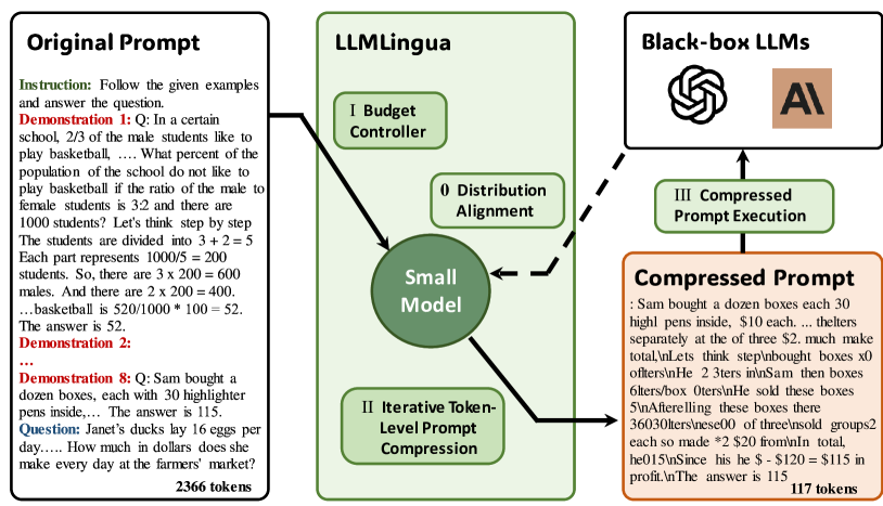
Figure 1: Framework of the proposed approach LLMLingua.

2.2 Out-of-Distribution (OoD) Detection

Recently, a series of studies have been proposed for unsupervised OoD detection. With only in-distribution texts available for learning, these methods either fine-tune a pre-trained language model Arora et al. (2021) or train a language model from scratch Mai et al. (2022). Wu et al. (2023) analyze the characteristics of these methods and leverage multi-level knowledge distillation to integrate their strengths while mitigating their limitations. Finally, perplexity output by the resulting language model is used as the indication of an example being OoD.

This paper also regards perplexity as a measurement of how well a language model predicts a sample. In contrast to out-of-distribution detection, which identifies examples with high perplexities as indicative of unreliable predictions, we consider tokens with higher perplexity to be more influential during the inference process of language models.

2.3 LLMs as a Compressor

Recently, many perspectives have interpreted large language models and unsupervised learning as a kind of compressor for world knowledge Sutskever (2023); Delétang et al. (2023), by using arithmetic coding Rissanen (1976); Pasco (1976). Our research can be viewed as an endeavor to further compress information within prompts by capitalizing on the compression-like characteristics of large language models.

3 Problem Formulation

A prompt compression system is designed to generate a compressed prompt $\widetilde{\bm{x}}=\{\widetilde{x}_{i}\}_{i=1}^{\widetilde{L}}$ from a given original prompt $\bm{x}=(\bm{x}^{\text{ins}},\bm{x}^{\text{dems}},\bm{x}^{\text{que}})$, where $\bm{x}^{\text{ins}}=\{x_{i}^{\text{ins}}\}_{i=1}^{L^{\text{ins}}}$, $\bm{x}^{\text{dems}}=\{x_{i}^{\text{dems}}\}_{i=1}^{L^{\text{dems}}}$, and $\bm{x}^{\text{que}}=\{x_{i}^{\text{que}}\}_{i=1}^{L^{\text{que}}}$ denote the instruction, demonstrations, and the question in the original prompt $\bm{x}$. $\widetilde{L}$, $L_{\text{ins}}$, $L_{\text{dems}}$, and $L_{\text{que}}$ represent the numbers of tokens in $\widetilde{\bm{x}}$, $\bm{x}^{\text{ins}}$, $\bm{x}^{\text{dems}}$, and $\bm{x}^{\text{que}}$, respectively. Let $L=L_{\text{ins}}+L_{\text{dems}}+L_{\text{que}}$ denote the total sequence length of $\bm{x}$, the compression rate is defined as $\tau=\widetilde{L}/L$, $\tau\in[0,1]$, and the compression ratio is $1/\tau$. A smaller value of $\tau$ implies a lower inference cost, which is preferable. Let $\bm{\widetilde{x}}_{G}$ represent the LLM-generated results derived by $\widetilde{\bm{x}}$ and $\bm{x}_{G}$ denotes the tokens derived by $\bm{x}$, the distribution of $\bm{\widetilde{x}}_{G}$ is expected to be as similar to $\bm{x}_{G}$ as possible. This can be formulated as:

$$\min_{\widetilde{\bm{x}},\tau}\text{KL}(P(\widetilde{\bm{x}}_{G}|\widetilde{\bm{x}}),P(\bm{x}_{G}|\bm{x})),$$ (1)

4 Methodology

In this section, we elaborate on the proposed coarse-to-fine prompt compression approach, LLMLingua. First, we introduce a budget controller to dynamically allocate different compression ratios to various components in prompts and meanwhile, perform coarse-grained, demonstration-level compression to maintain semantic integrity under high compression ratios. Next, we describe the proposed iterative prompt algorithm designed to retain knowledge from the prompt while compressing. Finally, we introduce alignment to address the distribution gap between the small model and black-box large models. Figure  1 show the framework.

4.1 Budget Controller

The budget controller here is designed to allocate different budgets, i.e., compression ratio, to different components in a prompt such as instructions, demonstrations, and questions, at the sentence or demonstration level. There are two considerations:

(i) In general, the instruction and the question in a prompt have a direct influence on the generated results, as they should contain all the necessary knowledge to generate the following answer. On the contrary, if there are multiple demonstrations in the original prompt, the conveyed information may be redundant. Therefore, a tailored budget controller is required to allocate more budget (i.e., smaller compression ratios) for instructions and questions, and less budget for demonstrations.

(ii) When a high compression ratio is required, token-level dropout as in Li (2023) might make the compressed prompts too trivial and thus lose vital information from the original prompt. Consequently, sentence-level dropout should be employed instead to preserve a certain degree of linguistic integrity. Especially in the case of multiple redundant demonstrations, we can even perform demonstration-level control to meet the compression requirement.

Algorithm 1 illustrates the overall procedure of the budget controller.

Algorithm 1 Pseudo code of Budget Controller.

Input: A small language model $\mathcal{M}_{s}$; the original prompt $\bm{x}=(\bm{x}^{\text{ins}},\bm{x}^{\text{dems}},\bm{x}^{\text{que}})$.

1:Set the selected demonstration set $\mathcal{D}=\phi$.

2:Get demonstration compression rate $\tau_{\text{dem}}$ by Eq.(2).

3:Calculate the perplexity of each demonstration via $\mathcal{M}_{s}$.

4:Rank all demonstrations in descending order of their perplexity as a list $(\bm{x}^{\text{dem}}_{(1)},...,\bm{x}^{\text{dem}}_{(N)})$, where $N$ is the number of demonstrations, $\bm{x}^{\text{dem}}_{(i)}$ is the $i$-th demonstration.

5:for $i=1$ do

6:     if $\widetilde{L}_{\mathcal{D}}>k\cdot\tau_{\text{dems}}L_{\text{dems}}$ then

7:         Break.

8:     end if

9:     Append $\bm{x}_{(i)}^{\text{dem}}$ to $\mathcal{D}$.

10:     $i=i+1$

11:end for

12:Allocate remaining budget to $\bm{x}^{\text{ins}}$ and $\bm{x}^{\text{que}}$ via Eq. (3).

Output: The subset of demonstrations $\mathcal{D}$ obtained from coarse-grained compression; Additional budget $\Delta\tau_{\text{ins},\text{que}}$ for the instruction and the question.

Derive compression ratio for demonstrations.

We first compute the compression rate for demonstrations $\tau_{\text{dems}}$ according to the target overall compression rate $\tau$ and the pre-defined compression rate for instructions and questions, i.e., $\tau_{\text{ins}}$ and $\tau_{\text{que}}$, respectively.

$$\tau_{\text{dems}}=\frac{\tau L-(\tau_{\text{ins}}L_{\text{ins}}+\tau_{\text{que}}L_{\text{que}})}{L_{\text{dems}}}.$$ (2)

Demonstration-level prompt compression.

With the derived $\tau_{\text{dems}}$ for demonstrations, we then perform a coarse-grained demonstration-level prompt compression: we construct $\mathcal{D}$, a subset of demonstrations from $\bm{x}^{\text{dems}}$.

Specifically, we first employ a small language model $\mathcal{M}_{s}$, such as GPT-2 or LLaMA, to compute the perplexity of each demonstration in $\bm{x}^{\text{dems}}$. Then, we select demonstrations in descending order of their perplexity values, until adding one more demonstration to $\mathcal{D}$ will make the total number of tokens in $\mathcal{D}$ exceed maximum tokens $k\cdot\tau_{\text{dems}}L_{\text{dems}}$, where $k$ is the granular control coefficient.

Adjust compression ratios for instruction and question.

After obtaining the coarse-grained compression result $\mathcal{D}=\{x_{i}\}_{i=1}^{\widetilde{L}_{\mathcal{D}}}$, we allocate the remaining budget to the instruction and the question:

$$\Delta\tau=\frac{k\cdot\tau_{\text{dems}}L_{\text{dems}}-\widetilde{L}_{\mathcal{D}}}{L_{\text{ins}}+L_{\text{que}}},$$ (3)

where $\widetilde{L}_{\mathcal{D}}$ denote the total number of tokens in $\mathcal{D}$.

4.2 Iterative Token-level Prompt Compression

Algorithm 2 Pseudo code of Iterative Token-level Prompt Compression (ITPC).

Input: A small language model $\mathcal{M}_{s}$; the prompt from budget controller $\bm{x}^{\prime}=(\bm{x}^{\text{ins}},\bm{x}^{\mathcal{D}},\bm{x}^{\text{que}})$; target compression rate$\tau$, adjusted compression rate $\triangle\tau_{\text{ins},\text{que}}$.

1:Set the selected token set $\mathcal{T}=\phi$

2:Get segment set $\mathcal{S}$.

3:for $i=1,2,\ldots,m$ do

4:     Get the conditional probabilities $p(\bm{s}_{i})$ via Eq.(5)

5:     Get the compression threshold $\gamma_{i}$ with Eq. (6).

6:     Append the compressed token to $\mathcal{T}$ via Eq.(7).

7:end for

8:Concatenate all tokens in $\mathcal{T}$ as $\bm{\widetilde{x}}$.

Output: The compressed prompt $\bm{\widetilde{x}}$.

Utilizing perplexity for prompt compression encounters the intrinsic limitation, i.e., the independence assumption, similar to the shortcomings of the Mask Language Model Yang et al. (2019) as:

$$p(\bm{\widetilde{x}}) =\prod_{i=1}^{\widetilde{L}}p(\widetilde{x}_{i}|\widetilde{x}_{<i})$$ (4)

$$\approx p(\bm{x}^{\prime})=\prod_{i=1}^{L^{\prime}}p(x_{i}|\widetilde{x}_{<i},\overline{x}_{<i}),$$

where $\bm{x}^{\prime}=(\bm{x}^{\text{ins}},\bm{x}^{\mathcal{D}},\bm{x}^{\text{que}})$ is the original prompt after demonstration-level compression; $\bm{x}^{\mathcal{D}}$ is the concatenation of all demonstrations in $\mathcal{D}$; $\widetilde{x}$ is the final compressed prompt; $\widetilde{x}_{<i}$ and $\overline{x}_{<i}$ denote the preserved and compressed tokens before the $i$-th token $x_{i}$; $L^{\prime}$ and $\widetilde{L}$ denote the numbers of all tokens in $\bm{x}^{\prime}$ and $\widetilde{\bm{x}}$, respectively.

Here we propose an iterative token-level prompt compression (ITPC) algorithm to mitigate the inaccuracy introduced by the conditional independence assumption. Algorithm 2 shows the pseudo codes.

Specifically, we first divide the target prompt $\bm{x}^{\prime}$ into several segments $\mathcal{S}=\{\bm{s}_{1},\bm{s}_{2},...,\bm{s}_{m}\}$. And then, we use the smaller model $\mathcal{M}_{s}$ to obtain the perplexity distribution of all segments. The compressed prompt obtained from each segment is concatenated to the subsequent segment, enabling more accurate estimation of the conditional probability. The corresponding probability estimation function can be formulated as:

$$p(\bm{\widetilde{s}}_{j}) =\prod_{i=1}^{\sum_{k}^{j}\widetilde{L}_{s,k}}p(\widetilde{s}_{j,i}|\widetilde{s}_{j,<i},\bm{\widetilde{s}}_{<j})$$ (5)

$$\approx\prod_{i=1}^{L_{s,j}+\sum_{k}^{j-1}\widetilde{L}_{s,k}}p(s_{j,i}|s_{j,<i},\bm{\widetilde{s}}_{<j}),$$

where $s_{j,i}$ denotes the $i$-th token in the $j$-th segment, $L_{s,j}$ and $\widetilde{L}_{s,j}$ represent the token length of $j$-th original and compressed segment, respectively.

When the conditional probabilities for each segment $p(\bm{s}_{j})$ are obtained, the compression ratio threshold $\gamma_{j}$ w.r.t. $\bm{s}_{j}$ are dynamically calculated based on the PPL distribution and the corresponding compression ratio $\tau_{\bm{s}_{j}}$, where

$$\tau_{\bm{s}_{j}}=\left\{\begin{aligned} \tau_{\text{ins}}+\Delta\tau,&\quad\text{if $\bm{s}_{j}$ from $\bm{x^{\text{ins}}}$},\\ \tau_{\text{dems}},&\quad\text{if $\bm{s}_{j}$ from $\bm{x^{\mathcal{D}}}$},\\ \tau_{\text{que}}+\Delta\tau,&\quad\text{if $\bm{s}_{j}$ from $\bm{x^{\text{que}}}$}.\\ \end{aligned}\right.$$ (6)

Finally, tokens in each $\bm{s}_{j}$ with the PPL greater than $\gamma_{j}$ are retained in the compressed prompt.

$$\bm{\widetilde{s}}_{j}=\{s_{j,i}|p(s_{j,i})>\gamma_{j}\}$$ (7)

4.3 Distribution Alignment

To narrow the gap between the distribution of the LLM and that of the small language model used for prompt compression, here we align the two distributions via instruction tuning.

Specifically, we start from a pre-trained small language model $\mathcal{M}_{s}$ and use the data generated by the LLM to perform instruction tuning on $\mathcal{M}_{s}$. The optimization of $\mathcal{M}_{s}$ can be formulated as:

$$\min_{\bm{\theta}_{s}}\mathbb{E}\left[\frac{1}{N}\sum_{i=1}^{N}\mathcal{L}\left(\mathbf{x}_{i},\mathbf{y}_{i,\text{LLM}};\bm{\theta}_{\mathcal{M}_{s}}\right)\right],$$ (8)

where $\theta_{\mathcal{M}_{s}}$ denotes the parameters of $\mathcal{M}_{s}$, $(\bm{x}_{i},\bm{y}_{i}^{\text{LLM}})$ denotes the pair of instruction $\bm{x}_{i}$ and the LLM generated texts $\bm{y}_{i}^{\text{LLM}}$, $N$ is the number of all examples used for instruction tuning.

5 Experiments

5.1 Settings

Datasets

To comprehensively assess the effectiveness of compressed prompts in retaining LLM abilities, we evaluated their performance across four datasets. For reasoning and in-context learning (ICL), we use GSM8K Cobbe et al. (2021) and BBH Suzgun et al. (2022). As for contextual understanding, we use ShareGPT sha (2023) for conversation and Arxiv-March23 Li (2023) for summarization. It’s worth noting that neither the small LM nor the target LLMs used in this paper have seen any of the evaluation datasets, especially the last two which were newly collected this year. We followed the experimental setup of previous work Fu et al. (2023a); Li (2023) for the usage of these datasets. Please refer to Appendix A.1 for detailed information.

Evaluation

Following Cobbe et al. (2021), Fu et al. (2023a), and Li (2023), we utilize the Exact Match as the evaluation metric for GSM8K and BBH. We use BLEU Papineni et al. (2002), ROUGE Lin (2004), and BERTScore Zhang et al. (2020) as the evaluation metrics for ShareGPT and Arxiv-March23.

Implementation Details

In this paper, we employ the GPT-3.5-Turbo-0301 and the Claude-v1.3 as the target LLMs, which can be accessed via OpenAI and Claude API. To improve the stability of outputs produced by LLMs we apply greedy decoding with a temperature of $0$ across all experiments. The Alpaca dataset Taori et al. (2023) is exclusively employed for aligning small language models with black-box LLMs, and is not utilized in the evaluation process. In our experiments, we utilize either Alpaca-7B or GPT2-Alpaca as the small pre-trained language model $\mathcal{M}_{s}$ for compression. We implement our approach based on PyTorch 1.12.0 and Huggingface’s Transformers. We set the granular control coefficient $k$ to $2$. We use the pre-defined compression rates $\tau_{\text{ins}}=0.85$ and $\tau_{\text{que}}=0.9$ for instructions and questions. The segment size used in the iterative token-level compression is set to $100$.

Methods	ShareGPT							Arxiv-March23
	BLEU	Rouge1	Rouge2	RougeL	BS F1	Tokens	$1/\tau$	BLEU	Rouge1	Rouge2	RougeL	BS F1	Tokens	$1/\tau$
Constraint I	2x constraint							350 tokens constraint
Sentence Selection	28.59	46.11	31.07	37.94	88.64	388	1.5x	22.77	50.1	25.93	33.63	88.21	379	4x
Selective-Context	25.42	46.47	29.09	36.99	88.92	307	1.9x	21.41	51.3	27.94	36.73	89.60	356	4x
Ours	27.36	48.87	30.32	38.55	89.52	304	1.9x	23.15	54.21	32.66	42.74	90.33	345	4x
Constraint II	3x constraint							175 tokens constraint
Sentence Selection	18.94	35.17	18.96	26.75	85.63	255	2.3x	12.41	38.91	14.25	26.72	87.09	229	7x
Selective-Context	15.79	38.42	20.55	28.89	87.12	180	3.3x	12.23	42.47	19.48	29.47	88.16	185	8x
Ours	19.55	40.81	22.68	30.98	87.70	177	3.3x	13.45	44.36	24.86	34.94	89.03	176	9x

Table 1: Performance of different methods under different target compression ratios on the conversation (ShareGPT) and summarization (Arxiv-March23) task.

Methods	GSM8K			BBH
	EM	Tokens	$1/\tau$	EM	Tokens	$1/\tau$
Full-shot	78.85	2,366	-	70.07	774	-
1-shot constraint
1-shot	77.10	422	6x	69.60	284	3x
Selective-Context	53.98	452	5x	54.27	276	3x
GPT4 Generation	71.87	496	5x	27.13	260	3x
Ours	79.08	446	5x	70.11	288	3x
half-shot constraint
Sentence Selection	72.33	230	10x	39.56	175	4x
Selective-Context	52.99	218	11x	54.02	155	5x
GPT4 Generation	68.61	223	11x	27.09	161	5x
Ours	77.41	171	14x	61.60	171	5x
quarter-shot constraint
Sentence Selection	66.67	195	12x	46.00	109	7x
Selective-Context	44.20	157	15x	47.37	108	7x
GPT4 Generation	56.33	188	20x	26.81	101	8x
Ours	77.33	117	20x	56.85	110	7x
zero-shot	48.75†	11	215x	32.32	16	48x
Simple Prompt	74.9	691	3x	-	-	-

Table 2: Performance of different methods under different target compression ratios on the GSM8K mathematical reasoning and Big-bench Hard (BBH) datasets. ^†We also include the instruction of the prompt in zero-shot experiments for a vertical comparison.

Baselines

We consider the following baselines:

• GPT4-Generation: Instruct GPT-4 to compress the original prompt. We used ten sets of instructions here and reported the best results. Appendix C displays the instructions we employed.

• Random Selection: Random select the demonstrations or sentences of the original prompt.

• Selective-Context Li (2023): Use the phrase-level self-information from a small language model to filter out less informative content. We use the same small LM, i.e., Alpaca-7B for a fair comparison.

5.2 Main Results

Table 1 and 2 report the results of our approach alongside those baseline methods on GSM8K, BBH, ShareGPT, and Arxiv-March23. It can be seen that our proposed method consistently outperforms the prior methods by a large margin in almost all experiments.

Specifically, on GSM8K and BBH, the reasoning and in-context learning-related benchmark, our method even achieves slightly higher results than the full-shot approach, while also delivering impressive compression ratios ($1/\tau$) of 5x and 3x respectively, with the 1-shot constraint. This well demonstrates that our compressed prompts effectively retain the reasoning information contained in the original prompt. As the compression ratio increases, i.e., under the half-shot and quarter-shot constraints, the performance experiences a slight decline. For instance, on GSM8K, the EM scores will decrease by 1.44 and 1.52, respectively, despite compression ratios as high as 14x and 20x. On BBH, our approach achieves compression ratios of 5x and 7x with the EM score decreasing by 8.5 and 13.2 points, respectively. In fact, this performance is already quite satisfactory, as it approaches the score of 62.0 achieved by PaLM-540B in half-shot constraint. Our case study reveals that this declined performance on BBH is mainly due to challenging reasoning tasks, such as tracking_shuffled_objects_seven_objects.

Moreover, on ShareGPT and Arxiv-March23, two contextual understanding benchmarks, we can see that our approach achieves acceleration ratios of 9x and 3.3x with a high BERTScore F1, indicating that our approach successfully retains the semantic information of the initial prompts.

5.3 Analysis on Reasoning & ICL Tasks.

Here we analyze the performance of our approach and baseline methods on the difficult reasoning and in-context learning (ICL) benchmarks GSM8K and BBH.

We notice that our approach shows significant performance improvements over the strong baseline Selective-Context under all settings. We conjecture that, as relying on phrase-level self-information, Selective-Context is prone to lose critical reasoning information during the chain-of-thought process. Especially on GSM8K, its performance is lower than ours by 33.10 points at a compression ratio of 20x. The inferior performance of Sentence Selection suggests that it may face similar issues of fragmentary reasoning logic. Surprisingly, though GPT-4 has demonstrated its strong text generation capability, the suboptimal performance on prompt compression indicates that the generated prompts may omit crucial details from the original prompt, particularly reasoning steps.

In addition to the findings mentioned above, the experiments also demonstrate that our method can preserve the ICL capacity of prompts for LLMs. Compared to the zero-shot results, our approach exhibits significant performance improvements of 51.55 and 24.53 even with the largest compression ratios. Notably, on GSM8K, our 20x compressed prompt outperforms the 8-shot 3-step CoT by 2.43, further suggesting that our method can effectively retain the reasoning information.

5.4 Ablation

To validate the contributions of different components in our approach, we introduce five variants of our model for ablation study: i) Ours w/o Iterative Token-level Compression, which performs token-level compression in a single inference rather than iteratively. ii) Ours w/o Budget Controller, which directly employs ITPC with the same compression ratio for all components. iii) Ours w/o Dynamic Compression Ratio, which uses the same compression ratio for all components. iv) Ours w/ Random Selection in Budget Controller, which randomly selects demonstrations or sentences for demonstration-level prompt compression. v) Ours w/o Distribution Alignment, which removes the distribution alignment module of our approach and directly use the pre-trained LLaMA-7B as the small language model. vi) Ours w/ Remove Stop Words, which removes the stop words in original prompts using NLTK. Table 3 shows the results.

	EM	Tokens	$1/\tau$
Ours	79.08	439	5x
- w/o Iterative Token-level Prompt Compression	72.93	453	5x
- w/o Budget Controller	73.62	486	5x
- w/o Dynamic Compression Ratio	77.26	457	5x
- w/ Random Selection in Budget Controller	72.78	477	5x
- w/o Distribution Alignment	78.62	452	5x
- w/ Remove Stop Words	76.27	1,882	1.3x

Table 3: Ablation study on GSM8K in 1-shot constraint.

Comparing Ours with w/o Iterative Token-level Prompt Compression, we observe a significant decline in Exact Match when the conditional dependence between compressed tokens is not considered. We conjecture this variant may lose essential information in the prompt, especially for low-frequency keywords that frequently appear in the given prompt. When comparing Ours with w/o Dynamic Compression Ratio and with w/o Budget Controller, it reveals that different components of the prompt exhibit varying sensitivity. Instructions and questions necessitate a lower compression ratio. To balance the relationship between compression ratio and language integrity, introducing a demonstration or sentence-level filter better preserves sufficient linguistic information, even at higher compression ratios. Ours w/ Random Selection in Budget Controller indicates that selecting sentences or demonstrations based on perplexity can better identify information-rich sentences for target LLMs. Distribution Alignment allows small LMs to generate distributions that more closely resemble those of target LLMs, resulting in a further improvement of 0.56 on GSM8K.

5.5 Discussion

Different Target LLMs

Here we test our method with Claude-v1.3 as the target LLM to demonstrate its generalizability across different black-box LLMs in addition to the GPT series models. Due to the limitation of API cost, we only consider the scenarios with one-shot constraint and half-shot constraint. Similarly, we employe Alpaca-7B as the small language model for the challenges in collecting alignment data. As shown in Table 4, our method can achieve improvements over the simple prompt by 0.8 and 1.7 EM points with compression ratios of 5x and 14x, respectively.

	EM	Tokens	$1/\tau$
Ours in 1-shot constraint	83.51	439	5x
Ours in half-shot constraint	82.61	171	14x
Simple Prompt	81.8	691	3x

Table 4: Ours method on GSM8K using Claude-v1.3.

Different Small LMs

We further test our approach with different small language models: we fine-tune the GPT2-small on the Alpaca dataset and use it as the small LM for our system. As shown in Table 5, the results obtained by Alpaca finetuned GPT2-small are weaker than those obtained by Alpaca-7B with a performance drop of 2.06, 0.99, and 1.06 EM points at different compression ratios. This is due to the significant distribution discrepancy between the small LM and the target LLM. Even with distribution alignment, it is still difficult to directly estimate the target LLM using the distribution from the small language model. Similar observations have been reported in Li (2023). However, benefiting from the proposed budget controller and the iterative token-level prompt compression algorithm, our approach achieves satisfactory results in difficult tasks such as reasoning even with the less powerful GPT2-Small as the small language model.

	EM	Tokens	$1/\tau$
Ours with GPT2 in 1-shot constraint	77.02	447	5x
Ours with GPT2 in half-shot constraint	76.42	173	14x
Ours with GPT2 in quarter-shot constraint	76.27	128	18x

Table 5: Our method on GSM8K with GPT2-Alpaca as the small language model.

The Generation Results of Compressed Prompt

Appendix E displays several compressed prompts along with following generation texts. It is evident that the compressed prompts can still guide the generation of multi-step reasoning outcomes similar to the original ones. In contrast, prompts compressed using Selective-Context exhibit errors in reasoning logic. This highlights the effectiveness of our method in preserving crucial semantic information while retaining reasoning capabilities.

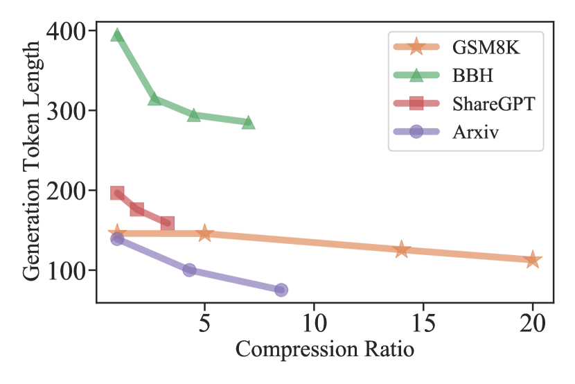
Figure 2: The distribution of generated token lengths at varying compression ratios ($1/\tau$).

As depicted in Figure 2, we also analyze the relationship between the compression ratio and the length of the corresponding generated texts. It can be observed that as the compression ratio increases, the text length produced by target LLMs tends to decrease, albeit with varying degrees across different datasets. This indicates that prompt compression not only saves computational resources in the input but also contributes to computational savings in the generation stage.

Overhead of LLMLingua

We explore two key factors to study the computation overhead of LLMLingua: the number of tokens involved in computation and the end-to-end latency.

The overall computation of our system is the sum of the prompt compression and the following inference. This can be formulated as:

$$c=(L+kL/\tau+L/\tau)\cdot c_{\text{small}}+L/\tau\cdot c_{\text{LLMs}},$$ (9)

where $c_{\text{small}}$ and $c_{\text{LLMs}}$ represent the per token computation load of the small LM and LLM, respectively. $L$, $kL/\tau$, and $L/\tau$ are the numbers of token inferences for the budget controller, the perplexity calculation of tokens to compress in ITPC, and the conditioned perplexity calculation of compressed results in ITPC (using KV cache), respectively. Assuming that the small LM has the same system optimizations as the LLMs, such as the use of FasterTransformer and quantization techniques, we can estimate the ratio between $c_{\text{small}}$ and $c_{\text{LLMs}}$ based on model parameters: $c_{\text{small}}\approx 7/175c_{\text{LLMs}}=1/25c_{\text{LLMs}}$. When $\tau=5$, we have $c\approx 0.264\cdot Lc_{\text{LLMs}}\approx 1/4\cdot Lc_{\text{LLMs}}$. That is, we can achieve nearly 4x savings in computational resources when using the smaller LM with a prompt compression rate of 5x.

$1/\tau$	1x	2x	5x	10x
End-to-End w/o LLMLingua	8.6	-	-	-
End-to-End w/ LLMLingua	-	4.9(1.7x)	2.3(3.3x)	1.3(5.7x)
LLMLingua	-	0.8	0.3	0.2

Table 6: Latency (s) comparison on GSM8K.

Table 6 shows the end-to-end latency of different systems on a V100-32G GPU with a compression rate from 1x to 10x. We can see that LLMLingua has a relatively small computation overhead and can achieve a speedup ranging from 1.7x to 5.7x.

Recovering the Compressed Prompt using LLMs

Appendix D shows some examples restored from the compressed prompts by using GPT-4. It is evident that LLMs can effectively comprehend the semantic information in the compressed prompts, even if it might be challenging for humans. Additionally, we notice that how much information GPT-4 can recover depends on the compression ratio and the small language model we use. For instance, in Figure 4, the prompt compressed using Alpaca-7B is restored to its complete 9-step reasoning process, while in Figure 6, the prompt compressed with GPT2-Alpaca can only be restored to a 7-step reasoning process, with some calculation errors.

Compare with Generation-based Methods

We do not develop our approach based on LLM generation primarily for three reasons: i) The content and length of the generated text are uncontrollable. Uncontrollable length requires more iterations to satisfy the constraint of the compression ratio. Uncontrollable content leads to low overlap between the generated text and the original prompt, particularly for complex prompts with multi-step inference, which may lose significant amounts of reasoning paths or even generate completely unrelated demonstrations. ii) The computational cost is high. Small language models struggle to handle such complex tasks, and using models like GPT-4 for compression would further increase computational overhead. Moreover, even powerful generation models like GPT-4 struggle to retain effective information from prompts as shown in Table 2. iii) The compressed prompts obtained from generation models are complete and continuous sentences, usually resulting in a lower compression ratio compared to our coarse-to-fine method.

Compare with Prompt Engineering methods

Our method is orthogonal to Prompt Engineering methods, such as prompt retrieval and prompt ordering. Our work focuses on compressing well-designed prompts, and it performs well on complex and fine-tuned prompts like GSM8K. Moreover, the perplexity-based demonstration filtering method used in our budget controller can also be applied to scenarios such as prompt retrieval. This demonstrates the compatibility and adaptability of our approach in various LLMs settings.

6 Conclusion

We introduce a coarse-to-fine algorithm for prompt compression, named LLMLingua, which is based on the small LM’s PPL for black-box LLMs. Our approach consists of three modules: Budget Controller, Iterative Token-level Compression, and Alignment. We validate the effectiveness of our approach on 4 datasets from different domains, i.e., GSM8K, BBH, ShareGPT, and Arxiv-March23, demonstrating that our method achieves state-of-the-art performance across all datasets, with up to 20x compression with only a 1.5 point performance drop. Moreover, we observe that LLMs can effectively restore compressed prompts, and prompt compression contributes to a reduction in generated text length. Our approach holds substantial practical implications, as it not only reduces computational costs but also offers a potential solution for accommodating longer contexts in LLMs. The method of compressing prompts has the potential to enhance downstream task performance by compressing longer prompts and to improve the LLMs’s inference efficiency by compressing the KV cache.

Limitations

There are also some limitations in our approach. For instance, we might observe a notable performance drop when trying to achieve excessively high compression ratios such as 25x-30x on GSM8K, as shown in Figure 3.

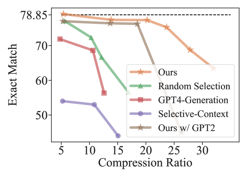
Figure 3: The performance of various prompt compression methods at different compression ratios ($1/\tau$) on GSM8K. The dashed line corresponds to the Exact Match score obtained from the full-shot prompt.

It is shown that as the compression ratio increases especially around 25x-30x, all methods as well as ours will experience a substantial performance drop. In comparison with other methods, this performance drop derived from our approach is significantly shifted to much higher compression ratios. We owe this to the Budget Controller and the Iterative Token-level Prompt Compression algorithm, which enable our method to maintain the original prompt information even at some extreme compression ratios. The upper limit of the compression ratio for different prompts varies, depending on factors such as prompt length, task type, and the number of sentences involved.

Additionally, there may be subtle differences between the tokenizers used by the small language model and the black-box LLM, which may result in an underestimation of the prompt’s token length.

Appendix A Experiment Details

A.1 Dataset Details

GSM8K

A widely used math reasoning dataset comprising 8,000 problems, including a 1,300 problems test set that assesses models’ capabilities in arithmetic reasoning and formulating mathematical steps using language Cobbe et al. (2021). For this dataset, we employ the complex multi-step CoT prompt Fu et al. (2023b) as the original prompt.

BBH

A suite of language and symbolic reasoning tasks, consisting of 6,500 problems across 23 subsets, specifically designed to evaluate chain-of-thought prompting. In our experiment, we adopt the 3-shot CoT prompt as the original prompts, following the approach described by Suzgun et al. (2022).

ShareGPT

A conversation dataset from ShareGPT.com platform sha (2023) which includes users sharing conversations with ChatGPT in different languages and in various scenarios (e.g., coding, chitchat, writing assistant, etc.). We use a dataset of 575 samples provided by Li (2023) as our test set. We use all dialogues except the final round as the prompt and generate results with GPT-3.5-Turbo as the reference.

Arxiv-March23

A dataset consisting of latest academic papers created in March 2023 from the arXiv preprint repository. We use 500 data items collected by Li (2023) as the test set. Due to the excessive length of some articles, we take the first five sections of each article and truncate each section to 10,000 characters. Then, we concatenate these sections to form the original prompt and use GPT-3.5-Turbo to generate the summary as the reference.

A.2 Other Implementation Details

All experiments were conducted using a Tesla V100 (32GB). We trained the GPT2-Alpaca model on the Alpaca dataset for eight epochs using a learning rate of 1e-4 and the AdamW optimizer Loshchilov and Hutter (2019). The training process took approximately 150 minutes to complete. We use tiktoken and GPT-3.5-Turbo model to count all the tokens.

Appendix B Economic Cost

	GSM8K	BBH	ShareGPT	Arxiv
Original	5.2	12.8	0.7	1.3
Ours	0.5	4.8	0.3	0.2

Table 7: The inference costs($) for various datasets using GPT-3.5-Turbo.

Table 7 displays the estimated inference costs for various datasets, according to the pricing of GPT-3.5-Turbo. Our approach showcases significant savings in computational resources and monetary expenditures, with cost reductions of $4.7, $8.0, $0.4, and $0.8 observed in the GSM8K, BBH, ShareGPT, and Arxiv datasets, respectively.

Appendix C Instructions used in GPT-4 Generation

The instructions we used in the GPT-4 Generation are shown below:

1. Could you please rephrase the paragraph to make it short, and keep 5% tokens?

2. Condense the passage to retain only 5% of its original tokens, while preserving its meaning.

3. Short the sentences to 200 tokens.

4. Trim the text down to 200 tokens in total.

5. Please provide a concise summary of the given examples in several sentences, ensuring that all reasoning information is included.

6. Summarize the provided examples in a few sentences, maintaining all essential reasoning aspects.

7. Remove redundancy and express the text concisely in English, ensuring that all key information and reasoning processes are preserved.

8. Eliminate repetitive elements and present the text concisely, ensuring that key details and logical processes are retained.

9. Follow these steps to shorten the given text content: 1. First, calculate the amount of information contained in each sentence, and remove sentences with less information. 2. Next, further condense the text by removing stop words, unnecessary punctuation, and redundant expressions. Refine the content while ensuring that all key information is retained. Let’s do it step by step.

10. To shorten the given text, follow these steps: a) Determine the information value of each sentence and remove those with lower value. b) Further reduce the text by removing stop words, unneeded punctuation, and superfluous expressions, while making sure to keep all vital information intact. Let’s do it step by step.

Appendix D Recovering Compressed Prompts with Large Language Model

In this section, we showcase several examples of employing black-box LLMs to reconstruct compressed prompts. Specifically, we have selected three compressed prompts with varying compression ratios, produced by distinct small language models, on different datasets. These prompts, accompanied by guiding instructions, will serve as input for the GPT-4 model.

Figure 4: Recovering the compressed prompt($1/\tau$=17x, Alpaca-7B as small language model) from GSM8K using GPT-4.

Figure 5: Recovering the compressed prompt ($1/\tau$=19x, GPT2-Alpaca as small language model) from GSM8K using GPT-4.

Figure 6: Recovering the compressed prompt($1/\tau$=7x, Alpaca-7B as small language model) from BBH using GPT-4.

Appendix E Cases Study

We present various cases from multiple datasets, encompassing compressed prompts, outcomes derived from original prompts, outcomes derived from compressed prompts, and results achieved utilizing the selective-context approach.

Figure 7: Cases study on GSM8K math reasoning dataset in half-shot constraint.

Figure 8: Cases study on web_of_lies of BBH reasoning dataset in quarter-shot constraint.

Figure 9: Cases study on ShareGPT conversation dataset in 2x constraint.

Figure 10: Cases study on Arxiv-March23 summarization dataset in 200 tokens constraint.

References

- sha (2023) 2023. Sharegpt. https://sharegpt.com/.
- Arora et al. (2021) Udit Arora, William Huang, and He He. 2021. Types of out-of-distribution texts and how to detect them. In Proceedings of the 2021 Conference on Empirical Methods in Natural Language Processing, pages 10687–10701, Online and Punta Cana, Dominican Republic. Association for Computational Linguistics.
- Bolya et al. (2023) Daniel Bolya, Cheng-Yang Fu, Xiaoliang Dai, Peizhao Zhang, Christoph Feichtenhofer, and Judy Hoffman. 2023. Token merging: Your vit but faster. In The Eleventh International Conference on Learning Representations.
- Chase (2022) Harrison Chase. 2022. LangChain.
- Chevalier et al. (2023) Alexis Chevalier, Alexander Wettig, Anirudh Ajith, and Danqi Chen. 2023. Adapting language models to compress contexts. ArXiv preprint, abs/2305.14788.
- Chiang et al. (2023) Wei-Lin Chiang, Zhuohan Li, Zi Lin, Ying Sheng, Zhanghao Wu, Hao Zhang, Lianmin Zheng, Siyuan Zhuang, Yonghao Zhuang, Joseph E. Gonzalez, Ion Stoica, and Eric P. Xing. 2023. Vicuna: An open-source chatbot impressing gpt-4 with 90%* chatgpt quality.
- Cobbe et al. (2021) Karl Cobbe, Vineet Kosaraju, Mohammad Bavarian, Mark Chen, Heewoo Jun, Lukasz Kaiser, Matthias Plappert, Jerry Tworek, Jacob Hilton, Reiichiro Nakano, et al. 2021. Training verifiers to solve math word problems. ArXiv preprint, abs/2110.14168.
- Delétang et al. (2023) Grégoire Delétang, Anian Ruoss, Paul-Ambroise Duquenne, Elliot Catt, Tim Genewein, Christopher Mattern, Jordi Grau-Moya, Li Kevin Wenliang, Matthew Aitchison, Laurent Orseau, et al. 2023. Language modeling is compression. ArXiv preprint, abs/2309.10668.
- Dettmers et al. (2022) Tim Dettmers, Mike Lewis, Younes Belkada, and Luke Zettlemoyer. 2022. GPT3.int8(): 8-bit matrix multiplication for transformers at scale. In Advances in Neural Information Processing Systems.
- Frantar and Alistarh (2023) Elias Frantar and Dan Alistarh. 2023. SparseGPT: Massive language models can be accurately pruned in one-shot. In International Conference on Machine Learning.
- Frantar et al. (2023) Elias Frantar, Saleh Ashkboos, Torsten Hoefler, and Dan Alistarh. 2023. OPTQ: Accurate quantization for generative pre-trained transformers. In The Eleventh International Conference on Learning Representations.
- Fu et al. (2023a) Yao Fu, Litu Ou, Mingyu Chen, Yuhao Wan, Hao Peng, and Tushar Khot. 2023a. Chain-of-thought hub: A continuous effort to measure large language models’ reasoning performance. ArXiv preprint, abs/2305.17306.
- Fu et al. (2023b) Yao Fu, Hao Peng, Ashish Sabharwal, Peter Clark, and Tushar Khot. 2023b. Complexity-based prompting for multi-step reasoning. In The Eleventh International Conference on Learning Representations.
- Ge et al. (2022) Tao Ge, Jing Hu, Li Dong, Shaoguang Mao, Yan Xia, Xun Wang, Si-Qing Chen, and Furu Wei. 2022. Extensible prompts for language models. ArXiv preprint, abs/2212.00616.
- Ge et al. (2023) Tao Ge, Jing Hu, Xun Wang, Si-Qing Chen, and Furu Wei. 2023. In-context autoencoder for context compression in a large language model. ArXiv preprint, abs/2307.06945.
- Gilbert et al. (2023) Henry Gilbert, Michael Sandborn, Douglas C Schmidt, Jesse Spencer-Smith, and Jules White. 2023. Semantic compression with large language models. ArXiv preprint, abs/2304.12512.
- Goyal et al. (2020) Saurabh Goyal, Anamitra Roy Choudhury, Saurabh Raje, Venkatesan T. Chakaravarthy, Yogish Sabharwal, and Ashish Verma. 2020. Power-bert: Accelerating BERT inference via progressive word-vector elimination. In Proceedings of the 37th International Conference on Machine Learning, ICML 2020, 13-18 July 2020, Virtual Event, volume 119 of Proceedings of Machine Learning Research, pages 3690–3699. PMLR.
- Hu et al. (2022) Edward J Hu, yelong shen, Phillip Wallis, Zeyuan Allen-Zhu, Yuanzhi Li, Shean Wang, Lu Wang, and Weizhu Chen. 2022. LoRA: Low-rank adaptation of large language models. In International Conference on Learning Representations.
- Kim and Cho (2021) Gyuwan Kim and Kyunghyun Cho. 2021. Length-adaptive transformer: Train once with length drop, use anytime with search. In Proceedings of the 59th Annual Meeting of the Association for Computational Linguistics and the 11th International Joint Conference on Natural Language Processing (Volume 1: Long Papers), pages 6501–6511, Online. Association for Computational Linguistics.
- Kim et al. (2022) Sehoon Kim, Sheng Shen, David Thorsley, Amir Gholami, Woosuk Kwon, Joseph Hassoun, and Kurt Keutzer. 2022. Learned token pruning for transformers. In Proceedings of the 28th ACM SIGKDD Conference on Knowledge Discovery and Data Mining, pages 784–794.
- Li (2023) Yucheng Li. 2023. Unlocking context constraints of llms: Enhancing context efficiency of llms with self-information-based content filtering. ArXiv preprint, abs/2304.12102.
- Lin (2004) Chin-Yew Lin. 2004. ROUGE: A package for automatic evaluation of summaries. In Text Summarization Branches Out, pages 74–81, Barcelona, Spain. Association for Computational Linguistics.
- Loshchilov and Hutter (2019) Ilya Loshchilov and Frank Hutter. 2019. Decoupled weight decay regularization. In 7th International Conference on Learning Representations, ICLR 2019, New Orleans, LA, USA, May 6-9, 2019. OpenReview.net.
- Mai et al. (2022) Kimberly T Mai, Toby Davies, and Lewis D Griffin. 2022. Self-supervised losses for one-class textual anomaly detection. ArXiv preprint, abs/2204.05695.
- Modarressi et al. (2022) Ali Modarressi, Hosein Mohebbi, and Mohammad Taher Pilehvar. 2022. AdapLeR: Speeding up inference by adaptive length reduction. In Proceedings of the 60th Annual Meeting of the Association for Computational Linguistics (Volume 1: Long Papers), pages 1–15, Dublin, Ireland. Association for Computational Linguistics.
- Mu et al. (2023) Jesse Mu, Xiang Lisa Li, and Noah Goodman. 2023. Learning to compress prompts with gist tokens. ArXiv preprint, abs/2304.08467.
- Papineni et al. (2002) Kishore Papineni, Salim Roukos, Todd Ward, and Wei-Jing Zhu. 2002. Bleu: a method for automatic evaluation of machine translation. In Proceedings of the 40th Annual Meeting of the Association for Computational Linguistics, pages 311–318, Philadelphia, Pennsylvania, USA. Association for Computational Linguistics.
- Pasco (1976) Richard Clark Pasco. 1976. Source coding algorithms for fast data compression. Ph.D. thesis, Citeseer.
- Rao et al. (2021) Yongming Rao, Wenliang Zhao, Benlin Liu, Jiwen Lu, Jie Zhou, and Cho-Jui Hsieh. 2021. Dynamicvit: Efficient vision transformers with dynamic token sparsification. In Advances in Neural Information Processing Systems.
- Rissanen (1976) Jorma J Rissanen. 1976. Generalized kraft inequality and arithmetic coding. IBM Journal of research and development, 20(3):198–203.
- Shannon (1951) Claude E Shannon. 1951. Prediction and entropy of printed english. Bell system technical journal, 30(1):50–64.
- Sutskever (2023) Ilya Sutskever. 2023. A theory of unsupervised learning. https://simons.berkeley.edu/talks/ilya-sutskever-openai-2023-08-14.
- Suzgun et al. (2022) Mirac Suzgun, Nathan Scales, Nathanael Schärli, Sebastian Gehrmann, Yi Tay, Hyung Won Chung, Aakanksha Chowdhery, Quoc V Le, Ed H Chi, Denny Zhou, , and Jason Wei. 2022. Challenging big-bench tasks and whether chain-of-thought can solve them. ArXiv preprint, abs/2210.09261.
- Taori et al. (2023) Rohan Taori, Ishaan Gulrajani, Tianyi Zhang, Yann Dubois, Xuechen Li, Carlos Guestrin, Percy Liang, and Tatsunori B. Hashimoto. 2023. Stanford alpaca: An instruction-following llama model. https://github.com/tatsu-lab/stanford_alpaca.
- Wei et al. (2022) Jason Wei, Xuezhi Wang, Dale Schuurmans, Maarten Bosma, brian ichter, Fei Xia, Ed H. Chi, Quoc V Le, and Denny Zhou. 2022. Chain of thought prompting elicits reasoning in large language models. In Advances in Neural Information Processing Systems.
- Wingate et al. (2022) David Wingate, Mohammad Shoeybi, and Taylor Sorensen. 2022. Prompt compression and contrastive conditioning for controllability and toxicity reduction in language models. In Findings of the Association for Computational Linguistics: EMNLP 2022, pages 5621–5634, Abu Dhabi, United Arab Emirates. Association for Computational Linguistics.
- Wu et al. (2023) Qianhui Wu, Huqiang Jiang, Haonan Yin, Börje F. Karlsson, and Chin-Yew Lin. 2023. Multi-level knowledge distillation for out-of-distribution detection in text. In Proceedings of the 61th Annual Meeting of the Association for Computational Linguistics (Long Papers).
- Xiao et al. (2023) Guangxuan Xiao, Ji Lin, Mickael Seznec, Julien Demouth, and Song Han. 2023. Smoothquant: Accurate and efficient post-training quantization for large language models. In International Conference on Machine Learning.
- Xu et al. (2023) Can Xu, Qingfeng Sun, Kai Zheng, Xiubo Geng, Pu Zhao, Jiazhan Feng, Chongyang Tao, and Daxin Jiang. 2023. Wizardlm: Empowering large language models to follow complex instructions. ArXiv preprint, abs/2304.12244.
- Yang et al. (2023) Nan Yang, Tao Ge, Liang Wang, Binxing Jiao, Daxin Jiang, Linjun Yang, Rangan Majumder, and Furu Wei. 2023. Inference with reference: Lossless acceleration of large language models. ArXiv preprint, abs/2304.04487.
- Yang et al. (2019) Zhilin Yang, Zihang Dai, Yiming Yang, Jaime G. Carbonell, Ruslan Salakhutdinov, and Quoc V. Le. 2019. Xlnet: Generalized autoregressive pretraining for language understanding. In Advances in Neural Information Processing Systems 32: Annual Conference on Neural Information Processing Systems 2019, NeurIPS 2019, December 8-14, 2019, Vancouver, BC, Canada, pages 5754–5764.
- Zhang et al. (2023) Lei Zhang, Yuge Zhang, Kan Ren, Dongsheng Li, and Yuqing Yang. 2023. Mlcopilot: Unleashing the power of large language models in solving machine learning tasks. ArXiv preprint, abs/2304.14979.
- Zhang et al. (2020) Tianyi Zhang, Varsha Kishore, Felix Wu, Kilian Q. Weinberger, and Yoav Artzi. 2020. Bertscore: Evaluating text generation with BERT. In 8th International Conference on Learning Representations, ICLR 2020, Addis Ababa, Ethiopia, April 26-30, 2020. OpenReview.net.
- Zhou et al. (2023) Wangchunshu Zhou, Yuchen Eleanor Jiang, Ryan Cotterell, and Mrinmaya Sachan. 2023. Efficient prompting via dynamic in-context learning. ArXiv preprint, abs/2305.11170.