Multi-timestep models for Model-based Reinforcement Learning

Abstract

In model-based reinforcement learning (MBRL), most algorithms rely on simulating trajectories from one-step dynamics models learned on data. A critical challenge of this approach is the compounding of one-step prediction errors as length of the trajectory grows. In this paper we tackle this issue by using a multi-timestep objective to train one-step models. Our objective is a weighted sum of a loss function (e.g., negative log-likelihood) at various future horizons. We explore and test a range of weights profiles. We find that exponentially decaying weights lead to models that significantly improve the long-horizon R2 score. This improvement is particularly noticeable when the models were evaluated on noisy data. Finally, using a soft actor-critic (SAC) agent in pure batch reinforcement learning (RL) and iterated batch RL scenarios, we found that our multi-timestep models outperform or match standard one-step models. This was especially evident in a noisy variant of the considered environment, highlighting the potential of our approach in real-world applications.

1 Introduction

Reinforcement learning is a paradigm where a control agent (or policy) learns through interacting with a dynamic system (or environment) and receives feedback in the form of rewards. This approach has proven successful in addressing some of the most challenging problems globally, as evidenced by Silver et al. (2017b; 2018); Mnih et al. (2015); Vinyals et al. (2019). However, reinforcement learning remains largely confined to simulated environments and does not extend to real-world engineering systems. This limitation is primarily due to two factors: i) the scarcity of data resulting from operational constraints, and ii) the safety standards associated with these systems. Model-based reinforcement learning (MBRL) is an approach that can potentially narrow the gap between RL and applications.

Model-based reinforcement learning (MBRL) algorithms alternate two steps: i) model learning, a supervised learning problem to learn the dynamics of the environment, and ii) policy optimization, where a policy and/or a value function is learned by sampling from the learned dynamics. MBRL is recognized for its sample efficiency, as the learning of policy/value is conducted (either wholly or partially) from imaginary model rollouts (also referred to as background planning), which are more cost-effective and readily available than rollouts in the true dynamics (Janner et al., 2019). Moreover, a predictive model that performs well out-of-distribution facilitates easy transfer of the true model to new tasks or areas not included in the model training dataset (Yu et al., 2020).

While model-based reinforcement learning (MBRL) algorithms have achieved significant success, they are prone to compounding errors when planning over extended horizons (Lambert et al., 2022). This issue arises due to the propagation of model bias, leading to highly inaccurate predictions at longer horizons. This can be problematic in real-world applications, as it can result in out-of-distribution states that may violate the physical or safety constraints of the environment. The root of compounding errors is in the nature of the models used in MBRL. Typically, these are one-step models that predict the next state based on the current state and executed action. Long rollouts are then generated by iteratively applying these models, leading to compunding errors. To address this issue, we propose aligning the training objective of these models to optimize the long-horizon error.

Our key contributions are the following:

• We propose a novel training objective for one-step predictive models. It consists in a weighted sum of the loss function at multiple future horizons.

• We perform an ablation study on different strategies to weigh the loss function at multiple future horizons, finding that exponentially decaying weights lead to the best results.

• Finally, we evaluate the multi-timestep models in pure batch and iterated batch MBRL.

2 Related Work

Model-based reinforcement learning

MBRL has been effectively used in iterated batch RL by alternating between model learning and planning (Deisenroth & Rasmussen, 2011; Hafner et al., 2021; Gal et al., 2016; Levine & Koltun, 2013; Chua et al., 2018; Janner et al., 2019; Kégl et al., 2021), and in the offline (pure batch) RL where we do one step of model learning followed by policy learning (Yu et al., 2020; Kidambi et al., 2020; Lee et al., 2021; Argenson & Dulac-Arnold, 2021; Zhan et al., 2021; Yu et al., 2021; Liu et al., 2021; Benechehab et al., 2023). Planning is used either at decision time via model-predictive control (MPC) (Draeger et al., 1995; Chua et al., 2018; Hafner et al., 2019; Pinneri et al., 2020; Kégl et al., 2021), or in the background where a model-free agent is learned on imagined model rollouts (Dyna; Janner et al. (2019); Sutton (1991); Sutton et al. (1992); Ha & Schmidhuber (2018)), or both. For example, model-based policy optimization (MBPO) (Janner et al., 2019) trains an ensemble of feed-forward models and generates imaginary rollouts to train a soft actor-critic agent.

Multi-step predictions

Multi-timestep dynamics modeling was referred to in early works about temporal abstraction (Sutton et al., 1999; Precup et al., 1998) and mixture of timescales models in tabular MDPs (Precup & Sutton, 1997; Singh, 1992; Sutton & Pinette, 1985; Sutton, 1995). It is also partially addressed in the recent MBRL literature by means of recurrent state space models (Hochreiter & Schmidhuber, 1997; Chung et al., 2014; Ha & Schmidhuber, 2018; Hafner et al., 2019; 2021; Silver et al., 2017a). However, these methods rely on heavy computation and approximated inference schemes such as variational inference. The problem of multi-step forecasting was also addressed in the time series literature (Ben Taieb & Bontempi, 2012; Ben Taieb et al., 2012; Venkatraman et al., 2015; Chandra et al., 2021), but none directly aligns the single-step forecasting model training objective to match the multi-step prediction objective, as we propose.

Fixed/variable-horizon architectures

Regarding fixed-horizon models, Asadi et al. (2018; 2019) designed a model that has a distinct neural block for each prediction step, which reduces error accumulation but enlarges the model. Whitney & Fergus (2019) demonstrated that a simple fixed-horizon model has better accuracy and can be used for planning with CEM. However, they had to change the reward function since they did not have access to all the visited states when planning with a fixed-horizon model (discussed in section 4.2). For multi-horizon architectures, Lambert et al. (2021) proposed a model that takes the prediction horizon and the parameters of the current policy as input, instead of the full action sequence. Meanwhile, Whitney & Fergus (2019) used a dynamic-horizon architecture by padding the shorter action sequences with zeros to fit the input size constraint.

Compounding errors in MBRL

Lambert et al. (2022) showed that the stability of the physical system affects the error profile of a model. Talvitie (2014) proposed hallucinated replay, which inputs to the model its own generated (noisy) outputs. This technique teaches the model to recover from its own errors (similar to denoising), and produces models that have lower one-step accuracy but higher returns in some scenarios. A similar idea (multi-step error) is used by Byravan et al. (2021) to train models in the context of MPC, and by Venkatraman et al. (2015) who casts the error-recovery task as imitation learning. In the same vein, Xiao et al. (2023) learned a criterion based on the $h$-step error of the model, and adjusted the planning horizon $h$ accordingly.

3 Preliminaries

The conventional framework used in RL is the finite-horizon Markov decision process (MDP), denoted as $\mathcal{M}=\langle\mathcal{S},\mathcal{A},p,r,\rho_{0},\gamma\rangle$. In this notation, $\mathcal{S}$ is the state space and $\mathcal{A}$ is the action space. The transition dynamics, which could be stochastic, are represented by $p:\mathcal{S}\times\mathcal{A}\leadsto\mathcal{S}$. The reward function is denoted by $r:\mathcal{S}\times\mathcal{A}\rightarrow\mathbb{R}$. The initial state distribution is given by $\rho_{0}$, and the discount factor is represented by $\gamma$, and lies within the range of [0,1].

The objective of RL is to identify a policy $\pi(s)$ which is a distribution over the action space ($\mathcal{A}$) for each state ($s\in\mathcal{S}$). This policy aims at maximizing the expected sum of discounted rewards, denoted as $J(\pi,\mathcal{M}):=\mathbb{E}_{s_{0}\sim\rho_{0},a_{t}\sim\pi,\,s_{t>0}\sim p}[\sum_{t=0}^{H}\gamma^{t}r(s_{t},a_{t})]$, where $H$ represents the horizon of the MDP. Under a given policy $\pi$, the state-action value function (also known as the Q-function) at a specific $(s,a)\in\mathcal{S}\times\mathcal{A}$ pair is defined as the expected sum of discounted rewards. This expectation starts from state $s$, takes action $a$, and follows the policy $\pi$ until termination: $Q^{\pi}(s,a)=\mathbb{E}_{a_{t>0}\sim\pi,s_{t>0}\sim p}\big{[}\sum_{t=0}^{H}\gamma^{t}r(s_{t},a_{t})\mid s_{0}=s,a_{0}=a\big{]}$. Similarly, we can define the state value function by taking the expectation with respect to the initial action $a_{0}$: $V^{\pi}(s)=\mathbb{E}_{a_{t}\sim\pi,s_{t>0}\sim p}\big{[}\sum_{t=0}^{H}\gamma^{t}r(s_{t},a_{t})\mid s_{0}=s\big{]}$.

Model-based RL (MBRL) algorithms address the supervised learning challenge of estimating the dynamics of the environment $\hat{p}$ (and sometimes also the reward function $\hat{r}$) from data collected when interacting with the real system. The loss function is typically the log-likelihood $\mathcal{L}(\mathcal{D};\hat{p})=\frac{1}{N}\sum_{i=1}^{N}\log\hat{p}(s^{i}_{t+1}|s^{i}_{t},a^{i}_{t})$ or Mean Squared Error (MSE) for deterministic models. The learned model can subsequently be employed for policy search under the MDP $\widehat{\mathcal{M}}=\langle\mathcal{S},\mathcal{A},\hat{p},r,\rho_{0},\gamma\rangle$. This MDP shares the state and action spaces $\mathcal{S},\mathcal{A}$, reward function $r$, with the true environment $\mathcal{M}$, but learns the transition probability $\hat{p}$ from the dataset $\mathcal{D}$. The policy $\hat{\pi}=\mathop{\rm argmax}_{\pi}J(\pi,\widehat{\mathcal{M}})$ learned on $\widehat{\mathcal{M}}$ is not guaranteed to be optimal under the true MDP $\mathcal{M}$ due to distribution shift and model bias.

In pure batch (or offline) RL, we are given a set of $N$ transitions $\mathcal{D}=\{(s_{t}^{i},a_{t}^{i},r_{t}^{i},s_{t+1}^{i})\}_{i=1}^{N}$. These transitions are generated by an unknown behavioral policy, $\pi^{\beta}$. The challenge in pure batch RL is to learn a good policy in a single shot, without further interacting with the environment $\mathcal{M}$, even though our objective is to optimize $J(\pi,\mathcal{M})$ with $\pi\not=\pi^{\beta}$.

Similarly to Chua et al. (2018); Kégl et al. (2021), we learn a probabilistic dynamics model with a prediction and an uncertainty on the prediction. Formally, $s_{t+1}\mathrel{\text{\reflectbox{\char 59\relax}}}\hat{p}_{\theta}(s_{t},a_{t})=\mathcal{N}\big{(}\mu_{\theta}(s_{t},a_{t}),\sigma_{\theta}(s_{t},a_{t})\big{)}$, where $\mathcal{N}$ is a multivariate Gaussian, and $\theta$ is the learned parameters of the predictive model. In practical applications, fully connected neural networks are often employed due to their proven capabilities as powerful function approximators (Nagabandi et al., 2018; Chua et al., 2018; Kégl et al., 2021), and their suitability for high-dimensional environments over simpler nonparametric models such as Gaussian processes. Following previous research (Chua et al., 2018; Kégl et al., 2021), we assume a diagonal covariance matrix for which we learn the logarithm of the diagonal entries $\sigma_{\theta}=\mathrm{Diag}(\exp(l_{\theta}))$, where $l_{\theta}$ denotes the output of the neural network.

4 Methods

4.1 Problem statement

In MBRL it is common to use a model $\hat{p}$ that predicts the state one-step ahead $s_{t+1}\mathrel{\text{\reflectbox{\char 59\relax}}}\hat{p}(s_{t},a_{t})$. We train this model to optimize the one-step predictive error $L\big{(}s_{t+1},\hat{p}(s_{t},a_{t})\big{)}$ (MSE or NLL for stochastic modeling) in a supervised learning setting. To learn a policy, we use these models for planning $h$ steps ahead by applying a procedure called rollout: we generate $s_{t+j}\mathrel{\text{\reflectbox{\char 59\relax}}}\hat{p}(s_{t+j-1},a_{t+j-1})$ recursively for $j=1,\ldots,h$. Here $(a_{t},\ldots,a_{t+h-1})={\boldsymbol{a}}_{t:t+h}$ is either a fixed action sequence generated by planning or sampling policy $a_{t+j}\mathrel{\text{\reflectbox{\char 59\relax}}}\pi(s_{t+j})$ for $j=1,\ldots,h$, on the fly. Formally, let

$$\hat{p}^{1}(s_{t},a_{t}) = \hat{p}(s_{t},a_{t})\text{ and }$$ (1)

$$\hat{p}^{j}(s_{t},{\boldsymbol{a}}_{t:t+j}) = \hat{p}\big{(}\hat{p}^{j-1}(s_{t},{\boldsymbol{a}}_{t:t+j-1}),a_{t+j-1}\big{)}\text{ for }j=2,\ldots,h.$$

Using $\hat{p}^{h}(s_{t},{\boldsymbol{a}}_{t:t+h})$ to estimate $s_{t+h}$ is problematic for two reasons:

• A distribution mismatch occurs between the inputs that the model was trained on (sampled from the true unknown transition distribution) and the inputs the model being evaluated on (sampled from the predictive distribution of the model; Talvitie (2014; 2017)).

• The predictive error (and the modeled uncertainty in the case of stochastic models) will propagate through the successive model calls, leading to compounding errors (Lambert et al., 2022; Talvitie, 2014; Venkatraman et al., 2015).

To mitigate these issues, we propose models that learn to predict the state $s_{t+h}$ after an arbitrary future horizon $h$ given $s_{t}$ and an action sequence ${\boldsymbol{a}}_{t:t+h}$. We identify two levels in addressing the stated problem:

1. First we build direct models $\hat{p}_{h}(s_{t},{\boldsymbol{a}}_{t:t+h})$ that predict the state at a fixed future horizon $h$ (similar to Whitney & Fergus (2019)). These models cannot directly be used for planning since they do not give access to intermediate rewards $(r_{t+1},\ldots,r_{t+h-1})$, but they serve to motivate the second level, our main contribution:

2. We build one-step models $\hat{p}$ but train them to predict the $h$-step error (2) using the recursive formula (1). Since $\hat{p}$ is a neural net, here we are essentially using recurrent nets.

We start our analysis from Level 1 in Section 4.2, and address Level 2 in Section 4.3. Finally, the experimental setup and the performance evaluation of the agents and our proposed models is showcased in Section 5.

4.2 Fixed-horizon models

Fixed-horizon models $\hat{p}_{h}$ take as input the current state $s_{t}$ and an action sequence ${\boldsymbol{a}}_{t:t+h}=(a_{t},\ldots,a_{t+h-1})$, and predict the parameters of a diagonal multi-variate Gaussian distribution over the state observed $h$ steps into the future: $\hat{s}_{t+h}\sim\mathcal{N}(\hat{\mu}_{\theta}(s_{t},{\boldsymbol{a}}_{t:t+h}),\hat{\sigma}_{\theta}(s_{t},{\boldsymbol{a}}_{t:t+h}))$ with $\theta$ representing the parameters of $\hat{p}_{h}$.

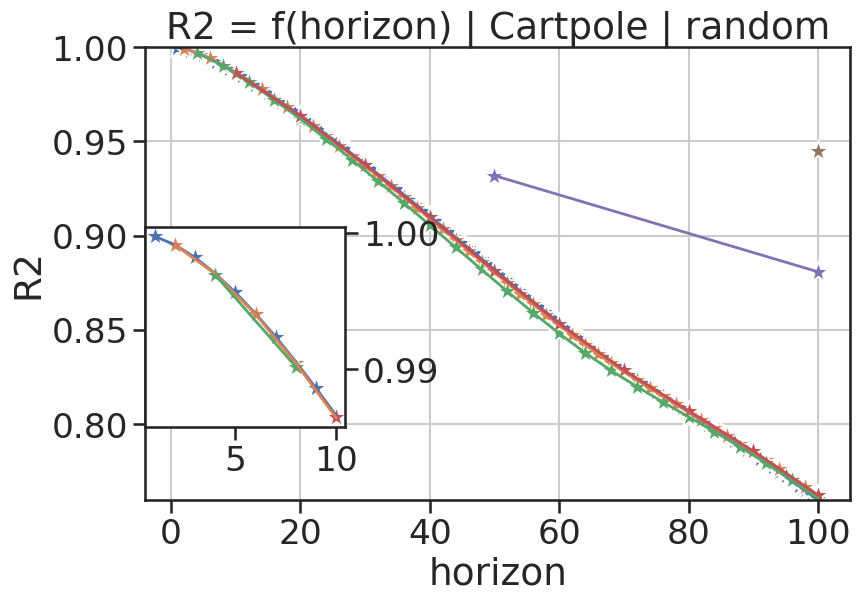
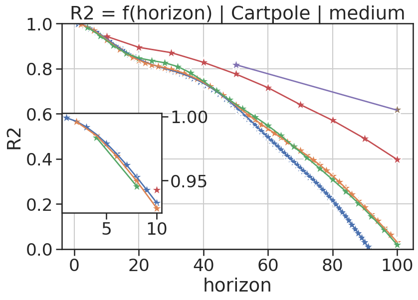
Figure 1: R2 score (explained variance) as a function of the prediction horizon for several multi-step models. We use prediction horizons $h\in\{1,2,4,10,50,100\}$, and apply the predictors recursively according to (1) up to maximum horizon $H=100$. The difference between the two plots is the evaluation dataset: random (where the behaviour policy is a random policy) and medium (where the behaviour policy is a half-expert policy). A discussion on the differences between these datasets is given in Appendix A.2.

Figure 1 shows the error at different horizons for different fixed-horizon models and datasets. For each horizon $h$, the error is computed by considering all sub-trajectories of size $h$ from the test set. We call each $h$-step model $\hat{p}_{h}$ recursively $H/h$ times to compute the prediction $\hat{p}_{h}^{H/h}$ up to $H$ steps ahead.

In general, for a given horizon, we observe that the R2 score (explained variance) increases as we go from the one-step model to the hundred-step model. For the Cartpole random dataset, the short-horizon models are almost identical, while the fifty- and the hundred-step models achieve distinguishable R2 scores. In the medium dataset the improvement grows steadily with $h$.

4.3 Training the one-step models with the error $h$ steps ahead

Figure 1 shows that it may be worthy to train models for longer horizons. But, since our goal is to plan with an arbitrary horizon, we wanted to improve the one-step predictor $\hat{p}$ rather than throwing it away. An obvious solution was to train the recurrent predictor $\hat{p}^{h}$ to minimize $L\big{(}s_{t+h},\hat{p}^{h}(s_{t},{\boldsymbol{a}}_{t:t+h})\big{)}$, but we found that this made the one-step prediction worse, even for the minimal case of $h=2$ (Figure 2 with $\alpha=0$). As can be seen from the same figure, in both medium and random datasets the models where $\alpha<1.0$, suffer a worse predictive error for short horizons, but recover and beat the vanilla one-step model down-the-horizon.

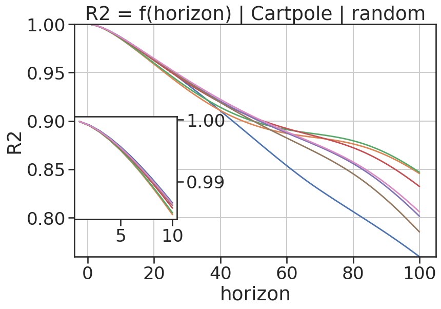
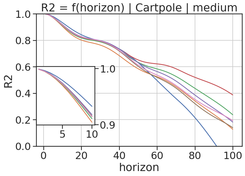
Figure 2: R2 score (explained variance) as a function of the prediction horizon for different weight vectors of ${\boldsymbol{\alpha}}=[\alpha,1-\alpha]$. $\hat{p}$ is learned minimizing $\alpha\times L\big{(}s_{t+1},\hat{p}(s_{t},a_{t})\big{)}+(1-\alpha)\times L\Big{(}s_{t+2},\hat{p}\big{(}\hat{p}(s_{t},a_{t}),a_{t+1}\big{)}\Big{)}$.

Following the empirical findings in the previous simple case, we hypothesize that the solution is to force the predictor $\hat{p}$ to be good on all horizons. Formally, we define horizon-dependent weights ${\boldsymbol{\alpha}}=(\alpha_{1},\ldots,\alpha_{h})$, and minimize the loss

$$L_{\boldsymbol{\alpha}}\big{(}{\boldsymbol{s}}_{t+1:t+h+1},\hat{p}^{1:h}(s_{t},{\boldsymbol{a}}_{\cdot})\big{)}=\sum_{j=1}^{h}\alpha_{j}L\big{(}s_{t+j},\hat{p}^{j}(s_{t},{\boldsymbol{a}}_{t:t+j})\big{)}.$$ (2)

To proceed with gradient descent-based optimization, we only need the gradient of the loss with respect to the model’s parameters. Therefore, we provide an analysis of the analytical gradient of this loss in Appendix C. We derive the gradient in equation 6 to highlight the fact that unlike existing literature (hallucinated replay Talvitie (2014) and multi-step loss Byravan et al. (2021)), our proposed method consists in back-propagating the gradient of the loss through the successive compositions of the model ($\hat{p}^{1:h}(s_{t},{\boldsymbol{a}}_{\cdot})$) figuring in $L_{\boldsymbol{\alpha}}$. Furthermore, we find that the derivative of the generalized loss $L_{\boldsymbol{\alpha}}$ can be expressed as a linear function of the derivative of the loss one-step ahead $L\big{(}s_{t+1},\hat{p}(s_{t},a_{t})\big{)}$. This opens the door for gradient approximation ideas that are briefly discussed in Appendix C, and intended to be explored in future follow-up works.

An important matter that remains to solve is the choice of the weights $\{\alpha_{j}\}_{j\in\{1,\ldots,h\}}$. For instance, Figure 2 shows that for $h=2$ the best weight vector ${\boldsymbol{\alpha}}=(\alpha,1-\alpha)$ depends on both the horizon and the dataset, and that it is neither $[1,0]$ (the classical $\hat{p}$ trained for one-step error), nor $[0,1]$ ($\hat{p}$ trained to minimize $L\Big{(}s_{t+2},\hat{p}\big{(}\hat{p}(s_{t},a_{t}),a_{t+1}\big{)}\Big{)}$). In the next section, we present multiple choices for the weights $\alpha_{j}$, along with the intuition behind each one of them.

4.3.1 How to choose $\{\alpha_{j}\}_{j\in\{1,\ldots,h\}}$ ?

The choice of $\alpha_{j}$ is very important in this context as it allows us to balance the optimization problem between losses at different prediction horizons. In fact, the different loss terms are at different scales since the error grows with the prediction horizon, and therefore a sensible choice of these weights is critical.

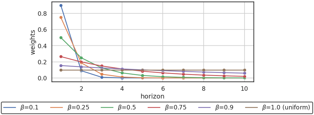
Figure 3: For a maximum horizon of $10$, the figure shows the different weight profiles that we get by varying the decay parameter $\beta$.

• Uniform. $\alpha_{j}=1/h$ The most intuitive way to handle the weighting of the losses is by using uniform weights. However, this method can be sub-optimal since the loss terms $L\big{(}s_{t+j},\hat{p}^{j}(s_{t},{\boldsymbol{a}}_{t:t+j})\big{)}$ grow with $j$ so in a flat sum long horizon errors will dominate.

• Decay. $\alpha_{j}=(\frac{1-\beta}{1-\beta^{h+1}})\beta^{j}$ This method implements an exponential decay through a parameter $\beta$ (Figure 3 shows the weight profiles obtained using different values of $\beta$).

• Learn. $\alpha_{j}=learnable$ In this setting, the $\alpha_{j}$ are left as free-parameters to be learned by the model. The expected outcome in this case is that the model puts the biggest weight on the one-step error $L\big{(}s_{t+1},\hat{p}(s_{t},a_{t})\big{)}$ as it’s smaller than further horizons.

• Proportional. $\alpha_{j}\sim\frac{1}{L\big{(}s_{t+j},\hat{p}^{j}(s_{t},{\boldsymbol{a}}_{t:t+j})\big{)}}$ This method normalizes all the loss terms with their amplitude so that they become equivalent optimization-wise.

5 Experiments & Results

This section starts by presenting the experimental setup, followed by the experiments we conducted to evaluate the proposed models.

5.1 Experimental setup

We are interested in testing our models in two ways: “static” model learning from a fixed data set, and “dynamic” agent learning from model-generated traces. While we are interested in building models that improve the predictive error beyond the one-step transition, the relationship between this surrogate metric and the return of the underlying agent is not trivial. Indeed, in many scenarios, models that have lower predictive ability lead to better performing agents (Talvitie, 2014).

Therefore, we suggest the following experimental settings:

• Pure batch (offline) RL. In this setting, we dispose of multiple datasets with different characteristics. We then test the predictive error of our models against these datasets in a supervised-learning fashion. The main metric in this setting is the R2 score that we evaluate at different future horizons. The resulting models can then be used to train an RL agent (We use Soft-Actor Critic, implementation details can be found in Appendix B) in what can be seen as a single-iteration MBRL.

• Iterated batch RL. In this setting, we alternate between generating a system trace (one episode from the real system), training the model using the traces collected so-far, and training the policy (RL agent) on the freshly updated model. We measure dynamic metrics such as the convergence pace and the mean asymptotic reward or return.

We conduct our experiments in the continuous control environment Cartpole swing-up. We use the implementation of Deepmind Control (Tassa et al., 2018) which is based on the Mujoco physics simulator (Todorov et al., 2012). A description of this environment can be found in Appendix A. A detailed comparison of the static datasets used in the pure batch RL setting is given in Appendix A.2.

Noisy Environment

In an effort to further examine the applicability of multi-timestep models, we suggest the use of a Cartpole swing-up variant that is characterized by the addition of Gaussian noise with a fixed standard deviation (equal to $1\%$ of the range of a given variable) to all observable variables. The Noisy Cartpole environment is of particular interest due to the potential for multi-timestep models to experience significant failures as a result of the accumulation of substantial noise on the learning targets projected $h$ steps ahead. We aim at demonstrating that our proposed method effectively addresses this problem by introducing self-consistency through the concurrent optimization of errors for future horizons.

5.2 Static evaluation: R2 on fixed datasets

For each horizon $j$, the error is computed by considering all the sub-trajectories of size $j$ from the Test dataset. The predictions are then computed by $j$ model compositions (using the groundtruth actions) and the average R2 score is reported.

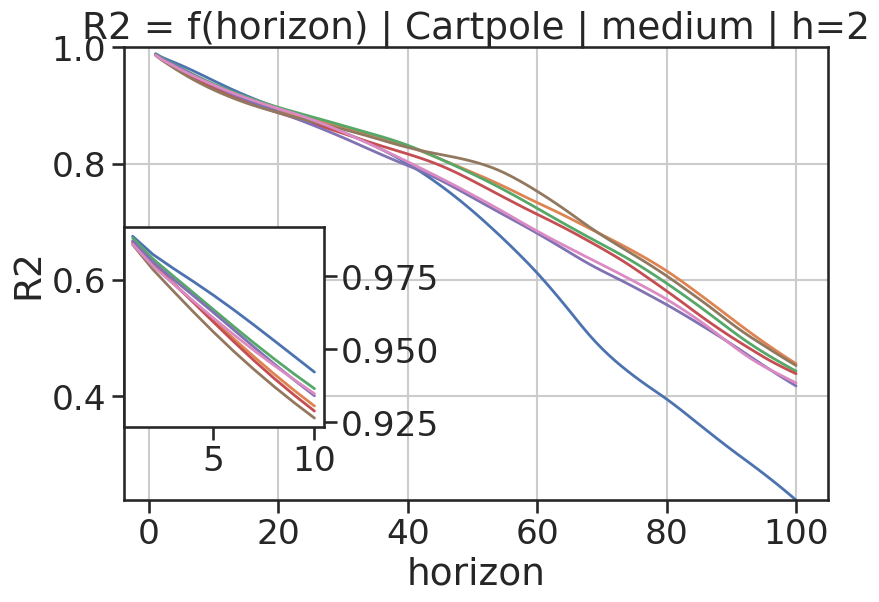
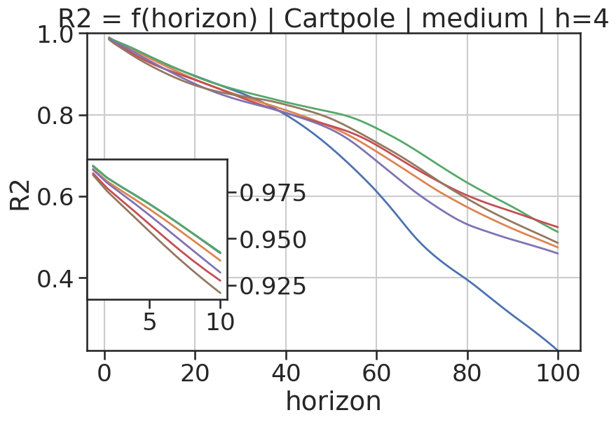
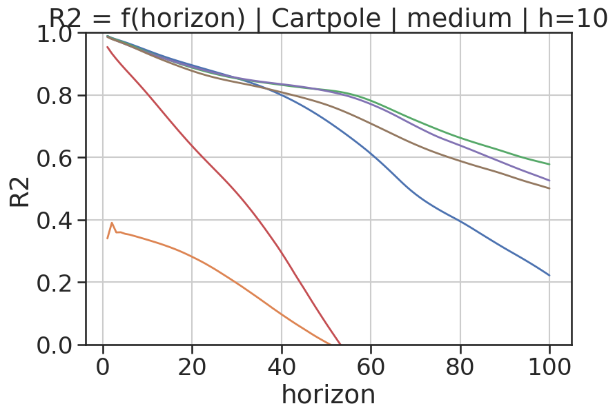
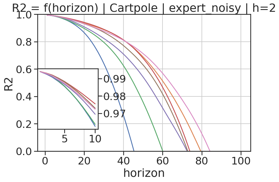
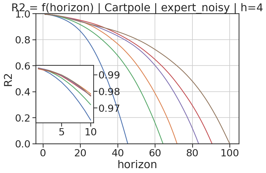
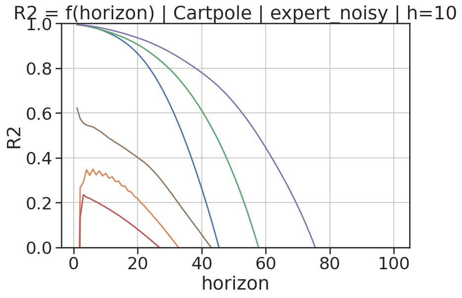
Figure 4: For different maximum horizons $h\in\{2,4,10\}$ represented by columns, and datasets (medium and expert_noisy) represented by rows, we show the R2 score as a function of the prediction horizon for different weight profiles.

Figure 4 shows the R2 score as a function of the prediction horizon, when using multiple weight profiles for three maximum horizons models: $h\in\{2,4,10\}$. In both the medium and expert_noisy datasets, the multi-timestep models largely improve over the vanilla one-step model. Depending on the future horizons scope, we obtain different optimal weight profiles (mostly from the noisy dataset as in the noiseless one the differences are minor): $decay(\beta=0.9)$ for $h=2$, $decay(\beta=0.75)$ for $h=4$, and $decay(\beta=0.3)$ for $h=10$. We interpret the effectiveness of the $decay$ weighting schema from the error profile witnessed for the one-step model. Indeed, the error for this model grows exponentially with the prediction horizon (a theoretical justification can be found in Theorem 1 of Venkatraman et al. (2015)), suggesting that exponentially decaying weights (modulo the right parameter $\beta$) can correctly balance the training objective.

Inspired by this finding, we investigated the direct use of weights that are the exact inverse of the loss term they correspond to ($\alpha_{j}=proportional$). However, this technique didn’t further improve the results. A potential explanation is the interdependence between the different losses as reducing one loss can indirectly affect another one.

Unsurprisingly, the learnable weighting profile quickly converges to putting most of the weight on the one-step error, this is expected because the one-step loss is the smallest among the other terms. A potential fix to this phenomena is to add a regularization term that enforces the weights to be more equally distributed. The elaboration of this idea is beyond the scope of this work.

5.3 Dynamic evaluation: pure batch (offline) RL

To demonstrate the effectiveness of multi-timestep models in practical RL scenarios, we start with the pure batch RL setting. Using the medium, random, and expert datasets for the Cartpole swing-up environment, and the expert_noisy dataset for its noisy variant. We train SAC agents on models that are themselves trained on these respective datasets, and evaluate them on the real system. Regarding the multi-timestep models, we choose the best model on each maximum horizon ($decay(\beta=0.9)$ for $h=2$, $decay(\beta=0.75)$ for $h=4$, and $decay(\beta=0.3)$ for $h=10$), and the vanilla one-step model for comparison.

Table 1: Pure batch (offline) RL evaluation: mean $\pm$ $90\%$ Gaussian confidence interval over 3 seeds. The reported score is the episodic return after training SAC on the pre-trained models for $500k$ steps

Model	medium	expert_noisy	random	expert
$h=1$	813.4 $\pm$ 19.8	580.3 $\pm$ 56.7	308.7 $\pm$ 20.4	807.3 $\pm$ 57.1
$h=2|\alpha=decay(\beta=0.9)$	812.8 $\pm$ 32.2	538.8 $\pm$ 75.8	214.5 $\pm$ 71.1	830.6 $\pm$ 44.2
$h=4|\alpha=decay(\beta=0.75)$	832.0 $\pm$ 35.7	639.09 $\pm$ 22.5	178.9 $\pm$ 29.2	822.1 $\pm$ 56.6
$h=10|\alpha=decay(\beta=0.3)$	842.4 $\pm$ 36.2	557.7 $\pm$ 141.2	208.3 $\pm$ 42.4	730.2 $\pm$ 147.8

Although the results are not yet statistically significant due to a limited number of seeds, multi-timestep models improve over the one-step model in the datasets that require long-horizon accuracy (all but the random dataset where the policy keeps navigating the same region around the initial states).

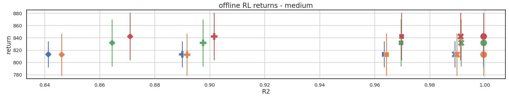
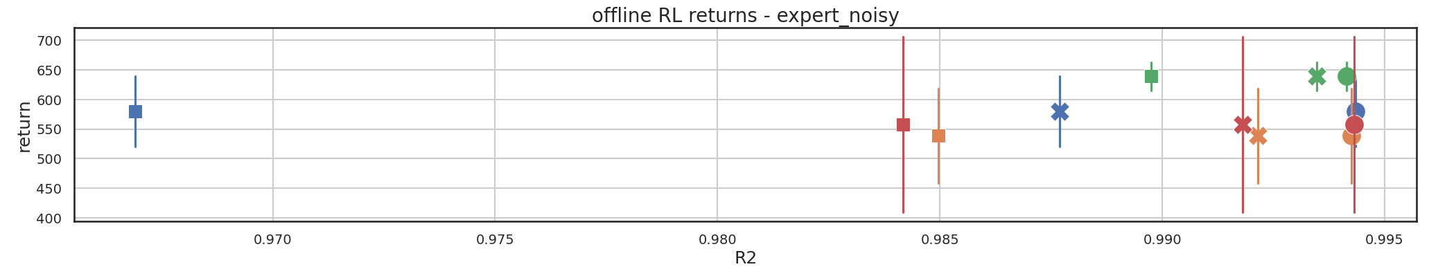
Figure 5: The average episodic return as a function of the R2 score at different horizons $h\in\{1,5,10,25,50\}$. We show this for both the medium dataset representing the vanilla Cartpole environment, and expert_noisy for its noisy variant. We omit the longer horizons ($25$ and $50$) in the second plot as the corresponding R2 scores become out of scale.

To get insights about the relationship between the average episodic returns of the final agents, and the predictive error of the underlying models, we propose the experiment in Figure 5. For all prediction horizons $h\in\{1,5,10,25,50\}$, we can see that in the medium dataset, the $R2(h)$ scores of the different models are positively correlated with their corresponding return. However, in the noisy dataset the relationship is not obvious. The interpretation of this empirical finding is not trivial as many factors are involved. However, a potential explanation is that related to the noise level of the environments. Indeed, models trained on noisy datasets may overfit the noise leading to worse generalizability, and consequently, worse agents in terms of the episodic return.

5.4 Dynamic evaluation: Iterated batch RL

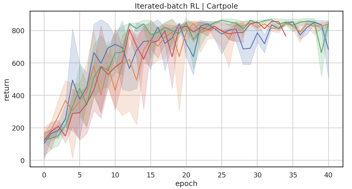
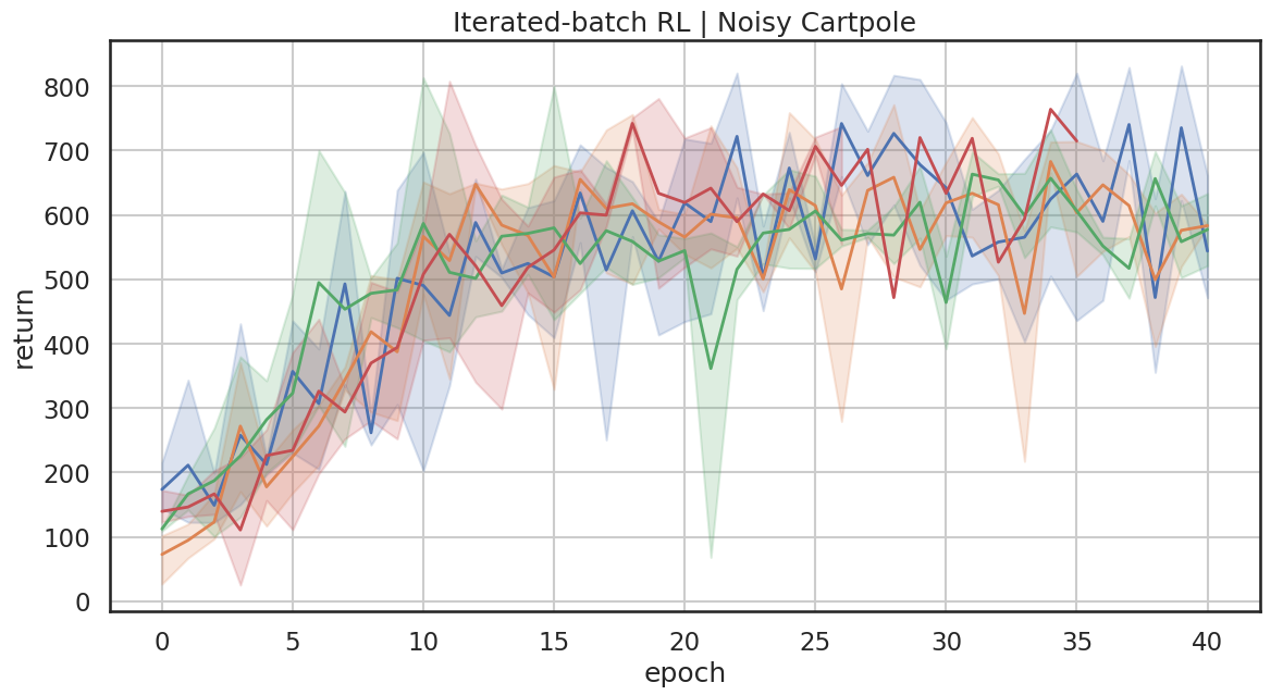
Figure 6: The iterated-batch RL results for the different multi-timestep models in comparison with the standard one-step model. We report the mean $\pm$ standard deviation across 3 seeds. The epoch in the x-axis denotes one iteration of the MBRL loop: model training on the dataset collected so far + Agent learning on model rollouts + evaluating the agent in the real system and updating the dataset.

Finally, we run the full iterated batch MBRL (iterating between model learning, agent learning, and data collection) with the best multi-timestep models and compare the results with the vanilla one-step models in Figure 6. In this setting, the improvement brought by the multi-timestep models is not significant as the episodic return show a large variance among all the models.

6 Conclusion

In this paper, we ask how to adjust the training objective of one-step predictive models to be good at generating long rollouts during planning in model-based reinforcement learning. We build on the observation that fixed-horizon models achieve a lower predictive error down-the-horizon, and adapt the idea in the form of a novel training objective for one-step models. Our idea, which materialises in a weighted sum of the loss functions at future prediction horizons, led to models that, when evaluated against noiseless and noisy datasets from the Cartpole benchmark, show a large improvement of the R2 score compared to the vanilla one-step model. This improvement translates into better agents in pure batch (offline) RL. While the method did not improve the performance in the iterated batch setup, it did not lower the performance either. We will analyze in future work what confounding factors did not make performances improve.

One of the main research directions that follow-up from this work is the exploitation of gradient approximation schemes in the case of deterministic models. Indeed, as demonstrated in appendix C, the analytical form of our proposed loss function simplifies nicely as a linear function of the standard one-step loss. Furthermore, we plan to continue evaluating the resulting multi-timestep models in different settings/environments, and test their integration with state-of-the-art MBRL algorithms that rely on single-step dynamics models.

Limitations

There are two major limitations of this study that could be addressed in future research. First, the study focused solely on the Cartpole benchmark, a relatively low-dimensional environment that reduces the modelling complexity that may be encountered in other high-dimensional systems. Nevertheless, to improve the generalisability of our results, we used different offline datasets and considered a more challenging Cartpole variant with additive Gaussian noise. Second, since our proposed objective can be plugged into any single-step model-based algorithm, we believe it would be interesting to test its integration with some of the state-of-the-art MBRL algorithms in different setups/applications. This is particularly important as our experiments in the offline and iterated-batch settings did not show a statistically significant improvement. Nevertheless, in this work we showcased the importance of multi-timestep models for the dynamics modeling task using different challenging setups, suggesting that they may well find RL applications, where the dynamics modeling is crucial for the final task.

Reproducibility Statement

In order to ensure reproducibility we will release the code at <URL hidden for review>, once the paper has been accepted. The implementation details and hyperparameters are listed in Appendix B.

Appendix A The Cartpole Reinforcement Learning Benchmark

A.1 The environment

Figure 7: The cartpole environment.

The Cartpole swing-up environment is characterized by a five-dimensional state space and a single-dimensional action space. The action in this environment consists of applying a horizontal force to the base of the cart, with the force ranging from -1 to 1. The task horizon is set to 1000. The reward function is designed to encourage the system to remain upright and centered, with small action and velocity values. The observables for this environment include the x-coordinate, the cosine and sine of the pole angle, the x velocity, and the pole’s angular velocity. These parameters collectively define the dynamics and objectives of the Cartpole swing-up task.

A.2 The Offline cartpole datasets

In this section, we introduce the different datasets that are used to evaluate the multi-timestep models on the Cartpole (swingup) environment. These datasets are collected using some behaviour policies that are considered unknown to the agent (the combination of the world model and the actor that is using it for planning). All the datasets consist of $50$ episodes ($50k$ steps) split randomly as following: $36$ episodes for training, $4$ episodes for validation, and the remaining $10$ episodes are used for testing.

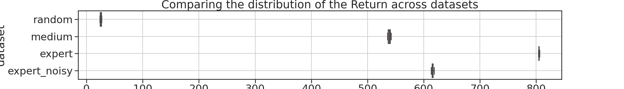
Figure 8: A comparison of the distribution of returns across the considered datasets.

We dispose of four datasets:

• random. This dataset is collected using a random policy (a policy that samples actions uniformly from the action space).

• medium. This is an intermediate between the two. It is collected by an unstable SAC agent that sometimes reaches near-optimal behaviour and sometimes doesn’t manage to.

• expert. This is the full learning trace of an expert-policy (a Soft Actor-Critic -SAC- that is trained on an autoregressive mixture density network until convergence).

• expert_noisy. This is the full learning trace of the expert policy in the noisy Cartpole environment.

To understand the differences between these datasets we propose to analyze the variance of each state dimension of the Cartpole observables. We can see from Figure 9 that the expert dataset has very little variance as it converges quickly (around episode $8$) and all the remaining episodes are almost identical. Similarly, the random dataset has little variance as it keeps exploring the same region around the initial state. The medium dataset, and naturally the expert_noisy dataset are the most diverse among the four, and we believe it would be insightful to evaluate the multi-timestep models against these different challenges, both in terms of the predictive error, and the final return of the underlying agents.

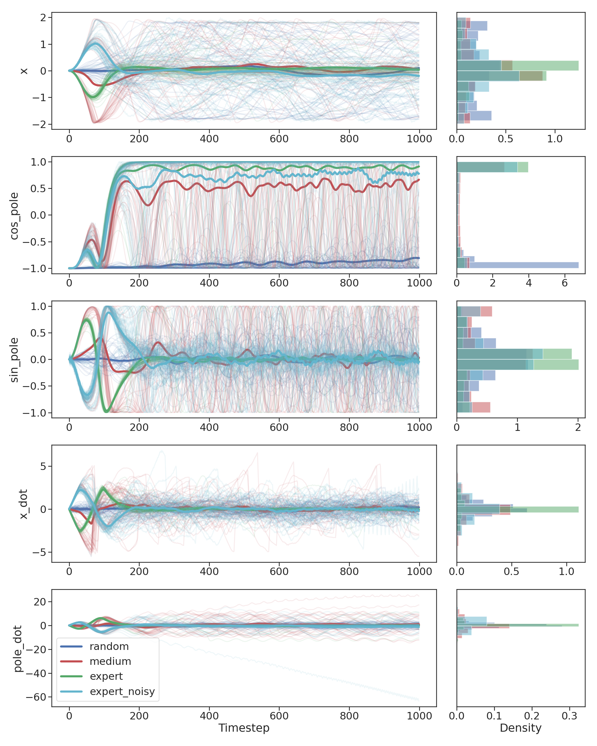
Figure 9: A comparison of the distribution of the state observables across the considered datasets.

Appendix B Implementation details

For all the models, we use a neural network composed of a common number of hidden layers and two output heads (with Tanh activation functions) for the mean and standard deviation of the learned probabilistic dynamics (The standard deviation is fixed when we want to use the MSE loss). We use batch normalization (Ioffe & Szegedy, 2015), Dropout layers (Srivastava et al., 2014) ($p=10\%$), and set the learning rate of the Adam optimizer (Kingma & Ba, 2015) to $0.001$, the batch size to $64$, the number of common layers to $2$, and the number of hidden units to $256$ based on a hyperparameter search executed using the RAMP framework (Kégl et al., 2018). The evaluation metric of the hyperparameter optimization is the aggregated validation R2 score across all the offline datasets.

For the offline and iterated-batch RL experiments, we use SAC agents from the open-source library StableBaselines3 (Raffin et al., 2021) while keeping its default hyperparameters. In the offline setting, we train the SAC agents for $500k$ steps on a fixed model, and evaluate them by rolling-out an episode in the real environment. In the iterated-batch setting, the episodes generated from the evaluation of SAC are added to the current data buffer and used to retrain the model from scratch. For both these setups, we modify the dynamics models to predict the state difference rather than the raw next state: $s_{t+1}\mathrel{\text{\reflectbox{\char 59\relax}}}\hat{p}(s_{t},a_{t})+s_{t}$. This simple technique has been proved to improve the results of MBRL algorithms (Chua et al., 2018).

Appendix C Gradient computation

In this section we want to compute the analytic derivative of the generalized loss: $L_{\boldsymbol{\alpha}}\big{(}{\boldsymbol{s}}_{t+1:t+h+1},\hat{p}^{1:h}(s_{t},{\boldsymbol{a}}_{\cdot})\big{)}=\sum_{j=1}^{h}\alpha_{j}L\big{(}s_{t+j},\hat{p}^{j}(s_{t},{\boldsymbol{a}}_{t:t+j})\big{)}$ with respect to a model parameter $\theta$. For simplicity we denote the j-step loss $L^{(j)}=L\big{(}s_{t+j},\hat{p}^{j}(s_{t},{\boldsymbol{a}}_{t:t+j})\big{)}$ and omit actions from the j-step prediction function: $\hat{p}^{j}(s_{t})$. Under the assumption of a single-dimensional state and MSE loss, we derive the formula of $\frac{d}{d\theta}L^{(j)}$ for $j\in\{1,\ldots,h\}$:

$$\begin{split}\frac{d}{d\theta}[L^{(j)}]&=\frac{d}{d\theta}[(\hat{p}_{\theta}^{j}(s_{t})-s_{t+j})^{2}]\\ &=2\frac{d}{d\theta}[\hat{p}_{\theta}^{j}(s_{t})](\hat{p}_{\theta}^{j}(s_{t})-s_{t+j})\\ &=2\frac{d}{d\theta}[\hat{p}_{\theta}(\hat{p}_{\theta}^{j-1}(s_{t}))](\hat{p}_{\theta}^{j}(s_{t})-s_{t+j})\\ &=2\frac{d}{d\theta}[\hat{p}_{\theta}^{j-1}(s_{t})]\frac{d}{d\theta}[\hat{p}_{\theta}]\big{(}\hat{p}_{\theta}^{j-1}(s_{t})\big{)}(\hat{p}_{\theta}^{j}(s_{t})-s_{t+j})\\ &=2\left(\prod_{i=0}^{j-1}\frac{d}{d\theta}[\hat{p}_{\theta}]\big{(}\hat{p}_{\theta}^{i}(s_{t})\big{)}\right)(\hat{p}_{\theta}^{j}(s_{t})-s_{t+j})\hskip 11.38092pt\text{(by recursion)}\end{split}$$ (3)

From this we can compute the gradient of the loss $\frac{d}{d\theta}L_{\boldsymbol{\alpha}}$:

$$\begin{split}\frac{d}{d\theta}\mathcal{L}&=\sum_{j=1}^{n}\alpha_{j}\frac{d}{d\theta}L^{(j)}\\ &=2\sum_{j=1}^{n}\alpha_{j}\left(\prod_{i=0}^{j-1}\frac{d}{d\theta}[\hat{p}_{\theta}]\big{(}\hat{p}_{\theta}^{i}(s_{t})\big{)}\right)(\hat{p}_{\theta}^{j}(s_{t})-s_{t+j})\end{split}$$ (4)

We start by observing that the terms featuring in the product are cumulative as we go further in the horizon. We thus compute the ratio between two consecutive loss terms $L^{(j-1)}$ and $\mathcal{L}^{(j)}$:

$$\begin{split}\frac{\frac{d}{d\theta}L^{(j)}}{\frac{d}{d\theta}L^{(j-1)}}&=\frac{2\left(\prod_{i=0}^{j-1}\frac{d}{d\theta}[\hat{p}_{\theta}]\big{(}\hat{p}_{\theta}^{i}(s_{t})\big{)}\right)(\hat{p}_{\theta}^{j}(s_{t})-s_{t+j})}{2\left(\prod_{i=0}^{j-2}\frac{d}{d\theta}[\hat{p}_{\theta}]\big{(}\hat{p}_{\theta}^{i}(s_{t})\big{)}\right)(\hat{p}_{\theta}^{j-1}(s_{t})-s_{t+j-1})}\\ &=\frac{d}{d\theta}[\hat{p}_{\theta}]\big{(}\hat{p}_{\theta}^{j-1}(s_{t})\big{)}\frac{(\hat{p}_{\theta}^{j}(s_{t})-s_{t+j})}{(\hat{p}_{\theta}^{j-1}(s_{t})-s_{t+j-1})}\end{split}$$ (5)

Given equation 5, we can write a formula for $\frac{d}{d\theta}L_{\boldsymbol{\alpha}}$ that only depends on the prediction one-step ahead and its gradient. We denote the error ratio between horizons $k$ and $l$: $Err_{(k,l)}=\frac{(\hat{p}_{\theta}^{l}(s_{t})-s_{t+l})}{(\hat{p}_{\theta}^{k}(s_{t})-s_{t+k})}$; And the gradient of the prediction function evaluated at the $k$-th horizon: $G_{k}=\frac{d}{d\theta}[\hat{p}_{\theta}]\big{(}\hat{p}_{\theta}^{k}(s_{t})\big{)}$. We use the convention that $G_{0}=1$ and $Err_{(0,1)}=1$.

Let’s refactor the expression of the gradient $\frac{d}{d\theta}L_{\boldsymbol{\alpha}}$ in equation 4 using the ratio from equation 5:

$$\begin{split}\frac{d}{d\theta}L_{\boldsymbol{\alpha}}&=\sum_{j=1}^{n}\alpha_{j}\frac{d}{d\theta}L^{(j)}\\ &=\alpha_{1}\frac{d}{d\theta}L^{(1)}+\sum_{j=2}^{h}\alpha_{j}\frac{d}{d\theta}[\hat{p}_{\theta}]\big{(}\hat{p}_{\theta}^{j-1}(s_{t})\big{)}\frac{(\hat{p}_{\theta}^{j}(s_{t})-s_{t+j})}{(\hat{p}_{\theta}^{j-1}(s_{t})-s_{t+j-1})}L^{(j-1)}\\ &=\alpha_{1}\frac{d}{d\theta}L^{(1)}+\sum_{j=2}^{h}\alpha_{j}G_{j-1}Err_{(j-1,j)}L^{(j-1)}\\ &=\alpha_{1}\frac{d}{d\theta}L^{(1)}+\sum_{j=1}^{h-1}\alpha_{j+1}G_{j}Err_{(j,j+1)}L^{(j)}\\ &=\alpha_{1}\frac{d}{d\theta}L^{(1)}+\alpha^{2}G_{1}Err_{(1,2)}\frac{d}{d\theta}L^{(1)}+\sum_{j=2}^{n}\alpha_{j}G_{j-1}Err_{(j-1,j)}L^{(j-1)}\\ &=\sum_{j=1}^{h}\alpha_{j}\left(\prod_{i=0}^{j-1}G_{i}\right)\left(\prod_{i=0}^{j-1}Err_{(i,i+1)}\right)\frac{d}{d\theta}L^{(1)}\hskip 14.22636pt\text{(by recursion)}\\ &=\sum_{j=1}^{h}\alpha_{j}\left(\prod_{i=0}^{j-1}G_{i}\right)\left(Err_{(1,h)}\right)\frac{d}{d\theta}L^{(1)}\hskip 14.22636pt\text{(Elements simplify by definition of $Err_{(i,i+1)}$)}\end{split}$$ (6)

This formulation expresses the generalized loss derivative as a linear function of the derivative of the loss one-step ahead. The latter is relatively cheap and can be computed with one forward (and backward) pass through the model. Consequently, we can think of approximation schemes to reduce the computational burden $O(n\times Cost(L^{(1)}))$ that comes with computing the full derivative: $\frac{d}{d\theta}L_{\boldsymbol{\alpha}}$. We leave the exploration of this idea to a future follow-up work.

References

- Argenson & Dulac-Arnold (2021) Arthur Argenson and Gabriel Dulac-Arnold. Model-based offline planning. In International Conference on Learning Representations, 2021.
- Asadi et al. (2018) Kavosh Asadi, Evan Cater, Dipendra Misra, and Michael L. Littman. Towards a Simple Approach to Multi-step Model-based Reinforcement Learning, October 2018. URL http://arxiv.org/abs/1811.00128. arXiv:1811.00128 [cs, stat].
- Asadi et al. (2019) Kavosh Asadi, Dipendra Misra, Seungchan Kim, and Michel L. Littman. Combating the Compounding-Error Problem with a Multi-step Model, May 2019. URL http://arxiv.org/abs/1905.13320. arXiv:1905.13320 [cs, stat].
- Ben Taieb & Bontempi (2012) Souhaib Ben Taieb and Gianluca Bontempi. Recursive Multi-step Time Series Forecasting by Perturbing Data, January 2012. URL https://ieeexplore.ieee.org/abstract/document/6137274.
- Ben Taieb et al. (2012) Souhaib Ben Taieb, Gianluca Bontempi, Amir F. Atiya, and Antti Sorjamaa. A review and comparison of strategies for multi-step ahead time series forecasting based on the NN5 forecasting competition. Expert Systems with Applications, 39(8):7067–7083, June 2012. ISSN 0957-4174. doi: 10.1016/j.eswa.2012.01.039. URL https://www.sciencedirect.com/science/article/pii/S0957417412000528.
- Benechehab et al. (2023) Abdelhakim Benechehab, Albert Thomas, and Balázs Kégl. Deep autoregressive density nets vs neural ensembles for model-based offline reinforcement learning. February 2023. URL https://openreview.net/forum?id=gvOSQjGTtxj.
- Byravan et al. (2021) Arunkumar Byravan, Leonard Hasenclever, Piotr Trochim, Mehdi Mirza, Alessandro Davide Ialongo, Yuval Tassa, Jost Tobias Springenberg, Abbas Abdolmaleki, Nicolas Heess, Josh Merel, and Martin A. Riedmiller. Evaluating model-based planning and planner amortization for continuous control. CoRR, abs/2110.03363, 2021. URL https://arxiv.org/abs/2110.03363.
- Chandra et al. (2021) Rohitash Chandra, Shaurya Goyal, and Rishabh Gupta. Evaluation of deep learning models for multi-step ahead time series prediction. IEEE Access, 9:83105–83123, 2021. ISSN 2169-3536. doi: 10.1109/ACCESS.2021.3085085. URL http://arxiv.org/abs/2103.14250. arXiv:2103.14250 [cs].
- Chua et al. (2018) Kurtland Chua, Roberto Calandra, Rowan McAllister, and Sergey Levine. Deep reinforcement learning in a handful of trials using probabilistic dynamics models. In Advances in Neural Information Processing Systems 31, pp. 4754–4765. Curran Associates, Inc., 2018.
- Chung et al. (2014) Junyoung Chung, Çaglar Gülçehre, KyungHyun Cho, and Yoshua Bengio. Empirical evaluation of gated recurrent neural networks on sequence modeling. CoRR, abs/1412.3555, 2014. URL http://arxiv.org/abs/1412.3555.
- Deisenroth & Rasmussen (2011) Marc Peter Deisenroth and Carl Edward Rasmussen. PILCO: A model-based and data-efficient approach to policy search. In Proceedings of the International Conference on Machine Learning, 2011.
- Draeger et al. (1995) Andreas Draeger, Sebastian Engell, and Horst Ranke. Model predictive control using neural networks. IEEE Control Systems, 15:61–66, 1995. ISSN 1066033X. doi: 10.1109/37.466261.
- Gal et al. (2016) Yarin Gal, Rowan McAllister, and Carl Edward Rasmussen. Improving PILCO with Bayesian neural network dynamics models. In Data-Efficient Machine Learning workshop, International Conference on Machine Learning, 2016.
- Ha & Schmidhuber (2018) David Ha and Jürgen Schmidhuber. Recurrent world models facilitate policy evolution. In S. Bengio, H. Wallach, H. Larochelle, K. Grauman, N. Cesa-Bianchi, and R. Garnett (eds.), Advances in Neural Information Processing Systems 31, pp. 2450–2462. Curran Associates, Inc., 2018.
- Hafner et al. (2019) Danijar Hafner, Timothy Lillicrap, Ian Fischer, Ruben Villegas, David Ha, Honglak Lee, and James Davidson. Learning latent dynamics for planning from pixels. In Proceedings of the 36th International Conference on Machine Learning, volume 97 of Proceedings of Machine Learning Research, pp. 2555–2565, 2019.
- Hafner et al. (2021) Danijar Hafner, Timothy P Lillicrap, Mohammad Norouzi, and Jimmy Ba. Mastering atari with discrete world models. In International Conference on Learning Representations, 2021. URL https://openreview.net/forum?id=0oabwyZbOu.
- Hochreiter & Schmidhuber (1997) Sepp Hochreiter and Jürgen Schmidhuber. Long short-term memory. Neural Computation, 9(8):1735–1780, 1997.
- Ioffe & Szegedy (2015) Sergey Ioffe and Christian Szegedy. Batch normalization: Accelerating deep network training by reducing internal covariate shift. In Proceedings of the 32nd International Conference on International Conference on Machine Learning - Volume 37, ICML’15, pp. 448–456. JMLR.org, 2015.
- Janner et al. (2019) Michael Janner, Justin Fu, Marvin Zhang, and Sergey Levine. When to trust your model: Model-based policy optimization. In H. Wallach, H. Larochelle, A. Beygelzimer, F. d'Alché-Buc, E. Fox, and R. Garnett (eds.), Advances in Neural Information Processing Systems, volume 32. Curran Associates, Inc., 2019.
- Kégl et al. (2018) Balázs Kégl, Alexandre Boucaud, Mehdi Cherti, Akin Kazakci, Alexandre Gramfort, Guillaume Lemaitre, Joris Van den Bossche, Djalel Benbouzid, and Camille Marini. The RAMP framework: from reproducibility to transparency in the design and optimization of scientific workflows. In ICML workshop on Reproducibility in Machine Learning, 2018.
- Kégl et al. (2021) Balázs Kégl, Gabriel Hurtado, and Albert Thomas. Model-based micro-data reinforcement learning: what are the crucial model properties and which model to choose? In International Conference on Learning Representations, 2021. URL https://openreview.net/forum?id=p5uylG94S68.
- Kidambi et al. (2020) Rahul Kidambi, Aravind Rajeswaran, Praneeth Netrapalli, and Thorsten Joachims. Morel: Model-based offline reinforcement learning. In H. Larochelle, M. Ranzato, R. Hadsell, M.F. Balcan, and H. Lin (eds.), Advances in Neural Information Processing Systems, volume 33, pp. 21810–21823. Curran Associates, Inc., 2020. URL https://proceedings.neurips.cc/paper/2020/file/f7efa4f864ae9b88d43527f4b14f750f-Paper.pdf.
- Kingma & Ba (2015) Diederik P. Kingma and Jimmy Ba. Adam: A method for stochastic optimization. In Yoshua Bengio and Yann LeCun (eds.), 3rd International Conference on Learning Representations, ICLR 2015, San Diego, CA, USA, May 7-9, 2015, Conference Track Proceedings, 2015. URL http://arxiv.org/abs/1412.6980.
- Lambert et al. (2021) Nathan Lambert, Albert Wilcox, Howard Zhang, Kristofer S. J. Pister, and Roberto Calandra. Learning Accurate Long-term Dynamics for Model-based Reinforcement Learning. In 2021 60th IEEE Conference on Decision and Control (CDC), pp. 2880–2887, December 2021. doi: 10.1109/CDC45484.2021.9683134. ISSN: 2576-2370.
- Lambert et al. (2022) Nathan Lambert, Kristofer Pister, and Roberto Calandra. Investigating Compounding Prediction Errors in Learned Dynamics Models, March 2022. URL http://arxiv.org/abs/2203.09637. arXiv:2203.09637 [cs].
- Lee et al. (2021) Byung-Jun Lee, Jongmin Lee, and Kee-Eung Kim. Representation balancing offline model-based reinforcement learning. In International Conference on Learning Representations, 2021. URL https://openreview.net/forum?id=QpNz8r_Ri2Y.
- Levine & Koltun (2013) Sergey Levine and Vladlen Koltun. Guided policy search. In Sanjoy Dasgupta and David McAllester (eds.), Proceedings of the 30th International Conference on Machine Learning, volume 28 of Proceedings of Machine Learning Research, pp. 1–9, Atlanta, Georgia, USA, 17–19 Jun 2013. PMLR. URL https://proceedings.mlr.press/v28/levine13.html.
- Liu et al. (2021) Ruizhen Liu, Zhicong Chen, and Dazhi Zhong. Dromo: Distributionally robust offline model-based policy optimization. 2021.
- Mnih et al. (2015) Volodymyr Mnih, Koray Kavukcuoglu, David Silver, Andrei A. Rusu, Joel Veness, Marc G. Bellemare, Alex Graves, Martin Riedmiller, Andreas K. Fidjeland, Georg Ostrovski, Stig Petersen, Charles Beattie, Amir Sadik, Ioannis Antonoglou, Helen King, Dharshan Kumaran, Daan Wierstra, Shane Legg, and Demis Hassabis. Human-level control through deep reinforcement learning. Nature, 518(7540):529–533, 2015.
- Nagabandi et al. (2018) Anusha Nagabandi, Gregory Kahn, Ronald S. Fearing, and Sergey Levine. Neural network dynamics for model-based deep reinforcement learning with model-free fine-tuning. In 2018 IEEE International Conference on Robotics and Automation, ICRA 2018, pp. 7559–7566. IEEE, 2018.
- Pinneri et al. (2020) Cristina Pinneri, Shambhuraj Sawant, Sebastian Blaes, Jan Achterhold, Joerg Stueckler, Michal Rolinek, and Georg Martius. Sample-efficient cross-entropy method for real-time planning. In Conference on Robot Learning 2020, 2020. URL https://corlconf.github.io/corl2020/paper_217/.
- Precup & Sutton (1997) Doina Precup and Richard S Sutton. Multi-time Models for Temporally Abstract Planning. In Advances in Neural Information Processing Systems, volume 10. MIT Press, 1997. URL https://proceedings.neurips.cc/paper_files/paper/1997/hash/a9be4c2a4041cadbf9d61ae16dd1389e-Abstract.html.
- Precup et al. (1998) Doina Precup, Richard S. Sutton, and Satinder Singh. Theoretical results on reinforcement learning with temporally abstract options. In Claire Nédellec and Céline Rouveirol (eds.), Machine Learning: ECML-98, Lecture Notes in Computer Science, pp. 382–393, Berlin, Heidelberg, 1998. Springer. ISBN 978-3-540-69781-7. doi: 10.1007/BFb0026709.
- Raffin et al. (2021) Antonin Raffin, Ashley Hill, Adam Gleave, Anssi Kanervisto, Maximilian Ernestus, and Noah Dormann. Stable-baselines3: Reliable reinforcement learning implementations. Journal of Machine Learning Research, 22(268):1–8, 2021. URL http://jmlr.org/papers/v22/20-1364.html.
- Silver et al. (2017a) David Silver, Hado Hasselt, Matteo Hessel, Tom Schaul, Arthur Guez, Tim Harley, Gabriel Dulac-Arnold, David Reichert, Neil Rabinowitz, Andre Barreto, and Thomas Degris. The Predictron: End-To-End Learning and Planning. In Proceedings of the 34th International Conference on Machine Learning, pp. 3191–3199. PMLR, July 2017a. URL https://proceedings.mlr.press/v70/silver17a.html. ISSN: 2640-3498.
- Silver et al. (2017b) David Silver, Thomas Hubert, Julian Schrittwieser, Ioannis Antonoglou, Matthew Lai, Arthur Guez, Marc Lanctot, Laurent Sifre, Dharshan Kumaran, Thore Graepel, Timothy Lillicrap, Karen Simonyan, and Demis Hassabis. Mastering chess and shogi by self-play with a general reinforcement learning algorithm, 2017b.
- Silver et al. (2018) David Silver, Thomas Hubert, Julian Schrittwieser, Ioannis Antonoglou, Matthew Lai, Arthur Guez, Marc Lanctot, Laurent Sifre, Dharshan Kumaran, Thore Graepel, Timothy Lillicrap, Karen Simonyan, and Demis Hassabis. A general reinforcement learning algorithm that masters Chess, Shogi, and Go through self-play. Science, 362(6419):1140–1144, 2018. ISSN 0036-8075. doi: 10.1126/science.aar6404.
- Singh (1992) Satinder P. Singh. Scaling Reinforcement Learning Algorithms by Learning Variable Temporal Resolution Models. In Derek Sleeman and Peter Edwards (eds.), Machine Learning Proceedings 1992, pp. 406–415. Morgan Kaufmann, San Francisco (CA), January 1992. ISBN 978-1-55860-247-2. doi: 10.1016/B978-1-55860-247-2.50058-9. URL https://www.sciencedirect.com/science/article/pii/B9781558602472500589.
- Srivastava et al. (2014) Nitish Srivastava, Geoffrey Hinton, Alex Krizhevsky, Ilya Sutskever, and Ruslan Salakhutdinov. Dropout: A simple way to prevent neural networks from overfitting. Journal of Machine Learning Research, 15(56):1929–1958, 2014. URL http://jmlr.org/papers/v15/srivastava14a.html.
- Sutton (1991) Richard S. Sutton. Dyna, an integrated architecture for learning, planning, and reacting. ACM SIGART Bulletin, 2:160–163, 7 1991. ISSN 0163-5719. doi: 10.1145/122344.122377. URL https://dl.acm.org/doi/10.1145/122344.122377.
- Sutton (1995) Richard S. Sutton. TD Models: Modeling the World at a Mixture of Time Scales. In Armand Prieditis and Stuart Russell (eds.), Machine Learning Proceedings 1995, pp. 531–539. Morgan Kaufmann, San Francisco (CA), January 1995. ISBN 978-1-55860-377-6. doi: 10.1016/B978-1-55860-377-6.50072-4. URL https://www.sciencedirect.com/science/article/pii/B9781558603776500724.
- Sutton & Pinette (1985) Richard S Sutton and Brian Pinette. The learning of world models by connectionist networks, 1985.
- Sutton et al. (1992) Richard S Sutton, Csaba Szepesvári, Alborz Geramifard, and Michael Bowling. Dyna-style planning with linear function approximation and prioritized sweeping. Moore and Atkeson, 1992.
- Sutton et al. (1999) Richard S. Sutton, Doina Precup, and Satinder Singh. Between MDPs and semi-MDPs: A framework for temporal abstraction in reinforcement learning. Artificial Intelligence, 112(1):181–211, August 1999. ISSN 0004-3702. doi: 10.1016/S0004-3702(99)00052-1. URL https://www.sciencedirect.com/science/article/pii/S0004370299000521.
- Talvitie (2014) Erik Talvitie. Model Regularization for Stable Sample Rollouts. 2014.
- Talvitie (2017) Erik Talvitie. Self-Correcting Models for Model-Based Reinforcement Learning. Proceedings of the AAAI Conference on Artificial Intelligence, 31(1), February 2017. ISSN 2374-3468, 2159-5399. doi: 10.1609/aaai.v31i1.10850. URL https://ojs.aaai.org/index.php/AAAI/article/view/10850.
- Tassa et al. (2018) Yuval Tassa, Yotam Doron, Alistair Muldal, Tom Erez, Yazhe Li, Diego de Las Casas, David Budden, Abbas Abdolmaleki, Josh Merel, Andrew Lefrancq, Timothy P. Lillicrap, and Martin A. Riedmiller. Deepmind control suite. CoRR, abs/1801.00690, 2018. URL http://arxiv.org/abs/1801.00690.
- Todorov et al. (2012) Emanuel Todorov, Tom Erez, and Yuval Tassa. Mujoco: A physics engine for model-based control. In 2012 IEEE/RSJ International Conference on Intelligent Robots and Systems, pp. 5026–5033, 2012. doi: 10.1109/IROS.2012.6386109.
- Venkatraman et al. (2015) Arun Venkatraman, Martial Hebert, and J.. Bagnell. Improving Multi-Step Prediction of Learned Time Series Models. Proceedings of the AAAI Conference on Artificial Intelligence, 29(1), February 2015. ISSN 2374-3468, 2159-5399. doi: 10.1609/aaai.v29i1.9590. URL https://ojs.aaai.org/index.php/AAAI/article/view/9590.
- Vinyals et al. (2019) Oriol Vinyals, Igor Babuschkin, Wojciech M. Czarnecki, Michaël Mathieu, Andrew Dudzik, Junyoung Chung, David H. Choi, Richard Powell, Timo Ewalds, Petko Georgiev, Junhyuk Oh, Dan Horgan, Manuel Kroiss, Ivo Danihelka, Aja Huang, L. Sifre, Trevor Cai, John P. Agapiou, Max Jaderberg, Alexander Sasha Vezhnevets, Rémi Leblond, Tobias Pohlen, Valentin Dalibard, David Budden, Yury Sulsky, James Molloy, Tom Le Paine, Caglar Gulcehre, Ziyun Wang, Tobias Pfaff, Yuhuai Wu, Roman Ring, Dani Yogatama, Dario Wünsch, Katrina McKinney, Oliver Smith, Tom Schaul, Timothy P. Lillicrap, Koray Kavukcuoglu, Demis Hassabis, Chris Apps, and David Silver. Grandmaster level in starcraft ii using multi-agent reinforcement learning. Nature, pp. 1–5, 2019.
- Whitney & Fergus (2019) William Whitney and Rob Fergus. Understanding the Asymptotic Performance of Model-Based RL Methods. May 2019. URL https://openreview.net/forum?id=B1g29oAqtm.
- Xiao et al. (2023) Chenjun Xiao, Yifan Wu, Chen Ma, Dale Schuurmans, and Martin Müller. Learning to Combat Compounding-Error in Model-Based Reinforcement Learning. May 2023. URL https://openreview.net/forum?id=S1g_S0VYvr.
- Yu et al. (2020) Tianhe Yu, Garrett Thomas, Lantao Yu, Stefano Ermon, James Y Zou, Sergey Levine, Chelsea Finn, and Tengyu Ma. Mopo: Model-based offline policy optimization. In H. Larochelle, M. Ranzato, R. Hadsell, M.F. Balcan, and H. Lin (eds.), Advances in Neural Information Processing Systems, volume 33, pp. 14129–14142. Curran Associates, Inc., 2020. URL https://proceedings.neurips.cc/paper/2020/file/a322852ce0df73e204b7e67cbbef0d0a-Paper.pdf.
- Yu et al. (2021) Tianhe Yu, Aviral Kumar, Rafael Rafailov, Aravind Rajeswaran, Sergey Levine, and Chelsea Finn. Combo: Conservative offline model-based policy optimization. In M. Ranzato, A. Beygelzimer, Y. Dauphin, P.S. Liang, and J. Wortman Vaughan (eds.), Advances in Neural Information Processing Systems, volume 34, pp. 28954–28967. Curran Associates, Inc., 2021. URL https://proceedings.neurips.cc/paper/2021/file/f29a179746902e331572c483c45e5086-Paper.pdf.
- Zhan et al. (2021) Xianyuan Zhan, Xiangyu Zhu, and Haoran Xu. Model-based offline planning with trajectory pruning. 2021.