Transfer learning for piecewise-constant mean estimation:
Optimality, $\ell_{1}$- and $\ell_{0}$-penalisation

Abstract

We study transfer learning for estimating piecewise-constant signals when source data, which may be relevant but disparate, are available in addition to the target data. We first investigate transfer learning estimators that respectively employ $\ell_{1}$- and $\ell_{0}$-penalties for unisource data scenarios and then generalise these estimators to accommodate multisources. To further reduce estimation errors, especially when some sources significantly differ from the target, we introduce an informative source selection algorithm. We then examine these estimators with multisource selection and establish their minimax optimality. Unlike the common narrative in the transfer learning literature that the performance is enhanced through large source sample sizes, our approaches leverage higher observation frequencies and accommodate diverse frequencies across multiple sources. Our theoretical findings are supported by extensive numerical experiments, with the code available online.

1 Introduction

Consider an unknown signal vector $f=(f_{1},\ldots,f_{n_{0}})^{\top}\in\mathbb{R}^{n_{0}}$, observed with additive noise that

$$y_{i}=f_{i}+\epsilon_{i},\quad i=1,\ldots,n_{0},$$ (1)

where $\{\epsilon_{i}\}_{i=1}^{n_{0}}$ are mutually independent mean-zero random variables and $f$ possesses a piecewise-constant pattern, i.e. there exists a set of change points

$$\mathcal{S}=\{i\in\{1,\dots,n_{0}-1\}\colon f_{i}\neq f_{i+1}\},$$ (2)

with cardinality $|\mathcal{S}|=s_{0}$.

Widely used in signal processing and machine learning literature, central to the model (1) is the estimation of piecewise-constant signals and localising change points. Numerous methods have been proposed and investigated, including $\ell_{1}$-penalised estimators (e.g. Lin et al., 2017; Ortelli and van de Geer, 2019; Guntuboyina et al., 2020) and $\ell_{0}$-penalised estimators (e.g. Fan and Guan, 2018; Shen et al., 2022; Wang et al., 2020).

With the explosion of data collection and storage, we increasingly encounter the scenarios where additional data are available. These data may share similar albeit not identical patterns as our target data. It is therefore vital to understand how one can utilise the additional information. To be specific, we consider additional data from $K\in\mathbb{N}^{*}$ source studies $\{y_{i}^{(k)}\}_{i=1,k=1}^{n_{k},K}$, with

$$y^{(k)}_{i}=f_{i}^{(k)}+\epsilon^{(k)}_{i},\quad i\in\{1,\dots,n_{k}\},\quad k\in\{1,\dots,K\},$$ (3)

where $\{\epsilon_{i}^{(k)}\}_{i=1,k=1}^{n_{k},K}$ are mutually independent mean-zero random variables, and for $k\in\{1,\dots,K\}$, $f^{(k)}=(f_{1}^{(k)},\ldots,f_{n_{k}}^{(k)})^{\top}\in\mathbb{R}^{n_{k}}$ are unknown signal vectors. These vectors are different from but related to the target signal $f$ introduced in (1). In this paper, we are in particular interested in the cases where $f^{(k)}$’s have higher observation frequencies than $f$, i.e. $\min_{k=1}^{K}n_{k}>n_{0}$, and where they are not necessarily piecewise-constant.

As a motivating example, consider studying Ghana’s Gross Domestic Product (GDP), which is a key economic indicator and is officially released annually. In addition, monthly released industrial production (IP) data from Ghana and Ghana’s neighbours - Nigeria and Ivory Coast - are also available. IP has long been served as a reliable indicator of GDP growth trends in many economies. Considering the economic structure similarities among these three nations (all being oil-producing countries with a strong focus on agriculture and services), it is hence worth considering enhancing Ghana’s GDP trend estimation by leveraging the higher-frequency IP datasets.

The growing demand to utilise different sources to improve estimation fosters the research in transfer learning in machine learning (e.g. Torrey and Shavlik, 2010). Specific areas of applications include natural language processing (Daumé III, 2009), computer vision (Pan and Yang, 2009) and health informatics (Tajbakhsh et al., 2016). Owing to its successes in applications, transfer learning has attracted much recent attention in statistics and has been studied in various problems. Cai and Wei (2019) and Reeve et al. (2021) consider nonparametric classification, Cai and Pu (2022) explore nonparametric regression, Bastani (2021) studies high-dimensional linear regression models and Cai et al. (2023) investigate functional data analysis.

In the aforementioned studies, a crucial point is that the improvement achieved through transfer learning relies on the assumption that all sources are beneficial for transfer. In some applications, however, identifying truly informative sources may not be straightforward. Blindly transferring from arbitrary sources might not only fail to enhance but could even worsen the performance that is only using the target data. In such complex scenarios, high-dimensional linear regression models have been investigated by Li et al. (2022) and generalised linear models by Tian and Feng (2022) and Li et al. (2023).

In this paper, we study transfer learning for piecewise-constant mean estimation. We focus on situations where, in addition to the target data, one or more source datasets are available, with some sources may substantially different from the target.

1.1 List of contributions

The main contributions of this paper are summarised as follows.

Firstly, to the best of our knowledge, this is the first study focusing on the transfer learning framework in the context of estimating piecewise-constant signals. We provide a comprehensive analysis, characterised by: (i) exploring both uni- and multisource scenarios in Sections 2 and 3; (ii) introducing and evaluating both $\ell_{1}$- and $\ell_{0}$-penalised estimators in Sections 2.1 and 2.2; and (iii) addressing cases that employ all multisources for transfer in Section 3.1, as well as a more complex setting, where some sources may significantly deviate from the target and beneficial sources remain unidentified in Section 3.2.

Secondly, our work addresses challenges in the following aspects.

• Different from the majority in the existing transfer learning literature, where the improvement of performance is through large sample sizes from sources, we focus on leveraging higher and potentially different observation frequencies of sources. Through our approach, we elucidate the direct relationship between the final estimation guarantees and the varying observation frequencies. Cai et al. (2023) also examines the higher-frequency framework in the context of functional data analysis. It, however, assumes same observation frequencies across multisources and overlooks some interesting phenomena we discover in Sections 3.2.1 and 4.1.1.

• Although the target signal is assumed to be piecewise-constant, the source signals are allowed to possess arbitrary patterns.

• The target data are allowed to have heavy-tailed, temporally dependent or heterogeneous errors.

Thirdly, we introduce transferred estimators respectively utilising $\ell_{1}$- and $\ell_{0}$-penalties, and outline their associated theoretical estimation error bounds. We illustrate that the transferred $\ell_{0}$-penalised estimators are theoretically superior than their $\ell_{1}$-penalised counterparts, but sacrifice some computational efficiency. This observation resonates with the conventional findings on $\ell_{1}$- and $\ell_{0}$ penalisation (see e.g. Fan and Guan, 2018).

Lastly, we introduce an algorithm to identify informative sources. We validate its estimation consistency in a non-asymptotic framework, detailed in Section 3.2. Following this, we propose data-driven estimators, which are shown to be minimax optimal, see Section 3.3. The theoretical findings in this paper are validated through extensive numerical experiments in Section 4.

1.2 Notation

For any $a\in\mathbb{N}^{*}$, denote $[a]=\{1,\dots,a\}$. For any set $\mathcal{M}$, let $|\mathcal{M}|$ denote its cardinality.

Given $n\in\mathbb{N}^{*}$, for any vector $v\in\mathbb{R}^{n}$, $\|v\|_{2}$, $\|v\|_{1}$ and $\|v\|_{0}$ represent its $\ell_{2}$-, $\ell_{1}$- and $\ell_{0}$-norms, respectively. We also define $\|v\|_{1/n}=n^{-1/2}\|v\|_{2}$. For any set $\emptyset\neq\mathcal{M}\subseteq[n]$, let a sub-vector of $v$ be $v_{\mathcal{M}}=(v_{i},i\in\mathcal{M})^{\top}\in\mathbb{R}^{|\mathcal{M}|}$; and $v_{\mathcal{M}}=0$, if $\mathcal{M}=\emptyset$. Let the subscript $-\mathcal{M}=[n]\setminus\mathcal{M}$.

For any matrix $Q\in\mathbb{R}^{n\times m}$, let $Q_{i,j}$ denote the $(i,j)$ entry of $Q$, $(i,j)\in[n]\times[m]$. For any set $\emptyset\neq\mathcal{M}\subseteq[n]$, let $Q_{\mathcal{M}}\in\mathbb{R}^{|\mathcal{M}|\times m}$ be a submatrix of $Q$ only containing rows indexed by $\mathcal{M}$. Let $D\in\mathbb{R}^{(n-1)\times n}$ be the difference operator, defined as

$$D_{i,j}=\mathbbm{1}\{i=j\}-\mathbbm{1}\{j-i=1\},\quad(i,j)\in[n-1]\times[n].$$ (4)

For any $n,m\in\mathbb{N}^{*}$, let the alignment operator $P^{n,m}\in\mathbb{R}^{n\times m}$ be,

$$(P^{n,m})_{i,j}=\begin{cases}\mathbbm{1}_{\left\{\lceil(j-1)n/m\rceil+1\leq i\leq\lceil jn/m\rceil\right\}},&n\geq m,\\ \\ \frac{\mathbbm{1}_{\left\{\lceil(i-1)m/n\rceil+1\leq j\leq\lceil im/n\rceil\right\}}}{\lceil im/n\rceil-\lceil(i-1)m/n\rceil},&n<m,\end{cases}\quad(i,j)\in[n]\times[m].$$ (5)

For any $\sigma>0$, a mean-zero random variable $Z$ is said to be $\sigma$-sub-Gaussian distributed if $\|Z\|_{\psi_{2}}=\inf\{t>0:~{}\mathbb{E}\{\exp(Z^{2}/t^{2})\}\leq 2\}\leq\sigma$.

2 Transfer learning with unisource data

In this section, we investigate the unisource scenario, where a single source dataset is available in addition to the target dataset. The $\ell_{1}$- and $\ell_{0}$-penalisation are, arguably, most popular methods in recovering piecewise-constant signals. In the transfer learning context, we study $\ell_{1}$- and $\ell_{0}$-penalised estimators in Sections 2.1 and 2.2, respectively. Discussions on the trade-off between the potential theoretical advantages of $\ell_{0}$-penalised estimators and the computational efficiency of $\ell_{1}$-penalised estimators can be found in Section 2.3.

2.1 Transferred $\ell_{1}$-penalised estimators

The $\ell_{1}$-penalisation method aims to encourage model sparsity, by imposing an $\ell_{1}$-penalty $\|D\cdot\|_{1}$, with the difference operator $D$ defined in (4). In signal processing and statistics literature, such methods have been heavily exploited and referred to as total variation denoising (e.g. Rudin et al., 1992) or fused lasso (e.g. Tibshirani et al., 2005). A significant advantage of $\ell_{1}$-penalisation methods is their convexity, which allows for the exact minimisation within a linear time frame (e.g. Johnson, 2013).

With the target data $\{y_{i}\}_{i=1}^{n_{0}}$ in (1) and unisource data $\{y_{i}^{(1)}\}_{i=1}^{n_{1}}$ in (3), we consider a transfer learning estimator with an $\ell_{1}$-penalty, namely the unisource-transferred $\ell_{1}$-penalised estimator, i.e.

$$\widehat{f}=\widehat{f}(\lambda)=\operatorname*{arg\,min}_{\theta\in\mathbb{R}^{n_{0}}}\bigg{\{}\frac{1}{2n_{0}}\Big{\|}P^{n_{0},n_{1}}y^{(1)}-\theta\Big{\|}_{2}^{2}+\lambda\|D\theta\|_{1}\bigg{\}},$$ (6)

where $P^{n_{0},n_{1}}\in\mathbb{R}^{n_{0},n_{1}}$ is defined in (5), $\lambda>0$ is a tuning parameter and $D\in\mathbb{R}^{(n_{0}-1)\times n_{0}}$ is given by (4).

To establish the estimation error bound of $\widehat{f}$, we first introduce the minimum length condition, also adopted in Ortelli and van de Geer (2019), van de Geer (2020) and Guntuboyina et al. (2020). See Remark 1 for more discussions.

Assumption 1 (Minimum length).

For the target model defined in (1), let $\mathcal{S}$ be the set of change points defined in (2), with $|S|=s_{0}\in\mathbb{N}$. Denote $\mathcal{S}=\{t_{1},\dots,t_{s_{0}}\}$, for possitive $s_{0}$ and $\mathcal{S}=\emptyset$ otherwise. With $t_{0}=0$ and $t_{s_{0}+1}=n_{0}$, for $i\in[s_{0}+1]$, define $n_{i}^{(0)}=t_{i}-t_{i-1}$, $n_{\max}^{(0)}=\max_{i\in[s_{0}+1]}n_{i}$ and $n_{\min}^{(0)}=\min_{i\in[s_{0}+1]}n_{i}$. Assume that there exist absolute constants $c_{\max}\geq c_{\min}>0$, such that $c_{\min}n^{(0)}_{\min}\leq n^{(0)}_{\max}\leq c_{\max}n^{(0)}_{\min}$.

With 1, we derive theoretical guarantees for $\widehat{f}$ below.

Theorem 1.

Let the target data $\{y_{i}\}_{i=1}^{n_{0}}$ be from (1) satisfying 1, and unisource data $\{y_{i}^{(1)}\}_{i=1}^{n_{1}}$ be from (3) with $n_{1}\geq 2n_{0}$. Assume that $\{\epsilon_{i}^{(1)}\}_{i=1}^{n_{1}}$ are mutually independent mean-zero $C_{\sigma}$-sub-Gaussian distributed with an absolute constant $C_{\sigma}>0$. Let $\widehat{f}$ denote the estimator defined in (6), with tuning parameter

$$\lambda=C_{\lambda}\{(s_{0}+1)n_{1}\}^{-1/2},$$ (7)

where $C_{\lambda}>0$ is an absolute constant. It holds with probability at least $1-n_{0}^{-c}$ that

$$\big{\|}\widehat{f}-f\big{\|}_{1/n_{0}}^{2}\leq\frac{C(s_{0}+1)\big{\{}1+\log\big{(}n_{0}/(s_{0}+1)\big{)}\big{\}}+\|\delta\|_{2}^{2}}{n_{1}},$$ (8)

where $\delta=f^{(1)}-P^{n_{1},n_{0}}f\in\mathbb{R}^{n_{1}}$ is the contrast between $f^{(1)}$ and $f$ with $P^{n_{1},n_{0}}\in\mathbb{R}^{n_{1}\times n_{0}}$ defined in (5), and $C,c>0$ are absolute constants.

Remark 1.

1 requires that all change points in the target model are equally-spaced in order. To understand the role of 1, we elaborate on the estimation error bound in its absence. Based on our analysis of the proof of Theorem 1, if

$$\lambda=C_{\lambda}\{n_{\max}^{(0)}/(n_{1}n_{0})\}^{1/2},$$ (9)

with $n_{\max}^{(0)}$ defined in 1, it holds with probability at least $1-n_{0}^{-c}$ that

$$\big{\|}\widehat{f}-f\big{\|}_{1/n_{0}}^{2}\leq C\frac{n_{\max}^{(0)}/\widetilde{n}_{\min}^{(0)}(s_{0}+1)\big{\{}1+\log\big{(}n_{\max}^{(0)}\big{)}\big{\}}+\|\delta\|_{2}^{2}}{n_{1}},$$ (10)

with

$$\widetilde{n}_{\min}^{(0)}=\begin{cases}n_{0},&s_{0}=0,\\ \min_{i\in\{i\in\{2,\dots,s_{0}\}\colon\mathrm{sign}((Df)_{t_{i}})\neq\mathrm{sign}((Df)_{t_{i-1}})\}\cup\{1,s_{0}+1\}}n_{i},&\mbox{otherwise}.\end{cases}$$

The quantity $\widetilde{n}_{\min}^{(0)}$ represents the minimal distance between change points of the target signals where the change direction alternates, i.e. transitions from an uptrend to a downtrend or vice versa. Comparing (10) and (8), it is evident that, at least in our current proofs, without 1, the upper bound in (8) may suffer a deterioration of order up to $n_{0}$ in the worst cases.

Ortelli and van de Geer (2019) provided a possible relaxation that instead assuming $\widetilde{n}_{\min}^{(0)}\asymp n_{\max}^{(0)}$. For monotone $f$, this alternative requires $\min\{n_{1}^{(0)},n_{s_{0}+1}^{(0)}\}\asymp n^{(0)}_{\max}$, which is weaker than 1; otherwise, the two assumptions coincide. Under this relaxed condition and following the proof of Theorem 1, we have that for $\lambda$ in (9), it holds with probability at least $1-n_{0}^{-c}$ that

$$\big{\|}\widehat{f}-f\big{\|}_{1/n_{0}}^{2}\leq C\frac{(s_{0}+1)\big{\{}1+\log\big{(}n_{\max}^{(0)}\big{)}\big{\}}+\|\delta\|_{2}^{2}}{n_{1}}.$$ (11)

Comparing (11) with (8), we see that this relaxed condition only results in a logarithmic factor deterioration for very large $s_{0}$.

Working only with the target data, Guntuboyina et al. (2020) show that estimation error in terms of $\|\cdot\|_{1/n_{0}}^{2}$-loss for $\ell_{1}$-penalised estimators is of order $(s_{0}+1)\log\big{(}n_{0}/(s_{0}+1)\big{)}/n_{0}$ under the minimum length condition. This rate is minimax optimal, suggested by a matching lower bound (Padilla et al., 2018). Theorem 1 proposes a sharper upper bound for the unisource-transferred $\ell_{1}$-penalised estimator, if $\|\delta\|_{2}^{2}\ll n_{1}(s_{0}+1)\log\big{(}n_{0}/(s_{0}+1)\big{)}/n_{0}$ and $n_{1}\gg n_{0}$. This suggests that when the contrast between target and source signals is sufficiently small, and the observation frequency of the source data is significantly higher than that of target data, leveraging information from the source data can improve the estimation performance.

The estimation error bound in (11) resonates with the typical structure of estimation errors in transfer learning literature (e.g. Cai and Wei, 2019; Bastani, 2021; Tian and Feng, 2022), encompassing two elements: a fluctuation term and a bias term. The fluctuation term, $(s_{0}+1)\{1+\log(n_{0}/(s_{0}+1))\}/n_{1}$, reflects the improvement on estimation by transferring from the source with a high observation frequency. The bias term, $n_{1}^{-1}\|\delta\|_{2}^{2}$, acts as a dimension-normalised measure of the distance between target and source signals, serving as the inherent cost for the transfer process. It is important to emphasise that Theorem 1 does not require the source signal vector $f^{(1)}$ or the difference vector $\delta$ to follow piecewise-constant patterns. Furthermore, there are no constraints on $n_{1}^{-1}\|\delta\|_{2}^{2}$, the normalised squared-$\ell_{2}$ distance between the source and target signals.

Different from the majority in transfer learning literature that achieves improvement through large source sample sizes, we emphasise the high observation frequency from the source data. In our framework, we define $f_{i}=\widetilde{f}(i/n_{0}),i\in[n_{0}]$ and $f^{(1)}_{i}=\widetilde{f}^{(1)}(i/n_{1}),i\in[n_{1}]$, where functions $\widetilde{f},\widetilde{f}^{(1)}\colon[0,1]\rightarrow\mathbb{R}$. When $n_{1}\gg n_{0}$, it is not simply the larger sample size, but the more frequent observations from the source data that improve the accuracy of the estimation. Cai et al. (2023) examine a high-frequency framework in the context of functional data analysis. A more in-depth comparison with their framework will provided in Section 3.1.

It is noted that the estimator $\widehat{f}$ is independent of the target data. In fact, we do not incorporate the target data for multisource scenarios either, unless we need to identify beneficial sources for transfer, as in Section 3. This approach stems from our assumption that the source data have a higher observation frequency compared to the target data. Concurrently, as corroborated in Section 3.3, the estimation error rate is optimal. As a byproduct, our theoretical framework does not make any assumptions on the errors of the target model. This indicates that employing transfer learning can not only improve estimation, but also be robust against heavy-tailed, temporal dependent or heterogeneous target noise random variables.

2.2 Transferred $\ell_{0}$-penalised estimators

With the $\ell_{0}$-sparsity assumptions, $\ell_{1}$-penalties can be seen as a convex relaxation of $\ell_{0}$-penalties, which are of the form $\|D\cdot\|_{0}$, see (4) for $D$. Despite the increased computational complexity, in the line graphs, $\ell_{0}$-penalised convex optimisation can still be solved in polynomial time (e.g. Friedrich et al., 2008). Trading off some computational efficiency, for problems on piecewise-constant signals, $\ell_{0}$-penalisation enjoys its superior theoretical performance (e.g. for change point estimation localisation, see Wang et al., 2020).

In this subsection, we replace the $\ell_{1}$-penalty in (6) with an $\ell_{0}$-penalty. The counterpart of (6) is denoted as

$$\widetilde{f}=\widetilde{f}(\widetilde{\lambda})=\operatorname*{arg\,min}_{\theta\in\mathbb{R}^{n_{0}}}\bigg{\{}\frac{1}{2n_{0}}\bigg{\|}P^{n_{0},n_{1}}y^{(1)}-\theta\bigg{\|}_{2}^{2}+\widetilde{\lambda}\left\|D\theta\right\|_{0}\bigg{\}},$$ (12)

where $P^{n_{0},n_{1}}\in\mathbb{R}^{n_{0},n_{1}}$ is defined in (5), $\widetilde{\lambda}>0$ is a tuning parameter, and $D\in\mathbb{R}^{(n_{0}-1)\times n_{0}}$ is defined in (4). To investigate the potentially different performances of $\ell_{1}$- and $\ell_{0}$-penalisation in the transfer learning framework, we present the following theorem, as a counterpart of Theorem 1.

Theorem 2.

Let the target data $\{y_{i}\}_{i=1}^{n_{0}}$ be from (1) and unisource data $\{y_{i}^{(1)}\}_{i=1}^{n_{1}}$ be from (3) with $n_{1}\geq 2n_{0}$. Assume that $\{\epsilon_{i}^{(1)}\}_{i=1}^{n_{1}}$ are mutually independent mean-zero $C_{\sigma}$-sub-Gaussian distributed with an absolute constant $C_{\sigma}>0$. Let $\widetilde{f}$ be defined in (12), with tuning parameter

$$\widetilde{\lambda}=C_{\widetilde{\lambda}}\frac{1+\log\big{(}n_{0}/(s_{0}+1)\big{)}}{n_{1}},$$ (13)

where $C_{\widetilde{\lambda}}>0$ is an absolute constant. It holds with probability at least $1-n_{0}^{-c}$ that

$$\big{\|}\widetilde{f}-f\big{\|}_{1/n_{0}}^{2}\leq C\frac{(s_{0}+1)\big{\{}1+\log\big{(}n_{0}/(s_{0}+1)\big{)}\big{\}}+\|\delta\|_{2}^{2}}{n_{1}},$$ (14)

where $\delta=f^{(1)}-P^{n_{1},n_{0}}f\in\mathbb{R}^{n_{1}}$ is the contrast between $f^{(1)}$ and $f$ with $P^{n_{1},n_{0}}\in\mathbb{R}^{n_{1}\times n_{0}}$ defined in (5), and $C,c>0$ are absolute constants.

Comparing Theorem 2 with Theorem 1, we can see that the $\ell_{0}$- and $\ell_{1}$-penalised estimators have the same orders of estimation error, which is in fact optimal (e.g. Fan and Guan, 2018), but the performance of $\ell_{1}$-penalised estimator depends on a minimum length condition.

2.3 Comparison of transferred $\ell_{1}$- and $\ell_{0}$-penalised estimators

We provide a comprehensive comparison between $\ell_{1}$- and $\ell_{0}$-penalised estimators within a transfer learning framework. We focus on aspects including theoretical performance, tuning parameters and computational complexities.

The theoretical performance of the transferred $\ell_{0}$-penalised estimator does not rely on the minimum length condition, in contrast to the $\ell_{1}$-penalised estimator. To be specific, without this condition, the $\ell_{1}$-penalised estimator experiences a deterioration of order $n_{0}$ in the worst cases, see Remark 1, based on the current proofs.

The tuning parameters for both transferred $\ell_{1}$- and $\ell_{0}$-penalised estimators, defined respectively in (7) and (13), exhibit dependency on the number of change points, $s_{0}$, in target signals. This unsatisfactory dependency is, however, commonly seen in the literature on piecewise-constant signals (e.g. Ortelli and van de Geer, 2019; Guntuboyina et al., 2020; Fan and Guan, 2018), to prompt theoretical optimality. For the $\ell_{1}$-penalised estimator, adopting $\lambda\asymp n_{1}^{-1/2}$, which solely depends on the number of source observations, results in an error bound of order

$$\frac{(s_{0}+1)^{2}\big{\{}1+\log\big{(}n_{0}/(s_{0}+1)\big{)}\big{\}}+\|\delta\|_{2}^{2}}{n_{1}},$$

which is sub-optimal by a factor of $s_{0}+1$. In contrast, for the $\ell_{0}$-penalised estimator, adopting $\widetilde{\lambda}\asymp\log(n_{0})/n_{1}$ yields a sharper estimation error bound - sharper than its $\ell_{1}$ counterpart - of order

$$\frac{(s_{0}+1)\big{\{}1+\log(n_{0})\big{\}}+\|\delta\|_{2}^{2}}{n_{1}}.$$

The reduced dependence of the $\ell_{0}$-penalised estimator on $s_{0}$ highlights its theoretical superiority over the $\ell_{1}$-penalised estimator. Cross-validation can be adopted in practice to select tuning parameters, see Section 4.

Both the $\ell_{1}$- and $\ell_{0}$-penalised estimators start with the same computation of $P^{n_{0},n_{1}}y^{(1)}$, with a computational cost of order $O(n_{1})$. Upon obtaining $P^{n_{0},n_{1}}y^{(1)}$, the computational costs of solving the $\ell_{1}$- and $\ell_{0}$-penalisation are of order $O(n_{0})$ and $O(n_{0}^{2})$, respectively (e.g. Johnson, 2013; Friedrich et al., 2008).

3 Transfer learning with multisource data

Owing to the abundance of data, we often encounter situations where multiple sources are available. Consider, for instance, the discussion in Section 1 on the study of GDP levels in Ghana. The access to richer IP datasets with their higher observation frequencies, offers some potential to enhance our comprehension of Ghana’s economic trends.

In this section, we propose transferred $\ell_{1}$- and $\ell_{0}$-penalised estimators with multiple sources. In addition to the target data $\{y_{i}\}_{i=1}^{n_{0}}$ in (1), we have access to $K\in\mathbb{N}^{*}$ mulitsource data, denoted by $\{y_{i}^{(k)}\}_{i=1,k=1}^{n_{k},K}$. For $k\in[K]$, we measure the discrepancy between the $k$th source to the target by $n_{k}^{-1/2}\|\delta^{(k)}\|_{2}$, where

$$\delta^{(k)}=f^{(k)}-P^{n_{k},n_{0}}f\in\mathbb{R}^{n_{k}},$$ (15)

with the alignment operator $P^{n_{k},n_{0}}$ in (5).

As for the rest of this section, in Section 3.1 we generalise the transfer learning methods that respectively employ $\ell_{1}$- and $\ell_{0}$-penalties discussed in Section 2, to accommodate multisources. To further decrease estimation errors, we introduce an informative source selection algorithm and examine these estimators with multisource selection in Section 3.2. The associated minimax lower bounds on the estimation accuracy are established in Section 3.3.

3.1 Estimation with multisources

In Section 2, we proposed $\ell_{1}$- and $\ell_{0}$-penalised transfer learning estimators specifically designed for scenarios with unisource data. The estimation error bounds therein accommodate any level of discrepancy. In this subsection, our focus shifts from a single to multiple sources, while maintaining the zero-constraint on the discrepancy level. The results will guide us to properly choose a set of sources and achieve minimax optimality in the sequel.

To extend the unisource versions of $\ell_{1}$- and $\ell_{0}$-penalised estimators, as defined in (6) and (12), respectively, we introduce the multisource-transferred $\ell_{1}$-penalised estimator

$$\widehat{f}^{[K]}=\widehat{f}^{[K]}(\lambda_{K})=\operatorname*{arg\,min}_{\theta\in\mathbb{R}^{n_{0}}}\bigg{\{}\frac{1}{2n_{0}}\bigg{\|}\frac{1}{K}\sum_{k\in[K]}P^{n_{0},n_{k}}y^{(k)}-\theta\bigg{\|}_{2}^{2}+\lambda_{K}\|D\theta\|_{1}\bigg{\}},$$ (16)

and its $\ell_{0}$ analogue

$$\widetilde{f}^{[K]}=\widetilde{f}^{[K]}(\widetilde{\lambda}_{K})=\operatorname*{arg\,min}_{\theta\in\mathbb{R}^{n_{0}}}\bigg{\{}\frac{1}{2n_{0}}\bigg{\|}\frac{1}{K}\sum_{k\in[K]}P^{n_{0},n_{k}}y^{(k)}-\theta\bigg{\|}_{2}^{2}+\widetilde{\lambda}_{K}\|D\theta\|_{0}\bigg{\}},$$ (17)

where for any $k\in[K]$, the alignment operator $P^{n_{0},n_{k}}\in\mathbb{R}^{n_{0},n_{k}}$ is defined in (5), $\lambda_{K},\widetilde{\lambda}_{K}>0$ are tuning parameters and $D\in\mathbb{R}^{(n_{0}-1)\times n_{0}}$ in (4).

Recall that, as discussed in Section 2.1 and Remark 1, the theoretical performance of the $\ell_{1}$-penalised estimators relies on the minimum length condition (1). It essentially requires that the change points in the target signal spread out balanced. The lack of such a condition results in a deterioration in estimation. In contrast, for $\ell_{0}$-penalised estimators, the minimum length condition can be discarded while maintaining the same estimation accuracy. These arguments remain consistent in the multisource scenario, presented below.

Proposition 3.

Let the target data $\{y_{i}\}_{i=1}^{n_{0}}$ be from (1) and multisource data $\{y_{i}^{(k)}\}_{i=1,k=1}^{n_{k},K}$ be from (3) with $K\in\mathbb{N}^{*}$ and $\min_{k\in[K]}n_{k}\geq 2n_{0}$. Assume that $\{\epsilon_{i}^{(k)}\}_{i=1,k=1}^{n_{k},K}$ are mutually independent mean-zero $C_{\sigma}$-sub-Gaussian distributed with an absolute constant $C_{\sigma}>0$.

Let $\widehat{f}^{[K]}$ and $\widetilde{f}^{[K]}$ denote the estimators defined in (16) and (17), with tuning parameters

$$\lambda_{K}=C_{\lambda}K^{-1}\sqrt{\frac{\sum_{k=1}^{K}n_{k}^{-1}}{s_{0}+1}}\quad\mbox{and}\quad\widetilde{\lambda}_{K}=C_{\widetilde{\lambda}}\frac{1+\log\big{(}n_{0}/(s_{0}+1)\big{)}}{K^{2}\big{(}\sum_{k=1}^{K}n_{k}^{-1}\big{)}^{-1}},$$ (18)

respectively, and $C_{\lambda},C_{\widetilde{\lambda}}>0$ being absolute constants. For $\{\delta^{(k)}\}_{k\in[K]}$ defined in (15) and absolute constants $C,c>0$, it holds with probability at least $1-n_{0}^{-c}$ that

$$\big{\|}\widetilde{f}^{[K]}-f\big{\|}_{1/n_{0}}^{2}\leq C\Bigg{\{}\frac{(s_{0}+1)\big{\{}1+\log\big{(}n_{0}/(s_{0}+1)\big{)}\big{\}}}{K^{2}\big{(}\sum_{k=1}^{K}n_{k}^{-1}\big{)}^{-1}}+\frac{1}{K}\sum_{k=1}^{K}\frac{\|\delta^{(k)}\|_{2}^{2}}{n_{k}}\Bigg{\}};$$ (19)

if additionally 1 holds, then it holds with probability at least $1-n_{0}^{-c}$ that

$$\big{\|}\widehat{f}^{[K]}-f\big{\|}_{1/n_{0}}^{2}\leq C\Bigg{\{}\frac{(s_{0}+1)\big{\{}1+\log\big{(}n_{0}/(s_{0}+1)\big{)}\big{\}}}{K^{2}\big{(}\sum_{k=1}^{K}n_{k}^{-1}\big{)}^{-1}}+\frac{1}{K}\sum_{k=1}^{K}\frac{\|\delta^{(k)}\|_{2}^{2}}{n_{k}}\Bigg{\}}.$$ (20)

The estimators $\widehat{f}^{[K]}$ and $\widetilde{f}^{[K]}$ possess the same estimation error bounds. When $K=1$, i.e. the unisource scenario, the upper bounds provided by (19) and (20) degenerate to those of (14) and (8), respectively. We can interpret the two terms in (19) or (20) as the fluctuation and bias.

Considering the fluctuation term

$$\frac{(s_{0}+1)\big{\{}1+\log\big{(}n_{0}/(s_{0}+1)\big{)}\big{\}}}{K^{2}\big{(}\sum_{k=1}^{K}n_{k}^{-1}\big{)}^{-1}},$$

its denominator can be expressed as

$$K\frac{K}{\sum_{k=1}^{K}n_{k}^{-1}}=\#\mbox{sources}\,\times\,\mbox{harmonic mean of }\#\mbox{observations}.$$

This deviates from the general wisdom in transfer learning literature (e.g. Li et al., 2022; Tian and Feng, 2022), where the arithmetic mean is typically employed in place of the harmonic mean. This reflects the fundamental difference in having different observation frequencies across sources. The harmonic mean is oftentimes favoured when rates and ratios are involved, for instance in physics. Even for this term alone, intriguingly, due to its non-monotonicity nature, simply having more sources (even when the bias is zero) does not necessarily translate to enhanced estimation precision. This is different from the majority if not all of the transfer learning studies which equate increased sources to merely having more independent samples. Cai et al. (2023) focuses on the high-frequency framework in functional data analysis but assumes for the same source observation frequencies, thereby concealing such phenomena. See Section 4.1.1 for the corresponding numerical illustration.

As for the bias term, instead of upper bounding it using the maximum discrepancy level among all sources (e.g. Bastani, 2021; Tian and Feng, 2022; Li et al., 2022, 2023), we upper bound it by the arithmetic mean of $n_{k}^{-1}\|\delta^{(k)}\|_{2}^{2}$. This characterises the estimation error of $\widehat{f}^{[K]}$ without constraining the discrepancy between the source and target datasets. The arithmetic mean roots in the design of the transferred estimator (16), where the optimisation is taken over the squared $\ell_{2}$-norm of a residual obtained from an arithmetic mean. Similar to the fluctuation term, the bias term is not a monotone function, i.e. without further assumptions, adding a source dataset does not necessarily increase or decrease the estimation error.

We will defer further discussions on minimising the estimation error and its potential improvement over only using the target dataset to Section 3.2.

3.2 Estimation with multisource selection

It is shown in Section 3.1 that both $\ell_{1}$- and $\ell_{0}$-penalised estimators achieve an estimation error upper bound of the order

$$\frac{(s_{0}+1)\big{\{}1+\log\big{(}n_{0}/(s_{0}+1)\big{)}\big{\}}}{K^{2}\big{(}\sum_{k=1}^{K}n_{k}^{-1}\big{)}^{-1}}+\frac{1}{K}\sum_{k=1}^{K}\frac{\|\delta^{(k)}\|_{2}^{2}}{n_{k}}.$$ (21)

To discuss the optimality, with $K\geq 1$ source datasets in hand, one would like to seek an estimator of $\mathcal{A}^{*}$, where

$$\mathcal{A}^{*}\in\operatorname*{arg\,min}_{\mathcal{A}\subset[K]}\left\{\frac{(s_{0}+1)\big{\{}1+\log\big{(}n_{0}/(s_{0}+1)\big{)}\big{\}}}{|\mathcal{A}|^{2}\big{(}\sum_{k\in\mathcal{A}}n_{k}^{-1}\big{)}^{-1}}\vee\frac{1}{|\mathcal{A}|}\sum_{k\in\mathcal{A}}\frac{\|\delta^{(k)}\|_{2}^{2}}{n_{k}}\right\}.$$

A consistent estimation of $\mathcal{A}^{*}$ relies on a consistent estimation of $\|\delta^{(k)}\|_{2}$.

Note that, in our framework (1) and (3), the target signals possess piecewise-constant patterns, while the source signals not necessarily. Our knowledge of the difference vectors, $\delta^{(k)}$, hence, is limited to their dimensionality, which is $n_{k}$. The estimation error associated with $\|\delta^{(k)}\|_{2}^{2}$ has an order of $n_{k}\log(n_{k})$, and therefore dominates the fluctuation term in (21). This prohibits a consistent estimation of $\mathcal{A}^{*}$. As a resort, we present a direct consequence of Proposition 3.

Corollary 4.

Let the target data $\{y_{i}\}_{i=1}^{n_{0}}$ be from (1) and multisource datasets $\{y_{i}^{(k)}\}_{i=1,k=1}^{n_{k},K}$ be from (3) with $K\in\mathbb{N}^{*}$ and $\min_{k\in[K]}n_{k}\geq 2n_{0}$. Assume that $\{\epsilon_{i}^{(k)}\}_{i=1,k=1}^{n_{k},K}$ are mutually independent mean-zero $C_{\sigma}$-sub-Gaussian distributed with an absolute constant $C_{\sigma}>0$.

For any $h>0$, let

$$\mathcal{A}_{h}=\left\{k\in[K]:\,n_{k}^{-1/2}\|\delta^{(k)}\|_{2}\leq h\right\}.$$ (22)

If $|\mathcal{A}_{h}|\neq\emptyset$, then let $\widehat{f}^{\mathcal{A}_{h}}$ and $\widetilde{f}^{\mathcal{A}_{h}}$ denote the estimators defined in (16) and (17), with tuning parameters

$$\lambda=C_{\lambda}|\mathcal{A}_{h}|^{-1}\sqrt{\frac{\sum_{k\in\mathcal{A}_{h}}n_{k}^{-1}}{s_{0}+1}}\quad\mbox{and}\quad\widetilde{\lambda}=C_{\widetilde{\lambda}}\frac{1+\log\big{(}n_{0}/(s_{0}+1)\big{)}}{|\mathcal{A}_{h}|^{2}\big{(}\sum_{k\in\mathcal{A}_{h}}n_{k}^{-1}\big{)}^{-1}},$$

respectively, with $C_{\lambda},C_{\tilde{\lambda}}>0$ being absolute constants. For $\{\delta^{(k)}\}_{k\in[K]}$ defined in (15) and absolute constants $C,c>0$, it holds with probability at least $1-n_{0}^{-c}$ that

$$\big{\|}\widetilde{f}^{\mathcal{A}_{h}}-f\big{\|}_{1/n_{0}}^{2}\leq C\Bigg{\{}\frac{(s_{0}+1)\big{\{}1+\log\big{(}n_{0}/(s_{0}+1)\big{)}\big{\}}}{|\mathcal{A}_{h}|^{2}\big{(}\sum_{k\in\mathcal{A}_{h}}n_{k}^{-1}\big{)}^{-1}}+h\Bigg{\}};$$

if additionally 1 holds, then it holds with probability at least $1-n_{0}^{-c}$ that

$$\big{\|}\widehat{f}^{\mathcal{A}_{h}}-f\big{\|}_{1/n_{0}}^{2}\leq C\Bigg{\{}\frac{(s_{0}+1)\big{\{}1+\log\big{(}n_{0}/(s_{0}+1)\big{)}\big{\}}}{|\mathcal{A}_{h}|^{2}\big{(}\sum_{k\in\mathcal{A}_{h}}n_{k}^{-1}\big{)}^{-1}}+h\Bigg{\}}.$$

In the existing literature (e.g. Bastani, 2021; Li et al., 2022; Tian and Feng, 2022), as discussed after Proposition 3, the fluctuation term decreases with more sources added in. A common practice is to choose $h$ as the estimation error obtained by only using the target dataset, then choose the corresponding $\mathcal{A}_{h}$. Motivated by Li et al. (2022), we propose the following informative set detection algorithm detailed in Algorithm 1.

Algorithm 1 Informative set detection algorithm

Target data $y\in\mathbb{R}^{n_{0}}$, source data $y^{(k)}\in\mathbb{R}^{n_{k}},k\in[K]$, screening width $\widehat{t}^{k}\in[n_{k}],k\in[K]$ and thresholds $\left\{\tau_{k}\right\}_{k=1}^{K}\subseteq\mathbb{R}$

for $k\in[K]$  do

     $\widehat{\Delta}^{(k)}\leftarrow n_{k}^{-1/2}y^{(k)}-n_{k}^{-1/2}P^{n_{k},n_{0}}y$ $\triangleright$ See (5) for $P^{n_{k},n_{0}}$

     $\widehat{T}_{k}\leftarrow\left\{i\in[n_{k}]\colon\big{|}\widehat{\Delta}_{i}^{(k)}\big{|}\mbox{ is among the first }\widehat{t}_{k}\mbox{ largest of }\{|\widehat{\Delta}_{j}^{(k)}|\}_{j\in[n_{k}]}\right\}$

end for

$\widehat{\mathcal{A}}\leftarrow\big{\{}k\in[K]\colon\big{\|}\big{(}\widehat{\Delta}^{(k)}\big{)}_{\widehat{T}_{k}}\big{\|}_{2}^{2}\leq\tau_{k}\big{\}}$

$\widehat{\mathcal{A}}$

The core of Algorithm 1 lies in executing SURE screening (Fan and Lv, 2008) on the normalised deviation vectors between the target and source data to reduce the magnitude of noise. With a sequence of predetermined tuning parameters $\{\tau_{k}\}_{k=1}^{K}$, a source is identified as informative if the squared $\ell_{2}$-norm of the corresponding screened version statistic exceeds its assigned threshold. The computational cost of Algorithm 1 is of order $O\big{(}\sum_{k=1}^{K}n_{k}\big{)}$.

For a certain $h>0$, a consistent estimate of $\mathcal{A}_{h}$ relies on some identifiability condition of $\mathcal{A}_{h}$, e.g. 2. Under 2, we show that with properly chosen tuning parameters and high probability, Algorithm 1 outputs $\widehat{\mathcal{A}}=\mathcal{A}_{h}$.

Assumption 2 (Identifiability of $\mathcal{A}_{h^{*}}$).

Assume that there exists

$$h^{*}\leq\sqrt{C_{\mathcal{A}}\frac{(s_{0}+1)\big{\{}1+\log\big{(}n_{0}/(s_{0}+1)\big{)}\big{\}}}{n_{0}}},$$ (23)

where $C_{\mathcal{A}}>0$ is an absolute constant. Let $\mathcal{A}_{h^{*}}$ be the corresponding set defined in (22).

If $[K]\setminus\mathcal{A}_{h^{*}}\neq\emptyset$, then for any $k\in[K]\setminus\mathcal{A}_{h^{*}}$, assume that

$$n_{k}^{-1}\big{\|}\delta^{(k)}_{\mathcal{H}_{k}}\big{\|}_{2}^{2}\geq C_{\mathcal{A}^{c}}\frac{(s_{0}+1)\big{\{}1+\log\big{(}n_{0}/(s_{0}+1)\big{)}\big{\}}+\log(n_{k})}{n_{0}},$$

where $\mathcal{H}_{k}=\{j\in[n_{k}]:\,|\delta^{(k)}_{j}|>4\sqrt{\log(n_{k})}\}\neq\emptyset$, $\delta^{(k)}$ is defined in (15) and $C_{\mathcal{A}^{c}}>0$ is an absolute constant satisfying $C_{\mathcal{A}^{c}}\geq 4C_{\mathcal{A}}$.

It follows directly from Corollary 4 that $h^{*}$ in (23) and its corresponding $\mathcal{A}_{h^{*}}$ lead to estimation error bounds for both $\ell_{1}$- and $\ell_{0}$-penalised estimators of the order

$$\frac{(s_{0}+1)\big{\{}1+\log\big{(}n_{0}/(s_{0}+1)\big{)}\big{\}}}{|\mathcal{A}_{h^{*}}|^{2}\big{(}\sum_{k\in\mathcal{A}_{h^{*}}}n_{k}^{-1}\big{)}^{-1}}\vee\left\{(h^{*})^{2}\wedge\frac{(s_{0}+1)\big{\{}1+\log\big{(}n_{0}/(s_{0}+1)\big{)}\big{\}}}{n_{0}}\right\}.$$

Together with the assumption that $\min_{k\in[K]}n_{k}>n_{0}$, the above rate is always sharper than the optimal estimation rate when only using the target dataset (e.g. Fan and Guan, 2018).

As we discussed before, without additional assumptions, the estimation error of $\delta_{k}$’s always dominates the optimal estimation rate when only using the target dataset. 2 imposes a separation, in the sense that

$$n_{k}^{-1}\|\delta^{(k)}\|^{2}_{2}\begin{cases}\lesssim(h^{*})^{2}\wedge\frac{(s_{0}+1)\{1+\log(n_{0}/(s_{0}+1)\}}{n_{0}},&k\in\mathcal{A}_{h^{*}},\\ \gtrsim\frac{(s_{0}+1)\{1+\log(n_{0}/(s_{0}+1))\}+\log(n_{k})}{n_{0}},&k\notin\mathcal{A}_{h^{*}}.\end{cases}$$

We acknowledge that between these two cases, there is a gap, which vanishes provided a mild condition holds that

$$(s_{0}+1)\big{\{}1+\log(n_{0}/(s_{0}+1))\big{\}}\gtrsim\log(n_{k}).$$

2 further assumes that for $k\notin\mathcal{A}_{h^{*}}$, there exists a sub-vector such that each entry of $\delta^{(k)}_{\mathcal{H}_{k}}$ is, in magnitude, large enough - larger than a high-probability upper bound on mean-zero sub-Gaussian noise. This level guarantees that entrywise screening is sufficient to detect such deviance.

Theorem 5.

Let $\widehat{\mathcal{A}}$ be the output of Algorithm 1, with the following inputs:

• the target dataset $\{y_{i}\}_{i=1}^{n_{0}}$ satisfying (1),

• the source datasets $\{y_{i}^{(k)}\}_{i=1,k=1}^{n_{k},K}$ from (3) satisfying $\min_{k\in[K]}n_{k}\geq 2n_{0}$ and 2,

• the index sequence $\{\widehat{t}_{k}\}_{k=1}^{K}$ and the threshold sequence $\{\tau_{k}\}_{k=1}^{K}$ satisfying

  $$\widehat{t}_{k}=C_{\widehat{\mathcal{A}}}\frac{n_{k}}{8n_{0}}\bigg{\{}\frac{(s_{0}+1)\big{\{}1+\log\big{(}n_{0}/(s_{0}+1)\big{)}\big{\}}}{\log(n_{k})}+1\bigg{\}}$$ (24)

  and

  $$\tau_{k}=C_{\widehat{\mathcal{A}}}\frac{(s_{0}+1)\big{\{}1+\log\big{(}n_{0}/(s_{0}+1)\big{)}\big{\}}+\log(n_{k})}{n_{0}},$$ (25)

  where $C_{\widehat{\mathcal{A}}}>0$ is an absolute constant satisfying $2C_{\mathcal{A}}\leq C_{\widehat{\mathcal{A}}}\leq C_{\mathcal{A}^{c}}/2$, with absolute constants $C_{\mathcal{A}^{c}},C_{\mathcal{A}}>0$ introduced in 2.

Assume that $\{\epsilon_{i}\}_{i=1}^{n_{0}}\cup\{\epsilon_{i}^{(k)}\}_{i=1,k=1}^{n_{k},K}$ are mutually independent mean-zero $C_{\sigma}$-sub-Gaussian distributed with an absolute constant $C_{\sigma}>0$. It holds that

$$\mathbb{P}\{\widehat{\mathcal{A}}=\mathcal{A}_{h^{*}}\}\geq 1-Kn_{0}^{-c},$$

where $c>0$ is an absolute constant and $\mathcal{A}_{h^{*}}$ is defined in 2.

Note that Theorem 5 presents a non-asymptotic result. To the best of our knowledge, all existing theoretical results on the informative source detection algorithm are asymptotic (e.g. Li et al., 2022; Tian and Feng, 2022). Despite these exciting results, it is important to recognise that Theorem 5 depends on the selection of the tuning parameters. The screening sizes sequence $\{\widehat{t}_{k}\}_{k=1}^{K}$ controls the errors from additive noise. The choice of thresholds $\{\tau_{k}\}_{k=1}^{K}$ in (25), serves as an upper bound on the maximum squared $\ell_{2}$-norm of the corresponding screened version statistic when the sources are informative, and as a lower bound when the sources are not informative, as demonstrated in Section C.2. Theoretical selections for both sequences depend on the number of change points in target signals $s_{0}$. Practical guidance for selecting these tuning parameters can be found in Section 4.

Combining Corollary 4 and Theorem 5, we immediately have the following.

Corollary 6.

Let the target data $\{y_{i}\}_{i=1}^{n_{0}}$ be from (1) and the source datasets $\{y_{i}^{(k)}\}_{i=1,k=1}^{n_{k},K}$ be from (3), satisfying 2, with $K\in\mathbb{N}^{*}$ and $\min_{k\in[K]}n_{k}\geq 2n_{0}$. Assume that $\{\epsilon_{i}\}_{i=1}^{n_{0}}\cup\{\epsilon_{i}^{(k)}\}_{i=1,k=1}^{n_{k},K}$ are mutually independent mean-zero $C_{\sigma}$-sub-Gaussian distributed with an absolute constant $C_{\sigma}>0$.

Let $\widehat{\mathcal{A}}$ be the output of Algorithm 1 with the index sequence $\{\widehat{t}_{k}\}_{k=1}^{K}$ and the threshold sequence $\{\tau_{k}\}_{k=1}^{K}$ chosen as Theorem 5. If $|\widehat{\mathcal{A}}|\neq\emptyset$, then let $\widehat{f}^{\widehat{\mathcal{A}}}$ and $\widetilde{f}^{\widehat{\mathcal{A}}}$ denote the estimators defined in (16) and (17), with tuning parameters

$$\lambda=C_{\lambda}|\widehat{\mathcal{A}}|^{-1}\sqrt{\frac{\sum_{k\in\widehat{\mathcal{A}}}n_{k}^{-1}}{s_{0}+1}}\quad\mbox{and}\quad\widetilde{\lambda}=C_{\widetilde{\lambda}}\frac{1+\log\big{(}n_{0}/(s_{0}+1)\big{)}}{|\widehat{\mathcal{A}}|^{2}\big{(}\sum_{k\in\widehat{\mathcal{A}}}n_{k}^{-1}\big{)}^{-1}},$$

respectively, with $C_{\lambda},C_{\tilde{\lambda}}>0$ being absolute constants. With $\{\delta^{(k)}\}_{k\in[K]}$ defined in (15) and absolute constants $C,c>0$, it holds with probability at least $1-2^{K}n_{0}^{-c}$ that

$$\big{\|}\widetilde{f}^{\widehat{\mathcal{A}}}-f\big{\|}_{1/n_{0}}^{2}\leq C\bigg{\{}\frac{(s_{0}+1)\big{\{}1+\log\big{(}n_{0}/(s_{0}+1))\big{)}\big{\}}}{|\mathcal{A}_{h^{*}}|^{2}\big{(}\sum_{k\in\mathcal{A}_{h^{*}}}n_{k}^{-1}\big{)}^{-1}}+(h^{*})^{2}\wedge\frac{(s_{0}+1)\big{\{}1+\log\big{(}n_{0}/(s_{0}+1)\big{)}\big{\}}}{n_{0}}\bigg{\}};$$

if additionally 1 holds, then it holds with probability at least $1-2^{K}n_{0}^{-c}$ that

$$\big{\|}\widehat{f}^{\widehat{\mathcal{A}}}-f\big{\|}_{1/n_{0}}^{2}\leq C\bigg{\{}\frac{(s_{0}+1)\big{\{}1+\log\big{(}n_{0}/(s_{0}+1))\big{)}\big{\}}}{|\mathcal{A}_{h^{*}}|^{2}\big{(}\sum_{k\in\mathcal{A}_{h^{*}}}n_{k}^{-1}\big{)}^{-1}}+(h^{*})^{2}\wedge\frac{(s_{0}+1)\big{\{}1+\log\big{(}n_{0}/(s_{0}+1)\big{)}\big{\}}}{n_{0}}\bigg{\}}.$$

Corollary 6 shows that, with the source datasets selected via Algorithm 1, the $\ell_{0}$- and $\ell_{1}$-penalised transferred estimators always improve upon only using the target dataset. In addition, with $|\mathcal{A}_{h^{*}}|^{2}\big{(}\sum_{k\in\mathcal{A}_{h^{*}}}n_{k}^{-1}\big{)}^{-1}$ stay unchanged, the smaller $h^{*}$ for the identifiable $\mathcal{A}_{h^{*}}$ defined in 2, the more improvement.

3.2.1 An optional selection step

Due to the potentially different observation frequencies across multisources, as we have discussed, even if all $\delta^{(k)}$ equal zero, simply having more source datasets does not necessarily decreases the fluctuation term, unlike existing literature (e.g. Bastani, 2021; Tian and Feng, 2022). Algorithm 1 provides a consistent estimator $\widehat{\mathcal{A}}$ of $\mathcal{A}_{h^{*}}$ under the identifiability condition 2. With $\widehat{\mathcal{A}}$, Corollary 6 provides an estimation error bounds of the proposed transferred estimators. To minimise the fluctuation term, one may adopt an optional step and choose

$$\widetilde{\mathcal{A}}\in\operatorname*{arg\,min}_{\emptyset\neq\mathcal{A}\subset\widehat{\mathcal{A}}}\frac{\sum_{k\in\mathcal{A}}n_{k}^{-1}}{|\mathcal{A}|^{2}}.$$ (26)

The computational cost of (26) is of order $O(2^{|\widehat{\mathcal{A}}|})$. A direct consequence of Corollary 6 is that one can improve the estimation rates to

$$\frac{(s_{0}+1)\big{\{}1+\log\big{(}n_{0}/(s_{0}+1))\big{)}\big{\}}}{\max_{\emptyset\neq\mathcal{A}\subset\widehat{\mathcal{A}}}\{|\mathcal{A}|^{2}(\sum_{k\in\mathcal{A}}n_{k}^{-1})^{-1}\}}+(h^{*})^{2}\wedge\frac{(s_{0}+1)\big{\{}1+\log\big{(}n_{0}/(s_{0}+1)\big{)}\big{\}}}{n_{0}}.$$

Despite being a potential improvement upon Corollary 6, we would like to point out that, when the frequencies are roughly of the same order, such improvement may not be materialised due to the unspecified constants involved. We would, therefore, focus on estimators based on $\widehat{\mathcal{A}}$ in the sequel, with a numerical example designed for $\widetilde{\mathcal{A}}$ presented in Section 4.1.1.

3.3 Minimax optimality

In this subsection, we will investigate the minimax lower bound for the estimation of target signals within the framework of transfer learning. This analysis underscores the minimax optimality of the $\widehat{\mathcal{A}}$-transferred $\ell_{0}$-penalised estimators.

Theorem 7.

Let the target data $\{y_{i}\}_{i=1}^{n_{0}}$ be from (1) and the source datasets $\{y_{i}^{(k)}\}_{i=1,k=1}^{n_{k},K}$ be from (3), with $K\in\mathbb{N}^{*}$ and $\min_{k\in[K]}n_{k}\geq 2n_{0}$. Assume that $\{\epsilon_{i}\}_{i=1}^{n_{0}}\cup\{\epsilon_{i}^{(k)}\}_{i=1,k=1}^{n_{k},K}$ are mutually independent mean-zero $C_{\sigma}$-sub-Gaussian distributed with an absolute constant $C_{\sigma}>0$.

For any $h>0$, let its associated $\mathcal{A}_{h}=\{k_{1},\dots,k_{a}\}$ be defined in (22) with $|\mathcal{A}_{h}|=a$. Define the parameter space as

$$\Theta_{s_{0},\mathcal{A}_{h}}=\bigg{\{}\theta=\big{(}f^{\top},(f^{(k_{1})})^{\top},\dots,(f^{(k_{a})})^{\top}\big{)}^{\top}\colon\|Df\|_{0}\leq s_{0}\bigg{\}},$$

with $\delta^{(k)}$ defined in (15). It holds that

$$\inf_{\widehat{f}\in\mathbb{R}^{n_{0}}}\sup_{\theta\in\Theta_{s_{0},\mathcal{A}_{h}}}\mathbb{P}\left\{\|\widehat{f}-f\|^{2}_{1/n_{0}}\geq C\left(\frac{s_{0}\log(n_{0}/s_{0})}{\sum_{k\in\mathcal{A}_{h}}n_{k}}+h^{2}\wedge\frac{s_{0}\log(n_{0}/s_{0})}{n_{0}}\right)\right\}\geq\frac{1}{2},$$ (27)

with an absolute constant $C>0$.

The term $s_{0}\log(n_{0}/s_{0})/\big{(}\sum_{k\in\mathcal{A}_{h}}n_{k})$ arises from the ideal scenario where $f^{(k)}=P^{n_{k},n_{0}}f$ holds true for any $k\in\mathcal{A}_{h}$. This scenario leads to the representation of this term as the minimax optimal convergence rate. The other term, $h^{2}\wedge\big{(}s_{0}\log(n_{0}/s_{0})/n_{0}\big{)}$, is derived from the minimax optimal convergence rate corresponding to the worst-case scenario, where for any $k\in\mathcal{A}_{h}$, $f^{(k)}=0$ and $f$ satisfies $n_{k}^{-1}\|\delta^{(k)}\|^{2}\leq h^{2}\wedge\big{(}s_{0}\log(n_{0}/s_{0})/n_{0}\big{)}$.

To further understand Theorem 7, we compare it with the minimax convergence rate only using the target dataset $s_{0}/\log(n_{0}/s_{0})$ (e.g. Fan and Guan, 2018). This rate exceeds the minimax lower bound outlined in Theorem 7 if the total observations from informative sources surpass those of the target. Comparing Theorem 7 with the minimax rates established in the existing transfer learning literature, our minimax lower bound follows a similar dual-term pattern (Tian and Feng, 2022; Li et al., 2022; Cai and Pu, 2022), involving the minimax optimal estimation rate resulting from multisources, and the minimum between the minimax optimal estimation rate only using the target dataset and the contrasts between the target and source datasets.

We acknowledge that there is a gap between the minimax lower bound and upper bounds achieved by $\widehat{\mathcal{A}}$-transferred $\ell_{1}$- and $\ell_{0}$-penalised estimators, as shown in Corollary 6. To be specific, the upper bound involves

$$\big{(}|\mathcal{A}|\times\mbox{the harmonic mean of source observations in }\mathcal{A}\big{)}^{-1},$$

while the lower bound has

$$\big{(}|\mathcal{A}|\times\mbox{the arithmetic mean of suorce observations in }\mathcal{A}\big{)}^{-1}.$$

In general, when the harmonic and arithmetic means are of the same order, our proposed estimators are minimax rate-optimal up to constants. These two different means are different in rates only if the frequencies are highly unbalanced, where we conjecture that the lower bound should be improved. Some numerical demonstration of this can be found in Section 4.1.1.

4 Numerical experiments

In this section, we conduct numerical experiments to support our theoretical findings. Simulated and real data analysis are in Sections 4.1 and 4.2, respectively. The code and datasets are available online.

4.1 Simulation studies

We assess the performance of our proposed methods for piecewise-constant mean estimation and compare them with existing methods.

Estimators. The estimators considered include:

• $\ell_{1}$-penalised estimator ($\ell_{1}$),

• $\ell_{0}$-penalised estimator ($\ell_{0}$),

• unisource-transferred $\ell_{1}$-penalised estimator ($\ell_{1}$-T-$1$), i.e. (6),

• unisource-transferred $\ell_{0}$-penalised estimator ($\ell_{0}$-T-$1$), i.e. (12),

• multisource-transferred $\ell_{1}$-penalised estimator with known informative multisources ($\ell_{1}$-T-$\mathcal{A}$), studied in Corollary 4,

• multisource-transferred $\ell_{0}$-penalised estimator with known informative multisources ($\ell_{0}$-T-$\mathcal{A}$), studied in Corollary 4,

• multisource-transferred $\ell_{1}$-penalised estimator with informative sources learned by Algorithm 1 ($\ell_{1}$-T-$\widehat{\mathcal{A}}$), studied in Corollary 6,

• and multisource-transferred $\ell_{0}$-penalised estimator with informative sources learned by Algorithm 1 ($\ell_{0}$-T-$\widehat{\mathcal{A}}$), studied in Corollary 6.

R (R Core Team, 2021) packages genlasso (Arnold and Tibshirani, 2014) and changepoints (Xu et al., 2022) are used for $\ell_{1}$- and $\ell_{0}$-penalised optimisations.

Evaluation. We report the mean squared estimation errors $\|f^{\mathrm{est}}-f\|_{1/n_{0}}^{2}$ in the form of mean and standard errors, where $f^{\mathrm{est}}\in\mathbb{R}^{n_{0}}$ denotes an estimated target mean vector.

Simulation setup. Two simulation scenarios are examined, each with $N=100$ Monte Carlo trials. The number of source datasets $K=20$, the target dataset size $n_{0}=100$ and the source dataset sizes $n_{k}=200$ for all $k\in[K]$, stay fixed for all cases. We adopt uniform observation frequencies across multisources. The noise random variables $\{\epsilon_{i}\}_{i=1}^{n_{0}}$ and $\{\epsilon_{i}^{(k)}\}_{i=1,k=1}^{n_{k},K}$ are mutually independent standard Gaussian random variables. Simulation results with varied source frequencies can be found in Section 4.1.1.

Two types of target signals $f\in\mathbb{R}^{n_{0}}$ are considered, with Scenario 1 equally-spaced change points $\mathcal{S}=\{10,20,\dots,90\}$ and Scenario 2 unequally-spaced change points $\mathcal{S}=\{31,36,39,45,$ $49,57,64,77,97\}$, and corresponding signal magnitudes at the change points

$$\{f_{t_{0}},\ldots,f_{t_{9}}\}=\{2\gamma,4\gamma,\gamma,5\gamma,7\gamma,8\gamma,2\gamma,\gamma,3\gamma,4\gamma\},$$

with $\gamma\in\{0.25,0.5,0.75,1\}$.

As for the signals in the source datasets, given an informative set $\mathcal{A}$ with $|\mathcal{A}|=a\in\{5,10,15,20\}$, for $k\in[K]$, let

$$f^{(k)}_{j}=\big{(}P^{n_{k},n_{0}}f\big{)}_{j}+\delta_{kj}\mathbbm{1}_{\{j\in\mathcal{H}_{k}\}}\quad\mbox{with}\quad\mathcal{H}_{k}=[Hn_{k}]\quad\mbox{and}\quad H\in\{0.1,0.2,0.3,0.4\}.$$

We further consider two configurations.

• Configuration 1. For $k\in[K]$ and $j\in[n_{k}]$, let $\delta_{kj}=\alpha\mathbbm{1}\{k\in\mathcal{A}\}+\widetilde{\alpha}\mathbbm{1}\{k\notin\mathcal{A}\}$, with $\alpha\in\{0.25,0.5,0.75,1\}$ and $\widetilde{\alpha}=3$.

• Configuration 2. For $k\in[K]$ and $j\in[n_{k}]$, let $\delta_{kj}\stackrel{{\scriptstyle\mbox{i.i.d.}}}{{\sim}}\mathcal{N}(0,\sigma)\mathbbm{1}\{k\in\mathcal{A}\}+\mathcal{N}(0,\widetilde{\sigma})\mathbbm{1}\{k\notin\mathcal{A}\}$, with $\sigma\in\{0.5,1,1.5,2\}$ and $\widetilde{\sigma}=4$.

In Configuration 1, the source data have a fixed discrepancy between the source and target signal vectors. This discrepancy is quantified as $\|\delta^{(k)}\|_{2}^{2}=Hn_{k}\alpha_{k}^{2}$, where $\delta^{(k)}$ is defined in (15). Configuration 2 introduces a random element to the discrepancy between the source and target signal vectors. In this configuration, the discrepancy is defined as $\|\delta^{(k)}\|_{2}^{2}=\sum_{i\in\mathcal{H}_{k}}\xi_{i}^{2}$, allowing for more variation in the generated source data.

Tuning parameters. The penalisation tuning parameters across all the estimators are selected via a $5$-fold cross-validation. For $\ell_{1}$-T-$1$ and $\ell_{0}$-T-$1$ estimators, the first source in the informative set serves as the unisource data. For $\ell_{1}$-T-$\widehat{\mathcal{A}}$ and $\ell_{0}$-T-$\widehat{\mathcal{A}}$ methods, the informative set is estimated through Algorithm 1. Pre-established parameters for Algorithm 1 include the screening size $\widehat{t}_{k}=150$ and the threshold values $\tau_{k}=\tau$, for each $k\in[K]$. The threshold level $\tau$ is determined via a permutation-based algorithm shown in Appendix D.

Results. The simulation results for Scenarios 1 and 2 are collected in Figure 1 and Appendix D, respectively. Some remarks are in order.

In both scenarios, there is a clear ranking in estimation performance. Estimators only using the target data are the worst. Transfer learning estimators utilising unisource data enhance the estimation performance, with further improvement using estimated informative multisources. The best estimation performance is achieved when using predefined informative multisources. The performance of estimators utilising estimated informative multisourecs from Algorithm 1 is comparable to cases where the informative set is predefined, thereby showing the resilience of the informative set detection algorithm in Algorithm 1.

We see that $\ell_{1}$-penalised estimators outperform their $\ell_{0}$-penalised counterparts. We conjecture that this is due to the loss function adopted in the cross-validation, which is in favour of $\ell_{1}$-penalisation over $\ell_{0}$-penalisation, according to conventional wisdom.

In both figures, panels (A), (B), (C) and (D) show that an increase in discrepancy levels (represented by $\alpha$ in Configuration 1 and $\sigma$ in Configuration 2), or the changing frequencies of difference vectors $(H)$, intensifies the contrast between source signals and target signals. This greater contrast leads to increased estimation errors across all transfer learning methods. This finding is consistent with our theoretical results. In panels (E) and (F), we show that there is an inverse correlation between the cardinality of the informative set ($a$), when observation frequencies are uniform, and the estimation errors of transfer learning estimators using multisources. This correlation aligns with the discussion in Section 3. Lastly, in panels (G) and (H), we observe that as the magnitude of change $(\gamma)$ grows, estimation errors rise across all methods. This finding coincides with the expectation that higher variability leads to less stable estimation.

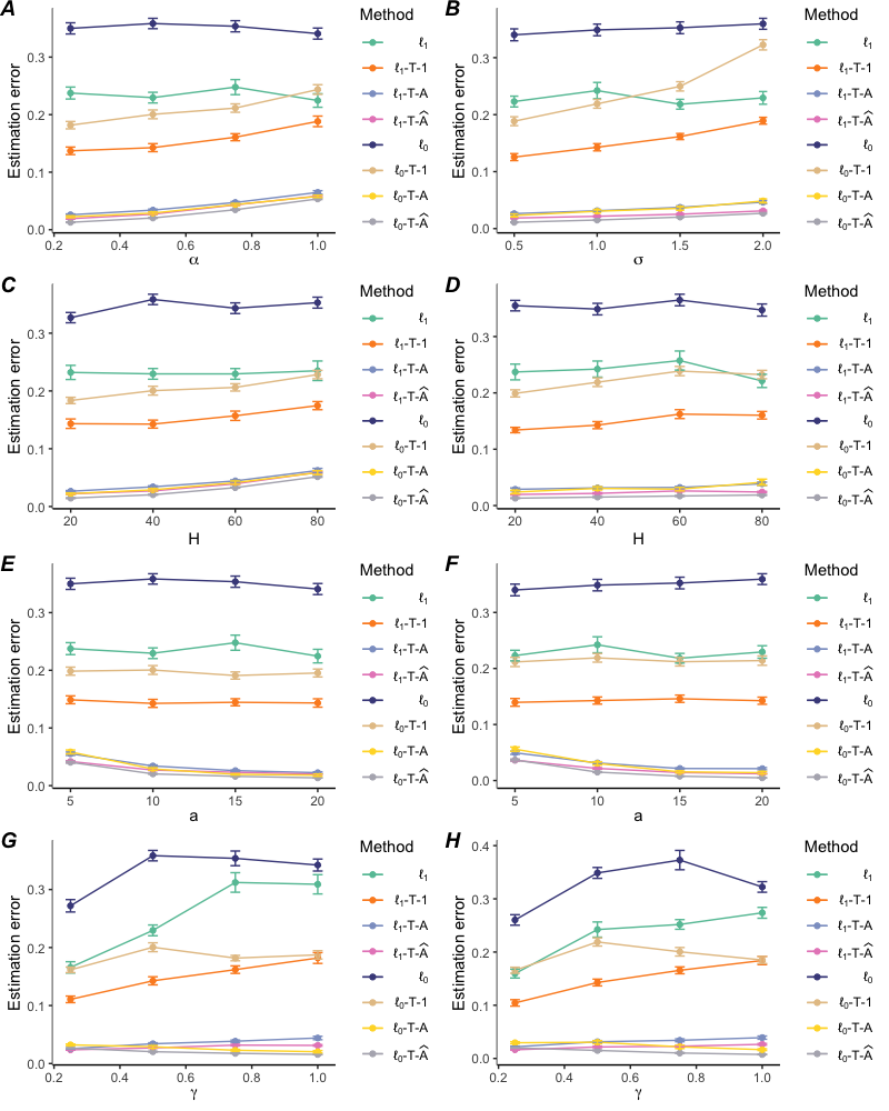
Figure 1: Estimation results in Scenario 1. From left to right: Configurations 1 and 2. From top to bottom: performances with varying discrepancy levels ($\alpha$ and $\sigma$), difference vector changing frequencies ($H$), cardinalities of the informative set ($a$) and change magnitudes ($\gamma$), respectively.

4.1.1 Simulation studies with varied source frequencies

To examine the performance of our proposed methods under varying source frequencies, we construct $10$ ordered sources, each associated with a unique observation frequency, i.e.

$$n_{k}=200\times(11-k),\quad k\in[10].$$ (28)

We vary the number of observed sources $K$ from $1$ to $10$ and depict in Figure 2 the following quantity:

$$K\times\mbox{the harmonic mean of source observations in }[K].$$ (29)

Let the target data be constructed as Scenario 1, with the parameter $\gamma=0.5$. For $k\in[K]$, let the $k$th source data follow Configuration 1 with the specified parameters $\mathcal{A}=[K]$, $H=0.2$ and $\alpha=0.5$. The estimators considered include multisource-transferred $\ell_{1}$- and $\ell_{0}$-penalised estimators which use

• all sources in $[K]$, i.e. (16) and (17), and

• a set of sources identified in the selection step, $\widetilde{\mathcal{A}}$, i.e. (26) with $\widehat{\mathcal{A}}=[K]$.

Evaluations and choices of tuning parameters remain the same as introduced before. The simulation results are depicted in Figure 2.

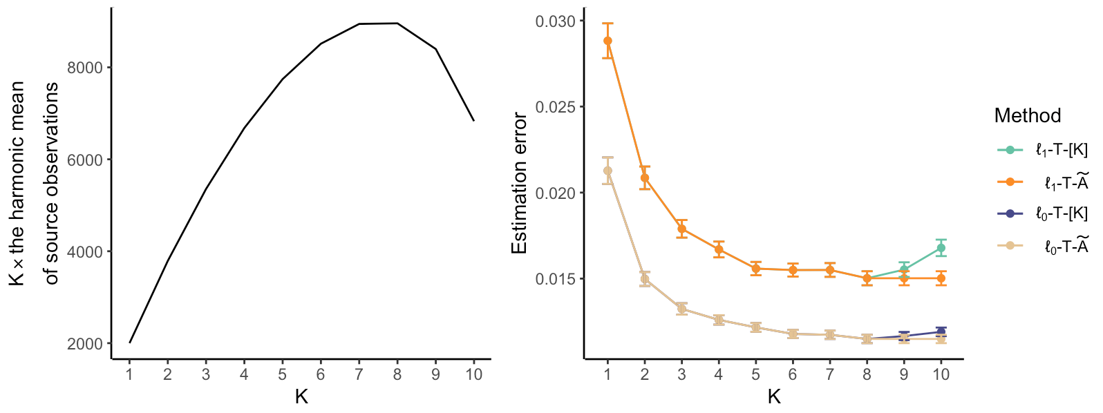
Figure 2: Results of Section 4.1.1. Left panel: Relationship between $K$ the number of sources and the quantity in (29), with sample sizes detailed in (28). Right panel: Estimation results as $K$ varies.

The left panel in Figure 2 shows that increasing the number of source datasets $K$ does not necessarily raise the value $K^{2}(\sum_{k\in[K]}{n_{k}}^{-1})^{-1}$, which is the denominator in the fluctuation term in our estimation error bounds. This observation aligns with the discussion in Section 3.2.1. We, again, highlight that our focus is not simply on increased the source sample sizes, but on increased source observation frequencies and guarantee adaptability to varying observation frequencies across multiple sources. The study by Cai et al. (2023) in the high-frequency functional data analysis assume a uniform observation across multisources, thus overlooking the interesting features we have noted.

From the right panel in Figure 2, we observe that transferred estimators using all sources in $[K]$ show a turning point at $K=8$. At this point, estimation errors transition from decreasing to increasing. This turning point matches the one in the left panel, where the term $K^{2}(\sum_{k\in[K]}{n_{k}}^{-1})^{-1}$ shifts from an increasing to decreasing trend. Comparing the performances of transferred estimators that utilise all sources to those with selected sources, we see that an additional source selection step, as shown in Section 3.2.1, ensures the precision of transferred estimators remains non-decreasing as the number of sources grows. In the varied source frequency framework, hence, simply adding more beneficial sources does not necessarily improve precision.

4.2 Real data analysis

Consider two real datasets: the U.S. electric power operations dataset (Independent Statistics and Analysis, 2023) and the air quality dataset (The World Air Quality Index project, 2023). All methods listed in Section 4.1 are considered, except those that incorporate known informative multisources. Tuning parameters involved are chosen following Section 4.1. To evaluate different estimators, we split the target dataset into training and test datasets. Estimators are derived using the training dataset, while the mean squared errors are computed using the test dataset.

The U.S. electric power operations dataset includes daily records of the electrical power demand of the various regions and sub-balancing authorities (sub-BAs) within the U.S. electricity market. Our study specifically focuses on the New York Independent System Operator (NYISO), which consists of $11$ distinct sub-regions: Capital, Central, Dunwoodie, Genesee, Hudson Valley, Long Island, Millwood, Mohawk Valley, New York City, North and West.

We conduct two separate analyses, using data collected every Saturday from 2nd July 2020 to 1st July 2023 ($156$ days) for New York City and Central sub-regions as the target datasets. For both analyses, daily observations from other sub-regions within the same time frame ($1092$ days) serve as source data. For transfer learning estimators utilising unisource data, the Dunwoodie sub-region is chosen when New York City is the target, due to their similar urban characteristics. For Central being the target, the Mohawk Valley sub-region is selected, given their geographical alignment. We split the target dataset into training and test datasets, with data from even-week Saturdays for training and odd-week for testing. Results are shown in Table 1.

Table 1 indicates that transfer learning methods, especially those using estimated informative multisources, outperform traditional methods when estimating electricity consumption in both target regions. This emphasises the advantage of leveraging source data to enhance estimation precision. It is worth mentioning that simply including all multisources without selection for transfer might not improve estimation performance. The results could even be worse than those obtained only using the target data. This highlights the necessity of the informative set detection algorithm, as shown in Algorithm 1. The estimated informative sets through Algorithm 1, consist of sub-regions with electricity consumption patterns similar to those of the target regions. For instance, when New York City is the target, the estimated informative set features Long Island, likely because of their shared urban characteristics and geographic proximity.

Table 1: Estimation results for New York City and Central sub-regions on the U.S. electric power operations dataset, and London and Paris on the air quality dataset. The reported values are mean squared errors.

Method	New York City	Central	Paris	London
$\ell_{1}$	0.3734	0.6390	0.9872	0.9872
$\ell_{1}$-T-1	0.1952	0.3026	0.9043	0.9179
$\ell_{1}$-T-$\widehat{\mathcal{A}}$	0.1955	0.2789	0.9139	0.8608
$\ell_{1}$-T-$[K]$	0.4586	0.4025	0.9205	0.9802
$\ell_{0}$	0.4558	0.7638	1.2649	0.9872
$\ell_{0}$-T-1	0.3052	0.4772	0.9134	0.9872
$\ell_{0}$-T-$\widehat{\mathcal{A}}$	0.2999	0.4731	0.8851	0.8860
$\ell_{0}$-T-$[K]$	0.5813	0.5624	0.9167	0.9916

The air quality dataset collects daily air quality measurements (e.g. $\text{PM}_{2.5}$, $\text{PM}_{10}$, $\text{O}_{3}$, $\text{NO}_{2}$ and CO) from various cities worldwide. As urban areas and industrial activities continue to grow, exploring these metrics becomes important for both policy-making and public health implications.

Two separate analyses are conducted on $\text{PM}_{2.5}$ data from every Saturday between 2nd July 2020 to 1st July 2023 ($156$ days), selecting Paris and London as the target datasets. For both analyses, daily $\text{PM}_{2.5}$ measurements from $17$ different cities (Amsterdam, Bangkok, Beijing, Chongqing, Dalian, Hamburg, Harbin, Hefei, Hong Kong, Kunming, Los Angeles, Sanya, Seoul, Shanghai, Singapore, Tianjin and Xi’an) within the same duration ($1,092$ days) serve as the multisource data. For transfer learning estimators utilising unisource data, Paris is selected as the source for London and vice versa, due to their geographical proximity and similar urban structures. The target dataset is split into training (even-week Saturdays) and test datasets (odd-week Saturdays). Results can be found in Table 1.

Similar observations and conclusions as those from the previous dataset can be drawn, demonstrating the superiority of transfer learning methods especially when using informative multisources for transfer. Furthermore, the estimated informative sets from Algorithm 1 present interesting city-to-city connections. For instance, data from Paris share the same patterns with those from the cities including Beijing, Hong Kong, Kunming and London, suggesting common pollution patterns. London’s air quality patterns resonate closely with those of Amsterdam, Beijing, Paris and Singapore. These interconnected trends not only highlight the similarities between these cities but also suggest collaborative strategies and interventions to address air quality issues.

5 Conclusions

In this paper, we study transfer learning for the estimation of piecewise-constant signals, which is the first time seen in the literature. Our approaches leverage higher observation frequencies and accommodate diverse observation frequencies across multiple sources. We consider both $\ell_{1}$- and $\ell_{0}$-penalisation. The theoretical advantages of the transferred $\ell_{0}$-penalized estimator include its independence from the minimum length condition and its reduced reliance on unknown parameters when selecting tuning parameters, compared to its $\ell_{1}$-penalised counterpart.

The current work offers several interesting directions for future studies. Firstly, the foundational frameworks and methodologies used for the source and target models in this study can be generalised to transfer learning for piecewise-polynomial mean estimation. Specifically, we can investigate the trend filtering method (e.g. Tibshirani, 2014; Ortelli and van de Geer, 2019; Guntuboyina et al., 2020), which incorporates the $r$th order difference operator $D^{(r)}$, a generalisation of the difference operator $D$ in (4). The associated challenges lie in the extension of the alignment operator $P^{n_{k},n_{0}}$, defined in (5), and the characterisation of its associated eigenvalue spectrum, like Lemma 8. Secondly, an extension to transfer learning for high-dimensional linear regression models with general designs and piecewise-constant regression coefficients (Wang et al., 2022; Xu and Fan, 2019), can be studied. The main challenges are to establish measures for the discrepancies between the source and the target regression coefficients and the covariance matrices of their respective covariates.

Appendices

All technical details of this paper can be found in the Appendices. The proofs of Theorem 1, Theorem 2 and the theoretical results in Section 3 are presented in Appendices A, B and C, respectively. Details and results in Section 4 are collected in Appendix D.

Appendix A Proof of Theorem 1

The proof of Theorem 1 can be found in Section A.2. Relevant notation is provided in Section A.1 and all necessary auxiliary results are in Section A.3.

A.1 Additional notation

Let us consider $\mathcal{S}\subseteq[n_{0}-1]$ as defined in (2) with cardinality $s_{0}$. When $s_{0}>0$, denote $\mathcal{S}=\{t_{1},\dots,t_{s_{0}}\}$ and let the sign vector $q\in\mathbb{R}^{s_{0}}$ be defined as

$$q_{i}=\mathrm{sign}\big{(}(Df)_{t_{i}}\big{)},\quad\mbox{for each }i\in[s_{0}]$$ (30)

with $D$ defined in (4), and the set $\mathcal{S}_{\pm}\subseteq[s_{0}+1]$ be defined as

$$\mathcal{S}_{\pm}=\{i\in\{2,\dots,s_{0}\}\colon q_{i}q_{i-1}=-1\}\cup\{1,s_{0}+1\}.$$ (31)

Using the difference operator $D$ defined in (4), if $s_{0}<n_{0}-1$, let $\Psi^{-\mathcal{S}}\in\mathbb{R}^{n_{0}\times(n_{0}-1-s_{0})}$ be defined as

$$\Psi^{-\mathcal{S}}=D_{-\mathcal{S}}^{\top}(D_{-\mathcal{S}}D_{-\mathcal{S}}^{\top})^{-1},$$ (32)

which, as investigated by Ortelli and van de Geer (2019), is well-defined.

We then introduce the definition of effective sparsity for target signals $f$, as proposed by Ortelli and van de Geer (2019). This can be seen as a substitute for sparsity and then can be used to establish upper bounds.

Definition 1 (Effective sparsity).

Let the set $\mathcal{S}\subseteq[n_{0}-1]$ with cardinality $s_{0}$ be defined in (2). If $s_{0}>0$, let the sign vector $q\in\mathbb{R}^{s_{0}}$ be defined in (30). The effective sparsity of target signals $f$, denoted as $\Gamma_{\mathcal{S}}^{2}$, is defined as

$$\Gamma_{\mathcal{S}}^{2}=\begin{cases}\big{\{}\max\big{\{}\sum_{j=1}^{n_{0}-1-s_{0}}\big{|}\big{(}1-w^{-\mathcal{S}}_{j}\big{)}\big{(}(D\theta)_{-\mathcal{S}}\big{)}_{j}\big{|}\colon\|\theta\|_{1/n_{0}}=1\big{\}}\big{\}}^{2},&\mbox{if }s_{0}=0,\\ \big{\{}\max\big{\{}q^{\top}(D\theta)_{\mathcal{S}}\colon\|\theta\|_{1/n_{0}}=1\big{\}}\big{\}}^{2},&\mbox{if }s_{0}=n_{0}-1,\\ \big{\{}\max\big{\{}q^{\top}(D\theta)_{\mathcal{S}}-\sum_{j=1}^{n_{0}-1-s_{0}}\big{|}\big{(}1-w^{-\mathcal{S}}_{j}\big{)}\big{(}(D\theta)_{-\mathcal{S}}\big{)}_{j}\big{|}\colon\|\theta\|_{1/n_{0}}=1\big{\}}\big{\}}^{2},&\mbox{otherwise}.\end{cases}$$

Here, if $s_{0}<n_{0}-1$, the vector $w^{-\mathcal{S}}\in[0,1]^{n_{0}-1-s_{0}}$ is defined as

$$w^{-\mathcal{S}}_{j}=\Big{\|}\Psi^{-\mathcal{S}}_{,j}\Big{\|}_{1/n_{0}}\Big{(}\max_{j\in[n_{0}-1-s_{0}]}\Big{\|}\Psi^{-\mathcal{S}}_{,j}\Big{\|}_{1/n_{0}}\Big{)}^{-1},\quad j\in[n_{0}-1-s_{0}],$$

with $j$th column of $\Psi^{-\mathcal{S}}$ denoted as $\Psi^{-\mathcal{S}}_{,j}$.

A.2 Proof of Theorem 1

Proof of Theorem 1.

This proof consists of four steps. In Step 1, we decompose our target quantity into several terms. In Step 2 and Step 3, we deal with these terms separately. In Step 4, we gather all the pieces and complete the proof.

Step 1. It directly follows from the definition of $\widehat{f}$ that

$$\frac{1}{2n_{0}}\big{\|}P^{n_{0},n_{1}}y^{(1)}-\widehat{f}\big{\|}_{2}^{2}+\lambda\|D\widehat{f}\|_{1}\leq\frac{1}{2n_{0}}\big{\|}P^{n_{0},n_{1}}y^{(1)}-f\big{\|}_{2}^{2}+\lambda\|Df\|_{1}.$$

Given that $y^{(1)}=f^{(1)}+\epsilon^{(1)}$ with $f^{(1)}=P^{n_{1},n_{0}}f+\delta$, we obtain that

$$\frac{1}{2n_{0}}\big{\|}\widehat{f}-P^{n_{0},n_{1}}P^{n_{1},n_{0}}f\big{\|}_{2}^{2}\leq \frac{1}{2n_{0}}\big{\|}f-P^{n_{0},n_{1}}P^{n_{1},n_{0}}f\big{\|}_{2}^{2}+\frac{1}{n_{0}}\widetilde{\epsilon}^{\top}\big{(}\widehat{f}-f\big{)}+\lambda\|Df\|_{1}$$

$$\hskip 14.22636pt-\lambda\|D\widehat{f}\|_{1}+\frac{1}{n_{0}}\big{(}P^{n_{0},n_{1}}\delta\big{)}^{\top}\big{(}\widehat{f}-f\big{)},$$

with $\widetilde{\epsilon}=P^{n_{0},n_{1}}\epsilon^{(1)}\in\mathbb{R}^{n_{0}}$. By Lemma 8, it holds that

$$\frac{1}{2n_{0}}\big{\|}\widehat{f}-f\big{\|}_{2}^{2}\leq \frac{1}{n_{0}}\widetilde{\epsilon}^{\top}\big{(}\widehat{f}-f\big{)}+\lambda\left\|Df\right\|_{1}-\lambda\|D\widehat{f}\|_{1}+\frac{1}{n_{0}}\big{(}P^{n_{0},n_{1}}\delta\big{)}^{\top}\big{(}\widehat{f}-f\big{)}$$

$$= (I.1)+(I.2)+(I.3)+(II)=(I)+(II).$$ (33)

Step 2. In this step, we deal with the term $(I)$ in (A.2). We claim that if

$$\lambda=C_{\lambda}\big{(}n_{\max}^{(0)}/(n_{1}n_{0})\big{)}^{1/2},$$ (34)

with $n_{\max}^{(0)}$ defined in 1 and an absolute constant $C_{\lambda}>0$, then it holds that

$$\mathbb{P}\Bigg{\{}(I)\leq \frac{3}{8n_{0}}\big{\|}\widehat{f}-f\big{\|}_{2}^{2}+C_{\mathcal{E}}\frac{n_{\max}^{(0)}/\widetilde{n}_{\min}^{(0)}(s_{0}+1)\big{(}1+\log(n_{\max}^{(0)})\big{)}}{n_{1}}\Bigg{\}}\geq 1-n_{0}^{-c_{\mathcal{E}}},$$ (35)

with $\widetilde{n}_{\min}^{(0)}$ defined in Remark 1 and absolute constants $C_{\mathcal{E}},c_{\mathcal{E}}>0$. Then we prove this claim under two scenarios $s_{0}=n_{0}-1$ and $s_{0}<n_{0}-1$ in Step 2.1 and Step 2.2., respectively. Before proving the claim, note that by the definition of the alignment operator $P^{n_{0},n_{1}}$ in (5) with the assumption that $n_{1}\geq 2n_{0}$, we have that for any $i\in n_{0}$,

$$\widetilde{\epsilon}_{i}=\big{(}P^{n_{0},n_{1}}\epsilon^{(1)}\big{)}_{i}=\frac{1}{\lceil i(n_{1}/n_{0})\rceil-\lceil(i-1)(n_{1}/n_{0})\rceil}\sum_{j=\lceil(i-1)(n_{1}/n_{0})\rceil+1}^{\lceil i(n_{1}/n_{0})\rceil}\epsilon^{(1)}_{j}.$$

Since for each $i\in[n_{0}]$, there is no overlapping of independent random variables $\{\epsilon^{(1)}_{j}\}_{j=1}^{n_{1}}$, we have that $\{\widetilde{\epsilon}_{i}\}_{i=1}^{n_{0}}$ are independent. According to Proposition 2.6.1 in Vershynin (2018), we derive that

$$\{\widetilde{\epsilon}_{i}\}_{i=1}^{n_{0}}\sim\mbox{mean-zero }C_{\sigma}\big{(}\lceil i(n_{1}/n_{0})\rceil-\lceil(i-1)(n_{1}/n_{0})\rceil\big{)}^{-1/2}\mbox{-sub-Gaussian}.$$

Since

$$\big{(}\lceil i(n_{1}/n_{0})\rceil-\lceil(i-1)(n_{1}/n_{0})\rceil\big{)}^{-1/2}\leq(\lceil n_{1}/n_{0}\rceil-1)^{-1/2}\leq\big{(}n_{0}/(n_{1}-n_{0})\big{)}^{1/2}\leq\big{(}2n_{0}/n_{1}\big{)}^{1/2},$$

where the final inequality follows from the assumption $n_{1}/n_{0}\geq 2$, we can conclude that

$$\widetilde{\epsilon}_{i}\overset{ind.}{\sim}\mbox{mean-zero }C_{\sigma}\big{(}2n_{0}/n_{1}\big{)}^{1/2}\mbox{-sub-Gaussian}.$$ (36)

Step 2.1. In this step, we prove the claim stated in (35) when $s_{0}=n_{0}-1$. By (36) and general Hoeffding inequality (e.g. Theorem 2.6.3 in Vershynin, 2018), we can conclude that there exists an absolute constant $c_{0}>0$ such that

$$\mathbb{P}\big{\{}\mathcal{E}_{1}\big{\}}\geq 1-\exp\{-c_{0}n_{0}\}\quad\mbox{with}\quad\mathcal{E}_{1}=\big{\{}(I)\leq n_{1}^{-1/2}\big{\|}\widehat{f}-f\big{\|}_{2}+\lambda\|Df\|_{1}-\lambda\|D\widehat{f}\|_{1}\big{\}}.$$ (37)

From now on we assume that the event $\mathcal{E}_{1}$ holds in this sub-step. By applying Cauchy–Schwartz inequality and the fact that $|ab|\leq a^{2}+b^{2}/4$, we obtain that

$$(I)\leq\frac{1}{4n_{0}}\big{\|}\widehat{f}-f\big{\|}_{2}^{2}+\frac{n_{0}}{n_{1}}+\lambda\left\|Df\right\|_{1}-\lambda\|D.\widehat{f}\|_{1}.$$ (38)

Note that with the sign vector $q\in\mathbb{R}^{s_{0}}$ defined in (30), we have that

$$\|Df\|_{1}=\big{\|}(Df)_{\mathcal{S}}\big{\|}_{1}=q^{\top}(Df)_{\mathcal{S}}\quad\mbox{and}\quad\|D\widehat{f}\|_{1}=\big{\|}(D\widehat{f})_{\mathcal{S}}\big{\|}_{1}\geq q^{\top}(D\widehat{f})_{\mathcal{S}}.$$ (39)

Combining (38) and (39), we have that

$$(I)\leq \frac{1}{4n_{0}}\big{\|}\widehat{f}-f\big{\|}_{2}^{2}+\frac{n_{0}}{n_{1}}+\lambda q^{\top}\big{(}D(f-\widehat{f})\big{)}_{\mathcal{S}}\leq\frac{1}{4n_{0}}\big{\|}\widehat{f}-f\big{\|}_{2}^{2}+\frac{n_{0}}{n_{1}}+\lambda\Gamma_{\mathcal{S}}\big{\|}\widehat{f}-f\big{\|}_{1/n_{0}}$$

$$\leq \frac{3}{8n_{0}}\big{\|}\widehat{f}-f\big{\|}_{2}^{2}+\frac{n_{0}}{n_{1}}+2\lambda^{2}\Gamma_{\mathcal{S}}^{2}\leq\frac{3}{8n_{0}}\big{\|}\widehat{f}-f\big{\|}_{2}^{2}+\big{(}C_{\lambda}^{2}C_{\Gamma}+1\big{)}\frac{(s_{0}+1)}{n_{1}},$$ (40)

where

• the second inequality is derived from the definition of the effective sparsity $\Gamma_{\mathcal{S}}$ in Definition 1,

• the third inequality is based on the fact that $|ab|\leq 2a^{2}+b^{2}/8$,

• and the final inequality arises from the choice of $\lambda$ in (34), Lemma 11 and for any $i\in[s_{0}+1]$, $n_{i}^{(0)}=1$ and $n_{\max}^{(0)}=1$.

Since when $s_{0}=n_{0}-1$, we have $\widetilde{n}_{\min}^{(0)}=n_{\max}^{(0)}=1$, then combining (37) and (A.2), it holds with an absolute constant $c_{1}>0$ that

$$\mathbb{P}\Bigg{\{}(I)\leq \frac{3}{8n_{0}}\big{\|}\widehat{f}-f\big{\|}_{2}^{2}+\big{(}C_{\lambda}^{2}C_{\Gamma}+1\big{)}\frac{n_{\max}^{(0)}/\widetilde{n}_{\min}^{(0)}(s_{0}+1)\big{(}1+\log(n_{\max}^{(0)})\big{)}}{n_{1}}\Bigg{\}}\geq 1-n_{0}^{-c_{1}},$$

which proves (35) when $s_{0}=n_{0}-1$.

Step 2.2. In this step, we prove the claim stated in (35) when $s_{0}<n_{0}-1$.

By (36) and Theorem 9, we obtain that $\mathbb{P}\{\mathcal{E}_{2}\}\geq 1-\exp\big{\{}-c_{2}(s_{0}+1)\log\big{(}n_{0}/(s_{0}+1)\big{)}\big{\}}$ with

$$\mathcal{E}_{2}=\Bigg{\{}(I.1)\leq \frac{1}{4n_{0}}\big{\|}\widehat{f}-f\big{\|}_{2}^{2}+C_{2}\frac{(s_{0}+1)\log(n_{\max}^{(0)})}{n_{1}}+\lambda\sum_{i=1}^{n_{0}-1-s_{0}}\big{|}w^{-\mathcal{S}}_{i}\big{(}(D\widehat{f}-Df)_{-\mathcal{S}}\big{)}_{i}\big{|}\Bigg{\}},$$

where $n_{\max}^{(0)}$ is defined in 1 and $C_{2},c_{2}>0$ are absolute constants, if $\lambda$ satisfies

$$\lambda\geq\lambda_{\mathcal{S}}\quad\mbox{with}\quad\lambda_{\mathcal{S}}=C_{\lambda_{0}}\max_{j\in[n_{0}-1-s_{0}]}\left\|\Psi^{-\mathcal{S}}_{,j}\right\|_{1/n_{0}}n_{1}^{-1/2}\leq C_{\lambda_{0}}\sqrt{\frac{n_{\max}^{(0)}}{2n_{1}n_{0}}},$$ (41)

where the last inequality follows from Lemma 10 and $C_{\lambda_{0}}>0$ is an absolute constant. Note that the function

$$s\mapsto-c_{2}(s+1)\log(n_{0}/(s+1)))$$

is convex, so its maximum over $\{0\}\cup[n_{0}-2]$ is attained at either $s=0$ or $s=n_{0}-2$. Thus, it holds with an absolute constant $c_{3}>0$ that

$$\mathbb{P}\{\mathcal{E}_{2}\}\geq 1-\max\big{\{}\exp\{-c_{2}\log(n_{0})\},\exp\{-c_{2}(n_{0}-1)\log(n_{0}/(n_{0}-1))\}\big{\}}\geq 1-n_{0}^{-c_{3}}.$$ (42)

From now on we assume that the event $\mathcal{E}_{2}$ holds in this sub-step. Note that

$$\lambda\sum_{i=1}^{n_{0}-1-s_{0}}\big{|}w^{-\mathcal{S}}_{i}\big{(}(D\widehat{f}-Df)_{-\mathcal{S}}\big{)}_{i}\big{|}+\lambda\|Df\|_{1}-\lambda\|D\widehat{f}\|_{1}$$

$$= -\lambda\sum_{i=1}^{n_{0}-1-s_{0}}\big{(}1-w^{-\mathcal{S}}_{i}\big{)}\big{|}\big{(}(D\widehat{f}-Df)_{-\mathcal{S}}\big{)}_{i}\big{|}+\lambda\big{\|}(D\widehat{f}-Df)_{-\mathcal{S}}\big{\|}_{1}+\lambda\|Df\|_{1}-\lambda\|D\widehat{f}\|_{1}$$

$$\leq -\lambda\sum_{i=1}^{n_{0}-1-s_{0}}\big{(}1-w^{-\mathcal{S}}_{i}\big{)}\big{|}\big{(}(D\widehat{f}-Df)_{-\mathcal{S}}\big{)}_{i}\big{|}+\lambda\big{\|}(Df)_{\mathcal{S}}\|_{1}-\lambda\big{\|}(D\widehat{f})_{\mathcal{S}}\|_{1}+2\lambda\big{\|}(Df)_{-\mathcal{S}}\big{\|}_{1}$$

$$\leq -\lambda\sum_{i=1}^{n_{0}-1-s_{0}}\big{(}1-w^{-\mathcal{S}}_{i}\big{)}\big{|}\big{(}(D\widehat{f}-Df)_{-\mathcal{S}}\big{)}_{i}\big{|}+\lambda q^{\top}\big{(}D(f-\widehat{f})_{\mathcal{S}}\big{)}+2\lambda\big{\|}(Df)_{-\mathcal{S}}\big{\|}_{1}$$

$$\leq \lambda\Gamma_{\mathcal{S}}\big{\|}\widehat{f}-f\big{\|}_{1/n_{0}}+2\lambda\big{\|}(Df)_{-\mathcal{S}}\big{\|}_{1}\leq\frac{1}{8n_{0}}\big{\|}\widehat{f}-f\big{\|}_{2}^{2}+2\lambda^{2}\Gamma_{\mathcal{S}}^{2}+2\lambda\big{\|}(Df)_{-\mathcal{S}}\big{\|}_{1},$$ (43)

where

• the first equality follows from the fact that $w^{-\mathcal{S}}\in[0,1]^{n_{0}-1-s_{0}}$ defined in Definition 1,

• the first inequality follows from the reverse triangle inequality,

• the second inequality follows from the fact that $\big{\|}(Df)_{\mathcal{S}}\big{\|}_{1}=q^{\top}(Df)_{\mathcal{S}}$ and $\big{\|}(D\widehat{f})_{\mathcal{S}}\big{\|}_{1}\geq q^{\top}(D\widehat{f})_{\mathcal{S}}$. Specifically, the sign vector $q$ is defined in (30) when $s_{0}>0$ and is set to $q=0$ for $s_{0}=0$,

• the third inequality follows from the definition of the effective sparsity $\Gamma_{\mathcal{S}}$ in Definition 1,

• the final inequality follows from the fact $|ab|\leq 2a^{2}+b^{2}/8$.

By the construction of $\mathcal{S}$ in (2), it holds that

$$\left\|\left(Df\right)_{-\mathcal{S}}\right\|_{1}=0.$$ (44)

By Lemma 11, we obtain a deterministic result with an absolute constant $C_{\Gamma}>0$ as follows

$$\Gamma_{\mathcal{S}}^{2}\leq\begin{cases}C_{\Gamma}\log(n_{0}),\quad&\mbox{if }s_{0}=0,\\ C_{\Gamma}n_{0}\left(\sum_{i\in\mathcal{S}_{\pm}}\frac{1+\log(n^{(0)}_{i})}{n^{(0)}_{i}}+\sum_{i\in S\setminus\mathcal{S}_{\pm}}\frac{1+\log(n^{(0))}_{i})}{n^{(0)}_{\max}}\right),\quad&\mbox{otherwise}.\end{cases}$$

Then it holds with $n_{\max}^{(0)}$ and $\widetilde{n}_{\min}^{(0)}$ defined in 1 and Remark 1, respectively, that

$$\Gamma_{\mathcal{S}}^{2}\leq C_{\Gamma}\frac{n_{0}(s_{0}+1)\big{(}1+\log(n_{\max}^{(0)})\big{)}}{\widetilde{n}_{\min}^{(0)}}.$$ (45)

Then combining (42), (A.2), (44) and (45), with $n_{\max}^{(0)}\geq n_{0}/(s_{0}+1)$ and the choice of $\lambda$ in (34) which satisfies (41), it holds with an absolute constant $C_{3}>0$ that

$$\mathbb{P}\Bigg{\{}(I)\leq \frac{3}{8n_{0}}\big{\|}\widehat{f}-f\big{\|}_{2}^{2}+C_{3}\frac{n_{\max}^{(0)}/\widetilde{n}_{\min}^{(0)}(s_{0}+1)\big{(}1+\log(n_{\max}^{(0)})\big{)}}{n_{1}}\Bigg{\}}\geq 1-n_{0}^{-c_{3}},$$

which proves (35) when $s_{0}<n_{0}-1$.

Step 3. We consider the term $(II)$ in (A.2). Note that by applying the Cauchy-Schwartz inequality and utilising the fact that $|ab|\leq 4a^{2}+b^{2}/16$, we can establish that

$$(II)\leq \frac{4\|P^{n_{0},n_{1}}\delta\|_{2}^{2}}{n_{0}}+\frac{1}{16n_{0}}\big{\|}\widehat{f}-f\big{\|}_{2}^{2}\leq\frac{4\|\delta\|_{2}^{2}}{n_{0}\big{(}\lceil n_{1}/n_{0}\rceil-1\big{)}}+\frac{1}{16n_{0}}\big{\|}\widehat{f}-f\big{\|}_{2}^{2}$$

$$\leq \frac{8\|\delta\|_{2}^{2}}{n_{1}}+\frac{1}{16n_{0}}\big{\|}\widehat{f}-f\big{\|}_{2}^{2},$$ (46)

where the second inequality follows from Lemma 8 and the final inequality follows from the assumption that $n_{1}\geq 2n_{0}$.

Step 4. Choosing $\lambda$ as (34), and combining (A.2), (35) and (A.2), we have with an absolute constant $C_{4}>0$ that

$$\mathbb{P}\Bigg{\{}\big{\|}\widehat{f}-f\big{\|}_{1/n_{0}}^{2}\leq C_{4}\frac{n_{\max}^{(0)}/\widetilde{n}_{\min}^{(0)}(s_{0}+1)\big{(}1+\log(n_{\max}^{(0)})\big{)}+\|\delta\|_{2}^{2}}{n_{1}}\Bigg{\}}\geq 1-n_{0}^{-c_{\mathcal{E}}}.$$

Under 1, if $\lambda=C_{\lambda}\big{(}(s_{0}+1)n_{1}\big{)}^{-1/2}$, then it holds with an absolute constant $C_{5}>0$ that

$$\mathbb{P}\Bigg{\{}\big{\|}\widehat{f}-f\big{\|}_{1/n_{0}}^{2}\leq C_{5}\frac{(s_{0}+1)\big{\{}1+\log\big{(}n_{0}/(s_{0}+1)\big{)}\big{\}}+\|\delta\|_{2}^{2}}{n_{1}}\Bigg{\}}\geq 1-n_{0}^{-c_{\mathcal{E}}},$$

completing the proof. ∎

A.3 Additional lemmas

Lemma 8.

For any $n,m\in\mathbb{N}^{*}$, let the alignment operator $P^{n,m}\in\mathbb{R}^{n\times m}$ be defined in (5). If $n\geq m$ then we have that

$$\sqrt{\lceil n/m\rceil-1}\leq\sigma_{m}\left(P^{n,m}\right)\leq\sigma_{1}\left(P^{n,m}\right)\leq\sqrt{\lceil n/m\rceil}.$$ (47)

Conversely, if $m>n$, then

$$\big{(}\lceil m/n\rceil\big{)}^{-1/2}\leq\sigma_{n}\left(P^{n,m}\right)\leq\sigma_{1}\left(P^{n,m}\right)\leq\big{(}\lceil m/n\rceil-1\big{)}^{-1/2}.$$ (48)

and $P^{n,m}P^{m,n}=I_{n}$.

Proof.

We first consider the scenario where $n\geq m$. Based on the definition of $P^{n,m}$ in (5), for any $i,j\in[m]$, we have that

$$\big{(}(P^{n,m})^{\top}P^{n,m}\big{)}_{i,j}= \sum_{l=1}^{n}\mathbbm{1}_{\left\{\lceil(i-1)n/m\rceil+1\leq l\leq\lceil in/m\rceil\right\}}\mathbbm{1}_{\left\{\lceil(j-1)n/m\rceil+1\leq l\leq\lceil jn/m\rceil\right\}}$$

$$= \begin{cases}\lceil jn/m\rceil-\lceil(j-1)n/m\rceil,&\mbox{if }i=j,\\ 0,&\mbox{otherwise},\end{cases}$$

where the second equality follows from that there is no overlapping of non-zero entries among the columns of $P^{n,m}$. Since for any $j\in[m]$,

$$\lceil(j-1)n/m\rceil+\lceil n/m\rceil-1\leq\lceil jn/m\rceil\leq\lceil(j-1)n/m\rceil+\lceil n/m\rceil,$$

it holds with $\lambda_{1}\big{(}(P^{n,m})^{\top}P^{n,m}\big{)}\geq\cdots\geq\lambda_{m}\big{(}(P^{n,m})^{\top}P^{n,m}\big{)})$ being the eigenvalues of $(P^{n,m})^{\top}P^{n,m}$ that

$$\lceil n/m\rceil-1\leq\lambda_{m}\big{(}(P^{n,m})^{\top}P^{n,m}\big{)}\leq\lambda_{1}\big{(}P^{n,m})^{\top}P^{n,m}\big{)}\leq\lceil n/m\rceil,$$

which proves (47).

Next, we consider the scenario where $m>n$. By the definition of $P^{n,m}$ in (5), we have that for any $i,j\in[n]$,

$$\big{(}P^{n,m}(P^{n,m})^{\top}\big{)}_{i,j}= \sum_{l=1}^{m}\frac{\mathbbm{1}_{\left\{\lceil(i-1)m/n\rceil+1\leq l\leq\lceil im/n\rceil\right\}}}{\lceil im/n\rceil-\lceil(i-1)m/n\rceil}\frac{\mathbbm{1}_{\left\{\lceil(j-1)m/n\rceil+1\leq l\leq\lceil jm/n\rceil\right\}}}{\lceil jm/n\rceil-\lceil(j-1)m/n\rceil}$$

$$= \begin{cases}\big{(}\lceil jm/n\rceil-\lceil(j-1)m/n\rceil\big{)}^{-1},&\mbox{if }i=j,\\ 0,&\mbox{otherwise},\end{cases}$$

where the second equality is based on the fact that there is no overlapping of non-zero entries among the rows of $P^{n,m}$. Since

$$\lceil(j-1)m/n\rceil+\lceil m/n\rceil-1\leq\lceil jm/n\rceil\leq\lceil(j-1)m/n\rceil+\lceil m/n\rceil,$$

it holds $\lambda_{1}\big{(}P^{n,m}(P^{n,m})^{\top}\big{)}\geq\cdots\geq\lambda_{n}\big{(}P^{n,m}(P^{n,m})^{\top}\big{)}$ being the eigenvalues of $P^{n,m}(P^{n,m})^{\top}$ that

$$\big{(}\lceil m/n\rceil\big{)}^{-1}\leq\lambda_{n}\big{(}P^{n,m}(P^{n,m})^{\top}\big{)}\leq\lambda_{1}\big{(}P^{n,m}(P^{n,m})^{\top}\big{)}\leq\big{(}\lceil m/n\rceil-1\big{)}^{-1},$$

which proves (48). Additionally, by the definition of $P^{n,m}$ and $P^{m,n}$ in (5) under the assumption $m>n$, it holds that for ang $i,j\in[n]$

$$\big{(}P^{n,m}P^{m,n}\big{)}_{i,j} =\sum_{l=1}^{m}\frac{\mathbbm{1}_{\left\{\lceil(i-1)m/n\rceil+1\leq l\leq\lceil im/n\rceil\right\}}}{\lceil im/n\rceil-\lceil(i-1)m/n\rceil}\mathbbm{1}_{\left\{\lceil(j-1)m/n\rceil+1\leq l\leq\lceil jm/n\rceil\right\}}$$

$$= \begin{cases}1,&\mbox{if }i=j,\\ 0,&\mbox{otherwise},\end{cases}$$

which proves $P^{n,m}P^{m,n}=I_{n}$. ∎

Theorem 9 (van de Geer, 2020).

Let $\mathcal{S}\subseteq[n_{0}-1]$ be defined in (2) with cardinality $s_{0}$. Assume that $s_{0}<n_{0}-1$, then let $n_{\max}^{(0)}$, the matrix $\Psi^{-\mathcal{S}}\in\mathbb{R}^{n_{0}\times(n_{0}-1-s_{0})}$ and the vector $w^{-\mathcal{S}}\in\mathbb{R}^{n_{0}-1-s_{0}}$ be defined in 1, (32) and Definition 1, respectively. Furthermore, assume that $\{\widetilde{\epsilon}_{i}\}_{i=1}^{n_{0}}$ are independent mean-zero $\sigma$-sub-Gaussian variables. If there exists $\lambda$ satisfies

$$\lambda\geq\lambda_{\mathcal{S}}\quad\mbox{with}\quad\lambda_{\mathcal{S}}=C_{\lambda_{\mathcal{S}}}\sigma\max_{j\in[n_{0}-1-s_{0}]}\Big{\|}\Psi^{-\mathcal{S}}_{,j}\Big{\|}_{1/n_{0}}n_{0}^{-1/2},$$

with the $j$th column of $\Psi^{-\mathcal{S}}$ denoted as $\Psi^{-\mathcal{S}}_{,j}$ and an absolute constant $C_{\lambda_{\mathcal{S}}}>0$, then it holds with probability at least $1-\exp\big{\{}-c_{\epsilon}(s_{0}+1)\log\big{(}n_{0}/(s_{0}+1)\big{)}\big{\}}$ that

$$\frac{\widetilde{\epsilon}^{\top}\theta}{n_{0}}\leq \frac{1}{4n_{0}}\|\theta\|_{2}^{2}+C_{\epsilon}\sigma^{2}\frac{(s_{0}+1)\log(n_{\max}^{(0}))}{n_{0}}+\lambda\sum_{i=1}^{n_{0}-1-s_{0}}\big{|}w^{-\mathcal{S}}_{i}\big{(}(D\theta)_{-\mathcal{S}}\big{)}_{i}\big{|},$$

for any $\theta\in R^{n_{0}}$.

Lemma 10 (Ortelli and van de Geer, 2019).

Let $\mathcal{S}\subseteq[n_{0}-1]$ be defined in (2) with cardinality $s_{0}$. Assume that $s_{0}<n_{0}-1$, then let $\Psi^{-\mathcal{S}}$ and $n_{\max}^{(0)}$ be defined in (32) and 1, respectively. Denote the $j$th column of $\Psi^{-\mathcal{S}}$ as $\Psi^{-\mathcal{S}}_{,j}$, then it holds that

$$\max_{j\in[n_{0}-1-s]}\Big{\|}\Psi^{-\mathcal{S}}_{,j}\Big{\|}_{1/n_{0}}^{2}\leq\frac{n_{\max}^{(0)}}{2n_{0}}.$$

Lemma 11 (van de Geer, 2020).

Let $\mathcal{S}\subseteq[n_{0}-1]$ be defined in (2) with cardinality $s_{0}$ and effective sparsity $\Gamma_{\mathcal{S}}^{2}$ be defined in Definition 1. For $s_{0}>0$, let $\{n_{i}^{(0)}\}_{i=1}^{s_{0}+1}$, $n_{\max}^{(0)}$ and $\mathcal{S}_{\pm}$ be defined in 1 and Equation 31. It holds that

$$\Gamma_{\mathcal{S}}^{2}\leq\begin{cases}C_{\Gamma}\log(n_{0})\quad&\mbox{if }s_{0}=0,\\ C_{\Gamma}n_{0}\Big{(}\sum_{i\in\mathcal{S}_{\pm}}\frac{1+\log(n^{(0)}_{i})}{n^{(0)}_{i}}+\sum_{i\in\mathcal{S}\setminus\mathcal{S}_{\pm}}\frac{1+\log(n_{i}^{(0)})}{n_{\max}^{(0)}}\Big{)},\quad&\mbox{otherwise},\end{cases}$$

where $C_{\Gamma}>0$ is an absolute constant .

Appendix B Proof of Theorem 2

The proof of Theorem 2 can be found in Section B.1 with the necessary auxiliary results in Section B.2.

B.1 Proof of Theorem 2

Proof of Theorem 2.

This proof consists of four steps. In Step 1, we decompose our target quantity into several terms. We then deal with these terms individually in Step 2 and Step 3. In Step 4, we gather all the pieces and conclude the proof.

Step 1. It directly follows from the definition of $\widetilde{f}$ that

$$\frac{1}{2n_{0}}\big{\|}P^{n_{0},n_{1}}y^{(1)}-\widetilde{f}\big{\|}_{2}^{2}+\widetilde{\lambda}\|D\widetilde{f}\|_{1}\leq\frac{1}{2n_{0}}\big{\|}P^{n_{0},n_{1}}y^{(1)}-f\big{\|}_{2}^{2}+\widetilde{\lambda}\|Df\|_{1}.$$

Given that $y^{(1)}=f^{(1)}+\epsilon^{(1)}$ with $f^{(1)}=P^{n_{1},n_{0}}f+\delta$, we derive that

$$\frac{1}{2n_{0}}\big{\|}\widetilde{f}-P^{n_{0},n_{1}}P^{n_{1},n_{0}}f\big{\|}_{2}^{2}\leq \frac{1}{2n_{0}}\big{\|}f-P^{n_{0},n_{1}}P^{n_{1},n_{0}}f\big{\|}_{2}^{2}+\frac{1}{n_{0}}\widetilde{\epsilon}^{\top}\big{(}\widetilde{f}-f\big{)}+\widetilde{\lambda}\|Df\|_{1}$$

$$\hskip 14.22636pt-\widetilde{\lambda}\|D\widetilde{f}\|_{1}+\frac{1}{n_{0}}\big{(}P^{n_{0},n_{1}}\delta\big{)}^{\top}\big{(}\widetilde{f}-f\big{)},$$

with $\widetilde{\epsilon}=P^{n_{0},n_{1}}\epsilon^{(1)}\in\mathbb{R}^{n_{0}}$. By Lemma 8, it holds that

$$\frac{1}{2n_{0}}\big{\|}\widetilde{f}-f\big{\|}_{2}^{2}\leq \frac{1}{n_{0}}\widetilde{\epsilon}^{\top}\big{(}\widetilde{f}-f\big{)}+\lambda\left\|Df\right\|_{1}-\lambda\|D\widetilde{f}\|_{1}+\frac{1}{n_{0}}\big{(}P^{n_{0},n_{1}}\delta\big{)}^{\top}\big{(}\widetilde{f}-f\big{)}$$

$$= (I.1)+(I.2)+(I.3)+(II)=(I)+(II).$$ (49)

Step 2. In this step, we consider the term $(I)$ in (B.1).

Note that by the definition of the alignment operator $P^{n_{0},n_{1}}$ in (5) with the assumption $n_{1}\geq 2n_{0}$, we obtain that for any $i\in n_{0}$,

$$\widetilde{\epsilon}_{i}=\left(P^{n_{0},n_{1}}\epsilon^{(1)}\right)_{i}=\frac{1}{\lceil i(n_{1}/n_{0})\rceil-\lceil(i-1)(n_{1}/n_{0})\rceil}\sum_{j=\lceil(i-1)(n_{1}/n_{0})\rceil+1}^{\lceil i(n_{1}/n_{0})\rceil}\epsilon^{(1)}_{j}.$$

Since for each $i\in[n_{0}]$, there is no overlapping of independent random variables $\{\epsilon^{(1)}_{j}\}_{j=1}^{n_{1}}$, we have $\{\widetilde{\epsilon}_{i}\}_{i=1}^{n_{0}}$ are independent. By Proposition 2.6.1 in Vershynin (2018), we have that

$$\{\widetilde{\epsilon}_{i}\}_{i=1}^{n_{0}}\sim\mbox{mean-zero }C_{\sigma}\big{(}\lceil i(n_{1}/n_{0})\rceil-\lceil(i-1)(n_{1}/n_{0})\rceil\big{)}^{-1/2}\mbox{-sub-Gaussian}.$$

Since

$$\big{(}\lceil i(n_{1}/n_{0})\rceil-\lceil(i-1)(n_{1}/n_{0})\rceil\big{)}^{-1/2}\leq(\lceil n_{1}/n_{0}\rceil-1)^{-1/2}\leq\big{(}n_{0}/(n_{1}-n_{0})\big{)}^{1/2}\leq\big{(}2n_{0}/n_{1}\big{)}^{1/2},$$

where the final inequality is derived from the assumption $n_{1}/n_{0}\geq 2$, we can conclude that

$$\widetilde{\epsilon}_{i}\overset{ind.}{\sim}\mbox{mean-zero }C_{\sigma}\big{(}2n_{0}/n_{1}\big{)}^{1/2}\mbox{-sub-Gaussian}.$$ (50)

Let the set $\mathcal{S}$ be defined in (2) with cardinality $s_{0}$ and the set $\widetilde{\mathcal{S}}$ be defined as

$$\widetilde{\mathcal{S}}=\big{\{}i\in[n_{0}-1]\colon\widetilde{f}_{i}\neq\widetilde{f}_{i+1}\big{\}}=\big{\{}i\in[n_{0}-1]\colon(D\widetilde{f})_{i}\neq 0\big{\}}.$$ (51)

Let the orthogonal projection operator $P^{\widetilde{\mathcal{S}}\cup\mathcal{S}}$ be defined in Lemma 12, then we have that

$$(I.1)= \frac{1}{n_{0}}\widetilde{\epsilon}^{\top}\big{(}P^{\widetilde{\mathcal{S}}\cup\mathcal{S}}(\widetilde{f}-f)\big{)}=\frac{1}{n_{0}}\big{(}P^{\widetilde{\mathcal{S}}\cup\mathcal{S}}\widetilde{\epsilon}\big{)}^{\top}\big{(}\widetilde{f}-f\big{)}$$

$$\leq \frac{1}{n_{0}}\big{\|}P^{\widetilde{\mathcal{S}}\cup\mathcal{S}}\widetilde{\epsilon}\big{\|}_{2}\big{\|}\widetilde{f}-f\big{\|}_{2}\leq\frac{1}{n_{0}}\big{\|}P^{\widetilde{\mathcal{S}}\cup\mathcal{S}}\widetilde{\epsilon}\big{\|}_{2}^{2}+\frac{1}{4n_{0}}\big{\|}\widetilde{f}-f\big{\|}_{2}^{2},$$ (52)

where the first inequality follows from Cauchy–Schwartz inequality and the last inequality is based on the fact that $|ab|\leq a^{2}+b^{2}/4$. By (50), (B.1) and Lemma 12, we can conclude that that $\mathbb{P}\{\mathcal{E}\}\geq 1-n_{0}^{-c_{\epsilon}}$ with

$$\quad\mathcal{E}=\left\{(I.1)\leq\frac{1}{4n_{0}}\big{\|}\widetilde{f}-f\big{\|}_{2}^{2}+C_{\epsilon}\frac{\big{(}|\widetilde{\mathcal{S}}\cup\mathcal{S}|+1\big{)}\big{\{}1+\log\big{(}n_{0}/(|\widetilde{\mathcal{S}}\cup\mathcal{S}|+1)\big{)}\big{\}}}{n_{1}}\right\},$$

where $C_{\epsilon},c_{\epsilon}>0$ are absolute constants. From now on we assume that the event $\mathcal{E}$ holds. Then it holds that

$$(I)\leq \frac{1}{4n_{0}}\big{\|}\widetilde{f}-f\big{\|}_{2}^{2}+C_{\epsilon}\frac{\big{(}|\widetilde{\mathcal{S}}\cup\mathcal{S}|+1\big{)}\big{\{}1+\log\big{(}n_{0}/(|\widetilde{\mathcal{S}}\cup\mathcal{S}|+1)\big{)}\big{\}}}{n_{1}}+\widetilde{\lambda}\|Df\|_{0}-\widetilde{\lambda}\|D\widetilde{f}\|_{0}$$

$$= \frac{1}{4n_{0}}\big{\|}\widetilde{f}-f\big{\|}_{2}^{2}+C_{\epsilon}\frac{\big{(}|\widetilde{\mathcal{S}}\cup\mathcal{S}|+1\big{)}\big{\{}1+\log\big{(}n_{0}/(|\widetilde{\mathcal{S}}\cup\mathcal{S}|+1)\big{)}\big{\}}}{n_{1}}+\widetilde{\lambda}\big{(}s_{0}-|\widetilde{\mathcal{S}}|\big{)}$$

$$\leq \frac{1}{4n_{0}}\big{\|}\widetilde{f}-f\big{\|}_{2}^{2}+2\widetilde{\lambda}(s_{0}+1)$$

$$= \frac{1}{4n_{0}}\big{\|}\widetilde{f}-f\big{\|}_{2}^{2}+2C_{\widetilde{\lambda}}\frac{(s_{0}+1)\big{\{}1+\log\big{(}n_{0}/(s_{0}+1)\big{)}\big{\}}}{n_{1}},$$ (53)

where

• the first equality follows from the definitions of $\mathcal{S}$ and $\widetilde{\mathcal{S}}$ in (2) and (51),

• and the second inequality and the last equality are due to the choice of $\widetilde{\lambda}$ in (13) and $C_{\widetilde{\lambda}}>0$ is a large enough absolute constant.

Step 3. In this step, we delve into the term $(II)$ in (B.1). Note that by applying the Cauchy-Schwartz inequality and utilising the fact that $|ab|\leq 2a^{2}+b^{2}/8$, we can establish that

$$(II)\leq \frac{2\|P^{n_{0},n_{1}}\delta\|_{2}^{2}}{n_{0}}+\frac{1}{8n_{0}}\big{\|}\widetilde{f}-f\big{\|}_{2}^{2}\leq\frac{2\|\delta\|_{2}^{2}}{n_{0}\big{(}\lceil n_{1}/n_{0}\rceil-1\big{)}}+\frac{1}{8n_{0}}\big{\|}\widetilde{f}-f\big{\|}_{2}^{2}$$

$$\leq \frac{4\|\delta\|_{2}^{2}}{n_{1}}+\frac{1}{8n_{0}}\big{\|}\widehat{f}-f\big{\|}_{2}^{2},$$ (54)

where the second inequality follows from Lemma 8 and the final inequality is based on the assumption $n_{1}\geq 2n_{0}$.

Step 4. Choosing $\widetilde{\lambda}$ as (13), and combining (B.1), (B.1) and (B.1), we have with an absolute $C_{1}>0$ that

$$\mathbb{P}\Bigg{\{}\big{\|}\widehat{f}-f\big{\|}_{1/n_{0}}^{2}\leq C_{1}\frac{(s_{0}+1)\big{\{}1+\log\big{(}n_{1}/(s_{0}+1)\big{)}\big{\}}+\|\delta\|_{2}^{2}}{n_{1}}\Bigg{\}}\geq 1-n_{0}^{-c_{\mathcal{E}}},$$

completing the proof. ∎

B.2 Additional lemmas

Lemma 12.

For any $\mathcal{M}\subseteq[n_{0}-1]$, if $|\mathcal{M}|>0$, denote it as $\mathcal{M}=\{t_{1}^{\mathcal{M}},\dots,t_{|\mathcal{M}|}^{\mathcal{M}}\}$. Let $t_{0}^{\mathcal{M}}=0$ and $t_{|\mathcal{M}|+1}^{\mathcal{M}}=n_{0}$. Let the subspace $\mathcal{K}^{\mathcal{M}}\subset\mathbb{R}^{n}$ be defined as $\theta\in\mathcal{K}^{\mathcal{M}}$ if and only if $\theta$ takes a constant value on $\{t_{i}^{\mathcal{M}}+1,\dots,t^{\mathcal{M}}_{i+1}\}$ for each $i\in\{0\}\cup[|\mathcal{M}|]$. Then let $P^{\mathcal{M}}$ be the orthogonal projection operator from $\mathbb{R}^{n_{0}}$ to $\mathcal{K}^{\mathcal{M}}$. Assume that $\{\widetilde{\epsilon}_{i}\}_{i=1}^{n_{0}}$ are mutually independent mean-zero $\sigma$-sub-Gaussian variables. Then there exist absolute constants $C_{\epsilon},c_{\epsilon}>0$ such that

$$\mathbb{P}\Big{\{}\forall\mathcal{M}\subseteq[n_{0}-1]\colon\big{\|}P^{\mathcal{M}}\widetilde{\epsilon}\big{\|}_{2}^{2}\leq C_{\epsilon}\sigma^{2}(|\mathcal{M}|+1)\big{\{}1\vee\log\big{(}n_{0}/(|\mathcal{M}|+1)\big{)}\big{\}}\Big{\}}\geq 1-n_{0}^{-c_{\epsilon}}.$$

Proof.

Fix $\mathcal{M}\subseteq[n_{0}-1]$. For any $\gamma>0$, a random variable $Z$ is said to be $\gamma$-sub-exponential distributed if $\|Z\|_{\psi_{1}}=\inf\big{\{}t>0\colon\mathbb{E}\{\exp\{|Z|/t\leq 2\}\big{\}}\leq\gamma$. By Proposition 2.6.1 and Lemma 2.7.6 inVershynin (2018), we have with an absolute constant $c_{0}>0$ that

$$\sum_{j=t_{i}+1}^{t_{i+1}}(P^{\mathcal{M}}\widetilde{\epsilon})_{j}^{2}\overset{ind.}{\sim}c_{0}\sigma^{2}\mbox{-sub-exponential},\quad i\in\{0\}\cup[|\mathcal{M}|].$$

By Bernstein’s inequality (e.g. Theorem 2.8.1 Vershynin, 2010), it holds with absolute constants $C_{1},c_{1}>0$ that

$$\mathbb{P}\left\{\big{\|}P^{\mathcal{M}}\widetilde{\epsilon}\big{\|}_{2}^{2}>C_{1}\sigma^{2}(|\mathcal{M}|+1)\big{\{}1\vee\log\big{(}n_{0}/(|\mathcal{M}|+1)\big{)}\big{\}}\right\}$$

$$\leq \exp\left\{-c_{1}(|\mathcal{M}|+1)\big{\{}1\vee\log\big{(}n_{0}/(|\mathcal{M}|+1))\big{)}\big{\}}\right\}.$$

By a union bound argument, we derive that

$$\mathbb{P}\left\{\exists\mathcal{M}\subseteq[n_{0}-1]\colon\big{\|}P^{\mathcal{M}}\widetilde{\epsilon}\big{\|}_{2}^{2}>C_{1}\sigma^{2}(|\mathcal{M}|+1)\big{\{}1\vee\log\big{(}n_{0}/(|\mathcal{M}|+1)\big{)}\big{\}}\right\}$$

$$\leq \sum_{\mathcal{M}\subseteq[n_{0}-1]}\mathbb{P}\left\{\big{\|}P^{\mathcal{M}}\widetilde{\epsilon}\big{\|}_{2}^{2}>C_{1}\sigma^{2}(|\mathcal{M}|+1)\big{\{}1\vee\log\big{(}n_{0}/(|\mathcal{M}|+1)\big{)}\big{\}}\right\}$$

$$\leq \sum_{m=0}^{n_{0}-1}\sum_{\begin{subarray}{c}\mathcal{M}\subseteq[n_{0}-1]\\ \mbox{with }|\mathcal{M}|=m\end{subarray}}\exp\left\{-c_{1}(m+1)\big{\{}1\vee\log\big{(}n_{0}/(m+1)\big{)}\big{\}}\right\}$$

$$\leq \sum_{m=0}^{n_{0}-1}\binom{n_{0}-1}{m}\exp\left\{-c_{1}(m+1)\big{\{}1\vee\log\big{(}n_{0}/(m+1)\big{)}\big{\}}\right\}$$

$$\leq n_{0}^{-c_{1}}+\sum_{m=1}^{n_{0}-1}\exp\left\{m\log\big{(}e(n_{0}-1)/m\big{)}-c_{1}(m+1)\big{\{}1\vee\log\big{(}n_{0}/(m+1)\big{)}\big{\}}\right\}$$

$$\leq n_{0}^{-c_{1}}+\sum_{m=1}^{n_{0}-1}\exp\left\{-c_{2}(m+1)\big{\{}1\vee\log\big{(}n_{0}/(m+1)\big{)}\big{\}}\right\},$$ (55)

where $c_{2}>0$ is an absolute constant and the fourth inequality is based on the fact that for any $m_{1}\in\mathbb{N}^{*}$ and $m_{2}\in[m_{1}]$

$$\binom{m_{1}}{m_{2}}\leq\Big{(}\frac{em_{1}}{m_{2}}\Big{)}^{m_{2}}.$$

The function

$$m\mapsto-c_{2}(m+1)\log\left(n_{0}/(m+1)\right)$$

is convex, so its maximum over $m\in[n_{0}-1]$ is attained at either $m=1$ or $m=n_{0}-1$. Thus, we have with an absolute constant $c_{3}>0$ that

$$\sum_{m=1}^{n_{0}-1}\exp\big{\{}-c_{2}(m+1)\big{(}1\vee\log(n_{0}/(m+1))\big{)}\big{\}}$$

$$\leq (n_{0}-1)\max\left\{\exp\big{\{}-2c_{2}\log(n_{0}/2)\big{\}},\exp\big{\{}-c_{2}n_{0}\big{\}}\right\}\leq n_{0}^{-c_{3}}.$$ (56)

Combining (B.2) and (B.2), it holds with an absolute constant $c_{4}>0$ that

$$\mathbb{P}\left\{\forall\mathcal{M}\subseteq[n_{0}-1]\colon\big{\|}P^{\mathcal{M}}\widetilde{\epsilon}\big{\|}_{2}^{2}\leq C_{2}\sigma^{2}(|\mathcal{M}|+1)\big{\{}1\vee\log\big{(}n_{0}/(|\mathcal{M}|+1)\big{)}\big{\}}\right\}\geq 1-n_{0}^{-c_{4}},$$

completing the proof. ∎

Appendix C Technical details of results in Section 3

The proofs of Proposition 3, Theorem 5, Corollary 6 and Theorem 7 can be found in Appendices C.1, C.2, C.3, and C.4, respectively.

C.1 Proof of Proposition 3

Proof of LABEL:{prop-ora}.

This proof consists of two steps. In Step 1, we focus on establishing (20), and in Step 2, we provide the proof of (19).

Step 1. Our proof in this step consists of four sub-steps. In Step 1.1, we decompose our target quantity into several terms. We deal with these terms individually in Step 1.2 and Step 1.3. Finally, in Step 1.4, we gather all the pieces and conclude the proof of (20).

Step 1.1. It directly follows from the definition of $\widehat{f}^{[K]}$ that

$$\frac{1}{2n_{0}}\bigg{\|}\frac{1}{K}\sum_{k=1}^{K}P^{n_{0},n_{k}}y^{(k)}-\widehat{f}^{[K]}\bigg{\|}_{2}^{2}+\lambda_{K}\|D\widehat{f}^{[K]}\|_{1}\leq\frac{1}{2n_{0}}\bigg{\|}\frac{1}{K}\sum_{k=1}^{K}P^{n_{0},n_{k}}y^{(k)}-f\bigg{\|}_{2}^{2}+\lambda_{K}\|Df\|_{1}.$$

Since for any $k\in[K]$, $y^{(k)}=f^{(k)}+\epsilon^{(k)}$ with $f^{(k)}=P^{n_{k},n_{0}}f+\delta^{(k)}$, we obtain that

$$\frac{1}{2n_{0}}\bigg{\|}\widehat{f}^{[K]}-\frac{1}{K}\sum_{k=1}^{K}P^{n_{0},n_{k}}P^{n_{k},n_{0}}f\bigg{\|}_{2}^{2}\leq \frac{1}{2n_{0}}\bigg{\|}f-\frac{1}{K}\sum_{k=1}^{K}P^{n_{0},n_{k}}P^{n_{k},n_{0}}f\bigg{\|}_{2}^{2}+\frac{1}{n_{0}}\big{(}\epsilon^{K}\big{)}^{\top}\big{(}\widehat{f}^{[K]}-f\big{)}$$

$$\hskip 14.22636pt+\lambda_{K}\|Df\|_{1}-\lambda_{K}\|D\widehat{f}^{[K]}\|_{1}+\frac{1}{n_{0}}\big{(}\delta^{K}\big{)}^{\top}\big{(}\widehat{f}^{[K]}-f\big{)},$$

with $\epsilon^{K}=K^{-1}\sum_{k=1}^{K}P^{n_{0},n_{k}}\epsilon^{(k)}$ and $\delta^{K}=K^{-1}\sum_{k=1}^{K}P^{n_{0},n_{k}}\delta^{(k)}$. By Lemma 8, it holds that

$$\frac{1}{2n_{0}}\big{\|}\widehat{f}^{[K]}-f\big{\|}_{2}^{2}\leq \frac{1}{n_{0}}\big{(}\epsilon^{K}\big{)}^{\top}\big{(}\widehat{f}^{[K]}-f\big{)}+\lambda_{K}\|Df\|_{1}-\lambda_{K}\|D\widehat{f}^{[K]}\|_{1}+\frac{1}{n_{0}}\big{(}\delta^{K}\big{)}^{\top}\big{(}\widehat{f}^{[K]}-f\big{)}$$

$$= (I.1)+(I.2)+(I.3)+(II)=(I)+(II).$$ (57)

Step 1.2. In this step, we deal with the term $(I)$ in (C.1). We claim that if

$$\lambda_{K}=C_{\lambda}K^{-1}\Big{(}n_{\max}^{(0)}/n_{0}\sum_{k=1}^{K}n_{k}^{-1}\Big{)}^{1/2}$$ (58)

with $n_{\max}^{(0)}$ defined in 1, $\widetilde{n}_{\min}^{(0)}$ defined in Remark 1 and an absolute constant $C_{\lambda}>0$, then it holds that

$$\mathbb{P}\Bigg{\{}(I)\leq \frac{3}{8n_{0}}\big{\|}\widehat{f}^{[K]}-f\big{\|}_{2}^{2}+C_{\mathcal{E}}\frac{n_{\max}^{(0)}/\widetilde{n}_{\min}^{(0)}(s_{0}+1)\big{(}1+\log(n_{\max}^{(0)})\big{)}}{K^{2}\big{(}\sum_{k=1}^{K}n_{k}^{-1}\big{)}^{-1}}\Bigg{\}}\geq 1-n_{0}^{-c_{\mathcal{E}}},$$ (59)

with absolute constants $C_{\mathcal{E}},c_{\mathcal{E}}>0$. Then we prove this claim in two scenarios $s_{0}=n_{0}-1$ and $s_{0}<n_{0}-1$ in Step 1.2.1 and Step 1.2.2., respectively. Before proving the claim, note that by the definition on the alignment operator in (5) with assumption $\min_{k\in[K]}n_{k}\geq 2n_{0}$, we have that for any $i\in[n_{0}]$,

$$\big{(}\epsilon^{K}\big{)}_{i}=\frac{1}{K}\sum_{k=1}^{K}\frac{1}{\lceil in_{k}/n_{0}\rceil-\lceil(i-1)n_{k}/n_{0}\rceil}\sum_{j=\lceil(i-1)n_{k}/n_{0}\rceil+1}^{\lceil in_{k}/n_{0}\rceil}\epsilon^{(k)}_{j}.$$

Since for each $i\in[n_{0}]$, there is no overlapping of independent random variables $\{\epsilon^{(k)}_{j}\}_{j=1,k=1}^{n_{k},K}$, we have that $\{\epsilon^{K}_{i}\}_{i=1}^{n_{0}}$ are independent. By Proposition 2.6.1 in Vershynin (2018), we derive that

$$\epsilon^{K}_{i}\sim C_{\sigma}K^{-1}\Big{(}\sum_{k=1}^{K}\big{(}\lceil in_{k}/n_{0}\rceil-\lceil(i-1)n_{k}/n_{0}\rceil\big{)}^{-1}\Big{)}^{1/2}.$$

Since for any $k\in[K]$

$$\ \sum_{k=1}^{K}\big{(}\lceil in_{k}/n_{0}\rceil-\lceil(i-1)n_{k}/n_{0}\rceil\big{)}^{-1}\leq\sum_{k=1}^{K}\big{(}\lceil n_{k}/n_{0}\rceil-1\big{)}^{-1}\leq\sum_{k=1}^{K}\frac{n_{0}}{n_{k}-n_{0}}\leq 2n_{0}\sum_{k=1}^{K}n_{k}^{-1},$$

where the last inequality follows from the assumption $\min_{k\in[K]}n_{k}\geq 2n_{0}$, we can conclude that

$$\big{\{}\epsilon^{K}_{i}\big{\}}_{i=1}^{n_{0}}\overset{ind.}{\sim}\mbox{mean-zero }C_{\sigma}K^{-1}\Big{(}2n_{0}\sum_{k=1}^{K}n_{k}^{-1}\Big{)}^{1/2}\mbox{-sub-Gaussian}.$$ (60)

Step 1.2.1. In this sub-step, we prove the claim stated in (59) in the scenario $s_{0}=n_{0}-1$. By (60) and general Hoeffding inequality (e.g. Theorem 2.6.3 in Vershynin, 2018), it holds with an absolute constant $c_{0}>0$ that

$$\mathbb{P}\big{\{}\mathcal{E}_{1}\big{\}}\geq 1-\exp\{-c_{0}n_{0}\}\quad\mbox{with}\quad\mathcal{E}_{1}=\bigg{\{}(I.1)\leq K^{-1}\big{(}\sum_{k=1}^{K}n_{k}^{-1}\big{)}^{1/2}\big{\|}\widehat{f}^{[K]}-f\big{\|}_{2}\bigg{\}}.$$ (61)

From now on we assume that $\mathcal{E}_{1}$ holds in this sub-step. By applying Cauchy–Schwartz inequality and the fact that $|ab|\leq a^{2}+b^{2}/4$, we derive that

$$(I)\leq\frac{1}{4n_{0}}\big{\|}\widehat{f}^{[K]}-f\big{\|}_{2}^{2}+\frac{n_{0}}{K^{2}\big{(}\sum_{k=1}^{K}n_{k}^{-1}\big{)}^{-1}}+\lambda_{K}\left\|Df\right\|_{1}-\lambda_{K}\|D\widehat{f}^{[K]}\|_{1}.$$ (62)

Note that with the sign vector $q\in\mathbb{R}^{s_{0}}$ defined in (30), we obtain that

$$\|Df\|_{1}=\big{\|}(Df)_{\mathcal{S}}\big{\|}_{1}=q^{\top}(Df)_{\mathcal{S}}\quad\mbox{and}\quad\|D\widehat{f}^{[K]}\|_{1}=\big{\|}(D\widehat{f}^{[K]})_{\mathcal{S}}\big{\|}_{1}\geq q^{\top}(D\widehat{f}^{[K]})_{\mathcal{S}}.$$ (63)

Combining (62) and (63), we have that

$$(I)\leq \frac{1}{4n_{0}}\big{\|}\widehat{f}^{[K]}-f\big{\|}_{2}^{2}+\frac{n_{0}}{K^{2}\big{(}\sum_{k=1}^{K}n_{k}^{-1}\big{)}^{-1}}+\lambda_{K}q^{\top}\big{(}D(f-\widehat{f}^{[K]})\big{)}_{\mathcal{S}}$$

$$\leq \frac{1}{4n_{0}}\big{\|}\widehat{f}^{[K]}-f\big{\|}_{2}^{2}+\frac{n_{0}}{K^{2}\big{(}\sum_{k=1}^{K}n_{k}^{-1}\big{)}^{-1}}+\lambda_{K}\Gamma_{\mathcal{S}}\big{\|}\widehat{f}^{[K]}-f\big{\|}_{1/n_{0}}$$

$$\leq \frac{3}{8n_{0}}\big{\|}\widehat{f}^{[K]}-f\big{\|}_{2}^{2}+\frac{n_{0}}{K^{2}\big{(}\sum_{k=1}^{K}n_{k}^{-1}\big{)}^{-1}}+2\lambda_{K}^{2}\Gamma_{\mathcal{S}}^{2}$$

$$\leq \frac{3}{8n_{0}}\big{\|}\widehat{f}^{[K]}-f\big{\|}_{2}^{2}+\big{(}C_{\lambda}^{2}C_{\Gamma}+1\big{)}\frac{(s_{0}+1)}{K^{2}\big{(}\sum_{k=1}^{K}n_{k}^{-1}\big{)}^{-1}},$$ (64)

where

• the second inequality follows from the definition of the effective sparsity $\Gamma_{\mathcal{S}}$ in Definition 1,

• the third inequality is based on the fact $|ab|\leq 2a^{2}+b^{2}/8$,

• and the final inequality follows from the choice of $\lambda_{K}$ in (58), Lemma 11, and for any $i\in[s_{0}+1]$, $n_{i}^{(0)}=1$ and $n_{\max}^{(0)}=1$.

Since when $s_{0}=n_{0}-1$, we have $\widetilde{n}_{\min}^{(0)}=n_{\max}^{(0)}=1$, then combining (61) and (C.1), it holds with an absolute constant $c_{1}>0$ that

$$\mathbb{P}\Bigg{\{}(I)\leq \frac{3}{8n_{0}}\big{\|}\widehat{f}^{[K]}-f\big{\|}_{2}^{2}+\big{(}C_{\lambda}^{2}C_{\Gamma}+1\big{)}\frac{n_{\max}^{(0)}/\widetilde{n}_{\min}^{(0)}(s_{0}+1)\big{(}1+\log(n_{\max}^{(0)})\big{)}}{K^{2}\big{(}\sum_{k=1}^{K}n_{k}^{-1}\big{)}^{-1}}\Bigg{\}}\geq 1-n_{0}^{-c_{1}},$$

which proves (59) in the scenario $s_{0}=n_{0}-1$.

Step 1.2.2. In this sub-step, we prove the claim stated in (59) in the scenario $s_{0}<n_{0}-1$.

By (60) and Theorem 9, we have that $\mathbb{P}\{\mathcal{E}_{2}\}\geq 1-\exp\big{\{}-c_{2}(s_{0}+1)\log\big{(}n_{0}/(s_{0}+1)\big{)}\big{\}}$ with

$$\mathcal{E}_{2}=\Bigg{\{}(I.1)\leq \frac{1}{4n_{0}}\big{\|}\widehat{f}^{[K]}-f\big{\|}_{2}^{2}+C_{2}\frac{(s_{0}+1)\log(n_{\max}^{(0)})}{K^{2}\big{(}\sum_{k=1}^{K}n_{k}^{-1}\big{)}^{-1}}+\lambda_{K}\sum_{i=1}^{n_{0}-1-s_{0}}\big{|}w^{-\mathcal{S}}_{i}\big{(}(D\widehat{f}^{[K]}-Df)_{-\mathcal{S}}\big{)}_{i}\big{|}\Bigg{\}},$$

where $C_{2},c_{2}>0$ are absolute constants, if $\lambda_{K}$ satisfies

$$\lambda_{K}\geq\lambda_{\mathcal{S}}\quad\mbox{with}\quad\lambda_{\mathcal{S}}=C_{\lambda_{0}}\frac{\max_{j\in[n_{0}-1-s_{0}]}\left\|\Psi^{-\mathcal{S}}_{,j}\right\|_{n_{0}}}{K\big{(}\sum_{k=1}^{K}n_{k}^{-1}\big{)}^{-1/2}}\leq C_{\lambda_{0}}K^{-1}\Big{(}n_{\max}^{(0)}/(2n_{0})\sum_{k=1}^{K}n_{k}^{-1}\Big{)}^{1/2},$$ (65)

where the last inequality follows from Lemma 10 and $C_{\lambda_{0}}>0$ is an absolute constant. Note that the function

$$s\mapsto-c_{2}(s+1)\log(n_{0}/(s+1)))$$

is convex, so its maximum over $\{0\}\cup[n_{0}-2]$ is attained at either $s=0$ or $s=n_{0}-2$. Thus, it holds with an absolute constant $c_{3}>0$ that

$$\mathbb{P}\{\mathcal{E}_{2}\}\geq 1-\max\big{\{}\exp\{-c_{2}\log(n_{0})\},\exp\{-c_{2}(n_{0}-1)\log(n_{0}/(n_{0}-1))\}\big{\}}\geq 1-n_{0}^{-c_{3}}.$$ (66)

From now on we assume that the event $\mathcal{E}_{2}$ holds in this sub-step. Note that

$$\lambda_{K}\sum_{i=1}^{n_{0}-1-s_{0}}\big{|}w^{-\mathcal{S}}_{i}\big{(}(D\widehat{f}^{[K]}-Df)_{-\mathcal{S}}\big{)}_{i}\big{|}+\lambda_{K}\|Df\|_{1}-\lambda_{K}\|D\widehat{f}^{[K]}\|_{1}$$

$$= -\lambda_{K}\sum_{i=1}^{n_{0}-1-s_{0}}\big{(}1-w^{-\mathcal{S}}_{i}\big{)}\big{|}\big{(}(D\widehat{f}^{[K]}-Df)_{-\mathcal{S}}\big{)}_{i}\big{|}+\lambda_{K}\big{\|}(D\widehat{f}^{[K]}-Df)_{-\mathcal{S}}\big{\|}+\lambda_{K}\|Df\|_{1}-\lambda_{K}\|D\widehat{f}^{[K]}\|_{1}$$

$$\leq -\lambda_{K}\sum_{i=1}^{n_{0}-1-s_{0}}\big{(}1-w^{-\mathcal{S}}_{i}\big{)}\big{|}\big{(}(D\widehat{f}^{[K]}-Df)_{-\mathcal{S}}\big{)}_{i}\big{|}+\lambda_{K}\big{\|}(Df)_{\mathcal{S}}\|_{1}-\lambda_{K}\big{\|}(D\widehat{f}^{[K]})_{\mathcal{S}}\|_{1}+2\lambda_{K}\big{\|}(Df)_{-\mathcal{S}}\big{\|}_{1}$$

$$\leq -\lambda_{K}\sum_{i=1}^{n_{0}-1-s_{0}}\big{(}1-w^{-\mathcal{S}}_{i}\big{)}\big{|}\big{(}(D\widehat{f}^{[K]}-Df)_{-\mathcal{S}}\big{)}_{i}\big{|}+\lambda_{K}q^{\top}\big{(}D(f-\widehat{f}^{[K]})_{\mathcal{S}}\big{)}+2\lambda_{K}\big{\|}(Df)_{-\mathcal{S}}\big{\|}_{1}$$

$$\leq \lambda_{K}\Gamma_{\mathcal{S}}\big{\|}\widehat{f}^{[K]}-f\big{\|}_{1/n_{0}}+2\lambda_{K}\big{\|}(Df)_{-\mathcal{S}}\big{\|}_{1}\leq\frac{1}{8n_{0}}\big{\|}\widehat{f}^{[K]}-f\big{\|}_{2}^{2}+2\lambda_{K}^{2}\Gamma_{\mathcal{S}}^{2}+2\lambda_{K}\big{\|}(Df)_{-\mathcal{S}}\big{\|}_{1},$$ (67)

where

• the first equality follows from the fact that $w^{-\mathcal{S}}\in[0,1]^{n_{0}-1-s_{0}}$ defined in Definition 1,

• the first inequality follows from the reverse triangle inequality,

• the second inequality is based on the fact that $\big{\|}(Df)_{\mathcal{S}}\big{\|}_{1}=q^{\top}(Df)_{\mathcal{S}}$ and $\big{\|}(D\widehat{f}^{[K]})_{\mathcal{S}}\big{\|}_{1}\geq q^{\top}(D\widehat{f}^{[K]})_{\mathcal{S}}$. Specifically, the sign vector $q$ is defined in (30) when $s_{0}>0$ and is set to $q=0$ for $s_{0}=0$

• the third inequality follows from the definition of the effective sparsity $\Gamma_{\mathcal{S}}$ in Definition 1,

• the final inequality is based on the fact $|ab|\leq 2a^{2}+b^{2}/8$.

By the construction of $\mathcal{S}$ in (2), it holds that

$$\left\|\left(Df\right)_{-\mathcal{S}}\right\|_{1}=0.$$ (68)

By Lemma 11, we obtain a deterministic result with an absolute constant $C_{\Gamma}>0$ as follows

$$\Gamma_{\mathcal{S}}^{2}\leq\begin{cases}C_{\Gamma}\log(n_{0}),\quad&\mbox{if }s_{0}=0,\\ C_{\Gamma}n_{0}\left(\sum_{i\in\mathcal{S}_{\pm}}\frac{1+\log(n^{(0)}_{i})}{n^{(0)}_{i}}+\sum_{i\in S\setminus\mathcal{S}_{\pm}}\frac{1+\log(n^{(0))}_{i})}{n^{(0)}_{\max}}\right),\quad&\mbox{otherwise}.\end{cases}$$

Then it holds with $n_{\max}^{(0)}$ and $\widetilde{n}_{\min}^{(0)}$ defined in 1 and Remark 1, respectively, that

$$\Gamma_{\mathcal{S}}^{2}\leq C_{\Gamma}\frac{n_{0}(s_{0}+1)\big{(}1+\log(n_{\max}^{(0)})\big{)}}{\widetilde{n}_{\min}^{(0)}}.$$ (69)

Then combining (66), (C.1), (68) and (69), with $n_{\max}^{(0)}\geq n_{0}/(s_{0}+1)$ and the choice of $\lambda_{K}$ in (58) which satisfies (65), it holds with an absolute constant $C_{3}>0$ that

$$\mathbb{P}\Bigg{\{}(I)\leq \frac{3}{8n_{0}}\big{\|}\widehat{f}-f\big{\|}_{2}^{2}+C_{3}\frac{n_{\max}^{(0)}/\widetilde{n}_{\min}^{(0)}(s_{0}+1)\big{(}1+\log(n_{\max}^{(0)})\big{)}}{K^{2}\big{(}\sum_{k=1}^{K}n_{k}^{-1}\big{)}^{-1}}\Bigg{\}}\geq 1-n_{0}^{-c_{3}},$$

which proves (59) when $s_{0}<n_{0}-1$

Step 1.3. We consider the term $(II)$ in (C.1). Note that by applying the Cauchy-Schwartz inequality and utilising the fact that $|ab|\leq 4a^{2}+b^{2}/16$, we can establish that

$$(II)\leq \frac{4\big{\|}K^{-1}\sum_{k=1}^{K}P^{n_{0},n_{k}}\delta^{(k)}\big{\|}_{2}^{2}}{n_{0}}+\frac{1}{16n_{0}}\big{\|}\widehat{f}^{[K]}-f\big{\|}_{2}^{2}$$

$$\leq \frac{4K^{-1}\sum_{k=1}^{K}\big{\|}P^{n_{0},n_{k}}\delta^{(k)}\big{\|}_{2}^{2}}{n_{0}}+\frac{1}{16n_{0}}\big{\|}\widehat{f}^{[K]}-f\big{\|}_{2}^{2}$$

$$\leq 4K^{-1}\sum_{k=1}^{K}\frac{\big{\|}\delta^{(k)}\big{\|}_{2}^{2}}{n_{0}\big{(}\lceil n_{k}/n_{0}\rceil-1\big{)}}+\frac{1}{16n_{0}}\big{\|}\widehat{f}^{[K]}-f\big{\|}_{2}^{2}$$

$$\leq 8K^{-1}\sum_{k=1}^{K}\frac{\big{\|}\delta^{(k)}\big{\|}_{2}^{2}}{n_{k}}+\frac{1}{16n_{0}}\big{\|}\widehat{f}^{[K]}-f\big{\|}_{2}^{2},$$ (70)

where the second inequality follows from Cauchy–Schwartz inequality, the third inequality follows from Lemma 8 and the fourth inequality follows from the assumption $\min_{k\in[K]}n_{k}\geq 2n_{0}$.

Step 1.4. Choosing $\lambda_{K}$ as (58), and combining (C.1), (59) and (C.1), we have with an absolute constant $C_{4}>0$ that

$$\mathbb{P}\Bigg{\{}\big{\|}\widehat{f}^{[K]}-f\big{\|}_{1/n_{0}}^{2}\leq C_{4}\frac{n_{\max}^{(0)}/\widetilde{n}_{\min}^{(0)}(s_{0}+1)\big{(}1+\log(n_{\max}^{(0)})\big{)}}{K^{2}\big{(}\sum_{k=1}^{K}n_{k}^{-1}\big{)}^{-1}}+K^{-1}\sum_{k=1}^{K}n_{k}^{-1}\big{\|}\delta^{(k)}\big{\|}_{2}^{2}\Bigg{\}}\geq 1-n_{0}^{-c_{\mathcal{E}}}.$$

With 1, if

$$\lambda_{K}=C_{\lambda}\Bigg{(}(s_{0}+1)K^{2}\Big{(}\sum_{k=1}^{K}n_{k}^{-1}\Big{)}^{-1}\Bigg{)}^{-1/2},$$

then it holds that

$$\mathbb{P}\Bigg{\{}\big{\|}\widehat{f}-f\big{\|}_{1/n_{0}}^{2}\leq C_{4}\frac{(s_{0}+1)\big{\{}1+\log\big{(}n_{0}/(s_{0}+1)\big{)}\big{\}}}{K^{2}\big{(}\sum_{k=1}^{K}n_{k}^{-1}\big{)}^{-1}}+K^{-1}\sum_{k=1}^{K}n_{k}^{-1}\big{\|}\delta^{(k)}\big{\|}_{2}^{2}\Bigg{\}}\geq 1-n_{0}^{-c_{\mathcal{E}}},$$

completing the proof of (20).

Step 2. This step is structured into four sub-steps. In Step 2.1, we decompose our target quantity into several terms. These terms are subsequently addressed individually in Step 2.2 and Step 2.3. Finally, in Step 2.4, we gather all the pieces and conclude the proof of (19).

Step 2.1. It directly follows from the definition of $\widetilde{f}^{[K]}$ that

$$\frac{1}{2n_{0}}\bigg{\|}\frac{1}{K}\sum_{k=1}^{K}P^{n_{0},n_{k}}y^{(k)}-\widetilde{f}^{[K]}\bigg{\|}_{2}^{2}+\widetilde{\lambda}_{K}\|D\widetilde{f}^{[K]}\|_{1}\leq\frac{1}{2n_{0}}\left\|\frac{1}{K}\sum_{k=1}^{K}P^{n_{0},n_{k}}y^{(k)}-f\right\|_{2}^{2}+\widetilde{\lambda}_{K}\|Df\|_{1}.$$

Since for any $k\in[K]$, $y^{(k)}=f^{(k)}+\epsilon^{(k)}$ with $f^{(k)}=P^{n_{k},n_{0}}f+\delta^{(k)}$, it holds that

$$\frac{1}{2n_{0}}\bigg{\|}\widetilde{f}^{[K]}-\frac{1}{K}\sum_{k=1}^{K}P^{n_{0},n_{k}}P^{n_{k},n_{0}}f\bigg{\|}_{2}^{2}\leq \frac{1}{2n_{0}}\bigg{\|}f-\frac{1}{K}\sum_{k=1}^{K}P^{n_{0},n_{k}}P^{n_{k},n_{0}}f\bigg{\|}_{2}^{2}+\frac{1}{n_{0}}\big{(}\epsilon^{K}\big{)}^{\top}\big{(}\widetilde{f}^{[K]}-f\big{)}$$

$$\hskip 14.22636pt+\widetilde{\lambda}_{K}\|Df\|_{1}-\widetilde{\lambda}_{K}\|D\widetilde{f}^{[K]}\|_{1}+\frac{1}{n_{0}}\big{(}\delta^{K}\big{)}^{\top}\big{(}\widetilde{f}^{[K]}-f\big{)},$$

with $\epsilon^{K}=K^{-1}\sum_{k=1}^{K}P^{n_{0},n_{k}}\epsilon^{(k)}$ and $\delta^{K}=K^{-1}\sum_{k=1}^{K}P^{n_{0},n_{k}}\delta^{(k)}$. By Lemma 8, it holds that

$$\frac{1}{2n_{0}}\big{\|}\widetilde{f}^{[K]}-f\big{\|}_{2}^{2}\leq \frac{1}{n_{0}}\big{(}\epsilon^{K}\big{)}^{\top}\big{(}\widetilde{f}^{[K]}-f\big{)}+\widetilde{\lambda}_{K}\|Df\|_{1}-\widetilde{\lambda}_{K}\|D\widetilde{f}^{[K]}\|_{1}+\frac{1}{n_{0}}\big{(}\delta^{K}\big{)}^{\top}\big{(}\widetilde{f}^{[K]}-f\big{)}$$

$$= (I.1)+(I.2)+(I.3)+(II)=(I)+(II).$$ (71)

Step 2.2. In this step, we consider the term $(I)$ in (C.1).

Let $\mathcal{S}$ be defined in (2) with cardinality $s_{0}$ and $\widetilde{\mathcal{S}}^{K}$ be defined as

$$\widetilde{\mathcal{S}}^{K}=\left\{i\in[n_{0}-1]\colon\widetilde{f}^{[K]}_{i}\neq\widetilde{f}^{[K]}_{i+1}\right\}=\left\{i\in[n_{0}-1]\colon\big{(}D\widetilde{f}^{[K]}\big{)}_{i}\neq 0\right\}.$$ (72)

Let the orthogonal projection operator $P^{\widetilde{\mathcal{S}}^{K}\cup\mathcal{S}}$ be defined in Lemma 12, then we have that

$$(I.1)= \frac{1}{n_{0}}\big{(}\epsilon^{K}\big{)}^{\top}\Big{(}P^{\widetilde{\mathcal{S}}^{K}\cup\mathcal{S}}\big{(}\widetilde{f}^{[K]}-f\big{)}\Big{)}=\frac{1}{n_{0}}\Big{(}P^{\widetilde{\mathcal{S}}^{K}\cup\mathcal{S}}\epsilon^{K}\big{)}^{\top}\big{(}\widetilde{f}^{[K]}-f\big{)}$$

$$\leq \frac{1}{n_{0}}\big{\|}P^{\widetilde{\mathcal{S}}^{K}\cup\mathcal{S}}\epsilon^{K}\big{\|}_{2}\big{\|}\widetilde{f}^{[K]}-f\big{\|}_{2}\leq\frac{1}{n_{0}}\big{\|}P^{\widetilde{\mathcal{S}}^{K}\cup\mathcal{S}}\epsilon^{K}\big{\|}_{2}^{2}+\frac{1}{4n_{0}}\big{\|}\widetilde{f}^{[K]}-f\big{\|}_{2}^{2},$$ (73)

where the first inequality arises from Cauchy–Schwartz inequality and the last inequality is based on the fact that $|ab|\leq a^{2}+b^{2}/4$. By (60), (C.1) and Lemma 12, we have that $\mathbb{P}\{\mathcal{E}\}\geq 1-n_{0}^{-c_{\epsilon}^{\prime}}$ with

$$\quad\mathcal{E}=\left\{(I.1)\leq\frac{1}{4n_{0}}\big{\|}\widetilde{f}^{[K]}-f\big{\|}_{2}^{2}+C_{\epsilon}^{\prime}\frac{\big{(}|\widetilde{\mathcal{S}}^{K}\cup\mathcal{S}|+1\big{)}\big{\{}1+\log\big{(}n_{0}/(|\widetilde{\mathcal{S}}^{K}\cup\mathcal{S}|+1)\big{)}\big{\}}}{K^{2}\big{(}\sum_{k=1}^{K}n_{k}^{-1}\big{)}^{-1}}\right\},$$ (74)

where $C_{\epsilon}^{\prime},c_{\epsilon}^{\prime}>0$ are absolute constants. From now on we assume that the event $\mathcal{E}$ holds. Then it holds that

$$(I)\leq \frac{1}{4n_{0}}\big{\|}\widetilde{f}^{[K]}-f\big{\|}_{2}^{2}+C_{\epsilon}^{\prime}\frac{\big{(}|\widetilde{\mathcal{S}}^{K}\cup\mathcal{S}|+1\big{)}\big{\{}1+\log\big{(}n_{0}/(|\widetilde{\mathcal{S}}^{K}\cup\mathcal{S}|+1)\big{)}\big{\}}}{K^{2}\big{(}\sum_{k=1}^{K}n_{k}^{-1}\big{)}^{-1}}+\widetilde{\lambda}_{K}\|Df\|_{0}-\widetilde{\lambda}_{K}\|D\widetilde{f}^{[K]}\|_{0}$$

$$= \frac{1}{4n_{0}}\big{\|}\widetilde{f}^{[K]}-f\big{\|}_{2}^{2}+C_{\epsilon}^{\prime}\frac{\big{(}|\widetilde{\mathcal{S}}^{K}\cup\mathcal{S}|+1\big{)}\big{\{}1+\log\big{(}n_{0}/(|\widetilde{\mathcal{S}}^{K}\cup\mathcal{S}|+1)\big{)}\big{\}}}{K^{2}\big{(}\sum_{k=1}^{K}n_{k}^{-1}\big{)}^{-1}}+\widetilde{\lambda}_{K}\big{(}s_{0}-|\widetilde{\mathcal{S}}^{K}|\big{)}$$

$$\leq \frac{1}{4n_{0}}\big{\|}\widetilde{f}^{[K]}-f\big{\|}_{2}^{2}+2\widetilde{\lambda}_{K}(s_{0}+1)$$

$$= \frac{1}{4n_{0}}\big{\|}\widetilde{f}^{[K]}-f\big{\|}_{2}^{2}+2C_{\widetilde{\lambda}}\frac{(s_{0}+1)\big{\{}1+\log\big{(}n_{0}/(s_{0}+1)\big{)}\big{\}}}{K^{2}\big{(}\sum_{k=1}^{K}n_{k}^{-1}\big{)}^{-1}},$$ (75)

where the first equality follows from the definitions of $\mathcal{S}$ and $\widetilde{\mathcal{S}}^{K}$ in (2) and (72), and the second inequality and the last equality follow from the choice of $\widetilde{\lambda}_{K}$ in (18) and $C_{\widetilde{\lambda}}>0$ is a large enough absolute constant.

Step 2.3. In this sub-step, we deal with the term $(II)$ in (C.1). Note that by applying the Cauchy-Schwartz inequality and utilising the fact that $|ab|\leq 2a^{2}+b^{2}/8$, we can establish that

$$(II)\leq \frac{2\big{\|}K^{-1}\sum_{k=1}^{K}P^{n_{0},n_{k}}\delta^{(k)}\big{\|}_{2}^{2}}{n_{0}}+\frac{1}{8n_{0}}\big{\|}\widehat{f}^{[K]}-f\big{\|}_{2}^{2}$$

$$\leq \frac{2K^{-1}\sum_{k=1}^{K}\big{\|}P^{n_{0},n_{k}}\delta^{(k)}\big{\|}_{2}^{2}}{n_{0}}+\frac{1}{8n_{0}}\big{\|}\widehat{f}^{[K]}-f\big{\|}_{2}^{2}$$

$$\leq 2K^{-1}\sum_{k=1}^{K}\frac{\big{\|}\delta^{(k)}\big{\|}_{2}^{2}}{n_{0}\big{(}\lceil n_{k}/n_{0}\rceil-1\big{)}}+\frac{1}{8n_{0}}\big{\|}\widehat{f}^{[K]}-f\big{\|}_{2}^{2}$$

$$\leq 4K^{-1}\sum_{k=1}^{K}\frac{\big{\|}\delta^{(k)}\big{\|}_{2}^{2}}{n_{k}}+\frac{1}{8n_{0}}\big{\|}\widetilde{f}^{[K]}-f\big{\|}_{2}^{2},$$ (76)

where the second inequality is based on Cauchy–Schwartz inequality, the third inequality follows from Lemma 8 and the fourth inequality follows from the assumption $\min_{k\in[K]}n_{k}\geq 2n_{0}$.

Step 2.4. Choosing $\widetilde{\lambda}_{K}$ as (18) and combining (C.1), (74), (C.1) and (C.1), we have with an absolute constant $C_{5}>0$ that

$$\mathbb{P}\bigg{\{}\big{\|}\widetilde{f}^{[K]}-f\big{\|}_{1/n_{0}}^{2}\leq C_{5}\bigg{(}\frac{(s_{0}+1)\big{\{}1+\log\big{(}n_{0}/(s_{0}+1)\big{)}\big{\}}}{K^{2}\big{(}\sum_{k=1}n_{k}^{-1}\big{)}^{-1}}+K^{-1}\sum_{k=1}^{K}n_{k}^{-1}\big{\|}\delta^{(k)}\big{\|}_{2}^{2}\bigg{)}\bigg{\}}\geq 1-n_{0}^{-c_{\epsilon}^{\prime}},$$

completing the proof of (19). ∎

C.2 Proof of Theorem 5

Proof of Theorem 5.

The proof consists of four steps. In Step 1, we decompose our target quantity into several terms. We then handle these terms individually in Steps 2 and 3. In Step 4, we gather all the pieces and conclude the proof.

Step 1. Recall that for any $k\in[K]$,

$$\widehat{\Delta}^{(k)}=n_{k}^{-1/2}y^{(k)}-n_{k}^{-1/2}P^{n_{k},n_{0}}y,$$ (77)

and

$$\widehat{T}_{k}=\Big{\{}i\in[n_{k}]\colon\big{|}\widehat{\Delta}_{i}^{(k)}\big{|}\mbox{ is among the first }\widehat{t}_{k}\mbox{ largest of all}\Big{\}},$$

as defined in Algorithm 1. Note that

$$\mathbb{P}\left\{\widehat{\mathcal{A}}=\mathcal{A}_{h^{*}}\right\}=1-\mathbb{P}\left\{\widehat{\mathcal{A}}\neq\mathcal{A}_{h^{*}}\right\}$$

$$= 1-P\left\{\exists k\in\mathcal{A}_{h^{*}}^{c}\mbox{ such that }\Big{\|}\big{(}\widehat{\Delta}^{(k)}\big{)}_{\widehat{T}_{k}}\Big{\|}_{2}^{2}\leq\tau_{k}\mbox{ or }\exists k\in\mathcal{A}_{h^{*}}\mbox{ such that }\Big{\|}\big{(}\widehat{\Delta}^{(k)}\big{)}_{\widehat{T}_{k}}\Big{\|}_{2}^{2}>\tau_{k}\right\}$$

$$\geq 1-\mathbb{P}\left\{\exists k\in\mathcal{A}_{h^{*}}^{c}\mbox{ such that }\Big{\|}\big{(}\widehat{\Delta}^{(k)}\big{)}_{\widehat{T}_{k}}\Big{\|}_{2}^{2}\leq\tau_{k},\right\}-\mathbb{P}\left\{\exists k\in\mathcal{A}_{h^{*}}\mbox{ such that }\Big{\|}\big{(}\widehat{\Delta}^{(k)}\big{)}_{\widehat{T}_{k}}\Big{\|}_{2}^{2}>\tau_{k}\right\}$$

$$\geq 1-\big{|}\mathcal{A}_{h^{*}}^{c}\big{|}\max_{k\in\mathcal{A}_{h^{*}}^{c}}\mathbb{P}\left\{\Big{\|}\big{(}\widehat{\Delta}^{(k)}\big{)}_{\widehat{T}_{k}}\Big{\|}_{2}^{2}\leq\tau_{k}\right\}-|\mathcal{A}_{h^{*}}|\max_{k\in\mathcal{A}_{h^{*}}}\mathbb{P}\left\{\Big{\|}\big{(}\widehat{\Delta}^{(k)}\big{)}_{\widehat{T}_{k}}\Big{\|}_{2}^{2}>\tau_{k}\right\}$$

$$= 1-(I)-(II),$$ (78)

where the first and second inequalities follow from a union bound argument.

For any $k\in\{0\}\cup[K]$ define the event

$$\mathcal{E}_{k}=\Big{\{}\max_{i\in[n_{k}]}\big{|}\epsilon^{(k)}_{i}\big{|}\leq\sqrt{\log(n_{k})}\mbox{ and }\max_{i\in[n_{0}]}\big{|}\epsilon_{i}\big{|}\leq\sqrt{\log(n_{0})}\Big{\}}.$$

By a union bound argument, we have with absolute constants $c_{1},c_{2}>0$ that

$$\mathbb{P}\left\{\mathcal{E}_{k}\right\}\geq 1-\mathbb{P}\Big{\{}\max_{i\in[n_{k}]}\big{|}\epsilon^{(k)}_{i}\big{|}\geq\sqrt{\log(n_{k})}\Big{\}}-\mathbb{P}\Big{\{}\max_{i\in[n_{0}]}\big{|}\epsilon_{i}\big{|}\geq\sqrt{\log(n_{0})}\Big{\}}$$

$$\geq 1-n_{k}\max_{i\in[n_{k}]}\mathbb{P}\left\{\big{|}\epsilon^{(k)}_{i}\big{|}\geq\sqrt{\log(n_{k})}\right\}-n_{0}\max_{i\in[n_{0}]}\mathbb{P}\left\{\big{|}\epsilon_{i}\big{|}\geq\sqrt{\log(n_{0})}\right\}$$

$$\geq 1-n_{k}^{-c_{1}}-n_{0}^{-c_{1}}\geq 1-n_{0}^{-c_{2}},$$ (79)

where the third inequality follows from the assumption that $\{\epsilon_{i}\}_{i=1}^{n_{0}}\cup\big{\{}\{\epsilon_{i}^{(k)}\}_{i=1}^{n_{k}}\big{\}}_{k=1}^{K}$ are mutually independent mean-zero $C_{\sigma}$-sub-Gaussian distributed and Proposition 2.5.2 in Vershynin (2018), and the final inequality is based on the assumption that $\min_{k\in[K]}n_{k}\geq 2n_{0}$.

Step 2. In this step, we address the term $(I)$ in (C.2). We decompose the term $(I)$ in (C.2) into three components, which we then deal with separately in Steps 2.1, 2.2, and 2.3. In Step 2.4, we gather all the pieces and conclude the proof of this step.

For any measurable sets $A_{1}$, $A_{2}$ and $A_{3}$, we have that

$$\mathbb{P}\{A_{1}\}= \mathbb{P}\big{\{}A_{1}\cap(A_{2}\cup A_{3})\big{\}}+\mathbb{P}\big{\{}A_{1}\cap(A_{2}\cup A_{3})^{c}\big{\}}$$

$$= \mathbb{P}\big{\{}(A_{1}\cap A_{2})\cup(A_{1}\cap A_{3})\big{\}}+\mathbb{P}\big{\{}A_{1}\cap A_{2}^{c}\cap A_{3}^{c}\big{\}}$$

$$\leq \mathbb{P}\big{\{}A_{1}\cap A_{2}\big{\}}+\mathbb{P}\big{\{}A_{1}\cap A_{3}\big{\}}+\mathbb{P}\big{\{}A_{1}\cap A_{2}^{c}\cap A_{3}^{c}\big{\}},$$

where the last inequality is based on a union bound argument. We have that

$$(I)\leq \big{|}\mathcal{A}_{h^{*}}^{c}\big{|}\max_{k\in\mathcal{A}_{h^{*}}^{c}}\mathbb{P}\left\{\Big{\|}\big{(}\widehat{\Delta}^{(k)}\big{)}_{\widehat{T}_{k}}\Big{\|}_{2}^{2}\leq\tau_{k}\mbox{ and }\widehat{T}_{k}\subseteq\mathcal{H}_{k}\right\}+\big{|}\mathcal{A}_{h^{*}}^{c}\big{|}\max_{k\in\mathcal{A}_{h^{*}}^{c}}\mathbb{P}\left\{\Big{\|}\big{(}\widehat{\Delta}^{(k)}\big{)}_{\widehat{T}_{k}}\Big{\|}_{2}^{2}\leq\tau_{k}\mbox{ and }\mathcal{H}_{k}\subseteq\widehat{T}_{k}\right\}$$

$$\hskip 14.22636pt+\big{|}\mathcal{A}_{h^{*}}^{c}\big{|}\max_{k\in\mathcal{A}_{h^{*}}^{c}}\mathbb{P}\left\{\Big{\|}\big{(}\widehat{\Delta}^{(k)}\big{)}_{\widehat{T}_{k}}\Big{\|}_{2}^{2}\leq\tau_{k},\mathcal{H}_{k}\nsubseteq\widehat{T}_{k}\mbox{ and }\widehat{T}_{k}\nsubseteq\mathcal{H}_{k}\right\}$$

$$= (I.1)+(I.2)+(I.3).$$ (80)

We now foucs on the term $\min_{i\in\mathcal{H}_{k}}\left|\widehat{\Delta}_{i}^{(k)}\right|$, for each $k\in\mathcal{A}_{h^{*}}^{c}$. For any $k\in\mathcal{A}_{h^{*}}^{c}$, assume that $\mathcal{E}_{k}$ holds, the we have that

$$\min_{i\in\mathcal{H}_{k}}\big{|}\widehat{\Delta}_{i}^{(k)}\big{|} =n_{k}^{-1/2}\min_{i\in\mathcal{H}_{k}}\left|\left(f_{i}^{(k)}-\left(P^{n_{k},n_{0}}f\right)_{i}\right)+\left(\epsilon_{i}^{(k)}-\left(P^{n_{k},n_{0}}\epsilon\right)_{i}\right)\right|$$

$$\geq n_{k}^{-1/2}\left(\min_{i\in\mathcal{H}_{k}}\left|(f_{i}^{(k)}-\left(P^{n_{k},n_{0}}f\right)_{i}\right|-\max_{i\in\mathcal{H}_{k}}\left|\epsilon_{i}^{(k)}\right|-\max_{i\in\mathcal{H}_{k}}\left|\left(P^{n_{k},n_{0}}\epsilon\right)_{i}\right|\right)$$

$$\geq n_{k}^{-1/2}\left(\min_{i\in\mathcal{H}_{k}}\left|(f_{i}^{(k)}-\left(P^{n_{k},n_{0}}f\right)_{i}\right|-\max_{i\in[n_{k}]}\left|\epsilon_{i}^{(k)}\right|-\max_{i\in[n_{k}]}\left|\left(P^{n_{k},n_{0}}\epsilon\right)_{i}\right|\right)$$

$$\geq n_{k}^{-1/2}\left(4\sqrt{\log(n_{k})}-\max_{i\in[n_{k}]}\left|\epsilon_{i}^{(k)}\right|-\max_{i\in[n_{0}]}\left|\epsilon_{i}\right|\right),$$

$$\geq 2n_{k}^{-1/2}\sqrt{\log(n_{k})},$$ (81)

where the first equality follows from the definition of $\widehat{\Delta}^{(k)}$ in (77), the third inequality follows from 2 and the definition of $P^{n_{k},n_{0}}$ in (5) with $\min_{k\in[K]}n_{k}\geq 2n_{0}$ and the final inequality is a consequence of the event $\mathcal{E}_{k}$.

Step 2.1. We now consider the term $(I.1)$ in (C.2). For any $k\in\mathcal{A}_{h^{*}}^{c}$, assuming that $\widehat{T}_{k}\subseteq\mathcal{H}_{k}$ and the event $\mathcal{E}_{k}$ hold, then we have that

$$\Big{\|}\big{(}\widehat{\Delta}^{(k)}\big{)}_{\widehat{T}_{k}}\Big{\|}_{2}^{2}\geq\widehat{t}_{k}\min_{i\in\mathcal{H}_{k}}\big{|}\widehat{\Delta}_{i}^{(k)}\big{|}^{2}\geq\frac{C_{\widehat{\mathcal{A}}}}{2}\frac{(s_{0}+1)\big{\{}1+\log\big{(}n_{0}/(s_{0}+1)\big{)}+\log(n_{k})\big{\}}}{n_{0}}>\tau_{k}.$$ (82)

where the second inequality follows from (C.2) and the definition of $\widehat{t}_{k}$ in (24), and the last inequality follows from the definition of $\tau_{k}$ in (25). Note that

$$(I.1)= \big{|}\mathcal{A}_{h^{*}}^{c}\big{|}\max_{k\in\mathcal{A}_{h^{*}}^{c}}\left(\mathbb{P}\left\{\Big{\|}\big{(}\widehat{\Delta}^{(k)}\big{)}_{\widehat{T}_{k}}\Big{\|}_{2}^{2}\leq\tau_{k},\widehat{T}_{k}\subseteq\mathcal{H}_{k}\mbox{ and }\mathcal{E}_{k}\right\}+\mathbb{P}\left\{\Big{\|}\big{(}\widehat{\Delta}^{(k)}\big{)}_{\widehat{T}_{k}}\Big{\|}_{2}^{2}\leq\tau_{k},\widehat{T}_{k}\subseteq\mathcal{H}_{k}\mbox{ and }\mathcal{E}_{k}^{c}\right\}\right)$$

$$\leq \big{|}\mathcal{A}_{h^{*}}^{c}\big{|}\max_{k\in\mathcal{A}_{h^{*}}^{c}}\mathbb{P}\left\{\Big{\|}\big{(}\widehat{\Delta}^{(k)}\big{)}_{\widehat{T}_{k}}\Big{\|}_{2}^{2}\leq\tau_{k},\widehat{T}_{k}\subseteq\mathcal{H}_{k}\mbox{ and }\mathcal{E}_{k}\right\}+\big{|}\mathcal{A}_{h^{*}}^{c}\big{|}\max_{k\in\mathcal{A}_{h^{*}}^{c}}\mathbb{P}\big{\{}\mathcal{E}_{k}^{c}\big{\}}$$

$$\leq \big{|}\mathcal{A}_{h^{*}}^{c}\big{|}\max_{k\in\mathcal{A}_{h^{*}}^{c}}\mathbb{P}\big{\{}\mathcal{E}_{k}^{c}\big{\}}\leq\big{|}\mathcal{A}_{h^{*}}^{c}\big{|}n_{0}^{-c_{2}},$$ (83)

where the first inequality is based on the fact that for any sets $A_{1},A_{2}$ and $A_{3}$, $\mathbb{P}(A_{1}\cap A_{2}\cap A_{3})\leq\mathbb{P}(A_{3})$, the second inequality follows from (82) and the last inequality follows from (C.2).

Step 2.2. We now consider the term $(I.2)$ in (C.2). For any $k\in\mathcal{A}_{h^{*}}^{c}$, assuming that $\mathcal{H}_{k}\subseteq\widehat{T}_{k}$ and the event $\mathcal{E}_{k}$ holds, then we have that

$$\Big{\|}\big{(}\widehat{\Delta}^{(k)}\big{)}_{\widehat{T}_{k}}\Big{\|}_{2}^{2}= n_{k}^{-1}\Big{\|}\big{(}f^{(k)}-P^{n_{k},n_{0}}f\big{)}_{\widehat{T}_{k}}+\epsilon^{(k)}_{\widehat{T}_{k}}-\big{(}P^{n_{k},n_{0}}\epsilon\big{)}_{\widehat{T}_{k}}\Big{\|}_{2}^{2}$$

$$\geq n_{k}^{-1}\bigg{(}\Big{\|}\big{(}f^{(k)}-P^{n_{k},n_{0}}f\big{)}_{\widehat{T}_{k}}\Big{\|}_{2}^{2}-\Big{\|}\epsilon^{(k)}_{\widehat{T}_{k}}\Big{\|}_{2}^{2}-\Big{\|}\big{(}P^{n_{k},n_{0}}\epsilon\big{)}_{\widehat{T}_{k}}\Big{\|}_{2}^{2}\bigg{)}$$

$$\geq n_{k}^{-1}\bigg{(}\Big{\|}\big{(}f^{(k)}-P^{n_{k},n_{0}}f\big{)}_{\mathcal{H}_{k}}\Big{\|}_{2}^{2}-\max_{\begin{subarray}{c}T_{k}\subseteq[n_{k}]\\ \mbox{with }|T_{k}|=\widehat{t}_{k}\end{subarray}}\Big{\|}\epsilon^{(k)}_{T_{k}}\Big{\|}_{2}^{2}-\max_{\begin{subarray}{c}T_{k}\subseteq[n_{k}]\\ \mbox{with }|T_{k}|=\widehat{t}_{k}\end{subarray}}\Big{\|}\big{(}P^{n_{k},n_{0}}\epsilon\big{)}_{T_{k}}\Big{\|}_{2}^{2}\bigg{)}$$

$$\geq n_{k}^{-1}\bigg{(}\Big{\|}\big{(}f^{(k)}-P^{n_{k},n_{0}}f\big{)}_{\mathcal{H}_{k}}\Big{\|}_{2}^{2}-\widehat{t}_{k}\max_{i\in[n_{k}]}\Big{|}\epsilon^{(k)}_{i}\Big{|}^{2}-\widehat{t}_{k}\max_{i\in[n_{k}]}\Big{|}\left(P^{n_{k},n_{0}}\epsilon\right)_{i}\Big{|}^{2}\bigg{)}$$

$$\geq n_{k}^{-1}\bigg{(}\Big{\|}\big{(}f^{(k)}-P^{n_{k},n_{0}}f\big{)}_{\mathcal{H}_{k}}\Big{\|}_{2}^{2}-\widehat{t}_{k}\max_{i\in[n_{k}]}\Big{|}\epsilon^{(k)}_{i}\Big{|}^{2}-\widehat{t}_{k}\max_{i\in[n_{0}]}\Big{|}\epsilon_{i}\Big{|}^{2}\bigg{)}$$

$$\geq \big{(}C_{\mathcal{A}^{c}}-C_{\widehat{\mathcal{A}}}/4\big{)}\frac{(s_{0}+1)\big{\{}1+\log\big{(}n_{0}/(s_{0}+1)\big{)}+\log(n_{k})\big{\}}}{n_{0}}>\tau_{k},$$ (84)

where

• the first equality is a consequence of the definition of $\widehat{\Delta}^{(k)}$ shown in (77),

• the second inequality follows from the assumption that $\mathcal{H}_{k}\subseteq\widehat{T}_{k}$,

• the fourth inequality follows from the definition of $P^{n_{k},n_{0}}$ as presented in (5) with $\min_{k\in[K]}n_{k}\geq n_{0}$,

• the fifth inequality follows from the event $\mathcal{E}_{k}$, 2 and the definition of $\widehat{t}_{k}$ as shown in (24),

• and the final inequality follows from the definition of $\tau_{k}$ as shown in (25) and $C_{\widehat{\mathcal{A}}}\leq C_{\mathcal{A}^{c}}/2$.

Note that

$$(I.2)= \big{|}\mathcal{A}_{h^{*}}^{c}\big{|}\max_{k\in\mathcal{A}_{h^{*}}^{c}}\left(\mathbb{P}\left\{\Big{\|}\big{(}\widehat{\Delta}^{(k)}\big{)}_{\widehat{T}_{k}}\Big{\|}_{2}^{2}\leq\tau_{k},\mathcal{H}_{k}\subseteq\widehat{T}_{k}\mbox{ and }\mathcal{E}_{k}\right\}+\mathbb{P}\left\{\Big{\|}\big{(}\widehat{\Delta}^{(k)}\big{)}_{\widehat{T}_{k}}\Big{\|}_{2}^{2}\leq\tau_{k},\mathcal{H}_{k}\subseteq\widehat{T}_{k}\mbox{ and }\mathcal{E}_{k}^{c}\right\}\right)$$

$$\leq \big{|}\mathcal{A}_{h^{*}}^{c}\big{|}\max_{k\in\mathcal{A}_{h^{*}}^{c}}\mathbb{P}\left\{\Big{\|}\big{(}\widehat{\Delta}^{(k)}\big{)}_{\widehat{T}_{k}}\Big{\|}_{2}^{2}\leq\tau_{k},\mathcal{H}_{k}\subseteq\widehat{T}_{k}\mbox{ and }\mathcal{E}_{k}\right\}+\big{|}\mathcal{A}_{h^{*}}^{c}\big{|}\max_{k\in\mathcal{A}_{h^{*}}^{c}}\mathbb{P}\big{\{}\mathcal{E}_{k}^{c}\big{\}}$$

$$\leq \big{|}\mathcal{A}_{h^{*}}^{c}\big{|}\max_{k\in\mathcal{A}_{h^{*}}^{c}}\mathbb{P}\big{\{}\mathcal{E}_{k}^{c}\big{\}}\leq\big{|}\mathcal{A}_{h^{*}}^{c}\big{|}n_{0}^{-c_{2}},$$ (85)

where the first inequality is based on the fact that for any sets $A_{1},A_{2}$ and $A_{3}$, $\mathbb{P}(A_{1}\cap A_{2}\cap A_{3})\leq\mathbb{P}(A_{3})$, the second inequality follows from (C.2) and the last inequality follows from (C.2).

Step 2.3. We now consider the term $(I.3)$ as shown in (C.2). Note that

$$\left\{\mathcal{H}_{k}\nsubseteq\widehat{T}_{k}\mbox{ and }\widehat{T}_{k}\nsubseteq\mathcal{H}_{k}\right\}\subseteq\left\{\min_{i\in\mathcal{H}_{k}}\left|\widehat{\Delta}_{i}^{(k)}\right|\leq\min_{i\in\widehat{T}_{k}}\left|\widehat{\Delta}_{i}^{(k)}\right|\right\},$$

then we have that

$$(I.3)\leq \big{|}\mathcal{A}_{h^{*}}^{c}\big{|}\max_{k\in\mathcal{A}_{h^{*}}^{c}}\mathbb{P}\bigg{\{}\Big{\|}\big{(}\widehat{\Delta}^{(k)}\big{)}_{\widehat{T}_{k}}\Big{\|}_{2}^{2}\leq\tau_{k}\mbox{ and }\min_{i\in\mathcal{H}_{k}}\big{|}\widehat{\Delta}_{i}^{(k)}\big{|}\leq\min_{i\in\widehat{T}_{k}}\big{|}\widehat{\Delta}_{i}^{(k)}\big{|}\bigg{\}}$$

$$= \big{|}\mathcal{A}_{h^{*}}^{c}\big{|}\max_{k\in\mathcal{A}_{h^{*}}^{c}}\bigg{[}\mathbb{P}\bigg{\{}\Big{\|}\big{(}\widehat{\Delta}^{(k)}\big{)}_{\widehat{T}_{k}}\Big{\|}_{2}^{2}\leq\tau_{k},\min_{i\in\mathcal{H}_{k}}\big{|}\widehat{\Delta}_{i}^{(k)}\big{|}\leq\min_{i\in\widehat{T}_{k}}\big{|}\widehat{\Delta}_{i}^{(k)}\big{|}\mbox{ and }\mathcal{E}_{k}\bigg{\}}$$

$$\hskip 14.22636pt+\mathbb{P}\bigg{\{}\Big{\|}\big{(}\widehat{\Delta}^{(k)}\big{)}_{\widehat{T}_{k}}\Big{\|}_{2}^{2}\leq\tau_{k},\min_{i\in\mathcal{H}_{k}}\left|\widehat{\Delta}_{i}^{(k)}\right|\leq\min_{i\in\widehat{T}_{k}}\left|\widehat{\Delta}_{i}^{(k)}\right|\mbox{ and }\mathcal{E}_{k}^{c}\bigg{\}}\bigg{]}$$

$$\leq \big{|}\mathcal{A}_{h^{*}}^{c}\big{|}\max_{k\in\mathcal{A}_{h^{*}}^{c}}\mathbb{P}\bigg{\{}\Big{\|}\big{(}\widehat{\Delta}^{(k)}\big{)}_{\widehat{T}_{k}}\Big{\|}_{2}^{2}\leq\tau_{k},\min_{i\in\mathcal{H}_{k}}\left|\widehat{\Delta}_{i}^{(k)}\right|\leq\min_{i\in\widehat{T}_{k}}\left|\widehat{\Delta}_{i}^{(k)}\right|\mbox{ and }\mathcal{E}_{k}\bigg{\}}+\big{|}\mathcal{A}_{h^{*}}^{c}\big{|}\max_{k\in\mathcal{A}_{h^{*}}^{c}}\mathbb{P}\left\{\mathcal{E}_{k}^{c}\right\}$$

$$\leq \big{|}\mathcal{A}_{h^{*}}^{c}\big{|}\max_{k\in\mathcal{A}_{h^{*}}^{c}}\mathbb{P}\bigg{\{}\Big{\|}\big{(}\widehat{\Delta}^{(k)}\big{)}_{\widehat{T}_{k}}\Big{\|}_{2}^{2}\leq\tau_{k},\min_{i\in\mathcal{H}_{k}}\big{|}\widehat{\Delta}_{i}^{(k)}\big{|}\leq\min_{i\in\widehat{T}_{k}}\big{|}\widehat{\Delta}_{i}^{(k)}\big{|}\mbox{ and }\mathcal{E}_{k}\bigg{\}}+\big{|}\mathcal{A}_{h^{*}}^{c}\big{|}n_{0}^{-c_{2}},$$ (86)

where

• the first equality is based on the fact that for any sets $A_{1},A_{2}$ and $A_{3}$, $\mathbb{P}(A_{1}\cap A_{2})=\mathbb{P}(A_{1}\cap A_{2}\cap A_{3})+\mathbb{P}(A_{1}\cap A_{2}\cap A_{3}^{c})$,

• the second inequality is based on the fact that for any sets $A_{1},A_{2}$ and $A_{3}$, $\mathbb{P}(A_{1}\cap A_{2}\cap A_{3})\leq\mathbb{P}(A_{3})$,

• and the last inequality follows from (C.2).

For any $k\in\mathcal{A}_{h^{*}}^{c}$, assuming that $\min_{i\in\mathcal{H}_{k}}\big{|}\widehat{\Delta}_{i}^{(k)}\big{|}\leq\min_{i\in\widehat{T}_{k}}\big{|}\widehat{\Delta}_{i}^{(k)}\big{|}$ and the event $\mathcal{E}_{k}$ hold, then we obtain that

$$\Big{\|}\big{(}\widehat{\Delta}^{(k)}\big{)}_{\widehat{T}_{k}}\Big{\|}_{2}^{2}\geq\widehat{t}_{k}\min_{i\in\mathcal{H}_{k}}\big{|}\widehat{\Delta}_{i}^{(k)}\big{|}^{2}\geq\frac{C_{\widehat{\mathcal{A}}}}{2}\frac{(s_{0}+1)\big{\{}1+\log\big{(}n_{0}/(s_{0}+1)\big{)}+\log(n_{k})\big{\}}}{n_{0}}>\tau_{k},$$ (87)

where the second inequality follows from (C.2) and the definition of $\widehat{t}_{k}$ in (24), and the last inequality follows from the definition of $\tau_{k}$ in (25). Combining (C.2) and (87), we have that

$$(I.3)\leq \big{|}\mathcal{A}_{h^{*}}^{c}\big{|}n_{0}^{-c_{2}}.$$ (88)

Step 2.4. Combining (C.2), (C.2), (C.2), (88), it holds with an absolute constant $c_{3}>0$ that

$$(I)\leq\big{|}\mathcal{A}_{h^{*}}^{c}\big{|}n_{0}^{-c_{3}}.$$ (89)

Step 3. In this step, we deal with the term $(II)$ in (C.2). For any $k\in\mathcal{A}_{h^{*}}$, assuming that the event $\mathcal{E}_{k}$ holds, we obtain that

$$\Big{\|}\big{(}\widehat{\Delta}^{(k)}\big{)}_{\widehat{T}_{k}}\Big{\|}_{2}^{2}= n_{k}^{-1}\Big{\|}\big{(}f^{(k)}-P^{n_{k},n_{0}}f\big{)}_{\widehat{T}_{k}}+\epsilon^{(k)}_{\widehat{T}_{k}}-\big{(}P^{n_{k},n_{0}}\epsilon\big{)}_{\widehat{T}_{k}}\Big{\|}_{2}^{2}$$

$$\leq 3n_{k}^{-1}\Big{\{}\Big{\|}\big{(}f^{(k)}-P^{n_{k},n_{0}}f\big{)}_{\widehat{T}_{k}}\Big{\|}_{2}^{2}+\Big{\|}\epsilon^{(k)}_{\widehat{T}_{k}}\Big{\|}_{2}^{2}+\Big{\|}\big{(}P^{n_{k},n_{0}}\epsilon\big{)}_{\widehat{T}_{k}}\Big{\|}_{2}^{2}\Big{\}}$$

$$\leq 3n_{k}^{-1}\Big{\{}n_{k}(h^{*})^{2}+\max_{\begin{subarray}{c}T_{k}\subseteq[n_{k}]\\ \mbox{with }|T_{k}|=\widehat{t}_{k}\end{subarray}}\Big{\|}\epsilon^{(k)}_{T_{k}}\Big{\|}_{2}^{2}+\max_{\begin{subarray}{c}T_{k}\subseteq[n_{k}]\\ \mbox{with }|T_{k}|=\widehat{t}_{k}\end{subarray}}\Big{\|}\big{(}P^{n_{k},n_{0}}\epsilon\big{)}_{T_{k}}\Big{\|}_{2}^{2}\Big{\}}$$

$$\leq 3n_{k}^{-1}\big{\{}n_{k}(h^{*})^{2}+\widehat{t}_{k}\max_{i\in[n_{k}]}\Big{|}\epsilon^{(k)}_{i}\Big{|}^{2}+\widehat{t}_{k}\max_{i\in[n_{k}]}\Big{|}\big{(}P^{n_{k},n_{0}}\epsilon\big{)}_{i}\Big{|}^{2}\big{\}}$$

$$\leq 3n_{k}^{-1}\big{\{}n_{k}(h^{*})^{2}+\widehat{t}_{k}\max_{i\in[n_{k}]}\big{|}\epsilon^{(k)}_{i}\big{|}^{2}+\widehat{t}_{k}\max_{i\in[n_{0}]}\big{|}\epsilon_{i}\big{|}^{2}\big{\}}$$

$$\leq \big{(}C_{\mathcal{A}}+C_{\widehat{\mathcal{A}}}/4\big{)}\frac{(s_{0}+1)\big{\{}1+\log\big{(}n_{0}/(s_{0}+1)\big{)}+\log(n_{k})\big{\}}}{n_{0}}\leq\tau_{k},$$ (90)

where

• the first equality follows from the definition of $\widehat{\Delta}^{(k)}$ in (77),

• the second inequality follows from the definition of $\mathcal{A}_{h^{*}}$ in (22),

• the fourth inequality follows from the definition of $P^{n_{k},n_{0}}$ in (5) with $\min_{k\in[K]}n_{k}\geq 2n_{0}$,

• the fifth inequality follows from 2 and and the definition of $\widehat{t}_{k}$ in (24),

• and the final inequality follows from the definition of $\tau_{k}$ in (25) and $C_{\widehat{\mathcal{A}}}\geq 2C_{\mathcal{A}}$.

Note that

$$(II)= \big{|}\mathcal{A}_{h^{*}}\big{|}\max_{k\in\mathcal{A}_{h^{*}}}\big{\{}\mathbb{P}\Big{\{}\Big{\|}\big{(}\widehat{\Delta}^{(k)}\big{)}_{\widehat{T}_{k}}\Big{\|}_{2}^{2}>\tau_{k}\mbox{ and }\mathcal{E}_{k}\Big{\}}+\mathbb{P}\Big{\{}\Big{\|}\big{(}\widehat{\Delta}^{(k)}\big{)}_{\widehat{T}_{k}}\Big{\|}_{2}^{2}>\tau_{k}\mbox{ and }\mathcal{E}_{k}^{c}\Big{\}}\big{\}}$$

$$\leq \big{|}\mathcal{A}_{h^{*}}\big{|}\max_{k\in\mathcal{A}_{h^{*}}}\mathbb{P}\big{\{}\mathcal{E}_{k}^{c}\big{\}}\leq\big{|}\mathcal{A}_{h^{*}}\big{|}n_{0}^{-c_{2}},$$ (91)

where the first inequality is based on the fact that for any sets $A_{1},A_{2}$ and $A_{3}$, $\mathbb{P}(A_{1}\cap A_{2}\cap A_{3})\leq\mathbb{P}(A_{3})$, the first inequality follows from (C.2) and the last inequality follows from (C.2).

Step 4. Combining (C.2), (89) and (C.2), it holds with an absolute constant $c_{4}>0$ that

$$\mathbb{P}\big{\{}\widehat{\mathcal{A}}=\mathcal{A}_{h^{*}}\big{\}}\geq 1-\big{|}\mathcal{A}_{h^{*}}^{c}\big{|}n_{0}^{-c_{3}}-\big{|}\mathcal{A}_{h^{*}}\big{|}n_{0}^{-c_{2}}\geq 1-Kn_{0}^{-c_{4}},$$

which completes the proof.

∎

C.3 Proof of Corollary 6

Proof of Corollary 6.

This proof consists of two steps. In Step 1, we focus on establishing an estimation upper bound for $\widehat{f}^{\widehat{\mathcal{A}}}$, and in Step 2, we prove a similar estimation upper bound for $\widetilde{f}^{\widehat{\mathcal{A}}}$.

Step 1. In this step, we focus on the estimator $\widehat{f}^{\widehat{\mathcal{A}}}$.

For any nonempty set $\widetilde{\mathcal{A}}\subseteq[K]$, let

$$\widehat{f}^{\widetilde{\mathcal{A}}}=\operatorname*{arg\,min}_{\theta\in\mathbb{R}^{n_{0}}}\bigg{\{}\frac{1}{2n_{0}}\bigg{\|}\frac{1}{|\widetilde{\mathcal{A}}|}\sum_{k\in\widetilde{\mathcal{A}}}P^{n_{0},n_{k}}y^{(k)}-\theta\bigg{\|}_{2}^{2}+\lambda_{\widetilde{\mathcal{A}}}\|D\theta\|_{1}\bigg{\}},$$

where

$$\lambda_{\widetilde{\mathcal{A}}}=C_{\lambda}\Big{(}(s_{0}+1)|\widetilde{\mathcal{A}}|^{2}\big{(}\sum_{k\in\widetilde{\mathcal{A}}}n_{k}^{-1}\big{)}^{-1}\Big{)}^{-1/2},$$

with an absolute constant $C_{\lambda}>0$. By Proposition 3, it holds with absolute constants $C_{1},c_{1}>0$ that

$$\mathbb{P}\bigg{\{}\big{\|}\widehat{f}^{\widetilde{\mathcal{A}}}-f\big{\|}_{1/n_{0}}^{2}>C_{1}\Bigg{(}\max_{k\in\widetilde{\mathcal{A}}}\frac{\big{\|}\delta^{(k)}\big{\|}_{2}^{2}}{n_{k}}+\frac{(s_{0}+1)\big{\{}1+\log\big{(}n_{0}/(s_{0}+1)\big{)}\big{\}}}{|\widetilde{\mathcal{A}}|^{2}\big{(}\sum_{k\in\widetilde{\mathcal{A}}}n_{k}^{-1}\big{)}^{-1}}\Bigg{)}\bigg{\}}\leq n_{0}^{-c_{1}}.$$

Denote

$$\mathcal{E}_{1}= \Bigg{\{}\exists\widetilde{\mathcal{A}}\subseteq[K]\colon\widetilde{\mathcal{A}}\neq\emptyset\mbox{ and }\big{\|}\widehat{f}^{\widetilde{\mathcal{A}}}-f\big{\|}_{1/n_{0}}^{2}>C_{1}\Bigg{(}\max_{k\in\widetilde{\mathcal{A}}}\frac{\big{\|}\delta^{(k)}\big{\|}_{2}^{2}}{n_{k}}+\frac{(s_{0}+1)\big{\{}1+\log\big{(}n_{0}/(s_{0}+1)\big{)}\big{\}}}{|\widetilde{\mathcal{A}}|^{2}\big{(}\sum_{k\in\widetilde{\mathcal{A}}}n_{k}^{-1}\big{)}^{-1}}\Bigg{)}\Bigg{\}}.$$

By a union bound argument, we obtain that

$$\mathbb{P}\big{\{}\mathcal{E}_{1}\big{\}}\leq \sum_{\begin{subarray}{c}\widetilde{\mathcal{A}}\subseteq[K]\\ \mbox{with }\widetilde{\mathcal{A}}\neq\emptyset\end{subarray}}\mathbb{P}\bigg{\{}\big{\|}\widehat{f}^{\widetilde{\mathcal{A}}}-f\big{\|}_{1/n_{0}}^{2}>C_{1}\Bigg{(}\max_{k\in\widetilde{\mathcal{A}}}\frac{\big{\|}\delta^{(k)}\big{\|}_{2}^{2}}{n_{k}}+\frac{(s_{0}+1)\big{\{}1+\log\big{(}n_{0}/(s_{0}+1)\big{)}\big{\}}}{|\widetilde{\mathcal{A}}|^{2}\big{(}\sum_{k\in\widetilde{\mathcal{A}}}n_{k}^{-1}\big{)}^{-1}}\Bigg{)}\bigg{\}}$$

$$\leq \sum_{\begin{subarray}{c}\widetilde{\mathcal{A}}\subseteq[K]\\ \mbox{with }\widetilde{\mathcal{A}}\neq\emptyset\end{subarray}}n_{0}^{-c_{1}}=\sum_{a=1}^{K}\sum_{\begin{subarray}{c}\widetilde{\mathcal{A}}\subseteq[K]\\ \mbox{with }|\widetilde{\mathcal{A}}|=a\end{subarray}}n_{0}^{-c_{1}}=\sum_{a=1}^{K}\binom{K}{a}n_{0}^{-c_{1}}\leq 2^{K}n_{0}^{-c_{1}},$$ (92)

where the last inequality is based on the binomial formula, wherein for any $n\in\mathbb{N}^{*}$, $2^{n}=\sum_{k=0}^{n}\binom{n}{k}$. Denote $\mathcal{E}_{2}=\big{\{}\widehat{\mathcal{A}}\neq\mathcal{A}_{h^{*}}\big{\}}$. By Theorem 5, it holds with an absolute constant $c_{2}>0$ that

$$\mathbb{P}\big{\{}\mathcal{E}_{2}\big{\}}\leq Kn_{0}^{-c_{2}}.$$ (93)

Denote

$$\mathcal{E}_{3}=\bigg{\{}\big{\|}\widehat{f}^{\widehat{\mathcal{A}}}-f\big{\|}_{1/n_{0}}^{2}\leq C\Bigg{(}\frac{(s_{0}+1)\big{\{}1+\log\big{(}n_{0}/(s_{0}+1)\big{)}\big{\}}}{|\mathcal{A}_{h^{*}}|^{2}\big{(}\sum_{k\in\mathcal{A}_{h^{*}}}n_{k}^{-1}\big{)}^{-1}}+(h^{*})^{2}\wedge\frac{(s_{0}+1)\big{\{}1+\log\big{(}n_{0}/(s_{0}+1)\big{)}\big{\}}}{n_{0}}\Bigg{)}\bigg{\}}.$$

Note that $\mathcal{E}_{1}^{c}\cap\mathcal{E}_{2}^{c}\subseteq\mathcal{E}_{3}$, then we we can conclude with an absolute constant $c_{3}>0$ that

$$\mathbb{P}\big{\{}\mathcal{E}_{3}\big{\}}\geq \mathbb{P}\big{\{}\mathcal{E}_{1}^{c}\cap\mathcal{E}_{2}^{c}\big{\}}=1-\mathbb{P}\big{\{}\mathcal{E}_{1}\cup\mathcal{E}_{2}\big{\}}\geq 1-\mathbb{P}\big{\{}\mathcal{E}_{1}\big{\}}-\mathbb{P}\big{\{}\mathcal{E}_{2}\big{\}}\geq 1-2^{K}n_{0}^{-c_{1}}-Kn_{0}^{-c_{2}}\geq 1-2^{K}n_{0}^{-c_{3}},$$

where the second inequality follows from (C.3) and (93). This completes the proof for $\widehat{f}^{\widehat{\mathcal{A}}}$ .

Step 1. In this step, we focus on the estimator $\widetilde{f}^{\widehat{\mathcal{A}}}$.

For any nonempty set $\widetilde{\mathcal{A}}\subseteq[K]$, let

$$\widetilde{f}^{\widetilde{\mathcal{A}}}=\operatorname*{arg\,min}_{\theta\in\mathbb{R}^{n_{0}}}\bigg{\{}\frac{1}{2n_{0}}\bigg{\|}\frac{1}{|\widetilde{\mathcal{A}}|}\sum_{k\in\widetilde{\mathcal{A}}}P^{n_{0},n_{k}}y^{(k)}-\theta\bigg{\|}_{2}^{2}+\widetilde{\lambda}_{\widetilde{\mathcal{A}}}\|D\theta\|_{0}\bigg{\}},$$

where

$$\widetilde{\lambda}_{\widetilde{\mathcal{A}}}= C_{\widetilde{\lambda}}\frac{1+\log\big{(}n_{0}/(s_{0}+1))\big{)}}{|\widetilde{\mathcal{A}}|^{2}\big{(}\sum_{k\in\widetilde{\mathcal{A}}}n_{k}^{-1}\big{)}^{-1}},$$

with an absolute constant $C_{\widetilde{\lambda}}>0$. By Proposition 3 , it holds with absolute constants $C_{4},c_{4}>0$ that

$$\mathbb{P}\bigg{\{}\big{\|}\widetilde{f}^{\widetilde{\mathcal{A}}}-f\big{\|}_{1/n_{0}}^{2}>C_{4}\Bigg{(}\max_{k\in\widetilde{\mathcal{A}}}\frac{\big{\|}\delta^{(k)}\big{\|}_{2}^{2}}{n_{k}}+\frac{(s_{0}+1)\big{\{}1+\log\big{(}n_{0}/(s_{0}+1)\big{)}\big{\}}}{|\widetilde{\mathcal{A}}|^{2}\big{(}\sum_{k\in\widetilde{\mathcal{A}}}n_{k}^{-1}\big{)}^{-1}}\Bigg{)}\bigg{\}}\leq n_{0}^{-c_{4}}.$$

Denote

$$\mathcal{E}_{4}= \Bigg{\{}\exists\widetilde{\mathcal{A}}\subseteq[K]\colon~{}\widetilde{\mathcal{A}}\neq\emptyset\mbox{ and }\big{\|}\widetilde{f}^{\widetilde{\mathcal{A}}}-f\big{\|}_{1/n_{0}}^{2}>C_{4}\Bigg{(}\max_{k\in\widetilde{\mathcal{A}}}\frac{\big{\|}\delta^{(k)}\big{\|}_{2}^{2}}{n_{k}}+\frac{(s_{0}+1)\big{\{}1+\log\big{(}n_{0}/(s_{0}+1)\big{)}\big{\}}}{|\widetilde{\mathcal{A}}|^{2}\big{(}\sum_{k\in\widetilde{\mathcal{A}}}n_{k}^{-1}\big{)}^{-1}}\Bigg{)}\Bigg{\}}.$$

By a union bound argument, we obtain that

$$\mathbb{P}\big{\{}\mathcal{E}_{4}\big{\}}\leq \sum_{\widetilde{\mathcal{A}}\subseteq[K]}\mathbb{P}\bigg{\{}\big{\|}\widetilde{f}^{\widetilde{\mathcal{A}}}-f\big{\|}_{1/n_{0}}^{2}>C_{4}\Bigg{(}\max_{k\in\widetilde{\mathcal{A}}}\frac{\big{\|}\delta^{(k)}\big{\|}_{2}^{2}}{n_{k}}+\frac{(s_{0}+1)\big{\{}1+\log\big{(}n_{0}/(s_{0}+1)\big{)}\big{\}}}{|\widetilde{\mathcal{A}}|^{2}\big{(}\sum_{k\in\widetilde{\mathcal{A}}}n_{k}^{-1}\big{)}^{-1}}\Bigg{)}\bigg{\}}$$

$$\leq \sum_{\begin{subarray}{c}\widetilde{\mathcal{A}}\subseteq[K]\\ \mbox{with }\widetilde{\mathcal{A}}\neq\emptyset\end{subarray}}n_{0}^{-c_{4}}=\sum_{a=1}^{K}\sum_{\begin{subarray}{c}\widetilde{\mathcal{A}}\subseteq[K]\\ \mbox{with }|\widetilde{\mathcal{A}}|=a\end{subarray}}n_{0}^{-c_{4}}=\sum_{a=1}^{K}\binom{K}{a}n_{0}^{-c_{4}}\leq 2^{K}n_{0}^{-c_{4}},$$ (94)

where the last inequality is based on the binomial formula, wherein for any $n\in\mathbb{N}$, $2^{n}=\sum_{k=0}^{n}\binom{n}{k}$.

Denote

$$\mathcal{E}_{5}=\bigg{\{}\big{\|}\widetilde{f}^{\widehat{\mathcal{A}}}-f\big{\|}_{1/n_{0}}^{2}\leq C\Bigg{(}\frac{(s_{0}+1)\big{\{}1+\log\big{(}n_{0}/(s_{0}+1)\big{)}\big{\}}}{|\mathcal{A}_{h^{*}}|^{2}\big{(}\sum_{k\in\mathcal{A}_{h^{*}}}n_{k}^{-1}\big{)}^{-1}}+(h^{*})^{2}\wedge\frac{(s_{0}+1)\big{\{}1+\log\big{(}n_{0}/(s_{0}+1)\big{)}\big{\}}}{n_{0}}\Bigg{)}\bigg{\}}.$$

Note that $\mathcal{E}_{4}^{c}\cap\mathcal{E}_{2}^{c}\subseteq\mathcal{E}_{5}$, then we can conclude with an absolute constant $c_{5}>0$ that

$$\mathbb{P}\big{\{}\mathcal{E}_{5}\big{\}}\geq \mathbb{P}\big{\{}\mathcal{E}_{4}^{c}\cap\mathcal{E}_{2}^{c}\big{\}}=1-\mathbb{P}\big{\{}\mathcal{E}_{4}\cup\mathcal{E}_{2}\big{\}}\geq 1-\mathbb{P}\big{\{}\mathcal{E}_{4}\big{\}}-\mathbb{P}\big{\{}\mathcal{E}_{2}\big{\}}\geq 1-2^{K}n_{0}^{-c_{4}}-Kn_{0}^{-c_{2}}\geq 1-2^{K}n_{0}^{-c_{5}},$$

where the second inequality follows from (C.3) and (93). This completes the proof for $\widetilde{f}^{\widehat{\mathcal{A}}}$. ∎

C.4 Proofs of Theorem 7

Proof of Theorem 7.

Let

$$\Theta^{\prime}_{s_{0},\mathcal{A}_{h}}=\bigg{\{}\theta=\big{(}f^{\top},(f^{(k_{1})})^{\top},\dots,(f^{(k_{a})})^{\top}\big{)}^{\top}\colon\|Df\|_{0}\leq s_{0},\,s_{0}\geq 4\bigg{\}}.$$

Since $\Theta^{\prime}_{s_{0},\mathcal{A}_{h}}\subseteq\Theta_{s_{0},\mathcal{A}_{h}}$, to prove (27), we only need to prove that

$$\inf_{\widehat{f}\in\mathbb{R}^{n_{0}}}\sup_{\theta\in\Theta^{\prime}_{s_{0},\mathcal{A}_{h}}}\mathbb{P}\left\{\|\widehat{f}-f\|^{2}_{1/n_{0}}\geq C\left(\frac{s_{0}\log(n_{0}/s_{0})}{\sum_{k\in\mathcal{A}_{h}}n_{k}}+h^{2}\wedge\frac{s_{0}\log(n_{0}/s_{0})}{n_{0}}\right)\right\}\geq\frac{1}{2}.$$

This proof consists of two steps. In Step 1, we examine the scenario where

$$\frac{s_{0}\log(n_{0}/s_{0})}{\sum_{k\in\mathcal{A}_{h}}n_{k}}\geq h^{2}\wedge\frac{s_{0}\log(n_{0}/s_{0})}{n_{0}}.$$

Subsequently, we address the scenario where

$$\frac{s_{0}\log(n_{0}/s_{0})}{\sum_{k\in\mathcal{A}_{h}}n_{k}}<h^{2}\wedge\frac{s_{0}\log(n_{0}/s_{0})}{n_{0}},$$

in Step 2.

Without loss of generality, let $n_{0}$ be even. Let $l$ be the largest nonzero even number such that $l\leq s_{0}/2$. Since $s_{0}\geq 4$ in $\Theta^{\prime}_{s_{0},\mathcal{A}_{h}}$, such $l$ exists. For any $k\in\mathcal{A}_{h}$, denote

$$\lambda_{1}\left((P^{n_{k},n_{0}})^{\top}P^{n_{k},n_{0}}\right)\geq\cdots\geq\lambda_{n_{0}}\left((P^{n_{k},n_{0}})^{\top}P^{n_{k},n_{0}}\right),$$

as the eigenvalues of $(P^{n_{k},n_{0}})^{\top}P^{n_{k},n_{0}}$, with the alignment operator $P^{n_{k},n_{0}}$ defined in (5). Then by Lemma 8 with $\min_{k\in\mathcal{A}_{h}}n_{k}\geq 2n_{0}$, we have that for any $k\in\mathcal{A}_{h}$,

$$\lambda_{1}\big{(}(P^{n_{k},n_{0}})^{\top}P^{n_{k},n_{0}}\big{)}\leq\lceil\frac{n_{k}}{n_{0}}\rceil\leq\frac{n_{k}+n_{0}}{n_{0}}\leq\frac{3n_{k}}{2n_{0}}.$$ (95)

Similarly, it holds that

$$\lambda_{n_{0}}\big{(}(P^{n_{k},n_{0}})^{\top}P^{n_{k},n_{0}}\big{)}\geq\lceil\frac{n_{k}}{n_{0}}-1\rceil\geq\frac{n_{k}-n_{0}}{n_{0}}\geq\frac{n_{k}}{2n_{0}}.$$ (96)

Then we can conclude that for any $\widehat{f}\in\mathbb{R}^{n_{0}}$,

$$\sum_{k\in\mathcal{A}_{h}}\Big{\|}P^{n_{k},n_{0}}\widehat{f}-P^{n_{k},n_{0}}f\Big{\|}_{2}^{2}\leq\frac{3\sum_{k\in\mathcal{A}_{h}}n_{k}}{2n_{0}}\big{\|}\widehat{f}-f\big{\|}_{2}^{2}.$$ (97)

Step 1. In this step, we consider the scenario where

$$\frac{s_{0}\log(n_{0}/s_{0})}{\sum_{k\in\mathcal{A}_{h}}n_{k}}\geq h^{2}\wedge\frac{s_{0}\log(n_{0}/s_{0})}{n_{0}},$$

and subsequently construct the ideal case with $f^{(k)}=P^{n_{k},n_{0}}f$, for each $k\in\mathcal{A}_{h}$. This allows us to derive the lower bound, as shown in (27).

Remember that $\mathcal{A}_{h}$ defined in (22) with cardinality $a$, is denoted as $\mathcal{A}_{h}=\{k_{1},\dots,k_{a}\}$, then define the parameter space $\Theta_{s_{0}}$ as

$$\Theta_{s_{0}}=\Big{\{}\theta=\big{(}f^{\top},(P^{n_{k_{1}},n_{0}}f)^{\top},\dots,(P^{n_{k_{a}},n_{0}}f)^{\top}\big{)}^{\top}\colon\|Df\|_{0}\leq s_{0}\mbox{ and }s_{0}\geq 4\Big{\}}.$$

Since $\Theta_{s_{0}}\subseteq\Theta^{\prime}_{s_{0},\mathcal{A}_{h}}$, then we have with an absolute constant $C_{1}>0$ that

$$\inf_{\widehat{f}\in\mathbb{R}^{n_{0}}}\sup_{\theta\in\Theta^{\prime}_{s_{0},\mathcal{A}_{h}}}\mathbb{P}\bigg{\{}\big{\|}\widehat{f}-f\big{\|}_{1/n_{0}}^{2}\geq C_{1}\frac{s_{0}\log(n_{0}/s_{0})}{\sum_{k\in\mathcal{A}_{h}}n_{k}}\bigg{\}}$$

$$\geq \inf_{\widehat{f}\in\mathbb{R}^{n_{0}}}\sup_{\theta\in\Theta_{s_{0}}}\mathbb{P}\bigg{\{}\big{\|}\widehat{f}-f\big{\|}_{1/n_{0}}^{2}\geq C_{1}\frac{s_{0}\log(n_{0}/s_{0})}{\sum_{k\in\mathcal{A}_{h}}n_{k}}\bigg{\}}$$

$$\geq \inf_{\widehat{f}\in\mathbb{R}^{n_{0}}}\sup_{\theta\in\Theta_{s_{0}}}\mathbb{P}\bigg{\{}\sum_{k\in\mathcal{A}_{h}}\Big{\|}P^{n_{k},n_{0}}\widehat{f}-P^{n_{k},n_{0}}f\Big{\|}_{2}^{2}\geq\frac{3C_{1}}{2}s_{0}\log(n_{0}/s_{0})\bigg{\}}$$

$$\geq \inf_{\widehat{f}^{(k)}\in\mathbb{R}^{n_{k}},\forall k\in\mathcal{A}_{h}}\sup_{\theta\in\Theta_{s_{0}}}\mathbb{P}\bigg{\{}\sum_{k\in\mathcal{A}_{h}}\big{\|}\widehat{f}^{(k)}-f^{(k)}\big{\|}_{2}^{2}\geq\frac{3C_{1}}{2}s_{0}\log(n_{0}/s_{0})\bigg{\}},$$

where the second inequality follows from (97). Thus, to prove (27), it suffices to prove that

$$\inf_{\widehat{f}^{(k)}\in\mathbb{R}^{n_{k}},\forall k\in\mathcal{A}_{h}}\sup_{\theta\in\Theta_{s_{0}}}\mathbb{P}\bigg{\{}\sum_{k\in\mathcal{A}_{h}}\big{\|}\widehat{f}^{(k)}-f^{(k)}\big{\|}_{2}^{2}\geq\frac{3C_{1}}{2}s_{0}\log(n_{0}/s_{0})\bigg{\}}\geq\frac{1}{2}.$$ (98)

Let

$$\mathcal{B}=\left\{f\in\{-1,0,1\}^{n_{0}}\colon\|f\|_{0}\leq l\right\}.$$ (99)

Then by $1\leq l/2\leq s/4<n_{0}/3$ and Lemma 4 in Raskutti et al. (2011), there exists $\widetilde{\mathcal{B}}\subseteq\mathcal{B}$ such that

$$\log\big{(}|\widetilde{\mathcal{B}}|\big{)}\geq\frac{l}{2}\log\left(\frac{n_{0}-l}{l/2}\right)\quad\mbox{and}\quad\big{\|}f^{1}-f^{2}\big{\|}_{2}^{2}\geq l/2,\quad\forall f^{1}\neq f^{2}\in\widetilde{\mathcal{B}}.$$ (100)

Let $\epsilon_{1}>0$ be specified later. Define the parameter space $\widetilde{\Theta}_{\epsilon_{1},0}$ as

$$\widetilde{\Theta}_{\epsilon_{1},0}=\Big{\{}\big{(}f^{\top},(P^{n_{k_{1}},n_{0}}f)^{\top},\dots,(P^{n_{k_{a}},n_{0}}f)^{\top}\big{)}^{\top}\colon f\in 2\sqrt{2n_{0}/\big{(}\sum_{k\in\mathcal{A}_{h}}n_{k}+2n_{0}\big{)}}\epsilon_{1}\widetilde{\mathcal{B}}\Big{\}}.$$ (101)

Combining (100) and (101), we have that

$$\log\big{(}|\widetilde{\Theta}_{\epsilon_{1},0}|\big{)}\geq\frac{l}{2}\log\left(\frac{n_{0}-l}{l/2}\right),$$ (102)

and for any $\theta^{1}\neq\theta^{2}\in\widetilde{\Theta}_{\epsilon_{1},0}$,

$$\|\theta^{1}-\theta^{2}\|_{2}^{2}\geq\frac{4ln_{0}\epsilon_{1}^{2}}{\sum_{k\in\mathcal{A}_{h}}n_{k}+2n_{0}}\bigg{(}1+\sum_{k\in\mathcal{A}_{h}}\lambda_{n_{0}}\big{(}(P^{n_{k},n_{0}})^{\top}P^{n_{k},n_{0}}\big{)}\bigg{)}\geq 2\epsilon_{1}^{2}l,$$

where the last inequality follows from (96).

For any $\theta\in\widetilde{\Theta}_{\epsilon_{1},0}$, we consider comparing the measure $\mathcal{P}_{\theta}=\mathcal{N}\big{(}\theta,I_{\sum_{k\in\mathcal{A}_{h}\cup\{0\}}n_{k}}\big{)}$ against $\mathcal{P}_{0}=\mathcal{N}(0,I_{\sum_{k\in\mathcal{A}_{h}\cup\{0\}}n_{k}})$. Then we have that

$$D_{\mathrm{KL}}\big{(}\mathcal{P}_{\theta},\mathcal{P}_{0}\big{)}=\|\theta\|_{2}^{2}\leq\frac{8ln_{0}\epsilon_{1}^{2}}{\sum_{k\in\mathcal{A}_{h}}n_{k}+2n_{0}}\bigg{(}1+\sum_{k\in\mathcal{A}_{h}}\lambda_{1}\big{(}(P^{n_{k},n_{0}})^{\top}P^{n_{k},n_{0}}\big{)}\bigg{)}\leq 12\epsilon_{1}^{2}l,$$

where the first inequality follows form (99) and (101), and the last inequality follows from (95). Let $\epsilon_{1}^{2}=\alpha\log\big{(}|\widetilde{\Theta}_{\epsilon_{1},0}|\big{)}/(12l)$ with $\alpha>0$ to be defined later, then it holds that

$$\frac{1}{|\widetilde{\Theta}_{\epsilon_{1},0}|}\sum_{\theta\in\widetilde{\Theta}_{\epsilon_{1},0}}D_{\mathrm{KL}}\big{(}\mathcal{P}_{\theta},\mathcal{P}_{0}\big{)}\leq\alpha\log\big{(}|\widetilde{\Theta}_{\epsilon_{1},0}|\big{)}.$$

By Theorem 2.5 in Tsybakov (2009), we have that

$$\inf_{\widehat{f}^{(k)}\in\mathbb{R}^{n_{k}},\forall k\in\mathcal{A}_{h}}\sup_{\theta\in\widetilde{\Theta}_{\epsilon_{1},0}}\mathbb{P}\bigg{\{}\sum_{k\in\mathcal{A}_{h}}\big{\|}\widehat{f}^{(k)}-f^{(k)}\big{\|}_{2}^{2}\geq\epsilon_{1}^{2}l\bigg{\}}\geq\frac{\sqrt{|\widetilde{\Theta}_{\epsilon_{1},0}|}}{1+\sqrt{|\widetilde{\Theta}_{\epsilon_{1},0}|}}\bigg{(}1-\alpha-\sqrt{\frac{2\alpha}{\log\big{(}|\widetilde{\Theta}_{\epsilon_{1},0}|\big{)}}}\bigg{)}.$$

Choosing $\alpha>0$ to be a small enough constant, by (102), we obtain that there exists an absolute constant $C_{2}>0$ such that

$$\epsilon_{1}^{2}l=\alpha\log\big{(}|\widetilde{\Theta}_{\epsilon_{1},0}|\big{)}/12\geq C_{2}s_{0}\log(n_{0}/s_{0}).$$

Thus, it holds that

$$\inf_{\widehat{f}^{(k)}\in\mathbb{R}^{n_{k}},\forall k\in\mathcal{A}_{h}}\sup_{\theta\in\widetilde{\Theta}_{\epsilon_{1},0}}\mathbb{P}\Big{\{}\sum_{k\in\mathcal{A}_{h}}\big{\|}\widehat{f}^{(k)}-f^{(k)}\big{\|}_{2}^{2}\geq C_{2}s_{0}\log(n_{0}/s_{0})\Big{\}}\geq\frac{1}{2},$$

which proves (98).

Step 2. In this step, we deal with the scenario where

$$\frac{s_{0}\log(n_{0}/s_{0})}{\sum_{k\in\mathcal{A}_{h}}n_{k}}<h^{2}\wedge\frac{s_{0}\log(n_{0}/s_{0})}{n_{0}}.$$

Given a small enough absolute constant $C_{h}>0$, we decompose our analysis into two distinct cases and construct the least informative scenario where for any $k\in\mathcal{A}_{h}$, $f^{(k)}=0$ to prove the lower bound as shown in (27). The first case is $h^{2}\leq C_{h}s_{0}\log(n_{0}/s_{0})/n_{0}$, which is addressed in Step 2.1. Conversely, the second case is $h^{2}>C_{h}s_{0}\log(n_{0}/s_{0})/n_{0}$, which is examined in Step 2.2.

Step 2.1. In this step, we consider the scenario where

$$\frac{s_{0}\log(n_{0}/s_{0})}{\sum_{k\in\mathcal{A}_{h}}n_{k}}<h^{2}\wedge\frac{s_{0}\log(n_{0}/s_{0})}{n_{0}}\quad\mbox{and}\quad h^{2}\leq C_{h}\frac{s_{0}\log(n_{0}/s_{0})}{n_{0}},$$ (103)

with a small enough absolute constant $C_{h}>0$.

Let $\epsilon_{2}=h\sqrt{\alpha n_{0}/l}$ with a small enough absolute constant $\alpha>0$. Define the parameter space $\widetilde{\Theta}_{\epsilon_{2}}$ as

$$\widetilde{\Theta}_{\epsilon_{2}}=\Big{\{}\theta=\big{(}f^{\top},(f^{(k_{1})})^{\top},\dots,(f^{(k_{a})})^{\top}\big{)}^{\top}\colon f\in\epsilon_{2}\widetilde{\mathcal{B}},f^{(k)}=0,\forall k\in\mathcal{A}_{h}\Big{\}}.$$ (104)

with $\widetilde{\mathcal{B}}$ defined in Step 1. Since $\widetilde{\Theta}_{\epsilon_{2}}\subseteq\Theta^{\prime}_{s_{0},\mathcal{A}_{h}}$, we have with an absolute $C_{3}>0$ that

$$\inf_{\widehat{f}\in\mathbb{R}^{n_{0}}}\sup_{\theta\in\Theta^{\prime}_{s_{0},\mathcal{A}_{h}}}\mathbb{P}\Big{\{}\big{\|}\widehat{f}-f\big{\|}_{1/n_{0}}^{2}\geq C_{3}h^{2}\Big{\}}\geq\inf_{\widehat{f}\in\mathbb{R}^{n_{0}}}\sup_{\theta\in\widetilde{\Theta}_{\epsilon_{2}}}\mathbb{P}\Big{\{}\big{\|}\widehat{f}-f\big{\|}_{2}^{2}\geq C_{3}n_{0}h^{2}\Big{\}}.$$

Thus to prove (27), it suffices to prove that

$$\inf_{\widehat{f}\in\mathbb{R}^{n_{0}}}\sup_{\theta\in\widetilde{\Theta}_{\epsilon_{2}}}\mathbb{P}\Big{\{}\big{\|}\widehat{f}-f\big{\|}_{2}^{2}\geq C_{3}n_{0}h^{2}\Big{\}}\geq\frac{1}{2}.$$ (105)

Combining (100) and (104), we have that

$$\log\big{(}|\widetilde{\Theta}_{\epsilon_{2}}|\big{)}\geq\frac{l}{2}\log\left(\frac{n_{0}-l}{l/2}\right)\quad\mbox{and}\quad\|\theta^{1}-\theta^{2}\|_{2}^{2}\geq\epsilon_{2}^{2}l/2,\quad\forall\theta^{1}\neq\theta_{2}\in\widetilde{\Theta}_{\epsilon_{2}}.$$ (106)

For any $\theta\in\widetilde{\Theta}_{\epsilon_{2}}$, we consider comparing the measure $\mathcal{P}_{\theta}=\mathcal{N}\big{(}\theta,I_{\sum_{k\in\mathcal{A}_{h}\cup\{0\}}n_{k}}\big{)}$ against $\mathcal{P}_{0}=\mathcal{N}\big{(}0,I_{\sum_{k\in\mathcal{A}_{h}\cup\{0\}}n_{k}}\big{)}$. It holds that

$$D_{\mathrm{KL}}\big{(}\mathcal{P}_{\theta},\mathcal{P}_{0}\big{)}=\|\theta\|_{2}^{2}\leq\epsilon_{2}^{2}l,$$

where the first inequality follows from (99) and (104). Then we obtain that

$$\frac{1}{|\widetilde{\Theta}_{\epsilon_{2}}|}\sum_{\theta\in\widetilde{\Theta}_{\epsilon_{2}}}D_{\mathrm{KL}}\big{(}\mathcal{P}_{\theta},\mathcal{P}_{0}\big{)}\leq\epsilon_{2}^{2}l=\alpha n_{0}h^{2}\leq\alpha C_{h}s_{0}\log(n_{0}/s_{0})\leq\alpha\log\big{(}|\widetilde{\Theta}_{\epsilon_{2}}|\big{)},$$

where the first equality is due to the choice of $\epsilon_{2}$, the second inequality follows form (103), and the last inequality follows from (106) and $C_{h}>0$ is an small enough absolute constant . Then by Theorem 2.5 in Tsybakov (2009), we have that

$$\inf_{\widehat{f}\in\mathbb{R}^{n_{0}}}\sup_{\theta\in\widetilde{\Theta}_{\epsilon_{2}}}\mathbb{P}\Big{\{}\big{\|}\widehat{f}-f\big{\|}_{2}^{2}\geq\epsilon_{2}^{2}l/2\Big{\}}\geq\frac{\sqrt{|\widetilde{\Theta}_{\epsilon_{2}}|}}{1+\sqrt{|\widetilde{\Theta}_{\epsilon_{2}}|}}\left(1-\alpha-\sqrt{\frac{2\alpha}{\log\big{(}|\widetilde{\Theta}_{\epsilon_{2}}|\big{)}}}\right)\geq\frac{1}{2},$$

where $\epsilon_{2}^{2}l/2=\alpha n_{0}h^{2}/2$ and the last inequality follows from that $\alpha>0$ is a small enough constant. This proves (105).

Step 2.2. In this step, we focus on the scenario

$$\frac{s_{0}\log(n_{0}/s_{0})}{\sum_{k\in\mathcal{A}_{h}}n_{k}}<h^{2}\wedge\frac{s_{0}\log(n_{0}/s_{0})}{n_{0}}\quad\mbox{and}\quad h^{2}>C_{h}\frac{s_{0}\log(n_{0}/s_{0})}{n_{0}},$$

with a small enough absolute constant $C_{h}>0$.

Let $\epsilon_{3}=\sqrt{C_{h}\alpha s_{0}\log(n_{0}/s_{0})/l}$ with a small enough absolute constant $\alpha>0$. Define the parameter space $\widetilde{\Theta}_{\epsilon_{3}}$ as

$$\widetilde{\Theta}_{\epsilon_{3}}=\Big{\{}\theta=\big{(}f^{\top},(f^{(k_{1})})^{\top},\dots,(f^{(k_{a})})^{\top}\big{)}^{\top}\colon f\in\epsilon_{3}\widetilde{\mathcal{B}},f^{(k)}=0,\forall k\in\mathcal{A}_{h}\Big{\}},$$ (107)

with $\widetilde{\mathcal{B}}$ defined in Step 1. Since $\widetilde{\Theta}_{\epsilon_{2}}\subseteq\Theta^{\prime}_{s_{0},\mathcal{A}_{h}}$, we have with an absolute $C_{4}>0$ that

$$\inf_{\widehat{f}\in\mathbb{R}^{n_{0}}}\sup_{\theta\in\Theta^{\prime}_{s_{0},\mathcal{A}_{h}}}\mathbb{P}\bigg{\{}\big{\|}\widehat{f}-f\big{\|}_{1/n_{0}}^{2}\geq C_{4}\frac{s_{0}\log(n_{0}/s_{0})}{n_{0}}\bigg{\}}\geq\inf_{\widehat{f}\in\mathbb{R}^{n_{0}}}\sup_{\theta\in\widetilde{\Theta}_{\epsilon_{3}}}\mathbb{P}\Big{\{}\big{\|}\widehat{f}-f\big{\|}_{2}^{2}\geq Cs_{0}\log(n_{0}/s_{0})\Big{\}}.$$

Thus to prove (27), it suffices to prove that

$$\inf_{\widehat{f}\in\mathbb{R}^{n_{0}}}\sup_{\theta\in\widetilde{\Theta}_{\epsilon_{3}}}\mathbb{P}\Big{\{}\big{\|}\widehat{f}-f\big{\|}_{2}^{2}\geq Cs_{0}\log(n_{0}/s_{0})\Big{\}}\geq\frac{1}{2}.$$ (108)

Combining (100) and (107), we derive that

$$\log\big{(}|\widetilde{\Theta}_{\epsilon_{3}}|\big{)}\geq\frac{l}{2}\log\left(\frac{n_{0}-l}{l/2}\right)\quad\mbox{and}\quad\|\theta^{1}-\theta^{2}\|_{2}^{2}\geq\epsilon_{3}^{2}l/2,\quad\forall\theta^{1}\neq\theta_{2}\in\widetilde{\Theta}_{\epsilon_{3}}.$$ (109)

For any $\theta\in\widetilde{\Theta}_{\epsilon_{3}}$, we consider comparing the measure $\mathcal{P}_{\theta}=\mathcal{N}\big{(}\theta,I_{\sum_{k\in\mathcal{A}_{h}\cup\{0\}}n_{k}}\big{)}$ against $\mathcal{P}_{0}=\mathcal{N}(0,I_{\sum_{k\in\mathcal{A}_{h}\cup\{0\}}n_{k}}\big{)}$. It holds that

$$D_{\mathrm{KL}}\big{(}\mathcal{P}_{\theta},\mathcal{P}_{0}\big{)}=\|\theta\|_{2}^{2}\leq\epsilon_{3}^{2}l,$$

where the first inequality follows from (99) and (107). Then we obtain that

$$\frac{1}{|\widetilde{\Theta}_{\epsilon_{3}}|}\sum_{\theta\in\widetilde{\Theta}_{\epsilon_{3}}}D_{\mathrm{KL}}\big{(}\mathcal{P}_{\theta},\mathcal{P}_{0}\big{)}\leq\epsilon_{3}^{2}l=C_{h}\alpha s_{0}\log(n_{0}/s_{0})\leq\alpha\log\big{(}|\widetilde{\Theta}_{\epsilon_{2}}|\big{)},$$

where the first equality is due to the choice of $\epsilon_{3}$, and the last inequality follows from (109) and $C_{h}>0$ is an small enough absolute constant . Then by Theorem 2.5 in Tsybakov (2009), we can conclude that

$$\inf_{\widehat{f}\in\mathbb{R}^{n_{0}}}\sup_{\theta\in\widetilde{\Theta}_{\epsilon_{3}}}\mathbb{P}\left\{\left\|\widehat{f}-f\right\|_{2}^{2}\geq\epsilon_{3}^{2}l/2\right\}\geq\frac{\sqrt{|\widetilde{\Theta}_{\epsilon_{3}}|}}{1+\sqrt{|\widetilde{\Theta}_{\epsilon_{3}}|}}\left(1-\alpha-\sqrt{\frac{2\alpha}{\log\big{(}|\widetilde{\Theta}_{\epsilon_{3}}|\big{)}}}\right)\geq\frac{1}{2},$$

where $\epsilon_{3}^{2}l/2=C_{h}\alpha s_{0}\log(n_{0}/s_{0})/2$ and the last inequality follows from that $\alpha$ is a small enough constant. This proves (108).

Combining (98), (105) and (108), we complete the proof. ∎

Appendix D Additional details in Section 4

We propose a permutation-based algorithm, detailed in Algorithm 2, to choose the threshold levels for Algorithm 1.

Algorithm 2 Permutation-based algorithm for choosing the threshold level

Target data $y\in\mathbb{R}^{n_{0}}$, source data $y^{(k)}\in\mathbb{R}^{n_{k}},k\in[K]$, screening width $\widehat{t}^{k}\in[n_{k}],k\in[K]$, a fitting algorithm $\mathcal{A}(\cdot)$, number of permutations $B\in\mathbb{N}^{*}$ and quantile level $q\in(0,1)$

for $k\in[K]$  do

     $\widehat{\Delta}^{(k)}\leftarrow n_{k}^{-1/2}y^{(k)}-n_{k}^{-1/2}P^{n_{k},n_{0}}y$ $\triangleright$ See (5) for $P^{n_{k},n_{0}}$

end for

$\widehat{k}\leftarrow\operatorname*{arg\,min}_{k\in[K]}\big{\|}\widehat{\Delta}^{(k)}\big{\|}_{2}^{2}$, $r=y^{(\widehat{k})}-\mathcal{A}\big{(}y^{(\widehat{k})}\big{)}$

for $b\in[B]$  do

     $r^{b}\leftarrow$ a random permutation of $r$, $y^{(\widehat{k}),b}=\mathcal{A}\big{(}y^{(\widehat{k})}\big{)}+r^{b}$, $\widehat{\Delta}^{b}\leftarrow n_{\widehat{k}}^{-1/2}y^{(\widehat{k}),b}-n_{\widehat{k}}^{-1/2}P^{n_{k},n_{0}}y$

     $\widehat{T}_{b}\leftarrow\left\{i\in[n_{\widehat{k}}]\colon\big{|}\widehat{\Delta}_{i}^{b}\big{|}\mbox{ is among the first }\widehat{t}_{\widehat{k}}\mbox{ largest of }\{|\widehat{\Delta}_{j}^{b}|\}_{j\in[n_{\widehat{k}}]}\right\}$, $\tau^{b}\leftarrow\big{\|}\big{(}\widehat{\Delta}^{b}\big{)}_{\widehat{T}_{b}}\big{\|}_{2}^{2}$

end for

The level $q$ quantile of the collection $\{\tau^{b}\}_{b\in[B]}$

The simulation results based on Scenarios 2 in Section 4.1 are shown in Figure 3.

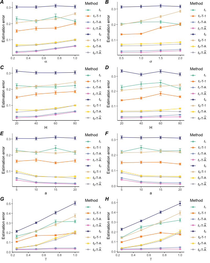
Figure 3: Estimation results in Scenario 2. From left to right: Configurations 1 and 2. From top to bottom: performances with varying discrepancy levels ($\alpha$ and $\sigma$), difference vector changing frequencies ($H$), cardinalities of the informative set ($a$) and change magnitudes ($\gamma$), respectively.

References

- Arnold and Tibshirani (2014) Taylor B. Arnold and Ryan J. Tibshirani. genlasso: Path algorithm for generalized lasso problems, 2014. URL http://CRAN.R-project.org/package=genlasso. R package version 1.3.
- Bastani (2021) Hamsa Bastani. Predicting with proxies: Transfer learning in high dimension. Management Science, 67(5):2964–2984, 2021.
- Cai and Pu (2022) T Tony Cai and Hongming Pu. Transfer learning for nonparametric regression: Non-asymptotic minimax analysis and adaptive procedure. arXiv preprint arXiv:0000.0000, 2022.
- Cai and Wei (2019) T. Tony Cai and Hongji Wei. Transfer learning for nonparametric classification: Minimax rate and adaptive classifier, 2019.
- Cai et al. (2023) T Tony Cai, Dongwoo Kim, and Hongming Pu. Transfer learning for functional mean estimation: Phase transition and adaptive algorithms. http://www-stat.wharton.upenn.edu/ tcai/paper/html/Transfer-Learning-Mean-Function.html, 2023.
- Daumé III (2009) Hal Daumé III. Frustratingly easy domain adaptation. In Proceedings of the 45th annual meeting of the association of computational linguistics, pages 256–263, 2009.
- Fan and Lv (2008) Jianqing Fan and Jinchi Lv. Sure independence screening for ultrahigh dimensional feature space. Journal of the Royal Statistical Society Series B: Statistical Methodology, 70(5):849–911, 2008.
- Fan and Guan (2018) Zhou Fan and Leying Guan. Approximate -penalized estimation of piecewise-constant signals on graphs. The Annals of Statistics, 46(6B):3217–3245, 2018.
- Friedrich et al. (2008) Felix Friedrich, Angela Kempe, Volkmar Liebscher, and Gerhard Winkler. Complexity penalized m-estimation: fast computation. Journal of Computational and Graphical Statistics, 17(1):201–224, 2008.
- Guntuboyina et al. (2020) Adityanand Guntuboyina, Donovan Lieu, Sabyasachi Chatterjee, and Bodhisattva Sen. Adaptive risk bounds in univariate total variation denoising and trend filtering. The Annals of Statistics, 48(1):205–229, 2020.
- Independent Statistics and Analysis (2023) Independent Statistics and Analysis. U.s. energy information administration, 2023. URL https://www.eia.gov/electricity/.
- Johnson (2013) Nicholas Johnson. A dynamic programming algorithm for the fused lasso and -segmentation. Journal of Computational and Graphical Statistics, 22(2):246–260, 2013.
- Li et al. (2022) Sai Li, T Tony Cai, and Hongzhe Li. Transfer learning for high-dimensional linear regression: Prediction, estimation and minimax optimality. Journal of the Royal Statistical Society Series B: Statistical Methodology, 84(1):149–173, 2022.
- Li et al. (2023) Sai Li, Linjun Zhang, T Tony Cai, and Hongzhe Li. Estimation and inference for high-dimensional generalized linear models with knowledge transfer. Journal of the American Statistical Association, pages 1–12, 2023.
- Lin et al. (2017) Kevin Lin, James L Sharpnack, Alessandro Rinaldo, and Ryan J Tibshirani. A sharp error analysis for the fused lasso, with application to approximate changepoint screening. In Advances in Neural Information Processing Systems, pages 6884–6893, 2017.