High-order geometric integrators for the local cubic variational Gaussian wavepacket dynamics

Abstract

Gaussian wavepacket dynamics has proven to be a useful semiclassical approximation for quantum simulations of high-dimensional systems with low anharmonicity. Compared to Heller’s original local harmonic method, the variational Gaussian wavepacket dynamics is more accurate, but much more difficult to apply in practice because it requires evaluating the expectation values of the potential energy, gradient, and Hessian. If the variational approach is applied to the local cubic approximation of the potential, these expectation values can be evaluated analytically, but still require the costly third derivative of the potential. To reduce the cost of the resulting local cubic variational Gaussian wavepacket dynamics, we describe efficient high-order geometric integrators, which are symplectic, time-reversible, and norm-conserving. For small time steps, they also conserve the effective energy. We demonstrate the efficiency and geometric properties of these integrators numerically on a multi-dimensional, nonseparable coupled Morse potential.

I Introduction

Gaussian wavepackets provide an explicit link between the classical and quantum dynamics. [1] Because they are localized in space, Gaussian wavepackets only require information about the potential in a specific region of configuration space, and thus can substantially reduce the cost of molecular quantum dynamics simulations. Inspired by the pioneering work of Heller, [2, 3, 4] a number of multi-trajectory Gaussian-based methods, such as the Herman-Kluk initial value representation, [5, 6, 7] multiple spawning, [8, 9, 10] variational multiconfigurational Gaussians,[11] coupled coherent states,[12] multiconfigurational Ehrenfest method,[13] or Gaussian dephasing representation, [14] were proposed to approximate the solution of the time-dependent Schrödinger equation (TDSE). Because the local nature of Gaussian wavepackets allows the potential to be calculated “on the fly,” many of these methods were combined with an on-the-fly ab initio evaluation of the electronic structure. [15, 16, 17, 18, 19, 20, 21, 22, 23]

The multi-trajectory methods typically require a large number of trajectories to converge, and therefore, single-trajectory Gaussian-based methods have recently re-emerged as a practical alternative. Although they cannot capture wavepacket splitting, the single-trajectory methods, such as divide-and-conquer semiclassical dynamics,[24, 25] ab initio thawed Gaussian approximation, [26, 27, 28, 29] and its more efficient single Hessian version, [30, 31, 32, 33] have proven sufficiently accurate in weakly anharmonic systems of rather large dimension. Moreover, thanks to their efficiency, these methods can afford more accurate electronic structure theory.

Among the single-trajectory Gaussian-based methods, the most accurate one is the variational Gaussian wavepacket dynamics (variational GWD), [34, 35, 36, 37, 38, 39] obtained by applying the time-dependent variational principle [40, 41, 36] to a thawed Gaussian ansatz (“thawed” means that the Gaussian has a flexible width, which we will always assume). Not only is the variational GWD symplectic and time-reversible, but it also conserves the norm and energy of the wavepacket.[42, 39] The method is, however, hard to apply to “real-world” problems because it requires expectation values of the potential and its derivatives, which typically cannot be evaluated analytically and are also very difficult to compute numerically. One way to surmount this obstacle is to approximate the potential $V$ by its Taylor expansion $V_{\text{appr }}$around the center of the Gaussian since the expectation values of $V_{\text{appr}}$ and its derivatives are readily evaluated analytically. Replacing the expectation values of the original potential, gradient, and Hessian with the corresponding values of $V_{\text{appr}}$ in the equations of motion of the variational GWD yields a method, which is easily applied to any potential $V$, including that obtained from an on-the-fly ab initio evaluation of the electronic structure. Using the local harmonic approximation of the potential ($V_{\text{appr}}=V_{\text{LHA}}$) reduces the variational method to Heller’s celebrated thawed Gaussian approximation, [2, 43, 44] which is, however, neither symplectic nor energy-conserving and cannot capture tunneling. [39]

In contrast, the local cubic variational GWD, obtained by applying the local cubic approximation to the potential ($V_{\text{appr}}=V_{\text{LCA}}$), is symplectic, [45, 46] conserves the effective energy, [47, 38] and may capture tunneling because the guiding trajectory is nonclassical. [48] This remarkable method was originally studied by Pattanayak and Schieve [47, 49] under the name “extended semiclassical wavepacket dynamics” and later, in depth, by Ohsawa and co-workers, [48, 45, 46] who called it “symplectic semiclassical wavepacket dynamics.” The local cubic variational GWD, which is also norm-conserving and time-reversible, preserves all the geometric properties of the fully variational GWD, except that it conserves the effective rather than the exact energy. The improvements over Heller’s local harmonic GWD, however, come at a high cost of evaluating the symmetric rank-three tensor of third derivatives of $V$ along the trajectory.

To make this appealing method more practical, in this paper, our goal is reducing the computational cost of the local cubic variational GWD without sacrificing its geometric properties. In the case of local harmonic GWD, it was shown that using a single, i.e., constant Hessian along the whole trajectory speeds up the method and, in addition, results in the conservation of both symplectic structure and effective energy. [30, 38] Applying a similar trick to the local cubic variational GWD, namely, using a single third derivative, however, breaks the symplecticity and effective energy conservation. Therefore, to improve the efficiency of the local cubic method, we implement and analyze high-order geometric integrators, which are analogous to the integrators we recently implemented for the fully variational GWD [39] and which are a special case of general integrators for GWD described in Ref. 38.

The rest of this paper is organized as follows: In Sec. II, we review the variational GWD and derive equations of motion for the GWD when the potential is approximated by either the local harmonic or local cubic expansion. After discussing the remarkable geometric properties of the local cubic variational GWD in Sec. III, in Sec. IV we describe efficient high-order geometric integrators that preserve most of these properties exactly. Section V provides numerical examples that demonstrate the improved accuracy and geometric properties of the local cubic variational GWD compared to the original local harmonic method and that confirm the fast convergence, increased efficiency, and geometric properties of the high-order integrators in various many-dimensional anharmonic systems. Section VI concludes the paper.

II Local cubic variational Gaussian wavepacket dynamics

II.1 Gaussian wavepacket dynamics

The GWD approximates the solution of the TDSE

$$i\hbar\,d|\psi_{t}\rangle/dt=\hat{H}|\psi_{t}\rangle$$ (1)

with a complex Gaussian ansatz,

$$\psi_{t}(q)=\text{exp}\bigg{[}\frac{i}{\hbar}\bigg{(}\frac{1}{2}\,x^{T}\cdot A_{t}\cdot x+p_{t}^{T}\cdot x+\gamma_{t}\bigg{)}\bigg{]},$$ (2)

where $x:=q-q_{t}$ is the difference position vector, $q_{t}$ and $p_{t}$ are the $D$-dimensional real vectors denoting the position and momentum of the Gaussian’s center, $A_{t}$ is a $D\times D$ complex symmetric width matrix with a positive-definite imaginary part, and $\gamma_{t}$ is a complex number whose real part represents a phase and whose imaginary part ensures normalization of $\psi_{t}$. In Eq. (1), $\hat{H}\equiv H(\hat{q},\hat{p})$ is a Hamiltonian operator separable into a sum

$$\hat{H}=T(\hat{p})+V(\hat{q})$$ (3)

of the kinetic energy operator $T(\hat{p})=\hat{p}^{T}\cdot m^{-1}\cdot\hat{p}/2$, depending only on momentum $p$, and the potential energy operator $V(\hat{q})$, depending only on position $q$. $m$ is the real-symmetric mass matrix. It can be shown [38] that the GWD for Eq. (1) can be viewed as the exact solution of the nonlinear TDSE [50, 51]

$$i\hbar\,d|\psi_{t}\rangle/dt=\hat{H}_{\text{eff}}(\psi_{t})|\psi_{t}\rangle$$ (4)

with an effective, state-dependent Hamiltonian operator

$$\hat{H}_{\text{eff}}(\psi_{t})=T(\hat{p})+V_{\text{eff}}(\hat{q};\psi_{t}),$$ (5)

where $V_{\text{eff}}(\hat{q};\psi_{t})$ is an effective quadratic potential [38, 39]

$$V_{\text{eff}}(q;\psi_{t})=V_{0}+V_{1}^{T}\cdot x+x^{T}\cdot V_{2}\cdot x/2.$$ (6)

The coefficients $V_{0}$, $V_{1}$, and $V_{2}$ may depend on the state $\psi_{t}$ and are different for each of the GWD methods. In a general GWD, the parameters of the Gaussian wavepacket (2) satisfy the system

$$\dot{q}_{t} =m^{-1}\cdot p_{t},$$ (7)

$$\dot{p}_{t} =-V_{1},$$ (8)

$$\dot{A}_{t} =-A_{t}\cdot m^{-1}\cdot A_{t}-V_{2},$$ (9)

$$\dot{\gamma}_{t} =T(p_{t})-V_{0}+(i\hbar/2)\,\text{Tr}(m^{-1}\cdot A_{t})$$ (10)

of first-order ordinary differential equations. [38]

II.2 Fully variational GWD

The variational GWD employs the time-dependent variational principle [40, 41, 36] to optimally approximate the solution of the TDSE (1) with the Gaussian ansatz (2). In the variational GWD, the effective potential (6) has the coefficients [38, 39]

$$V_{0}=\langle\hat{V}\rangle-\text{Tr}\big{(}{\langle\hat{V}^{\prime\prime}\rangle}\cdot\Sigma_{t}\big{)}/2,\quad V_{1}=\langle\hat{V}^{\prime}\rangle,\quad V_{2}=\langle\hat{V}^{\prime\prime}\rangle.$$ (11)

Above and throughout this paper, we use a shorthand notation $\langle\hat{O}\rangle:=\langle\psi_{t}|\hat{O}|\psi_{t}\rangle$ for the expectation value of the operator $\hat{O}$ in the Gaussian wavepacket $\psi_{t}$. In Eq. (11), $\hat{V}^{\prime}:=V^{\prime}(q)|_{q=\hat{q}}$ and $\hat{V}^{\prime\prime}:=V^{\prime\prime}(q)|_{q=\hat{q}}$ are the gradient and Hessian of the potential energy operator, and

$$\Sigma_{t}:=\langle\hat{x}\otimes\hat{x}^{T}\rangle=(\hbar/2)\,(\text{Im}A_{t})^{-1}$$ (12)

is the position covariance. [52] Therefore, the equations of motion for the variational method include expectation values of the potential and its derivatives, which generally cannot be evaluated analytically. Since the expectation value of a polynomial operator in a Gaussian can be obtained exactly, in the following sections, we approximate the potential by its second- and third-order Taylor expansions about the Gaussian’s center and obtain the modified equations of motion for the variational GWD.

II.3 Local harmonic (variational) GWD = Heller’s GWD

Replacing the exact potential $V(q)$ in Eq. (11) with its local harmonic approximation (LHA)

$$V_{\text{LHA}}(q,\psi_{t})=V(q_{t})+V^{\prime}(q_{t})^{T}\cdot x+x^{T}\cdot V^{\prime\prime}(q_{t})\cdot x/2$$ (13)

gives[38]

$$V_{0}=V(q_{t}),\quad V_{1}=V^{\prime}(q_{t}),\quad V_{2}=V^{\prime\prime}(q_{t}).$$ (14)

Equations (7)-(10) with coefficients (14) are exactly the equations of motion of Heller’s original thawed Gaussian approximation.[2, 26] This local harmonic GWD is very efficient and easy to implement, but preserves neither the effective nor the exact energy. [38] Moreover, since the Gaussian’s center $(q_{t},p_{t})$ evolves according to classical Hamilton’s equations of motion [Eqs. (7) and (8) with coefficients (14)], the local harmonic GWD cannot capture quantum tunneling.

II.4 Local cubic variational GWD

To improve upon the local harmonic GWD, one needs to replace the potential with a more accurate approximation. Let us, therefore, apply the variational GWD to the local cubic approximation (LCA)

$$V_{\text{LCA}}(q,\psi_{t}) =V(q_{t})+V^{\prime}(q_{t})^{T}\cdot x+x^{T}\cdot V^{\prime\prime}(q_{t})\cdot x/2$$

$$\quad+V^{\prime\prime\prime}(q_{t})_{ijk}\,x_{i}x_{j}x_{k}/3!$$ (15)

of the potential $V$, where $V^{\prime\prime\prime}$ is the rank-3 tensor of the third derivatives of the potential $V$. The gradient and Hessian of the $V_{\text{LCA}}$ are

$$V_{\text{LCA}}^{\prime}(q,\psi_{t})_{i} =V^{\prime}(q_{t})_{i}+V^{\prime\prime}(q_{t})_{ij}\,x_{j}$$

$$\quad+V^{\prime\prime\prime}(q_{t})_{ijk}\,x_{j}x_{k}/2,$$ (16)

$$V_{\text{LCA}}^{\prime\prime}(q,\psi_{t})_{ij} =V^{\prime\prime}(q_{t})_{ij}+V^{\prime\prime\prime}(q_{t})_{ijk}\,x_{k}.$$ (17)

By substituting expectation values

$$\langle\hat{V}_{\text{LCA}}\rangle =V(q_{t})+\text{Tr}\big{[}V^{\prime\prime}(q_{t})\cdot\Sigma_{t}\big{]}/2,$$

$$\langle\hat{V}_{\text{LCA}}^{\prime}\rangle_{i} =V^{\prime}(q_{t})_{i}+V^{\prime\prime\prime}(q_{t})_{ijk}\,\Sigma_{t,jk}/2,$$ (18)

$$\langle\hat{V}_{\text{LCA}}^{\prime\prime}\rangle =V^{\prime\prime}(q_{t})$$

into Eq. (11), we get the effective potential coefficients

$$V_{0} =V(q_{t}),$$

$$V_{1,i} =V^{\prime}(q_{t})_{i}+V^{\prime\prime\prime}(q_{t})_{ijk}\,\Sigma_{t,jk}/2,$$ (19)

$$V_{2} =V^{\prime\prime}(q_{t}).$$

The equations of motion of the resulting “local cubic variational GWD”,

$$\dot{q}_{t} =m^{-1}\cdot p_{t},$$ (20)

$$\big{(}\dot{p}_{t}\big{)}_{i} =-V^{\prime}(q_{t})_{i}-V^{\prime\prime\prime}(q_{t})_{ijk}\,\Sigma_{t,jk}/2,$$ (21)

$$\dot{A}_{t} =-A_{t}\cdot m^{-1}\cdot A_{t}-V^{\prime\prime}(q_{t}),$$ (22)

$$\dot{\gamma}_{t} =T(p_{t})-V(q_{t})+(i\hbar/2)\,\text{Tr}(m^{-1}\cdot A_{t}),$$ (23)

are identical to those of the local harmonic GWD except for a non-classical force term $-V^{\prime\prime\prime}(q_{t})_{ijk}\,\Sigma_{t,jk}/2$ in the equation for $\dot{p}_{t}$. The local cubic variational GWD is equivalent to Ohsawa and Leok’s “symplectic semiclassical wavepacket dynamics” [48, 45, 46] and Pattanayak and Schieve’s “extended semiclassical dynamics”. [49] Remarkably, in contrast to the local harmonic GWD, the local cubic method is symplectic, conserves the effective energy, [38] and may capture tunneling because the Gaussian follows a nonclassical trajectory. [48]

Let us mention that the utility of the local cubic expansion of the PES is not restricted to single-trajectory methods—this expansion was also used for evaluating the matrix elements of the potential needed in the calculation of the absorption spectrum of formaldehyde with the on-the-fly variational multiconfigurational Gaussian method; there, too, the local cubic expansion was found to yield more accurate results than the local harmonic approximation. [53]

III Geometric properties of the local cubic variational GWD

In the local cubic variational GWD, the Gaussian wavepacket evolves according to a nonlinear TDSE (4) in a state-dependent effective quadratic potential (6) with coefficients (19). As any other exact solution of the more general nonlinear TDSE (4), the local cubic variational GWD is time-reversible and norm-conserving, but does not conserve the inner product and distance. [50, 38] Unlike some other GWD methods, the local cubic variational method is symplectic [48] and, although it is not energy-conserving, it does conserve the effective energy exactly. [38] Let us discuss the last three properties in more detail.

III.1 Energy

The energy of a Gaussian wavepacket can be computed as the expectation value

$$E:=\langle\hat{H}\rangle=\langle\hat{T}\rangle+\langle\hat{V}\rangle$$ (24)

of the separable Hamiltonian (3). In Eq. (24),

$$\langle\hat{T}\rangle=T(p_{t})+\text{Tr}\big{[}m^{-1}\cdot\text{Cov}(\hat{p})\big{]}/2$$ (25)

is the kinetic energy, [38] $\langle\hat{V}\rangle$ is the potential energy, and

$$\text{Cov}(\hat{p}) :=\langle(\hat{p}-p_{t})\otimes(\hat{p}-p_{t})^{T}\rangle$$

$$\,\,=(\hbar/2)\,A_{t}\cdot(\text{Im}\,A_{t})^{-1}\cdot A_{t}^{{\dagger}}$$ (26)

is the momentum covariance. [38] In general GWD, the energy depends on time as [see Eq. (21) in Ref. 38]:

$$\dot{E}=\text{Re}\,\big{\langle}\hat{p}^{T}\cdot m^{-1}\cdot(\hat{V}^{\prime}-\hat{V}_{\text{eff}}^{\prime})\big{\rangle}.$$ (27)

For the local cubic method with coefficients (19), we have

$$V_{\text{eff}}^{\prime}(q,\psi_{t})_{i} =V^{\prime}(q_{t})_{i}+V^{\prime\prime\prime}(q_{t})_{ijk}\,\Sigma_{t,jk}/2+V^{\prime\prime}(q_{t})_{ij}\,x_{j}$$

$$\neq V^{\prime}(q)_{i}.$$ (28)

Therefore, the local cubic variational GWD does not conserve energy,[38] even though the fully variational GWD is energy-conserving. [39, 37]

III.2 Effective energy

The effective energy of a Gaussian wavepacket driven by the effective Hamiltonian (5) can be evaluated as

$$E_{\text{eff}}:=\langle\hat{H}_{\text{eff}}\rangle=\langle\hat{T}\rangle+\langle\hat{V}_{\text{eff}}\rangle,$$ (29)

where $\langle\hat{T}\rangle$ is given in Eq. (25) and $\langle\hat{V}_{\text{eff}}\rangle$ for the local cubic variational GWD is obtained from Eqs. (6) and (19),

$$\langle\hat{V}_{\text{eff}}\rangle=V(q_{t})+\text{Tr}\big{[}V^{\prime\prime}(q_{t})\cdot\Sigma_{t}\big{]}/2.$$ (30)

The time dependence of the effective energy (29) is [see Eq. (22) in Ref. 38]:

$$\dot{E}_{\text{eff}}=\dot{V}_{0}-V_{1}^{T}\cdot\dot{q}_{t}+\text{Tr}\big{(}\dot{V}_{2}\cdot\Sigma_{t}\big{)}/2.$$ (31)

Inserting “local cubic” coefficients (19) into Eq. (31) gives

$$\dot{E}_{\text{eff}} =V^{\prime}(q_{t})^{T}\cdot\dot{q}_{t}-V^{\prime}(q_{t})^{T}\cdot\dot{q}_{t}-V^{\prime\prime\prime}(q_{t})_{ijk}\,\Sigma_{t,jk}\dot{q}_{t,i}/2$$

$$\quad+V^{\prime\prime\prime}(q_{t})_{ijk}\,\Sigma_{t,jk}\dot{q}_{t,i}/2=0,$$ (32)

and thus, unlike the local harmonic GWD, the local cubic variational method does conserve the effective energy.

III.3 Symplecticity

Faou and Lubich demonstrated the non-canonical symplectic structure of the variational GWD. [42] Ohsawa and Leok showed that the local cubic variational GWD is a non-canonical Hamiltonian system whose equations of motion are precisely Eqs. (20)-(23). [48] Omitting the phase factor $\exp(i\,\text{Re}\,\gamma_{t}/\hbar)$ in (2) corresponds to an equivalent representation of the Gaussian wavepacket (without a phase) in a projective Hilbert space with a phase symmetry. [46, 45] Furthermore, the imaginary part of the parameter $\gamma_{t}$ ensures normalization of the Gaussian wavepacket and can be expressed in terms of the imaginary part of the width $A_{t}$ [Eq. (52)]. Without the parameter $\gamma$, the symplectic manifold parametrized by the set $(q,p,\text{Re}\,A,\text{Im}\,A)$ has the reduced symplectic form [46, 45]

$$\omega(z)=dq_{j}\wedge dp_{j}+(\hbar/4)\,d\,\big{[}(\text{Im}\,A)^{-1}\big{]}_{kl}\wedge d\,\text{Re}\,A_{kl},$$ (33)

where the first term is the standard classical symplectic structure and the second term could be called the “quantum” component of the symplectic structure.

IV Geometric integrators for the local cubic variational GWD

Geometric integrators for the nonlinear TDSE (4) with a general effective potential (6) were presented in Ref. 38. The only and rather weak assumption necessary for obtaining explicit integrators was that the coefficients $V_{0}$, $V_{1}$, and $V_{2}$ of the effective potential (6) depended on the wavepacket $\psi_{t}$ only through $q_{t}$ and $\text{Im}\,A_{t}$ and were independent of $p_{t}$, $\text{Re}\,A_{t}$, and $\gamma_{t}$. In Ref. 39, we investigated these geometric integrators for the variational GWD and showed that the high-order integrators could be more efficient and more accurate at the same time. Here, we describe, implement, and analyze such geometric integrators for the local cubic variational GWD.

IV.1 Second-order geometric integrator

The simplest, first-order algorithm is based on the decomposition of the separable, effective Hamiltonian (5) into the kinetic and potential terms. This makes it possible to solve the equations of motion (20)-(23) analytically. During the kinetic propagation $[\hat{H}_{\text{eff}}=T(\hat{p})$, i.e., $V=0]$, Eqs. (20)-(23) have the analytical solution

$$q_{t} =q_{0}+t\,m^{-1}\cdot p_{0},$$ (34)

$$p_{t} =p_{0},$$ (35)

$$A_{t} =(A_{0}^{-1}+t\,m^{-1})^{-1},$$ (36)

$$\gamma_{t} =\gamma_{0}+t\,T(p_{0})$$

$$\quad+(i\hbar/2)\,\text{ln}\,[\,\text{det}\,(I_{D}+t\,m^{-1}\cdot A_{0})],$$ (37)

where $I_{D}$ is the $D\times D$ identity matrix, and during the potential propagation $[\hat{H}_{\text{eff}}=V_{\text{eff}}(\hat{q})$, i.e., $m^{-1}=0]$, Eqs. (20)-(23) have the analytical solution

$$q_{t} =q_{0},$$ (38)

$$p_{t,i} =p_{0,i}-t\,V^{\prime}(q_{0})_{i}-t\,V^{\prime\prime\prime}(q_{0})_{ijk}\,\Sigma_{0,jk}/2,$$ (39)

$$A_{t} =A_{0}-t\,V^{\prime\prime}(q_{0}),$$ (40)

$$\gamma_{t} =\gamma_{0}-t\,V(q_{0}).$$ (41)

By sequentially performing potential propagation for time $\Delta t/2$, kinetic propagation for time $\Delta t$, and potential propagation for time $\Delta t/2$, one obtains the second-order “potential-kinetic-potential”(VTV) algorithm. Swapping the kinetic and potential propagation steps gives the second-order “kinetic-potential-kinetic”(TVT) algorithm. Each of the two numerical algorithms gives the state $\psi_{t+\Delta t}$ at time $t+\Delta t$ from the state $\psi_{t}$ at time $t$:

$$|\psi_{t+\Delta t}\rangle=\hat{U}_{2}(t+\Delta t,t;\psi)|\psi_{t}\rangle,$$ (42)

where $\hat{U}_{2}$ is the approximate second-order evolution operator associated with the VTV or TVT algorithm. Note that these algorithms are analogues of Faou and Lubich’s second-order geometric integrator for the variational GWD. [42, 54]

IV.2 High-order geometric integrators

An appropriate composition of the second order (VTV or TVT) algorithm (42) yields integrators of higher order of accuracy. [54, 55, 56, 57, 58, 59, 60, 61, 62] More precisely, any symmetric evolution operator $\hat{U}_{p}$ of even order $p$ yields an evolution operator $\hat{U}_{p+2}$ of order $p+2$ if it is symmetrically composed as [54]

$$\hat{U}_{p+2}(t+\Delta t,t;\psi) :=\hat{U}_{p}(t+\xi_{M}\Delta t,t+\xi_{M-1}\Delta t;\psi)$$

$$\qquad\qquad\cdots\hat{U}_{p}(t+\xi_{1}\Delta t,t;\psi),$$ (43)

where $M$ is the total number of composition steps and $\xi_{n}:=\sum_{j=1}^{n}\gamma_{j}$ denotes the sum of the first $n$ real composition coefficients $\gamma_{j}$. The choice of the composition coefficients must satisfy the relations $\sum_{j=1}^{M}\gamma_{j}=1$ (consistency), $\gamma_{M+1-j}=\gamma_{j}$ (symmetry), and $\sum_{j=1}^{M}\gamma_{j}^{p+1}=0$ (order increase guarantee). [54] The simplest symmetric composition methods are the recursive triple-jump [56] with $M=3$ and Suzuki’s fractal [57] with $M=5$. Both methods can produce high-order integrators. Because the number of composition steps and thus the computational cost grows exponentially with the order of convergence, here we only use the more efficient, non-recursive composition schemes that are, in a certain sense, optimal. Kahan and Li [63] obtained optimal composition methods for the sixth and eighth orders by minimizing $\max_{j}|\gamma_{j}|$, and Sofroniou and Spaletta [60] found the tenth order optimal composition scheme by minimizing $\sum_{j=1}^{M}|\gamma_{j}|$. Suzuki’s fractal gives the optimal fourth-order scheme. [61] For more details on the general as well as optimal composition methods, see Ref. 61.

IV.3 Geometric properties of the geometric integrators

In the splitting algorithm described by Eqs. (34)-(41), each potential or kinetic step of the local cubic variational GWD is solved exactly. Therefore, before the composition, each kinetic or potential step has all the geometric properties of the local cubic variational method. All integrators, obtained by symmetric compositions of the exact solutions (34)-(41) of the kinetic and potential propagation steps, are time-reversible and conserve the norm and symplectic structure (see Appendix B for an explicit proof of symplecticity). However, due to the splitting, they conserve the effective energy only approximately, with an error $O(\Delta t^{M})$ where the power $M$ is equal to or greater than the order of the algorithm. For general proofs of these statements see Refs. 55, 54, 62, 61, 50.

V Numerical examples

In the following, we investigate the local cubic variational GWD and the proposed high-order integrators in several anharmonic model systems. Our calculations show (i) the superior accuracy of the local cubic variational method over the local harmonic GWD, (ii) the conservation of the effective energy by the local cubic variational method, (iii) the preservation of the geometric properties of the local cubic variational method by the geometric integrators, and (iv) the efficiency of the high-order integrators. All values are presented in natural units (n.u.): $\hbar=m=1$. We do not show the results of the VTV algorithm and its compositions since they are almost identical to the corresponding results of the TVT algorithm.

To analyze the error due to the local cubic approximation of the potential, we compare the local cubic variational with the fully variational results. For numerical experiments, we have therefore chosen the coupled Morse potential, for which the expectation values of the potential energy, gradient, and Hessian, needed in the fully variational GWD, can be computed analytically.

The nonseparable, $D$-dimensional “coupled Morse potential” [39]

$$V(q)=V_{\text{eq}}+\sum_{j=1}^{D}V_{j}(q_{j})+V_{\text{cpl}}(q)$$ (44)

consists of $D$ independent one-dimensional Morse potentials $V_{j}(q_{j})$, which are coupled by a “multidimensional Morse coupling” $V_{\text{cpl}}(q)$, and $V_{\text{eq}}$ is the potential at the equilibrium bond distance $q_{\text{eq}}$. Each one-dimensional Morse potential

$$V_{j}(q_{j}):=d_{e}^{\prime}\,\big{[}1-y_{j}(a_{j}^{\prime},q_{j})\big{]}^{2}$$ (45)

depends on the dissociation energy $d_{e}^{\prime}$ and one-dimensional Morse variable [64]

$$y_{j}(a_{j}^{\prime},q_{j}):=\exp\big{[}-a_{j}^{\prime}\,(q_{j}-q_{\text{eq},j})\big{]},$$ (46)

which, in turn, is a function of the decay parameter $a_{j}^{\prime}$ and $q_{j}$. The $D$-dimensional coupling term

$$V_{\text{cpl}}(q):=d_{e}\,\big{[}1-y(a,q)\big{]}^{2}$$ (47)

depends on the dissociation energy $d_{e}$ and $D$-dimensional Morse variable

$$y(a,q):=\exp\big{[}-a^{T}\cdot(q-q_{\text{eq}})\big{]},$$ (48)

which, in turn, is a function of the decay vector $a$ and $q$. The decay parameter $a_{j}^{\prime}$, dissociation energy $d_{e}^{\prime}$, and dimensionless anharmonicity $\chi_{j}^{\prime}$ are connected by the relation $a_{j}^{\prime}=\chi_{j}^{\prime}\,\sqrt{8\,d_{e}^{\prime}}$. [30] Likewise, the decay vector $a$, dissociation energy $d_{e}$, and dimensionless anharmonicity vector $\chi$ are related via $a=\chi\,\sqrt{8\,d_{e}}$. The derivatives and expectation values of the coupled Morse potential (44) are given in Ref. 39.

V.1 One-dimensional Morse potential

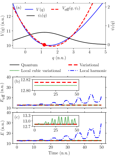
Figure 1: Dynamics of a wavepacket $\psi_{t}$ in a one-dimensional Morse potential $V$. Panel (a) shows the effective potential $V_{\textrm{eff}}$ of the local cubic variational GWD. Panels (b) and (c) compare the effective $(E_{\textrm{eff}})$ and exact $(E)$ energies of the wavepacket propagated with different methods. For clarity, the insets of panels (b) and (c) do not show the local harmonic results.

Figures 1-4 analyze the dynamics of a Gaussian wavepacket in a standard one-dimensional Morse potential, which is also a special case of the coupled Morse potential (44) with zero coupling term ($d_{e}=0$) in Eq. (47). The potential parameters are $q_{\text{eq}}=1.5$, $V_{\text{eq}}=10$, $d_{e}^{\prime}=22.5$, and anharmonicity $\chi^{\prime}=0.01$. The initial wavepacket was a real Gaussian with $q_{0}=-0.5$, $p_{0}=0$, and $A_{0}=i\omega_{0}$, which is also the ground vibrational state of a harmonic potential with frequency $\omega_{0}=1$. This wavepacket was propagated for $5000$ steps of $\Delta t=0.01$ with different GWD methods using the second-order geometric integrator from Sec. IV or with the quantum dynamics using the analogous second-order split-operator algorithm. The position grid for the quantum dynamics consisted of $513$ equidistant ($\Delta q=30/512$) points between $-5$ and $25$.

Panel (a) of Fig. 1 shows a snapshot at time $t=8.8$ of the wavepacket propagated with the local cubic variational GWD. Note that the associated effective potential $V_{\text{eff}}$ is not tangent to the exact potential $V$, and thus differs from the local harmonic approximation. Panels (b) and (c) compare the effective and exact energies of the wavepacket propagated with different methods. The effective and exact energies of the variational GWD are equal and conserved. Panel (b) shows that, unlike the local harmonic method, the local cubic approach conserves its effective energy. Panel (c) indicates that the energy of the local cubic method is not conserved. However, its deviation from the exact value is significantly smaller than that of the local harmonic one.

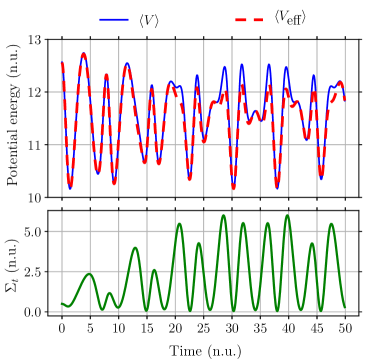
Figure 2: Top panel compares the exact and effective potential energies of a Gaussian wavepacket propagated in a one-dimensional Morse potential with the local cubic variational GWD. These two energies are almost equal whenever the position covariance, shown in the bottom panel, is small.

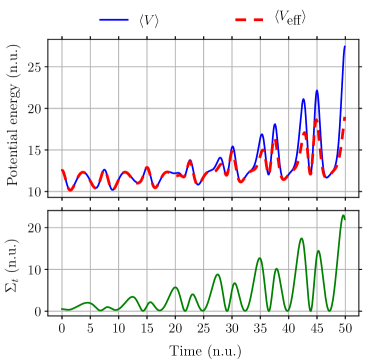
Figure 3: Top panel compares the exact and effective potential energies of a Gaussian wavepacket propagated in a one-dimensional Morse potential with the local harmonic GWD. These two energies are almost identical whenever the position covariance, shown in the bottom panel, is small.

The expectation values of the exact and effective potential energies are compared in Fig. 2 for the local cubic variational GWD and in Fig. 3 for the local harmonic GWD. Both figures confirm that the difference between the exact and effective potential energies increases with time. However, this increase is more pronounced in the local harmonic method. The lower panels of Figs. 2 and 3 show the position covariance (12), which is basically the squared width of a one-dimensional Gaussian wavepacket. In both figures, the exact and effective potential energies are almost identical at local minima of the position covariance, since at these times the Gaussian wavepacket becomes infinitesimally narrow, and the potential is thus approximated over a smaller region of space. In contrast, the exact and effective potential energies differ the most at local maxima of the position covariance.

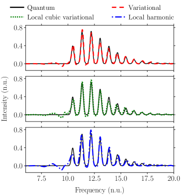
Figure 4: Absorption spectrum of a one-dimensional Morse potential with anharmonicity $\chi=0.01$. The spectra obtained with the (a) variational, (b) local cubic variational, and (c) local harmonic GWD are compared to the exact quantum spectrum.

We also calculated the absorption spectrum, corresponding to the electronic transition from a harmonic PES to the just described Morse PES, as the Fourier transform [65, 66, 67, 1, 68]

$$\sigma(\omega)=\text{Re}\int_{0}^{\infty}C(t)\,e^{i(\omega+E_{1,g}/\hbar)t}\,dt$$ (49)

of the wavepacket autocorrelation function

$$C(t)=\langle\psi_{0}|\psi_{t}\rangle,$$ (50)

where $E_{1,g}$ is the vibrational zero point energy of state $\psi_{0}$ in the harmonic PES before photon absorption. The overlap (50) of Gaussian wavepackets $\psi_{0}$ and $\psi_{t}$ is given by Eq. (29) in Ref. 28 or by Eq. (B4) in Ref. 39.

Figure 4 compares spectra computed with different methods. To obtain smooth spectra, the simulation time in Fig. 4 was ten times longer than the simulation time in Fig. 1. A Gaussian damping function with a half-width at half-maximum of $10$ was applied to each autocorrelation function before computing the spectrum by Fourier transform. All three semiclassical methods perform well in the calculation of spectra, but the nonlinear character of their effective Hamiltonian (5) leads to small, yet visible unphysical negative intensities. As expected, the fully variational spectrum is slightly more accurate than the local cubic variational one, and its negative features are smaller. Similarly, the local cubic variational spectrum is more accurate than the local harmonic one, especially in the low-frequency region and in the high-frequency tail.

V.2 Two-dimensional coupled Morse potential

Figures 5 and 6 analyze the dynamics of a wavepacket in a two-dimensional coupled Morse potential (44) with energy $V_{\text{eq}}=10$ at the equilibrium position $q_{\text{eq}}=(1,1)$. The potential is composed of two one-dimensional Morse potentials with the same dissociation energy $d_{e}^{\prime}=11.25$ and different anharmonicities $\chi_{1}^{\prime}=0.02$ and $\chi_{2}^{\prime}=0.017$. The parameters of the coupling term are $d_{e}=5.75$ and $\chi=(0.014,0.017)$. The initial wavepacket was a real two-dimensional Gaussian (2) with $q_{0}=(-0.75,1.75)$, $p_{0}=(0,0)$, and a diagonal width matrix $A_{0}$ with non-zero elements $A_{0,11}=A_{0,22}=i$. This wavepacket was propagated for $20000$ steps of $\Delta t=0.001$ with different methods using the second-order geometric or split-operator integrator. The position grid for the exact quantum dynamics consisted of $257$ equidistant $(\Delta q=20/256)$ points between $-5$ and $15$ in both directions.

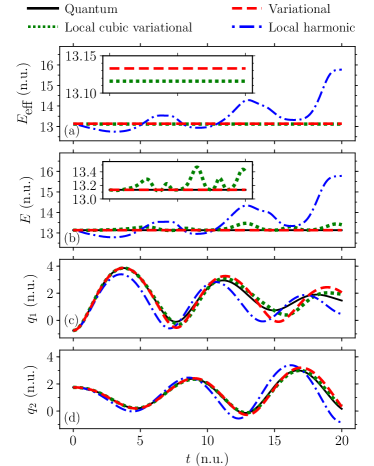
Figure 5: Dynamics of a wavepacket propagated in a two-dimensional coupled Morse potential with different methods. Effective energy [panel (a)], energy [panel (b)], and position of the Gaussian’s center along two different coordinates [panels (c) and (d)] are shown. For clarity, the insets of panels (a) and (b) do not show the local harmonic results.

Panels (a) and (b) of Fig. 5 confirm our observations for the one-dimensional Morse potential in Fig. 1: (i) the effective and exact energies of the fully variational method are conserved and equal to each other and to the quantum energy, (ii) the local cubic variational GWD conserves the effective energy, but not the exact energy, and (iii) the local harmonic GWD conserves neither the effective nor the exact energy. Panels (c) and (d) show the expectation values of the position of the wavepacket. For very short times, all approximations give accurate quantum results, but their accuracy decreases with time. However, the variational and local cubic variational methods remain accurate longer than the local harmonic GWD. The spectra of this two-dimensional coupled Morse potential, calculated with different methods, are available in the supplementary material.

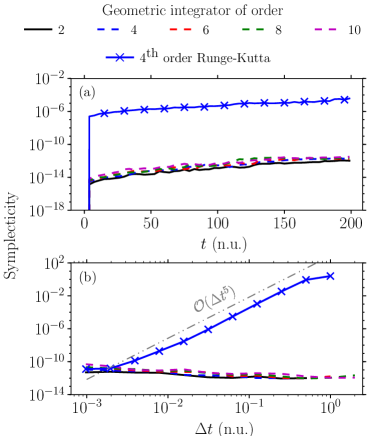
Figure 6: Conservation of the symplectic structure of the Gaussian wavepackets by the geometric integrators and its nonconservation by the fourth-order Runge-Kutta method. The system is the same two-dimensional coupled Morse potential as in Fig. 5. The symplecticity (51) is shown (a) as a function of time $t$ for a fixed and fairly large time step $\Delta t=2^{-4}\,\textrm{n.u.}$ and (b) as a function of time step $\Delta t$ at the final time $t_{f}=200\,\textrm{n.u.}$

In Fig. 6, we analyze the symplecticity of the geometric integrators for the local cubic variational GWD. We verified the symplecticity numerically by measuring the distance

$$d \big{(}\Phi_{t}^{\prime}(z_{0})^{T}\cdot\omega(z_{t})\cdot\Phi_{t}^{\prime}(z_{0}),\omega(z_{0})\big{)}$$

$$\equiv\lVert\Phi_{t}^{\prime}(z_{0})^{T}\cdot\omega(z_{t})\cdot\Phi_{t}^{\prime}(z_{0})-\omega(z_{0})\rVert$$ (51)

between the “initial” and “final” symplectic structure matrices $\omega(z_{0})$ and $\omega(z_{t})$. Here, the vector $z$ contains elements of the Gaussian’s parameters propagated by a numerical integrator with flow $\Phi_{t}(z)$ and Jacobian $\Phi_{t}^{\prime}(z)$, and $\omega(z)$ is a skew-symmetric matrix representing the non-canonical symplectic two-form of Gaussian wavepackets. Hagedorn proposed a different but equivalent parametrization of the Gaussian wavepacket, [69] in which the equations of motion of the GWD become simpler (see Appendix A). We, therefore, evaluated the Jacobian and symplecticity in Hagedorn’s parametrization; see Appendix B for more details.

Figure 6 shows the symplecticity (51) of the Gaussian wavepacket propagated with the local cubic variational GWD in the two-dimensional coupled Morse potential analyzed in Fig. 5. Although the simulation time in Fig.  6 is ten times longer than the simulation time in Fig. 5, all geometric integrators conserve the non-canonical symplectic structure exactly, regardless of the size of the time step. In contrast, the figure clearly shows that the fourth-order Runge-Kutta method [55] does not conserve the symplectic structure of the local cubic variational GWD.

V.3 Twenty-dimensional coupled Morse potential

Figures 7-11 analyze the dynamics of a Gaussian wavepacket in a twenty-dimensional coupled Morse potential (44) composed of twenty one-dimensional Morse potentials (45) with the same dissociation energy $d_{e}^{\prime}=0.1$ and with anharmonicity parameters $\chi_{j}^{\prime}\,\,(j=1,\dots,20)$ uniformly varying in the range between $0.001$ and $0.005$ $(\Delta\chi^{\prime}=0.004/19)$. Parameters of the coupling term (47) were $d_{e}=0.075$ and $\chi_{j}=(3/4)\,\chi_{j}^{\prime}$, and the energy at the equilibrium position $q_{\text{eq},j}=10\,\,(j=1,\dots,20)$ was $V_{\text{eq}}=0$. The twenty-dimensional real initial Gaussian wavepacket had zero position, zero momentum, and a diagonal width matrix with non-zero elements $A_{jj}=4\,d_{e}\chi_{j}\,i$.

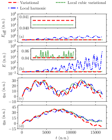
Figure 7: Dynamics of a Gaussian wavepacket propagated in a twenty-dimensional coupled Morse potential with various GWD methods. Effective energy [panel (a)], energy [panel (b)], and position of the Gaussian’s center along two different coordinates [panels (c) and (d)] are shown. For clarity, the insets of panels (a) and (b) do not show the local harmonic results.

In Fig. 7, this wavepacket was propagated for $2^{17}=131072$ steps of $\Delta t=0.125$ with various GWD methods using the second-order geometric integrator. Unlike Fig. 5, Fig. 7 lacks the exact quantum benchmark because the system is not solvable by the grid-based methods due to its high dimensionality. Even using the multi-configurational time-dependent Hartree method, [70, 71] exact quantum calculation for this high-dimensional system would be very difficult. Panels (a) and (b) of Fig. 7 show the exact and effective energies of the wavepacket propagated with different semiclassical methods. The effective and exact energies of the fully variational method are equal and conserved. Both the effective and exact energies of the wavepacket propagated with the local cubic variational or local harmonic GWD differ from the corresponding energies obtained by the variational GWD. However, the difference is much greater for the local harmonic GWD, especially at longer times. Furthermore, unlike the local harmonic GWD, the local cubic variational GWD conserves its effective energy. Panels (c) and (d) display the position of the Gaussian’s center. For very short times, all semiclassical methods overlap almost perfectly. However, the local cubic variational results remain close to the fully variational results for longer times.

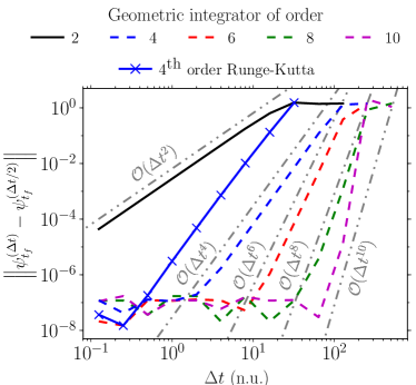
Figure 8: Convergence of various integrators for the local cubic variational GWD, measured by the convergence error at the final time $t_{f}=2^{16}\,\textrm{n.u.}=65536\,\textrm{n.u.}$ as a function of the time step $\Delta t$. The convergence error is defined as the distance $d(\psi^{(\Delta t)}_{t},\psi^{(\Delta t/2)}_{t})\equiv\lVert\psi^{(\Delta t)}_{t}-\psi^{(\Delta t/2)}_{t}\rVert$, where $\psi^{(\Delta t)}_{t}$ denotes the state at time $t$ obtained after propagation with time step $\Delta t$.

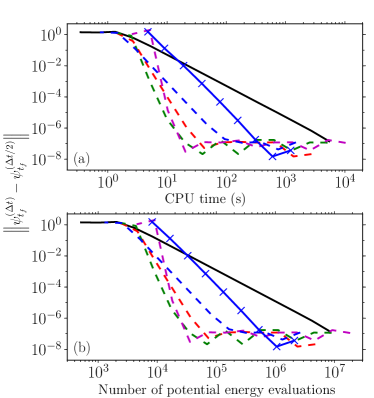
Figure 9: Efficiency of various integrators for the local cubic variational GWD. Efficiency is measured by plotting the convergence error, defined in the caption of Fig. 8, as a function of (a) the computational cost (CPU time) or (b) the number of potential energy evaluations. Line labels are the same as those in Fig. 8.

To analyze the convergence and geometric properties of the integrators, we repeated the local cubic variational simulation with several high-order geometric integrators and with the fourth-order Runge-Kutta method.

Convergence rates of various methods are compared in Fig. 8. For all methods, the obtained orders of convergence agree with the predicted ones, indicated by the gray straight lines. The plateau indicates the machine precision error. Since the high-order methods require a large number of composition substeps to be carried out at each time step $\Delta t$, a higher order of convergence does not guarantee higher efficiency. Figure 9 measures the efficiency directly by plotting the convergence error as a function of either the CPU time or the number of potential energy evaluations. The similarity between panels (a) and (b) confirms that the cost of initialization and finalization is negligible to the cost of potential propagation; this will be even more the case in expensive on-the-fly ab initio applications. In addition, Fig. 9 shows that high-order geometric integrators are more efficient than both the second-order geometric integrator and the fourth-order Runge-Kutta method. For example, below a rather large error of $10^{-1}$, the eighth-order integrator is more efficient than the sixth-, fourth-, and second-order integrators, and for a moderate error of $10^{-4}$, the fourth-order geometric integrator is almost $10$ times faster than the second-order geometric algorithm and almost $3.5$ faster than the fourth-order Runge-Kutta method. As a result, the use of high-order geometric integrators can simultaneously increase both accuracy and efficiency.

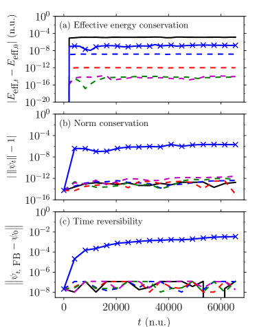
Figure 10: Geometric properties of various integrators for the local cubic variational GWD as a function of time $t$ for a relatively large time step $\Delta t=8\,\textrm{n.u.}$ (a) Effective energy, (b) norm, and (c) time reversibility [Eq. (53)] are shown. Line labels are the same as those in Fig. 8.

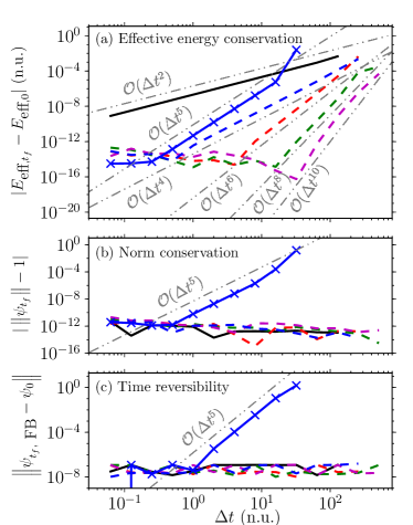
Figure 11: Geometric properties of various integrators for the local cubic variational GWD as a function of the time step $\Delta t$ measured at the final time $t_{f}=2^{16}\,\textrm{n.u.}=65536\,\textrm{n.u.}$ (a) Effective energy, (b) norm, and (c) time reversibility [Eq. (53)] are shown. Line labels are the same as those in Fig. 8.

Figure 10 shows how the effective energy, norm, and time reversibility depend on time, whereas Fig. 11 analyzes how these geometric properties depend on the time step. Panels (a) of both figures analyze the conservation of the effective energy measured by the difference $|E_{\text{eff},t}-E_{\text{eff},0}|$. Although the local cubic variational GWD conserves the effective energy, the splitting nature of the geometric integrators reduces this exact conservation. [54, 62] This is because the alternation between kinetic [$\hat{H}_{\mathrm{eff}}=T(\hat{p})$] and potential [$\hat{H}_{\mathrm{eff}}=V_{\mathrm{eff}}(\hat{q})$] propagations makes the effective Hamiltonian time-dependent. The geometric integrators and the fourth-order Runge-Kutta method conserve the effective energy only approximately, with the order in $\Delta t$ equal to or greater than their order of convergence. Conservation of the norm is measured by the deviation $|\lVert\psi_{t}\rVert-1|$, where

$$\lVert\psi_{t}\rVert=\text{exp}(-\text{Im}\,\gamma_{t}/\hbar)\,\big{[}\text{det}(\pi\hbar/\text{Im}\,A_{t})\big{]}^{1/4}$$ (52)

is the norm of the Gaussian wavepacket (2). Unlike the effective energy, which is conserved only approximately, panels (b) of Figs. 10 and 11 confirm the exact norm conservation by the geometric integrators. The fourth-order Runge-Kutta method, on the other hand, fails to conserve the norm unless it is fully converged, which requires using a very small time step. In panels (c) of Figs. 10 and 11, the time reversibility is checked by plotting the distance

$$d\big{(}\psi_{t,\text{FB}},\psi_{0}\big{)}\equiv\lVert\psi_{t,\text{FB}}-\psi_{0}\rVert$$ (53)

between the initial state $\psi_{0}$ and the “forward-backward” propagated state $\psi_{t,\text{FB}}$ (i.e., the state propagated first forward in time for time $t$ and then backward in time for time $t$). Unlike the fourth-order Runge-Kutta method, the geometric integrators are exactly time-reversible. Note that the convergence of norm, energy, and reversibility by the fourth-order Runge-Kutta method appears to be $\mathcal{O}(\Delta t^{5})$, i.e., faster than $\mathcal{O}(\Delta t^{4})$.

We do not repeat the analysis of symplecticity, which was analyzed for the two-dimensional coupled Morse potential in Fig. 6, because its evaluation for the twenty-dimensional system is unnecessarily expensive. Finally, as any exact solution of a genuinely nonlinear TDSE, the local cubic variational GWD conserves neither the inner product nor the distance between two states (see Fig. S2 in the supplementary material).

VI Conclusion

We have shown that applying the local cubic approximation to the potential in the variational GWD improves the accuracy over Heller’s original GWD, which is based only on the local harmonic approximation. In contrast to the original GWD, the local cubic variational method is symplectic and conserves the effective energy. Most importantly, the local cubic method is also a practical implementation of the variational method for future on-the-fly ab initio applications, since it avoids the difficult evaluation of $\langle\hat{V}\rangle$, $\langle\hat{V}^{\prime}\rangle$, and $\langle\hat{V}^{\prime\prime}\rangle$. Although more accurate than the local harmonic GWD, the local cubic variational method significantly increases the computational cost because it requires the third derivative of the potential along the trajectory. To partially ameliorate this issue, we accelerated the method by designing and implementing high-order geometric integrators. We showed that these high-order integrators not only increased the efficiency and accuracy over the second-order algorithm, but also preserved most geometric properties of the local cubic variational GWD. Although the local cubic variational method is only a crude approximation of the exact solution of the TDSE in anharmonic systems, our well-converged results obtained with the high-order integrators ensure that the numerical errors are negligible.

In conclusion, the local cubic variational GWD is promising for future on-the-fly ab initio applications to medium-sized molecules. We expect it to account more accurately for anharmonic effects, especially in ultrafast spectroscopy, where only short-time dynamics is required. Its potential to approximately include tunneling also deserves further attention.

Supplementary material

See the supplementary material for the absorption spectra of the two-dimensional coupled Morse potential from Sec. V.2 and for the numerical demonstration of the nonconservation of the inner product and distance by the local cubic variational GWD.

Data availability

The data that support the findings of this study are available within the article and its supplementary material.

Appendix A Gaussian wavepacket dynamics in Hagedorn’s parametrization

In Hagedorn’s parametrization, [69] the Gaussian wavepacket (2) is written as

$$\psi_{t}(q)=(\pi\hbar)^{-D/4}(\text{det}\,Q_{t})^{-1/2}$$

$$\quad\times\text{exp}\bigg{[}\frac{i}{\hbar}\bigg{(}\frac{1}{2}\,x^{T}\cdot P_{t}\cdot Q^{-1}_{t}\cdot x+p_{t}^{T}\cdot x+S_{t}\bigg{)}\bigg{]},$$ (54)

where the new parameters $Q_{t}$ and $P_{t}$ are two $D\times D$ complex matrices, related to the width of the Gaussian by $A_{t}=P_{t}\cdot Q^{-1}_{t}$ and satisfying the relations [69, 36]

$$Q^{T}_{t}\cdot P_{t}-P^{T}_{t}\cdot Q_{t}=0,$$ (55)

$$Q^{\dagger}_{t}\cdot P_{t}-P^{\dagger}_{t}\cdot Q_{t}=2iI_{D},$$ (56)

and $S_{t}$ is a real scalar that generalizes the classical action.

Equations of motion for $\dot{q}_{t}$ and $\dot{p}_{t}$ [Eqs. (7) and (8)] remain unchanged, whereas the equations for $\dot{A}_{t}$ and $\dot{\gamma}_{t}$ [Eqs. (9) and (10)] are replaced by

$$\dot{Q}_{t} =m^{-1}\cdot P_{t},$$ (57)

$$\dot{P}_{t} =-V_{2}\cdot Q_{t},$$ (58)

$$\dot{S}_{t} =T(p_{t})-V_{0}.$$ (59)

A.1 Geometric integrators in Hagedorn’s parametrization

In Hagedorn’s parametrization, the kinetic propagation flow $\Phi_{\text{T},t}$ is [38]

$$q_{t} =q_{0}+t\,m^{-1}\cdot p_{0},$$ (60)

$$p_{t} =p_{0},$$ (61)

$$Q_{t} =Q_{0}+t\,m^{-1}\cdot P_{0},$$ (62)

$$P_{t} =P_{0},$$ (63)

$$S_{t} =S_{0}+t\,T(p_{0}),$$ (64)

whereas the potential propagation flow $\Phi_{\text{V},t}$ is [38]

$$q_{t} =q_{0},$$ (65)

$$p_{t} =p_{0}-t\,V_{1}(q_{0},Q_{0}),$$ (66)

$$Q_{t} =Q_{0},$$ (67)

$$P_{t} =P_{0}-t\,V_{2}(q_{0},Q_{0})\cdot Q_{0},$$ (68)

$$S_{t} =S_{0}-t\,V_{0}(q_{0},Q_{0}).$$ (69)

Appendix B Symplecticity of the geometric integrators

To verify the symplecticity of a numerical integrator designed for the GWD, one should show that the Jacobian $\Phi_{t}^{\prime}(z_{0})$ of the integrator with the flow $z_{t}=\Phi_{t}(z_{0})$ satisfies the condition [54]

$$\Phi_{t}^{\prime}(z_{0})^{T}\cdot\omega(z_{t})\cdot\Phi_{t}^{\prime}(z_{0})=\omega(z_{0}),$$ (70)

where $z_{t}$ is a vector containing the Gaussian’s parameters and $\omega(z_{t})$ is the symplectic structure of the Gaussian wavepackets. [Note that matrix $\omega$ in Eq. (70) is the inverse of matrix $B$ appearing in Eq. (4.2) of Chapter VII of Ref. 54).]

In Hagedorn’s parametrization, the reduced symplectic form (33) becomes the standard symplectic form [46]

$$\omega(z) =dq_{j}\wedge dp_{j}+(\hbar/2)\,dQ_{kl}^{(1)}\wedge dP_{kl}^{(1)}$$

$$\quad+(\hbar/2)\,dQ_{kl}^{(2)}\wedge dP_{kl}^{(2)}$$ (71)

with

$$z_{t}:=\bigg{(}q_{t}^{T},p_{t}^{T},\widetilde{Q_{t}^{(1)}}^{T},\widetilde{P_{t}^{(1)}}^{T},\widetilde{Q_{t}^{(2)}}^{T},\widetilde{P_{t}^{(2)}}^{T}\bigg{)}^{T}\in\mathbb{R}^{2D+4D^{2}},$$

where $Q_{t}^{(1)}$ and $Q_{t}^{(2)}$ are real and imaginary parts of matrix $Q_{t}=Q_{t}^{(1)}+iQ_{t}^{(2)}$, and $P_{t}^{(1)}$ and $P_{t}^{(2)}$ are real and imaginary parts of matrix $P_{t}=P_{t}^{(1)}+iP_{t}^{(2)}$. Moreover, $\widetilde{\Lambda}$, which is used for $\Lambda=Q_{t}^{(1)},P_{t}^{(1)},Q_{t}^{(2)}$, and $P_{t}^{(2)}$, is a $D^{2}$-dimensional vector containing elements of the $D\times D$ matrix $\Lambda$ in a column-by-column manner, i.e., $\widetilde{\Lambda}_{j+D(k-1)}=\Lambda_{jk}$. Matrix representation of (71) is the constant $(2D+4D^{2})$-dimensional block-diagonal matrix

$$\omega(z_{t})=\begin{pmatrix}J_{2D}&0&0\\ 0&\frac{\hbar}{2}J_{2D^{2}}&0\\ 0&0&\frac{\hbar}{2}J_{2D^{2}}\end{pmatrix}.$$ (72)

In Eq. (72), $J_{2D^{2}}=J_{2D}\otimes I_{D}$ and $J_{2D}=J_{2}\otimes I_{D}$, where

$$J_{2}=\begin{pmatrix}0&1\\ -1&0\end{pmatrix}$$ (73)

is the canonical $2\times 2$ symplectic matrix.

The flow of a geometric integrator of any order is composed of a sequence of kinetic and potential flows. Its Jacobian is therefore equal to the matrix product of the Jacobians of the elementary flows. To demonstrate the symplecticity of geometric integrators, we first analyze the symplecticity of the kinetic and potential flows.

B.1 Symplecticity of the kinetic flow

The kinetic flow $\Phi_{\text{T},t}(z_{0})$ given by Eqs. (60)-(63) does not depend on the coefficients $V_{0}$, $V_{1}$, and $V_{2}$, and thus is identical for all GWD methods. The Jacobian of this flow is the block-diagonal matrix [39]

$$\Phi_{\text{T},t}^{\prime}(z_{0})=\begin{pmatrix}M_{2D}&0&0\\ 0&M_{2D^{2}}&0\\ 0&0&M_{2D^{2}}\end{pmatrix},$$ (74)

where

$$M_{2D}=\begin{pmatrix}I_{D}&t\,m^{-1}\\ 0&I_{D}\end{pmatrix}$$ (75)

is the stability matrix and $M_{2D^{2}}=M_{2D}\otimes I_{D}$. The kinetic flow with Jacobian (74) is symplectic, i.e., $\Phi_{\text{T},t}^{\prime}(z_{0})^{T}\cdot\omega(z_{t})\cdot\Phi_{\text{T},t}^{\prime}(z_{0})=\omega(z_{0}),$ because

$$M_{2D}^{T}\cdot J_{2D}\cdot M_{2D}=\begin{pmatrix}I_{D}&0\\ t\,m^{-1}&I_{D}\end{pmatrix}\begin{pmatrix}0&I_{D}\\ -I_{D}&-t\,m^{-1}\end{pmatrix}=J_{2D}$$ (76)

and, due to the relation between matrix and tensor multiplications,

$$M_{2D^{2}}^{T} \cdot J_{2D^{2}}\cdot M_{2D^{2}}$$

$$=\big{(}M_{2D}^{T}\otimes I_{D}\big{)}\cdot\big{(}J_{2D}\otimes I_{D}\big{)}\cdot\big{(}M_{2D}\otimes I_{D}\big{)}$$

$$=\big{(}M_{2D}^{T}\cdot J_{2D}\cdot M_{2D}\big{)}\otimes I_{D}=J_{2D^{2}}.$$ (77)

B.2 Symplecticity of the potential flow

Inserting the coefficients $V_{0}$, $V_{1}$, and $V_{2}$ of the fully variational GWD [Eq. (11)], the local harmonic GWD [Eq. (14)], or the local cubic variational GWD [Eq. (19)] into Eqs. (65)-(68) gives the potential flow $\Phi_{\text{V},t}(z_{0})$ for the corresponding methods. The Jacobian of this potential flow is the $(2D+4D^{2})$-dimensional matrix

$$\Phi_{\text{V},t}^{\prime}(z_{0})=I_{2D+4D^{2}}-t\begin{pmatrix}0&0&0&0&0&0\\ a&0&b^{(1)}&0&b^{(2)}&0\\ 0&0&0&0&0&0\\ c^{(1)}&0&d^{(11)}&0&d^{(12)}&0\\ 0&0&0&0&0&0\\ c^{(2)}&0&d^{(21)}&0&d^{(22)}&0\end{pmatrix},$$ (78)

where

$$a_{j,k} =\partial V_{1}(q_{0},Q_{0})_{j}/\partial q_{0,k},$$ (79)

$$b_{j,D(k-1)+l}^{(r)} =\partial V_{1}(q_{0},Q_{0})_{j}/\partial Q_{0,kl}^{(r)},$$ (80)

$$c_{D(j-1)+k,l}^{(r)} =\partial\big{[}V_{2}(q_{0},Q_{0})_{jm}\,Q_{0,mk}^{(r)}\big{]}/\partial q_{0,l},$$ (81)

$$d_{D(j-1)+k,\,D(l-1)+m}^{(rs)} =\partial\big{[}V_{2}(q_{0},Q_{0})_{jn}\,Q_{0,nk}^{(r)}\big{]}/\partial Q_{0,lm}^{(s)}$$

$$=\big{[}\partial V_{2}(q_{0},Q_{0})_{jn}/\partial Q_{0,lm}^{(s)}\big{]}\,Q_{0,nk}^{(r)}$$

$$\quad+V_{2}(q_{0},Q_{0})_{jn}\,\delta_{nl}\,\delta_{km}\,\delta_{rs}$$ (82)

are, respectively, components of a $D\times D$ matrix $a$, a $D\times D^{2}$ matrix $b^{(r)}$, a $D^{2}\times D$ matrix $c^{(r)}$, and a $D^{2}\times D^{2}$ matrix $d^{(rs)}$ for all $r,s\in\{1,2\}$. Satisfaction of the relation $\Phi_{\text{V},t}^{\prime}(z_{0})^{T}\cdot\omega(z_{t})\cdot\Phi_{\text{V},t}^{\prime}(z_{0})=\omega(z_{0})$ requires that

$$a^{T}=a,\qquad\big{(}b^{(r)}\big{)}^{T}=(\hbar/2)\,c^{(r)},\qquad\big{(}d^{(rs)}\big{)}^{T}=d^{(sr)}.$$ (83)

Since the coefficients (11) of the fully variational GWD depend on $\langle\hat{V}\rangle$, $\langle\hat{V}^{\prime}\rangle$, and $\langle\hat{V}^{\prime}\rangle$, which, in turn, depend only on $q_{0}$ and $Q_{0}$, in Eqs. (79)-(82) we only need expressions for the derivatives of $\langle\hat{V}^{(n)}\rangle$ with respect to $q_{0}$ and $Q_{0}$. The former is

$$\partial\langle\hat{V}^{(n)}\rangle/\partial q_{0}=\langle\hat{V}^{(n+1)}\rangle,$$ (84)

while the latter can be found in Eq. (B30) in Ref. 39. Using these two relations, we conclude that

$$a_{j,k} =\langle\hat{V}^{\prime\prime}\rangle_{jk},$$ (85)

$$b_{j,D(k-1)+l}^{(r)} =(\hbar/2)\,\langle\hat{V}^{\prime\prime\prime}\rangle_{jkm}\,Q_{0,ml}^{(r)},$$ (86)

$$c_{D(j-1)+k,l}^{(r)} =\langle\hat{V}^{\prime\prime\prime}\rangle_{jml}\,Q_{0,mk}^{(r)},$$ (87)

$$d_{D(j-1)+k,\,D(l-1)+m}^{(rs)} =(\hbar/2)\,\langle\hat{V}^{(4)}\rangle_{jnlp}\,Q_{0,nk}^{(r)}\,Q_{0,pm}^{(s)}$$

$$\quad+\langle\hat{V}^{\prime\prime}\rangle_{jn}\,\delta_{nl}\,\delta_{km}\,\delta_{rs}.$$ (88)

Because $\langle\hat{V}^{\prime\prime}\rangle$, $\langle\hat{V}^{\prime\prime\prime}\rangle$, and $\langle\hat{V}^{(4)}\rangle$ are totally symmetric, Eqs. (85)-(88) for $a$, $b^{(r)}$, $c^{(r)}$, and $d^{(rs)}$ imply that conditions (83) hold for the Jacobian (78), and thus the potential flow of the variational GWD is symplectic.

Finally, inserting coefficients (14) of the local harmonic GWD into Eqs. (79)-(82) yields

$$a_{j,k} =V^{\prime\prime}(q_{0})_{jk},$$ (89)

$$b_{j,D(k-1)+l}^{(r)} =0,$$ (90)

$$c_{D(j-1)+k,l}^{(r)} =V^{\prime\prime\prime}(q_{0})_{jml}\,Q_{0,mk}^{(r)},$$ (91)

$$d_{D(j-1)+k,\,D(l-1)+m}^{(rs)} =V^{\prime\prime}(q_{0})_{jn}\,\delta_{nl}\,\delta_{km}\,\delta_{rs}.$$ (92)

Equations (90) and (91) imply that the second condition in (83) is not fulfilled, and therefore the local harmonic GWD is not symplectic.

Inserting coefficients (19) of the local cubic variational GWD into Eqs. (79)-(82) yields

$$a_{j,k} =V^{\prime\prime}(q_{0})_{jk}$$

$$\quad+V^{(4)}(q_{0})_{jklm}\,\Sigma_{0,lm}/2,$$ (93)

$$b_{j,D(k-1)+l}^{(r)} =(\hbar/2)\,V^{\prime\prime\prime}(q_{0})_{jkm}\,Q_{0,ml}^{(r)},$$ (94)

$$c_{D(j-1)+k,l}^{(r)} =V^{\prime\prime\prime}(q_{0})_{jml}\,Q_{0,mk}^{(r)},$$ (95)

$$d_{D(j-1)+k,\,D(l-1)+m}^{(rs)} =V^{\prime\prime}(q_{0})_{jn}\,\delta_{nl}\,\delta_{km}\,\delta_{rs},$$ (96)

where we used the position covariance in Hagedorn’s parametrization, [52] $\Sigma_{t}:=(\hbar/2)\,Q_{t}\cdot Q_{t}^{\dagger}$, to derive (94). The conditions (83) are satisfied for (78) because $V^{\prime\prime}$, $V^{\prime\prime\prime}$, and the fourth derivative $V^{(4)}$ of the potential, in Eqs.(93)-(96), are totally symmetric. Hence, the potential flow of the local cubic variational GWD is symplectic.

B.3 Symplecticity of the composed geometric integrators

If both kinetic and potential flows are symplectic, then any composition of them is symplectic. This proves the conservation of the symplectic structure (71) by the geometric integrators developed for the fully variational and local cubic variational GWD, since the composed flow $\Phi_{t}(z_{0})$ of a geometric integrator consists of many steps, each of which consists of several potential and kinetic substeps. In Ref. 39 and in Sec. V.2, we verified symplecticity of these integrators numerically by measuring the accuracy with which Eq. (70) is satisfied if $\Phi_{t}(z_{0})$ denotes the composed flow consisting many steps, each of which, in turn, is composed by several kinetic and potential substeps. For that, Jacobian $\Phi_{t}^{\prime}(z_{0})$ of the composed flow appearing in Eq. (70) was obtained by matrix multiplication of the Jacobians of all kinetic and potential steps.

References

- Tannor [2007] D. J. Tannor, Introduction to Quantum Mechanics: A Time-Dependent Perspective (University Science Books, Sausalito, 2007).
- Heller [1975] E. J. Heller, J. Chem. Phys. 62, 1544 (1975).
- Heller [1976a] E. J. Heller, J. Chem. Phys. 65, 4979 (1976a).
- Heller [1981a] E. J. Heller, J. Chem. Phys. 75, 2923 (1981a).
- Herman and Kluk [1984] M. F. Herman and E. Kluk, Chem. Phys. 91, 27 (1984).
- Walton and Manolopoulos [1995] A. R. Walton and D. E. Manolopoulos, Chem. Phys. Lett. 244, 448 (1995).
- Miller [2001] W. H. Miller, J. Phys. Chem. A 105, 2942 (2001).
- Martínez, Ben-Nun, and Levine [1996] T. J. Martínez, M. Ben-Nun, and R. D. Levine, J. Phys. C 100, 7884 (1996).
- Ben-Nun, Quenneville, and Martínez [2000] M. Ben-Nun, J. Quenneville, and T. J. Martínez, J. Phys. Chem. A 104, 5161 (2000).
- Curchod and Martínez [2018] B. F. E. Curchod and T. J. Martínez, Chem. Rev. 118, 3305 (2018).
- Worth and Burghardt [2003] G. A. Worth and I. Burghardt, Chem. Phys. Lett. 368, 502 (2003).
- Shalashilin and Child [2000] D. V. Shalashilin and M. S. Child, J. Chem. Phys. 113, 10028 (2000).
- Shalashilin [2009] D. V. Shalashilin, J. Chem. Phys. 130, 244101 (2009).
- Šulc et al. [2013] M. Šulc, H. Hernández, T. J. Martínez, and J. Vaníček, J. Chem. Phys. 139, 034112 (2013).
- Tatchen and Pollak [2009] J. Tatchen and E. Pollak, J. Chem. Phys. 130, 041103 (2009).
- Ceotto et al. [2009] M. Ceotto, S. Atahan, G. F. Tantardini, and A. Aspuru-Guzik, J. Chem. Phys. 130, 234113 (2009).
- Wong et al. [2011] S. Y. Y. Wong, D. M. Benoit, M. Lewerenz, A. Brown, and P.-N. Roy, J. Chem. Phys. 134, 094110 (2011).
- Botti, Ceotto, and Conte [2021] G. Botti, M. Ceotto, and R. Conte, J. Chem. Phys. 155, 234102 (2021).
- Levine et al. [2008] B. G. Levine, J. D. Coe, A. M. Virshup, and T. J. Martínez, Chem. Phys. 347, 3 (2008).
- Levine and Martínez [2009] B. G. Levine and T. J. Martínez, J. Phys. Chem. A 113, 12815 (2009).
- Bramley, Symonds, and Shalashilin [2019] O. Bramley, C. Symonds, and D. V. Shalashilin, J. Chem. Phys. 151, 064103 (2019).
- Worth, Robb, and Burghardt [2004] G. A. Worth, M. A. Robb, and I. Burghardt, Faraday Discuss. 127, 307 (2004).
- Saita and Shalashilin [2012] K. Saita and D. V. Shalashilin, J. Chem. Phys. 137, 22A506 (2012).
- Ceotto, Di Liberto, and Conte [2017] M. Ceotto, G. Di Liberto, and R. Conte, Phys. Rev. Lett. 119, 010401 (2017).
- Gabas, Di Liberto, and Ceotto [2019] F. Gabas, G. Di Liberto, and M. Ceotto, J. Chem. Phys. 150, 224107 (2019).
- Wehrle, Šulc, and Vaníček [2014] M. Wehrle, M. Šulc, and J. Vaníček, J. Chem. Phys. 140, 244114 (2014).
- Wehrle, Oberli, and Vaníček [2015] M. Wehrle, S. Oberli, and J. Vaníček, J. Phys. Chem. A 119, 5685 (2015).
- Begušić and Vaníček [2020] T. Begušić and J. Vaníček, J. Chem. Phys. 153, 184110 (2020).
- Kletnieks, Alonso, and Vanicek [2023] E. Kletnieks, Y. C. Alonso, and J. J. L. Vanicek, J. Phys. Chem. A 127, 8117 (2023).
- Begušić, Cordova, and Vaníček [2019] T. Begušić, M. Cordova, and J. Vaníček, J. Chem. Phys. 150, 154117 (2019).
- Prlj et al. [2020] A. Prlj, T. Begušić, Z. T. Zhang, G. C. Fish, M. Wehrle, T. Zimmermann, S. Choi, J. Roulet, J.-E. Moser, and J. Vaníček, J. Chem. Theory Comput. 16, 2617 (2020).
- Begušić, Tapavicza, and Vaníček [2022] T. Begušić, E. Tapavicza, and J. J. L. Vaníček, J. Chem. Theory Comput. 18, 3065 (2022).
- Golubev, Begušić, and Vaníček [2020] N. V. Golubev, T. Begušić, and J. Vaníček, Phys. Rev. Lett. 125, 083001 (2020).
- Heller [1976b] E. J. Heller, J. Chem. Phys. 64, 63 (1976b).
- Coalson and Karplus [1990] R. D. Coalson and M. Karplus, J. Chem. Phys. 93, 3919 (1990).
- Lubich [2008] C. Lubich, From Quantum to Classical Molecular Dynamics: Reduced Models and Numerical Analysis, 12th ed. (European Mathematical Society, Zürich, 2008).
- Lasser and Lubich [2020] C. Lasser and C. Lubich, Acta Numerica 29, 229 (2020).
- Vaníček [2023] J. J. L. Vaníček, J. Chem. Phys. 159, 014114 (2023).
- Moghaddasi Fereidani and Vaníček [2023] R. Moghaddasi Fereidani and J. J. L. Vaníček, J. Chem. Phys. 159, 094114 (2023).
- Dirac [1930] P. A. M. Dirac, Math. Proc. Camb. Phil. Soc. 26, 376 (1930).
- Frenkel [1934] J. Frenkel, Wave mechanics (Clarendon Press, Oxford, 1934).
- Faou and Lubich [2006] E. Faou and C. Lubich, Comput. Visual. Sci. 9, 45 (2006).
- Lee and Heller [1982] S.-Y. Lee and E. J. Heller, J. Chem. Phys. 76, 3035 (1982).
- Heller [2018] E. J. Heller, The semiclassical way to dynamics and spectroscopy (Princeton University Press, Princeton, NJ, 2018).
- Ohsawa [2015a] T. Ohsawa, J. Math. Phys. 56, 032103 (2015a).
- Ohsawa [2015b] T. Ohsawa, Lett. Math. Phys. 105, 1301 (2015b).
- Pattanayak and Schieve [1994a] A. K. Pattanayak and W. C. Schieve, Phys. Rev. Lett. 72, 2855 (1994a).
- Ohsawa and Leok [2013] T. Ohsawa and M. Leok, J. Phys. A 46, 405201 (2013).
- Pattanayak and Schieve [1994b] A. K. Pattanayak and W. C. Schieve, Phys. Rev. E 50, 3601 (1994b).
- Roulet and Vaníček [2021a] J. Roulet and J. Vaníček, J. Chem. Phys. 154, 154106 (2021a).
- Roulet and Vaníček [2021b] J. Roulet and J. Vaníček, J. Chem. Phys. 155, 204109 (2021b).
- Vaníček and Begušić [2021] J. Vaníček and T. Begušić, in Molecular Spectroscopy and Quantum Dynamics, edited by R. Marquardt and M. Quack (Elsevier, 2021) pp. 199–229.
- Bonfanti et al. [2018] M. Bonfanti, J. Petersen, P. Eisenbrandt, I. Burghardt, and E. Pollak, J. Chem. Theory Comput. 14, 5310 (2018).
- Hairer, Lubich, and Wanner [2006] E. Hairer, C. Lubich, and G. Wanner, Geometric Numerical Integration: Structure-Preserving Algorithms for Ordinary Differential Equations (Springer Berlin Heidelberg New York, 2006).
- Leimkuhler and Reich [2004] B. Leimkuhler and S. Reich, Simulating Hamiltonian Dynamics (Cambridge University Press, 2004).
- Yoshida [1990] H. Yoshida, Phys. Lett. A 150, 262 (1990).
- Suzuki [1990] M. Suzuki, Phys. Lett. A 146, 319 (1990).
- McLachlan [1995] R. I. McLachlan, SIAM J. Sci. Comp. 16, 151 (1995).
- Wehrle, Šulc, and Vaníček [2011] M. Wehrle, M. Šulc, and J. Vaníček, Chimia 65, 334 (2011).
- Sofroniou and Spaletta [2005] M. Sofroniou and G. Spaletta, Optim. Method Softw. 20, 597 (2005).
- Choi and Vaníček [2019] S. Choi and J. Vaníček, J. Chem. Phys. 150, 204112 (2019).
- Roulet, Choi, and Vaníček [2019] J. Roulet, S. Choi, and J. Vaníček, J. Chem. Phys. 150, 204113 (2019).
- Kahan and Li [1997] W. Kahan and R.-C. Li, Math. Comput. 66, 1089 (1997).
- Braams and Bowman [2009] B. J. Braams and J. M. Bowman, Int. Rev. Phys. Chem. 28, 577 (2009).
- Heller [1978] E. J. Heller, J. Chem. Phys. 68, 3891 (1978).
- Heller [1981b] E. J. Heller, Acc. Chem. Res. 14, 368 (1981b).
- Mukamel [1999] S. Mukamel, Principles of nonlinear optical spectroscopy, 1st ed. (Oxford University Press, New York, 1999).
- Lami, Petrongolo, and Santoro [2004] A. Lami, C. Petrongolo, and F. Santoro, in Conical intersections: Electronic structure, dynamics and spectroscopy, edited by W. Domcke, D. R. Yarkony, and H. Köppel (World Scientific Publishing, Singapore, 2004) Chap. 16, pp. 699–738.
- Hagedorn [1980] G. A. Hagedorn, Commun. Math. Phys. 71, 77 (1980).
- Meyer, Manthe, and Cederbaum [1990] H.-D. Meyer, U. Manthe, and L. S. Cederbaum, Chem. Phys. Lett. 165, 73 (1990).
- Beck et al. [2000] M. Beck, A. Jäckle, G. Worth, and H.-D. Meyer, Phys. Rep. 324, 1 (2000).