Approximating Sparse Matrices and their Functions using Matrix-vector products

Abstract

[Abstract]The computation of a matrix function $f(A)$ is an important task in scientific computing appearing in machine learning, network analysis and the solution of partial differential equations. In this work, we use only matrix-vector products $x\mapsto Ax$ to approximate functions of sparse matrices and matrices with similar structures such as sparse matrices $A$ themselves or matrices that have a similar decay property as matrix functions. We show that when $A$ is a sparse matrix with an unknown sparsity pattern, techniques from compressed sensing can be used under natural assumptions. Moreover, if $A$ is a banded matrix then certain deterministic matrix-vector products can efficiently recover the large entries of $f(A)$. We describe an algorithm for each of the two cases and give error analysis based on the decay bound for the entries of $f(A)$. We finish with numerical experiments showing the accuracy of our algorithms.

1 Introduction

The evaluation of matrix functions is an important task arising frequently in many areas of scientific computing. They appear in the numerical solution of partial differential equations ^{1, 2, 3}, network analysis ^{4, 5}, electronic structure calculations ^{6, 7} and statistical learning ^{8, 9}, among others. In some problems, the matrix of interest has some underlying structure such as bandedness or sparsity. For example, in graphs with community structure one requires functions of sparse matrices ¹⁰ and for electronic structure calculations one computes functions of banded matrices ^{6, 7}. In this paper, we consider the problem of approximating $f(\bm{A})$ through matrix-vector products $\bm{x}\mapsto\bm{Ax}$ only, assuming $\bm{A}$ is sparse or banded.

Let $\bm{A}\in\mathbb{R}^{n\times n}$ and $f$ be a function that is analytic on the closure of a domain $\Omega\subset\mathbb{C}$ that contains the eigenvalues of $\bm{A}$. Then the matrix function $f(\bm{A})$ is defined as

$$f(\bm{A})=\frac{1}{2\pi i}\int_{\partial\Omega}f(z)(z\bm{I}-\bm{A})^{-1}dz,$$

where $\bm{I}$ denotes the identity matrix and $(z\bm{I}-\bm{A})^{-1}$ is called the resolvent matrix of $\bm{A}$. If $\bm{A}\in\mathbb{R}^{n\times n}$ is diagonalizable with $\bm{A}=\bm{X}\bm{D}\bm{X}^{-1}$ where $\bm{X}$ is the eigenvector matrix and $\bm{D}$ is the diagonal matrix containing the eigenvalues $\{\lambda_{i}\}_{i=1}^{n}$ of $\bm{A}$, then

$$f(\bm{A})=\bm{X}f(\bm{D})\bm{X}^{-1},\hskip 10.00002ptf(\bm{D})=\begin{bmatrix}f(\lambda_{1})&&\\ &\ddots&\\ &&f(\lambda_{n})\end{bmatrix}.$$

There are many other equivalent ways of defining $f(\bm{A})$, see for example ¹¹.

When the matrix dimension is large, explicitly computing $f(\bm{A})$ using standard algorithms ^{12, 11} becomes prohibitive in practice, usually requiring $O(n^{3})$ operations. Moreover, the matrix $\bm{A}$ may also be too large to store explicitly. In this scenario, $\bm{A}$ is often only available through matrix-vector products and $f(\bm{A})\bm{b}$ is used to infer information about $f(\bm{A})$ ^{13, 14}. In this paper, we show that the whole matrix $f(\bm{A})$ can still be approximated using $\ll n$ matrix-vector products with $\bm{A}$ if $\bm{A}$ is sparse and $f$ is smooth. We exploit the decay bounds for the entries of $f(\bm{A})$ ¹⁵ to recover its large entries using matrix-vector products. We primarily study functions of sparse matrices with general sparsity pattern and matrices with few large entries in each row/column (See Section 2), but also consider functions of banded matrices and matrices with off-diagonal decay as a special case (See Section 3). Our work is particularly useful if $f(\bm{A})$ is sparse or has only a few entries that are large in each row/column or if $\bm{A}$ is banded with bandwidth $k\ll n$.

Let $\bm{A}$ be a diagonalizable, sparse matrix with some sparsity pattern and $f$ (either $f:\mathbb{R}\rightarrow\mathbb{R}$ or $f:\mathbb{C}\rightarrow\mathbb{C}$) a function that is analytic in a region containing the spectrum of $\bm{A}$. Depending on the sparsity pattern of $\bm{A}$ and the smoothness of $f$, some entries of $f(\bm{A})$ can be shown to be exponentially smaller than others ¹⁵ and we can view them as noise. For a sparse matrix with a general sparsity pattern, it can be difficult to know the support (location of the large entries) of $f(\bm{A})$ in advance, for example, if the sparsity pattern of $\bm{A}$ is unknown. However, we can write $f(\bm{A})=\widehat{f(\bm{A})}+\bm{E}$ with $\left\lVert\bm{E}\right\rVert_{\max}\leq\epsilon$ where $\left\lVert\bm{B}\right\rVert_{\max}=\max\limits_{1\leq i,j\leq n}|B_{ij}|$ and compute $\widehat{f(\bm{A})}$ by viewing $\widehat{f(\bm{A})}$ as signals and $\bm{E}$ as noise using compressed sensing row by row or column by column. Compressed sensing is a technique in signal processing for efficiently reconstructing a signal which is sparse in some domain by finding solutions to underdetermined linear systems ^{16, 17, 18}. As a special case (by taking $f(\bm{A})=\bm{A}$), our algorithm can be used for recovering a sparse matrix $\bm{A}$ itself, where $\bm{A}$ is accessed only through matrix-vector multiplications $\bm{x}\mapsto\bm{A}\bm{x}$. The details will be discussed in Section 2.

Let $\bm{A}$ now be a banded matrix. Then $f(\bm{A})$ can usually be well approximated by a banded matrix ¹⁹. There are theoretical results that confirm this property ²⁰, which show that the entries of $f(\bm{A})$ decay exponentially away from the main diagonal. The observation is that $\left|[f(\bm{A})]_{ij}\right|\ll\left|[f(\bm{A})]_{ii}\right|,\left|[f(\bm{A})]_{jj}\right|$ for $|i-j|\gg 1$. Therefore, we can dismiss the exponentially small entries and find a matrix that recovers the large entries of $f(\bm{A})$, i.e., find a matrix $\widehat{f(\bm{A})}$ such that $\left\lVert f(\bm{A})-\widehat{f(\bm{A})}\right\rVert_{\max}\leq\epsilon$ where $\epsilon$ is a tolerance parameter. We can show that the large entries of $f(\bm{A})$ can be captured through matrix-vector products with the following simple deterministic matrix

$$\bm{I}_{n}^{(s)}:=\left[\bm{I}_{s},\bm{I}_{s},...,\bm{I}_{s},\bm{I}_{s}(:,1:\{n/s\}\cdot s)\right]^{T}\in\mathbb{R}^{n\times s}$$

where $s<n$, $\bm{I}_{s}$ is the $s\times s$ identity matrix and $\bm{I}_{s}(:,1:\{n/s\}\cdot s)$ are the first $\{n/s\}\cdot s$ columns of $\bm{I}_{s}$, which ensures that $\bm{I}_{n}^{(s)}$ has exactly $n$ rows. Here $\{x\}$ is the fractional part of $x$. This is unlike the sparse case where we now have significant information on the support of $f(\bm{A})$. This set of vectors $\bm{I}_{n}^{(s)}$ are identical to the probing vectors proposed in ²¹ for estimating functions of banded matrices and ^{22, 23} for estimating sparse, banded Jacobian matrices. If we let $s$ be proportional to the bandwidth of $\bm{A}$, the matrix-vector products $f(\bm{A})\bm{I}_{n}^{(s)}$ capture the large entries near the main diagonal, giving us a good approximation for $f(\bm{A})$. We discuss the details in Section 3.

Both cases require matrix-vector products with $f(\bm{A})$, i.e., $\bm{x}\mapsto f(\bm{A})\bm{x}$. Popular methods for this include the standard (polynomial) Krylov method ^{11, 24}, the rational Krylov method ¹³ and contour integration ²⁵. In this paper, we discuss three functions: the exponential $e^{\bm{A}}$, the square root function $\sqrt{\bm{A}}$ and the logarithm $\log(\bm{A})$. For the exponential we use the polynomial Krylov method, and for the square root function and the logarithm, we use contour integration as in ²⁵ method 2 as both functions have a branch cut on the negative real axis $(-\infty,0]$, making them difficult to approximate using polynomials if $\bm{A}$ has eigenvalues close to $0$. If $f$ has poles in the region containing the spectrum of $\bm{A}$ or if $f$ cannot be well-approximated by a low-degree polynomial, then rational Krylov methods can also be used. For Krylov methods, block versions can also be used ²⁶, which compute $f(\bm{A})\bm{B}\in\mathbb{R}^{n\times s}$ at once instead of column by column. We do not discuss the details of computing the matrix-vector product $f(\bm{A})\bm{b}$ further as they are not the focus of this paper.

1.1 Existing methods

First, Benzi and Razouk ¹⁵ describe an algorithm that exploits the decay property by first finding a good polynomial approximation $p$ to $f$, for example using Chebyshev interpolation, and computing $p(\bm{A})$ while using a dropping strategy to keep the matrix as sparse as possible. However, this method can quickly become infeasible if $f$ cannot be well approximated by a low-degree polynomial or if sparse data structures and arithmetic is not available. Frommer, Schimmel and Schweitzer ²¹ use probing methods to approximate matrix functions $f(\bm{A})$ and its related quantities, for instance the trace of $f(\bm{A})$. The method finds probing vectors to estimate the entries of $f(\bm{A})$ by partitioning the vertices of the directed graph $G(\bm{A})$ associated with the sparse matrix $\bm{A}$ using graph coloring and the sparsity pattern of $\bm{A}$. Our Section 3 on banded matrices can be seen as a special case of ²¹, but as banded matrices arise naturally in applications and come with strong theoretical results, we make the sensing matrix $\bm{B}$ explicit and study them in detail. Cortinovis, Kressner and Massei ²⁷ use a divide-and-conquer approach to approximate matrix functions where the matrix is either banded, hierarchically semiseparable or has a related structure. The divide-and-conquer method is based on (rational) Krylov subspace methods for performing low-rank updates of matrix functions. Under the assumption that the minimal block size in the divide-and-conquer algorithm is $\mathcal{O}(1)$ and the low-rank update in the Krylov method converges in $\mathcal{O}(1)$ iterations, the algorithm runs with complexity $\mathcal{O}(nk^{2})$ for $k$-banded matrices.

There are other related works that use matrix-vector products to recover matrices with certain properties or using compressed sensing to recover matrices with only few large entries. In ^{28, 29, 30}, the authors devise algorithms or strategies based on matrix-vector products for recovering structured matrices such as hierarchical low-rank matrices and Toeplitz matrices or for answering queries such as whether an unknown matrix is symmetric or not. In particular, Curtis, Powell and Reid ²³ and later Coleman and Moré ²² use certain graph coloring of the adjacency graph of a sparse or banded matrix to approximate sparse or banded Jacobian matrices using matrix-vector products, which Bekas, Kokiopoulou and Saad ³¹ later suggest the same set of coloring as the banded case for matrices with rapid off-diagonal decay.

In ^{32, 33}, the authors formulate an algorithm based on compressed sensing techniques to recover sparse matrices with at most $\mathcal{O}(sn/\log^{2}n)$ nonzero entries using $s$ matrix-vector products (See ³³ Thm. 6.3). This method uses a vectorized form of the matrix in question after a certain transformation, which can become expensive. Lastly, Dasarathy, Shah and Bhaskar ³⁴ use compressed sensing techniques by applying compression (sensing operators) on both sides, i.e. $\bm{Y}_{1}\bm{X}\bm{Y}_{2}^{T}$, to recover an unknown sparse matrix $\bm{X}$. The authors use $\mathcal{O}(\sqrt{n}\log n)$ matrix-vector products with $\bm{X}$ where the number of nonzero entries of $\bm{X}$ is $\mathcal{O}(n)$. This can become prohibitive for large $n$ as computing matrix-vector products is usually the dominant cost.

1.2 Contributions

Our first contribution is devising strategies for approximating (or sometimes recovering exactly, e.g. for sparse matrices) functions of sparse matrices and matrices with similar structures, e.g., matrices with only few large entries in each row/column or matrices with rapid off-diagonal decay. We provide two strategies, one for functions of sparse matrices or matrices with only few large entries in each row/column and another for functions of banded matrices or matrices with off-diagonal decay. The two strategies are based on approximating the large entries of the matrix in question using matrix-vector products only. This is advantageous if the matrix dimension is too large to store explicitly or the matrix is only available through matrix-vector products. Our work is different from ²¹ for functions of general sparse matrices as our work uses compressed sensing to estimate the large entries of each row/column, which does not require the sparsity pattern of $\bm{A}$, whereas the work in ²¹ uses probing vectors obtained by partitioning the indices using graph coloring and the sparsity pattern of $\bm{A}$ to estimate the large entries. For the banded case, our work is analogous to the previous work done in ^{22, 23, 21} but we give a focused treatment of banded matrices.

Our second contribution is designing simple algorithms, Algorithm 1 (SpaMRAM) for sparse matrices with general sparsity pattern and Algorithm 2 (BaMRAM) for banded matrices, with an error analysis based on the decay structure of the matrix. We show that SpaMRAM converges quickly as long as the matrix has only few large entries in each row/column and that BaMRAM converges exponentially with the number of matrix-vector products. Assuming that $f$ is sufficiently smooth so that the Krylov method converges in $\mathcal{O}(1)$ iterations when computing $f(\bm{A})\bm{b}$, SpaMRAM runs with complexity $\mathcal{O}(n^{2}\log n)$ for functions of general sparse matrices and BaMRAM runs linearly in $n$ with complexity $\mathcal{O}(nk^{2})$ for functions of $k$-banded matrices. For banded matrices, BaMRAM runs with complexity $\approx 4nk^{2}$ and for functions of banded matrices, BaMRAM has the same complexity, $\mathcal{O}(nk^{2})$, as ²⁷. The output of the algorithm is also sparse and has $\mathcal{O}(nk)$ nonzero entries where $k$ is the number of nonzero entries recovered per row/column, which can be advantageous in many situations as $f(\bm{A})$ need not be exactly sparse even if $\bm{A}$ is sparse.

1.3 Notation

Throughout, we write $\left\lfloor{x}\right\rfloor$ and $\{x\}$ to denote the floor function of $x$ and the fractional part of $x$ respectively. We use $\left\lVert\cdot\right\rVert_{p}$ where $1\leq p\leq\infty$ to denote the $p$-norm for vectors and matrices and define $\left\lVert\cdot\right\rVert_{\max}$ by $\left\lVert\bm{A}\right\rVert_{\max}=\max\limits_{i,j}|A_{ij}|$ where $\bm{A}\in\mathbb{R}^{m\times n}$ is a matrix. We use MATLAB style notation for matrices and vectors. For example, for the $k$th to $(k+j)$th columns of a matrix $\bm{A}$ we write $A(:,k:k+j)$.

2 Approximation for functions of general sparse matrices

Let $\bm{A}$ be a diagonalizable sparse matrix with some sparsity pattern. Suppose that $f$ is analytic in a region containing the spectrum of $\bm{A}$. Then depending on the sparsity pattern of $\bm{A}$, the entries of $f(\bm{A})$ decay exponentially away from certain small regions of the matrix. More formally, associate the unweighted directed graph $G(\bm{A})=(V,E)$ to $\bm{A}=[A_{ij}]$ so that $\bm{A}$ is the adjacency matrix of $G(\bm{A})$. $V$ is the vertex set consisting of integers from $1$ to $n$ and $E$ is the edge set containing all ordered pairs $(i,j)$ with $A_{ij}\neq 0$. We define the distance $d_{G}(i,j)$ between vertex $i$ and vertex $j$ to be the shortest directed path from $i$ to $j$. We then have that there exist constants $C_{0}>0$ and $0<\lambda_{0}<1$ such that

$$\left|[f(\bm{A})]_{ij}\right|<C_{0}\lambda_{0}^{d_{G}(i,j)}$$ (1)

for all $i,j=1,2,...,n$. For further details see ¹⁵. This result tells us that if $d_{G}(i,j)\gg 1$ then $|[f(\bm{A})]_{ij}|\ll 1$, which in turn means that depending on the sparsity pattern of $\bm{A}$, there may only be few large entries in $f(\bm{A})$ with the rest being negligible. With this observation we can aim to recover the dominating entries of each row/column of $f(\bm{A})$. We solve this problem using compressed sensing by interpreting small entries as noise and the large entries as signals.

Compressed sensing ^{16, 18} is a technique in signal processing for efficiently reconstructing a sparse signal. Let $\bm{Y}\in\mathbb{R}^{n\times s}$ be a so-called sensing operator and $\bm{v}\in\mathbb{R}^{n}$ be an unknown sparse vector. Then the problem of recovering $\bm{v}$ using the measurements $\bm{y}=\bm{Y}^{T}\bm{v}$ is a combinatorial optimization problem given by

$$\min_{\bm{z}\in\mathbb{R}^{n}}\left\lVert\bm{z}\right\rVert_{0}\text{ subject to }\bm{y}=\bm{Y}^{T}\bm{z}$$ (2)

where $\left\lVert\bm{z}\right\rVert_{0}$ denotes the number of nonzeros in the vector $\bm{z}$. There are two established classes of algorithms, among others, to solve (2) in the compressed sensing literature, namely basis pursuit or $\ell_{1}$-minimization using convex optimization ³⁵, and greedy methods ³⁶. For large $n$, convex optimization can become infeasible (especially given that we need to solve (2) $n$ times to recover the whole matrix), so we use the cheaper option, greedy methods. Greedy methods are iterative and at each iteration attempt to find the correct location and the values of the dominant entries.

Let $\bm{v}\in\mathbb{R}^{n}$ be a $k$-sparse vector, that is, a vector with at most $k$ nonzero entries. To recover $\bm{v}$ with theoretical guarantee we typically require at least $s=\mathcal{O}(k\log n)$ measurements. In practice, $s=\mathcal{O}(k)$ measurements seem to work well ³⁷. Each measurement is taken through vector-vector multiply with $\bm{v}$. The three classes of frequently used sensing operators $\bm{Y}$ are: a Gaussian matrix $\bm{\mathcal{N}}$ with entries drawn from i.i.d. $\mathcal{N}(0,s^{-1})$, $s$ columns of the discrete cosine transform matrix $\bm{\mathcal{C}}$ sampled uniformly at random and a sparse matrix $\bm{\mathcal{S}}_{\xi}$ with $\xi$ nonzero entries per row with the support set drawn uniformly at random and the nonzero values drawn uniformly at random from $\pm\xi^{-1/2}$. $\xi$ is the sparsity parameter for the sparse sensing operator.

There are a number of greedy methods available, including Normalized Iterative Hard Thresholding (NIHT) ³⁸, Hard Thresholding Pursuit (HTP) ³⁹ and Compressive Sampling Matching Pursuit (CoSaMP) ⁴⁰. Among the key differences and the trade-offs between the different methods is the cost per iteration in order to speed up support detection and the number of iterations for better asymptotic convergence rate. Many greedy methods have uniform recovery guarantees if the sensing operator $\bm{Y}$ has sufficiently small restricted isometry constants ⁴¹. This means that if we want to recover a matrix then we can use the same sensing operator $\bm{Y}$ for the recovery of all rows of a matrix, which makes it much more efficient than recovering $n$ rows of a matrix individually using different sensing operators.

In this paper, we use NIHT as it is simple and has a low cost per iteration. NIHT is an iterative hard thresholding algorithm which performs gradient descent and then hard thresholding at each iteration to update the support and the value of the support set: the $(N+1)$th iterate $\bm{v}^{(N+1)}$ of NIHT is

$$\bm{v}^{(N+1)}=H_{k}\left(\bm{v}^{(N)}+\mu\bm{Y}\left(\bm{y}-\bm{Y}^{T}\bm{v}^{(N)}\right)\right).$$ (3)

Here $H_{k}$ is the hard thresholding operator that sends all but the largest $k$ entries (in absolute value) of the input vector to $0$. The stepsize $\mu$ in NIHT is chosen to be optimal when the support of the current iterate is the same as the sparsest solution. Assuming that $\bm{Y}$ satisfies the restricted isometry property (RIP), then at iteration $N$, the output $\bm{v}^{(N)}$ of NIHT satisfies

$$\left\lVert\bm{v}-\bm{v}^{(N)}\right\rVert_{2}\leq 2^{-N}\left\lVert\bm{v}^{k}\right\rVert_{2}+8\epsilon_{k},$$

where $\bm{v}^{k}$ is the best $k$-term approximation to $\bm{v}$ and

$$\epsilon_{k}=\left\lVert\bm{v}-\bm{v}^{k}\right\rVert_{2}+\frac{1}{\sqrt{k}}\left\lVert\bm{v}-\bm{v}^{k}\right\rVert_{1},$$

and after at most $N^{*}=\left\lceil{\log_{2}\left(\left\lVert\bm{v}^{k}\right\rVert_{2}/\epsilon_{k}\right)}\right\rceil$ iterations, we have

$$\left\lVert\bm{v}-\bm{v}^{(N^{*})}\right\rVert_{2}\leq 9\epsilon_{k}.$$ (4)

Further details about NIHT can be found in ³⁸.

The dominating cost for the greedy methods is the matrix-vector product between the sensing operator or the transpose of the sensing operator and the unknown sparse signal, i.e., the cost of $\bm{v}\mapsto\bm{Y}\bm{v}$ and $\bm{w}\mapsto\bm{Y}^{T}\bm{w}$ respectively. If the sensing operator is a Gaussian $\bm{\mathcal{N}}$ then the cost is $\mathcal{O}(ns)$, if $\bm{Y}$ is a subsampled discrete cosine matrix $\bm{\mathcal{C}}$ then the cost is $\mathcal{O}(n\log n)$ or $\mathcal{O}(n\log s)$ if we use the subsampled FFT algorithm ⁴² and lastly, if $\bm{Y}$ is a sparse matrix $\bm{\mathcal{S}}_{\xi}$ then the cost is $\mathcal{O}(\xi n)$.

In our context, we are concerned with recovering the entire matrix. We now use compressed sensing row by row or column by column to approximate functions of sparse matrices.

2.1 Strategy for recovering general sparse matrices

In this section, we consider matrices $\bm{B}\in\mathbb{R}^{n\times n}$ that satisfy

$$\left|B_{ij}\right|<C_{B}\lambda_{B}^{d(i,j)}$$ (5)

where $C_{B}>0$ and $0<\lambda_{B}<1$ are constants and $d(i,j)\in\mathbb{R}_{\geq 0}\cup\{+\infty\}$ is some bivariate function that captures the magnitude of the entries of $\bm{B}$. Functions of sparse matrices $\bm{B}=f(\bm{A})$ with a smooth $f$ is a special case of $\bm{B}$ that satisfies (1). Another special case is $\bm{B}=\bm{A}$, which recovers the sparse matrix $\bm{A}$ itself. The zero entries of $\bm{B}$ would correspond to $d(i,j)=\infty$ in (5).

We are concerned with recovering the whole matrix. We approximate the dominant entries of each row of $\bm{B}$ by taking measurements through matrix-vector products $\bm{B}\bm{y}_{i}$ where $\bm{y}_{i}$ is the $i$th column of the sensing operator $\bm{Y}\in\mathbb{R}^{n\times s}$. Let $\texttt{CS}(\bm{Y},\bm{b}_{i}\bm{Y},k)$ be a function that solves (2) where $\bm{Y}\in\mathbb{R}^{n\times s}$ is the sensing operator, $\bm{b}_{i}\bm{Y}\in\mathbb{R}^{1\times s}$ are the measurements where $\bm{b}_{i}$ is the $i$th row of $\bm{B}$ (i.e., $\bm{b}_{i}\bm{Y}$ is the $i$th row of $\bm{BY}$) and $k$ is the sparsity parameter. For the compressed sensing algorithm CS, we can take, for example $\texttt{CS}=$ NIHT. The algorithm to recover the dominant entries of each row of $\bm{B}$ is given below in Algorithm 1, which we call SpaMRAM (Sparse Matrix Recovery Algorithm using Matvecs).

Algorithm 1 Sparse Matrix Recovery Algorithm using Matvecs (SpaMRAM)

1:Matrix-vector product $\texttt{mvp}:\bm{x}\mapsto\bm{B}\bm{x}$;
$\bm{Y}$ sensing operator;
$k$ sparsity parameter;
CS function that solves (2) from input $(\bm{Y},\bm{y},k)$ using a compressed sensing algorithm, e.g. NIHT

2:$\widehat{\bm{B}}$ sparse matrix with at most $k$ nonzero entries in each row.

3:Draw a sensing operator $\bm{Y}\in\mathbb{R}^{n\times s}$ where $s=\mathcal{O}(k\log n)$

4:Compute matrix-vector products $\bm{F}_{k}=\texttt{mvp}(\bm{Y})$

5:for $i=1,2,...,n$ do

6:     $\displaystyle\widehat{\bm{B}}(i,:)=\texttt{CS}(\bm{Y},\bm{F}_{k}(i,:),k)$ $\triangleright$ Using compressed sensing to approximate the rows of $\bm{B}$

7:end for

The algorithm SpaMRAM is a straightforward application of compressed sensing techniques used to recover a sparse matrix instead of a vector, particularly when the goal is to recover $\bm{A}$ itself. We are nonetheless unaware of existing work that spells out explicitly, and SpaMRAM can be significantly more efficient than alternative approaches ^{32, 33} that vectorize the matrix. Since most sensing matrices satisfy the RIP with failure probability exponentially decaying in $s$ ⁴¹, by the union bound we can conclude that the whole matrix can be recovered with high probability.

2.1.1 Complexity of SpaMRAM (Alg. 1)

The complexity of SpaMRAM is $s$ matrix-vector products with $\bm{B}$ and $n$ times the complexity of solving the compressed sensing problem. The complexity for solving $n$ compressed sensing problems using NIHT and the subsampled DCT matrix as $\bm{Y}$ is $\mathcal{O}(n^{2}\log n)$, where we take the number of NIHT iterations to be $\mathcal{O}(1)$.

When $\bm{B}=f(\bm{A})$ for sparse $\bm{A}$, we can evaluate $f(\bm{A})\bm{Y}$ using Krylov methods. Assuming that the Krylov method converges (to sufficient accuracy) in $\mathcal{O}(1)$ iterations, the complexity of SpaMRAM is $\mathcal{O}(s\cdot nnz(\bm{A})+n^{2}\log n)=\mathcal{O}(k\log n\cdot nnz(\bm{A})+n^{2}\log n)$ which consists of $\mathcal{O}(s\cdot nnz(\bm{A}))=\mathcal{O}(k\log n\cdot nnz(\bm{A}))$ flops for computing $s=\mathcal{O}(k\log n)$ matrix-vector products with $f(\bm{A})$ and $\mathcal{O}(n^{2}\log n)$ flops for solving $n$ compressed sensing problems. Here $nnz(\bm{A})$ is the number of nonzero entries of $\bm{A}$.

2.1.2 Adaptive methods

There are adaptive methods that reduce the number of matrix-vector products required for sparse recovery, for example ^{43, 44, 45, 46} by making adaptive measurements based on previous measurements. However, in our context we are concerned with recovering the whole matrix and it is difficult to make adaptive measurements that account for every row/column of $\bm{B}$ when we only have access to $\bm{B}$ using matrix-vector products. A naive strategy is to make adaptive measurements for each row/column, but this requires at least $\mathcal{O}(n)$ matrix-vector products, which is computationally infeasible and futile as we can recover $\bm{B}$ using $n$ measurements using the $n\times n$ identity matrix.

2.1.3 Shortcomings

There are some limitations with SpaMRAM. First, the entries of $f(\bm{A})$ are only negligible when $d(i,j)\gg 1$. Indeed, there are matrices for which the sparsity pattern implies $d(i,j)=\mathcal{O}(1)$ for all or most $i,j$. An example is the arrow matrix which has nonzero entries along the first row, first column and the main diagonal. The sparsity pattern of the arrow matrix makes $d(i,j)\leq 2$, which can make SpaMRAM behave poorly as the a priori estimate from (1) tells us that $f(\bm{A})$ may have no entries that are significantly larger than others. A similar issue has been discussed in ³⁴, where the authors assume that the matrix we want to approximate is $d$-distributed, that is, the matrix has at most $d$ nonzero entries along any row or column. We will use a similar notion, which will be described in Subsection 2.2 to analyze SpaMRAM.

SpaMRAM requires $k$ as an input. This may be straightforward from the sparsity pattern of $\bm{A}$ and the smoothness of $f$, but in some cases a good choice of $k$ can be challenging. Moreover, when most rows of $\bm{B}$ are very sparse but a few are much denser, $k$ would need to be large enough for the densest row to recover the whole matrix $\bm{B}$. However, even with a small $k$, the sparse rows will be recovered.

Another downside is in the complexity of SpaMRAM for functions of sparse matrices. The cost of SpaMRAM is $\mathcal{O}(k\log n\cdot nnz(\bm{A})+n^{2}\log n)$, which is dominated by the cost of solving $n$ compressed sensing problems, $\mathcal{O}(n^{2}\log n)$ but computing $f(\bm{A})\bm{I}_{n}$ where $\bm{I}_{n}$ is the $n\times n$ identity matrix costs $\mathcal{O}(n\cdot nnz(\bm{A}))$, which is cheaper if $nnz(\bm{A})=\mathcal{O}(n)$ and approximates $f(\bm{A})$ with higher accuracy. However, if matrix-vector products with $\bm{B}=f(\bm{A})$ start dominating the cost of SpaMRAM, or when $\bm{A}$ is not so sparse with $nnz(\bm{A})>n\log n$, but $f(\bm{A})$ is approximately sparse, then there are merits in using SpaMRAM. It is also worth noting that storing the measurements $f(\bm{A})\bm{Y}$ and only solving the compressed sensing problem to approximate specific row(s) when necessary would save computational time. This may be useful when we only need to approximate some subset of rows of $f(\bm{A})$, but we do not know the indices in advance.

2.2 Analysis of SpaMRAM (Alg. 1)

The class of matrices $\bm{B}$ that satisfy the decay bound (5) can be difficult to analyze as the behaviour of $d(i,j)$ can give non-informative bounds in (5), i.e., there may be no entries that are small. For functions of matrices, the arrow matrix is an example, which has the sparsity pattern that makes $d_{G}(i,j)\leq 2$. When $\bm{B}$ has entries that all have similar magnitudes, SpaMRAM fails to compute a good approximation to $\bm{B}$.

We now define a notion similar to $d$-distributed sparse matrices in ³⁴ to analyze SpaMRAM. Let $d\in\mathbb{Z}^{+}$ be a distance parameter and define

$$k=\max_{1\leq i\leq n}\left\lvert\left\{j:d(i,j)\leq d\right\}\right\rvert.$$

When $\bm{B}=f(\bm{A})$, $k$ measures the maximum number of vertices that are at most distance $d$ away from any given vertex. $k$ also measures the combined sparsity of $\bm{I}_{n},\bm{A},...,\bm{A}^{d}$ because the cardinality of the union of the support locations in a fixed row in each of $\bm{I}_{n},\bm{A},...,\bm{A}^{d}$ will be at most $k$. If $k=\mathcal{O}(1)$ for $d$ large enough such that $f$ can be approximated by a polynomial of degree $d-1$ on $\bm{A}$’s spectrum, then each row of $f(\bm{A})$ would only have $\mathcal{O}(1)$ dominating entries. Using the definition of $k$, we now analyze SpaMRAM in Theorem 2.1.

Theorem 2.1 (Algorithm 1).

Let $\bm{B}\in\mathbb{R}^{n\times n}$ be a matrix satisfying

$$|B_{ij}|<C_{B}\lambda_{B}^{d(i,j)}$$ (5)

for constants $C_{B}>0$ and $0<\lambda_{B}<1$. Then the output of SpaMRAM, $\widehat{\bm{B}}$, satisfies

$$\left\lVert\widehat{\bm{B}}-\bm{B}\right\rVert_{2}\leq 9C_{B}\left(n+\frac{n^{3/2}}{\sqrt{k}}\right)\lambda_{B}^{d+1}$$ (6)

where

$$k=\max_{i}\left\lvert\left\{j:d(i,j)\leq d\right\}\right\rvert$$

is the sparsity parameter in Algorithm 1 with the distance parameter $d$ and the compressed sensing problem was solved row by row using NIHT until (4) was satisfied.

Proof 2.2.

Define $\bm{E}=\widehat{\bm{B}}-\bm{B}$. Let $E(i,:)$ be the $i$th row of $\bm{E}$. Then from (4) we get

$$\left\lVert E(i,:)\right\rVert_{2}\leq 9\left(\left\lVert\bm{b}_{i}-\bm{b}_{i}^{k}\right\rVert_{2}+\frac{1}{\sqrt{k}}\left\lVert\bm{b}_{i}-\bm{b}_{i}^{k}\right\rVert_{1}\right)$$

where $\bm{b}_{i}$ is the $i$th row of $\bm{B}$ and $\bm{b}_{i}^{k}$ is the best $k$-term approximation to $\bm{b}_{i}$. Since $\bm{b}_{i}^{k}$ is the best $k$-term approximation to $\bm{b}_{i}$, we have

$$\left\lVert\bm{b}_{i}-\bm{b}_{i}^{k}\right\rVert_{\max}\leq C_{B}\lambda_{B}^{d+1}$$

using (5). Therefore

$$\left\lVert\bm{b}_{i}-\bm{b}_{i}^{k}\right\rVert_{2}\leq\sqrt{n-k}C_{B}\lambda_{B}^{d+1},\qquad\left\lVert\bm{b}_{i}-\bm{b}_{i}^{k}\right\rVert_{1}\leq(n-k)C_{B}\lambda_{B}^{d+1}.$$

Therefore

$$\left\lVert\bm{E}\right\rVert_{2} \leq\sqrt{n}\max_{1\leq i\leq n}\left\lVert E(i,:)\right\rVert_{2}$$

$$\leq 9\sqrt{n}\max_{1\leq i\leq n}\left\lVert\bm{b}_{i}-\bm{b}_{i}^{k}\right\rVert_{2}+\frac{1}{\sqrt{k}}\left\lVert\bm{b}_{i}-\bm{b}_{i}^{k}\right\rVert_{1}$$

$$\leq 9\sqrt{n}\left(C_{B}\sqrt{n-k}\lambda_{B}^{d+1}+C_{B}\frac{n-k}{\sqrt{k}}\lambda_{B}^{d+1}\right)$$

$$<9C_{B}\left(n+\frac{n^{3/2}}{\sqrt{k}}\right)\lambda_{B}^{d+1}.$$

Remark 2.3.

1. The bound in Theorem 2.1 can be pessimistic as we can replace the $2$-norm bound by the Frobenius norm bound in (6). This can be shown by noting

   $$\left\lVert\bm{E}\right\rVert_{F} \leq\sqrt{\sum_{1\leq i\leq n}\left\lVert E(i,:)\right\rVert_{2}^{2}}\leq\sqrt{n}\max_{1\leq i\leq n}\left\lVert E(i,:)\right\rVert_{2}<9C_{B}\left(n+\frac{n^{3/2}}{\sqrt{k}}\right)\lambda_{B}^{d+1}.$$

2. The bound in (6) can be improved if for each $i$, the nonzero entries of $\bm{b}_{i}-\bm{b}_{i}^{k}$ decay exponentially. This implies

   $$\left\lVert\bm{b}_{i}-\bm{b}_{i}^{k}\right\rVert_{1}\lesssim\lambda_{B}^{d+1},\qquad\left\lVert\bm{b}_{i}-\bm{b}_{i}^{k}\right\rVert_{2}\lesssim\lambda_{B}^{d+1}$$

   and the bound improves to

   $$\left\lVert\bm{E}\right\rVert_{2}\lesssim\sqrt{n}\left(1+\frac{1}{\sqrt{k}}\right)\lambda^{d+1}.$$

3 Approximation for functions of banded matrices

Let $\bm{A}$ be a diagonalizable banded matrix with upper bandwidth $k_{1}$ ($A_{ij}=0$ if $j-i>k_{1}$) and lower bandwidth $k_{2}$ ($A_{ij}=0$ if $i-j>k_{2}$). This is a more restrictive case than Section 2, and so SpaMRAM can be used; however, in this case the sparsity pattern is predictable, and hence more efficient algorithms are possible.

Suppose that $f$ is a function that is analytic in the region containing the spectrum of $\bm{A}$. We then have that the entries of $f(\bm{A})$ decay exponentially away from the main diagonal. More specifically, we have that there exists constants $C_{1},C_{2}>0$ and $0<\lambda_{1},\lambda_{2}<1$ dependent on $\bm{A}$ and $f$ such that for $i<j$,

$$\left|[f(\bm{A})]_{ij}\right|<C_{1}\lambda_{1}^{j-i}$$ (7)

and for $i\geq j$,

$$\left|[f(\bm{A})]_{ij}\right|<C_{2}\lambda_{2}^{i-j}.$$ (8)

The proof of this result is based on polynomial approximation of $f$, together with the simple fact that powers of $\bm{A}$ are banded if $\bm{A}$ is. The exponents satisfy $\log\lambda_{1}^{-1}\propto k_{1}^{-1}$ and $\log\lambda_{2}^{-1}\propto k_{2}^{-1}$. For more details see ^{15, 47, 48}. Unlike the general sparse case, here the location of the large entries is known, i.e., near the main diagonal.

We will exploit the exponential off-diagonal decay given above in (7) and (8) to efficiently recover functions of banded matrices using matrix-vector products. We first design a way to recover banded matrices using matrix-vector products similarly to how banded Jacobian matrices were recovered in ^{22, 23} and then use the strategy used for the banded matrices along with the exponential off-diagonal decay to approximate functions of banded matrices and matrices with rapid off-diagonal decay using matrix-vector products. The idea of using the same strategy for matrices with rapid off-diagonal decay was suggested in ³¹ and was later applied to functions of banded matrices in ²¹.

3.1 Strategy for recovering banded matrices

Let $\bm{A}\in\mathbb{R}^{n\times n}$ be a banded matrix with upper bandwidth $k_{1}$ and lower bandwidth $k_{2}$. $\bm{A}$ has at most $1+k_{1}+k_{2}$ nonzero entries in each row and column, which lies consecutively near the main diagonal. Therefore if we recover the $1+k_{1}+k_{2}$ consecutive nonzero entries near the main diagonal in each row or column then we can recover $\bm{A}$. This motivates us to use a simple set of $s$ vectors, which to the author’s knowledge, originates from ²³ in the context of recovering matrices using matrix-vector products. The $s$ vectors are

$$\bm{I}_{n}^{(s)}=[\bm{I}_{s},\bm{I}_{s},...,\bm{I}_{s},\bm{I}_{s}(:,1:\{n/s\}\cdot s)]^{T}\in\mathbb{R}^{n\times s}$$ (9)

where $s<n$ is a positive integer and $\bm{I}_{s}(:,1:\{n/s\}\cdot s)$ is the first few columns of $\bm{I}_{s}$ to ensure $\bm{I}_{n}^{(s)}$ has exactly $n$ rows. This set of $s$ vectors capture $s$ consecutive nonzero entries of $\bm{A}$ in each row when right-multiplied to $\bm{A}$ if the other $(n-s)$ entries are all zeros. By choosing $s=1+k_{1}+k_{2}$ we are able to recover every nonzero entries of $\bm{A}$. We illustrate this idea with an example.

Example

Let $\bm{A}_{6}\in\mathbb{R}^{6\times 6}$ be a banded matrix with upper bandwidth $2$ and lower bandwidth $1$. Then the matrix-vector products of $\bm{A}_{6}$ with $\bm{I}_{6}^{(1+2+1)}$ gives

$$\bm{A}_{6}\bm{I}_{6}^{(4)}=\begin{bmatrix}b_{1}&c_{1}&d_{1}&0&0&0\\ a_{1}&b_{2}&c_{2}&d_{2}&0&0\\ 0&a_{2}&b_{3}&c_{3}&d_{3}&0\\ 0&0&a_{3}&b_{4}&c_{4}&d_{4}\\ 0&0&0&a_{4}&b_{5}&c_{5}\\ 0&0&0&0&a_{5}&b_{6}\\ \end{bmatrix}\begin{bmatrix}1&0&0&0\\ 0&1&0&0\\ 0&0&1&0\\ 0&0&0&1\\ 1&0&0&0\\ 0&1&0&0\\ \end{bmatrix}=\begin{bmatrix}b_{1}&c_{1}&d_{1}&0\\ a_{1}&b_{2}&c_{2}&d_{2}\\ d_{3}&a_{2}&b_{3}&c_{3}\\ c_{4}&d_{4}&a_{3}&b_{4}\\ b_{5}&c_{5}&0&a_{4}\\ a_{5}&b_{6}&0&0\\ \end{bmatrix}.$$

We observe in the example that every nonzero entries of $\bm{A}_{6}$ in each row has been copied exactly once up to reordering onto the same row of $\bm{A}_{6}\bm{I}_{6}^{(4)}$. Since we know $\bm{A}_{6}$ has upper bandwidth $2$ and lower bandwidth $1$, we can reorganize the entries of $\bm{A}_{6}\bm{I}_{6}^{(4)}$ to recover $\bm{A}_{6}$ exactly. This idea can be generalized as follows ^{22, 23}.

Theorem 3.1.

Let $\bm{A}\in\mathbb{R}^{n\times n}$ be a banded matrix with upper bandwidth $k_{1}$ and lower bandwidth $k_{2}$. Then $\bm{A}$ can be exactly recovered using $1+k_{1}+k_{2}$ matrix-vector products using $\bm{I}_{n}^{(1+k_{1}+k_{2})}$ as in (9).

Proof 3.2.

Let $s=1+k_{1}+k_{2}$ and for $1\leq i\leq n$ and $1\leq j\leq s$, define

$$t_{ij} =\operatorname*{arg\,min}_{\begin{subarray}{c}1\leq j+st\leq n\\ t\in\mathbb{Z}\end{subarray}}\left|j+st-\left(i+(s-1)\left(\frac{1}{2}-\frac{k_{1}}{k_{1}+k_{2}}\right)\right)\right|$$

$$=\operatorname*{arg\,min}_{\begin{subarray}{c}1\leq j+st\leq n\\ t\in\mathbb{Z}\end{subarray}}\left|j+st-i-\frac{k_{2}-k_{1}}{2}\right|.$$

Equivalently, $t_{ij}$ is the unique integer satisfying

$$k_{1}\geq j+st_{ij}-i\geq-k_{2},\text{ and }1\leq j+st_{ij}\leq n.$$

Then the $(i,j)$-entry of $\bm{A}\bm{I}_{n}^{(s)}$ is given by

$$\left[\bm{A}\bm{I}_{n}^{(s)}\right]_{ij}=\sum_{\begin{subarray}{c}1\leq j+st\leq n\\ t\in\mathbb{Z}\end{subarray}}A_{i,j+st}=A_{i,j+st_{ij}}$$ (10)

since $A_{k\ell}=0$ for all $k_{2}<k-\ell$ and $k_{1}<\ell-k$.

Now we show that for all $1\leq i,r\leq n$ with $k_{1}\geq r-i\geq-k_{2}$, there is a unique entry of $\bm{A}\bm{I}_{n}^{(s)}$ equal to $A_{ir}$, i.e., we can use the entries of $\bm{A}\bm{I}_{n}^{(s)}$ to recover every nonzero entry of $\bm{A}$. Let $1\leq i,r\leq n$ be integers such that $k_{1}\geq r-i\geq-k_{2}$ and $1\leq j\leq s$ be a unique integer such that $r=st^{*}+j$ for some integer $t^{*}$. Then

$$\left[\bm{A}\bm{I}_{n}^{(s)}\right]_{ij}=\sum_{\begin{subarray}{c}1\leq j+st\leq n\\ t\in\mathbb{Z}\end{subarray}}A_{i,j+st}=A_{i,j+st^{*}}=A_{ir}.$$

Therefore $t^{*}=t_{ij}$ and for each $k_{1}\geq r-i\geq-k_{2}$, there is a unique entry $\left[\bm{A}\bm{I}_{n}^{(s)}\right]_{ij}$ equal to $A_{ir}$ with $j=r-st_{ij}$. Therefore $\bm{A}$ can be exactly recovered using $1+k_{1}+k_{2}$ matrix-vector products using $\bm{I}_{n}^{(1+k_{1}+k_{2})}$.

We now extend this idea to approximate functions of banded matrices and matrices with off-diagonal decay.

3.2 Strategy for recovering functions of banded matrices

To accurately approximate $f(\bm{A})$ using matrix-vector products, we want to find a set of vectors when multiplied with $f(\bm{A})$, approximate the large entries of $f(\bm{A})$. We use the same set of vectors as for the banded case, namely $\bm{I}_{n}^{(s)}$. We assume that $s$ is an odd integer $s=2s_{0}+1$ throughout this section. We will see that this set of simple vectors can approximate functions of banded matrices. This is the same as the observation made in ³¹ and the work done later in ²¹, which are based on graph coloring of the adjacency graph of a matrix with off-diagonal decay.

In this section, we consider matrices $\bm{B}\in\mathbb{R}^{n\times n}$ with exponential off-diagonal decay with $\bm{B}=f(\bm{A})$ for banded $\bm{A}$ being the special case. For simplicity we consider matrices with the same decay rate on both sides of the diagonal, that is, $\bm{B}$ satisfies

$$\left|\bm{B}_{ij}\right|<C\lambda^{|i-j|}$$ (11)

for some constant $C>0$ and $0<\lambda<1$. The results in this section can easily be extended to the more general case, that is, the class of matrices with entries satisfying (7) and (8), i.e., the decay rate along the two sides of the diagonal are different. See Subsection 3.2.3 for a further discussion.

The key idea is to revisit (10) in the proof of Theorem 3.1. For $1\leq i\leq n$ and $1\leq j\leq s$, recall that $t_{ij}$ is defined by

$$t_{ij}=\operatorname*{arg\,min}_{\begin{subarray}{c}1\leq j+st\leq n\\ t\in\mathbb{Z}\end{subarray}}\left|j+st-i\right|$$

when the decay rate is the same on both sides of the diagonal. $t_{ij}$ is an integer such that $i$ and $j+st_{ij}$ are as close as possible, i.e., the index closest to the main diagonal. (10) gives us

$$\left[\bm{B}\bm{I}_{n}^{(s)}\right]_{ij}=\sum_{\begin{subarray}{c}1\leq j+st\leq n\\ t\in\mathbb{Z}\end{subarray}}B_{i,j+st}.$$

By (11), the sum is dominated by $B_{i,j+st_{ij}}$ and the remaining terms decay exponentially. Therefore we can view this as

$$\left[\bm{B}\bm{I}_{n}^{(s)}\right]_{ij}=\underbrace{B_{i,j+st_{ij}}}_{\text{Dominant term}}+\underbrace{\sum_{\begin{subarray}{c}1\leq j+st\leq n\\ t\neq t_{ij}\in\mathbb{Z}\end{subarray}}B_{i,j+st}}_{\text{Sum of exponentially decaying terms}},$$

which motivates us to use $\left[\bm{B}\bm{I}_{n}^{(s)}\right]_{ij}$ as an approximation for $B_{i,j+st_{ij}}$.

Now create a matrix $\widehat{\bm{B}}$ by

$$\widehat{B}_{i,j+st_{ij}}=\left[\bm{B}\bm{I}_{n}^{(s)}\right]_{ij}=\sum_{\begin{subarray}{c}1\leq j+st\leq n\\ t\in\mathbb{Z}\end{subarray}}B_{i,j+st}$$ (12)

for $|j+st_{ij}-i|\leq s_{0}$ where $1\leq i\leq n$ and $1\leq j\leq s$ and zero everywhere else. Notice that by construction, $\widehat{\bm{B}}$ is an $s_{0}$-banded matrix. Roughly, the nonzero entries of the $i$th row of $\widehat{\bm{B}}$ will be, with some small error, the largest entries of the $i$th row of $\bm{B}$ up to reordering. The entries of $\widehat{\bm{B}}$ approximates $\bm{B}$ well because

$$\left\lvert\widehat{B}_{i,j}-B_{i,j}\right\rvert=\left\lvert\sum_{\begin{subarray}{c}1\leq j+st\leq n\\ t\neq 0\in\mathbb{Z}\end{subarray}}B_{i,j+st}\right\rvert\approx C\lambda^{s_{0}}$$ (13)

for $|j-i|\leq s_{0}$ and $1\leq i,j\leq n$. The largest error incurred from (13) is at most $\mathcal{O}\left(\left|B_{i,i\pm s_{0}}\right|\right)$ for the $i$th row and the zero entries of $\widehat{\bm{B}}$, i.e. the entries not covered by (13), incur error of at most $\mathcal{O}\left(\left|B_{i,i\pm s_{0}}\right|\right)$ also. Therefore,

$$\left\lVert\widehat{\bm{B}}-\bm{B}\right\rVert_{\max}=\mathcal{O}\left(\max_{1\leq i\leq n}\left|B_{i,i\pm s_{0}}\right|\right).$$ (14)

The precise details will be laid out in Theorem 3.3.

Figure 1 illustrates the error analysis given above for $\bm{B}=f(\bm{A})$ where $f$ is the exponential function $e^{x}$ and $\bm{A}\in\mathbb{R}^{1000\times 1000}$ is a symmetric $2$-banded matrix with entries drawn from i.i.d. $\mathcal{N}(0,n^{-1})$. The matrix-vector products $f(\bm{A})\bm{I}_{n}^{(s)}$ were evaluated using the polynomial Krylov method with $4,6$ and $8$ iterations (corresponding to polynomial approximation of degrees $3,5,7$ respectively), which give approximations to $f(\bm{A})\bm{I}_{n}^{(s)}$ of varying accuracy. In Figure 1a, we see the exponential decay in the entries of $f(\bm{A})$ and in Figure 1b, we see that (14) captures the decay rate until the error is dominated by the error from computing matrix-vector products using the Krylov method. The stagnation of the $\max\limits_{i=1,2,...,n}\left|[f(\bm{A})]_{i,i\pm(s-1)/2}\right|$ curve is caused by machine precision.

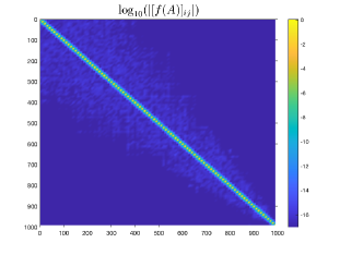
(a)

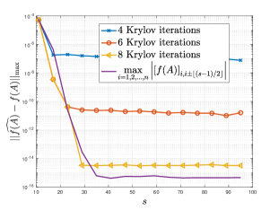
(b)

Figure 1: $f$ is the exponential function $e^{x}$ and $\bm{A}\in\mathbb{R}^{1000\times 1000}$ is a symmetric $2$-banded matrix. The left figure shows the exponential decay in the entries of $f(\bm{A})$ and the right figure shows that the error analysis in (14) captures the decay rate until the error is dominated by the error from evaluating matrix-vector products using the Krylov method. The stagnation of the $\max\limits_{i=1,2,...,n}\left|[f(\bm{A})]_{i,i\pm(s-1)/2}\right|$ curve is caused by machine precision.

We now devise an algorithm based on the above analysis to approximate matrices that satisfy the exponential off-diagonal decay. The algorithm is given in Algorithm 2, which we call BaMRAM (Banded Matrix Recovery Algorithm using Matvecs).

Algorithm 2 Banded Matrix Recovery Algorithm using Matvecs (BaMRAM)

1:Matrix-vector product function handle $\texttt{mvp}:\bm{x}\mapsto\bm{B}\bm{x}$;
$s=2s_{0}+1$ the number of matrix-vector products; (rec. $s_{0}=10k$ for functions of $k$-banded matrices)

2:$\widehat{\bm{B}}$, $s_{0}$-banded approximation to $\bm{B}$;

3:Compute matrix-vector products $\bm{B}_{s}=\texttt{mvp}\left(\bm{I}_{n}^{(s)}\right)\in\mathbb{R}^{n\times s}$, where $\bm{I}_{n}^{(s)}$ is as in (9)

4:Set the entries of $\widehat{\bm{B}}$ using $\bm{B}_{s}$ and (12)

3.2.1 Complexity of BaMRAM (Alg. 2)

The complexity of BaMRAM is $s$ matrix-vector products with $\bm{B}$. In the case $\bm{B}=f(\bm{A})$ for a $k$-banded matrix $\bm{A}$, we can evaluate $f(\bm{A})\bm{I}_{n}^{(s)}$ using polynomial or rational Krylov depending on $f$ and and the spectrum of $\bm{A}$. Assuming that the Krylov method converges (to sufficient accuracy) in $\mathcal{O}(1)$ iterations and $s=2ck+1$ for some constant $c$, the complexity of BaMRAM is $\mathcal{O}(snk)=\mathcal{O}(nk^{2})$.

If we only have access to the matrix using its transpose, i.e. $\bm{x}\mapsto\bm{A}^{T}\bm{x}$ (or $\bm{x}\mapsto\bm{B}^{T}\bm{x}$), then we can take $f(\bm{A}^{T})\bm{I}_{n}^{(s)}$ (or $\bm{B}^{T}\bm{I}_{n}^{(s)}$) and use the rows of $f(\bm{A}^{T})\bm{I}_{n}^{(s)}$ (or $\bm{B}^{T}\bm{I}_{n}^{(s)}$) to recover the columns of $f(\bm{A})$ (or $\bm{B}$).

3.2.2 Analysis of BaMRAM(Alg. 2)

Here we give theoretical guarantees for BaMRAM. The analysis for BaMRAM is easier and it gives a stronger bound than SpaMRAM as the precise location of the dominant entries and the behaviour of the decay is known. The proof is motivated by Proposition 3.2 in ¹⁵.

Theorem 3.3 (Algorithm 2).

Let $\bm{B}$ be a matrix satisfying

$$\left|\bm{B}_{ij}\right|<C\lambda^{|i-j|}$$ (11)

where $C>0$ and $0<\lambda<1$ are constants. Then the output of BaMRAM, $\widehat{\bm{B}}$, satisfies

$$\left\lVert\widehat{\bm{B}}-\bm{B}\right\rVert_{2}\leq\frac{4C\lambda}{1-\lambda}\lambda^{s_{0}}$$

where $s=2s_{0}+1$.

Proof 3.4.

Define $\bm{E}=\widehat{\bm{B}}-\bm{B}$. We get

$$\left\lVert\widehat{\bm{B}}-\bm{B}\right\rVert_{2}=\left\lVert\bm{E}\right\rVert_{2}\leq\sqrt{\left\lVert\bm{E}\right\rVert_{1}\left\lVert\bm{E}\right\rVert_{\infty}}$$

using a special case of Hölder’s inequality ¹² §2.3.3. We now bound $\left\lVert\bm{E}\right\rVert_{1}$ and $\left\lVert\bm{E}\right\rVert_{\infty}$ using (11). By the construction of $\widehat{\bm{B}}$, the $i$th row of $\bm{E}$ satisfies

$$\left\lVert E(i,:)\right\rVert_{1} \leq\sum_{\ell=-s_{0}}^{s_{0}}\left|\widehat{B}_{i,i+\ell}-B_{i,i+\ell}\right|+\sum_{\ell=s_{0}+1}^{n-i}|B_{i,i+\ell}|+\sum_{\ell=s_{0}+1}^{i-1}|B_{i,i-\ell}|$$

$$\leq 2\sum_{\ell=s_{0}+1}^{n-i}|B_{i,i+\ell}|+2\sum_{\ell=s_{0}+1}^{i-1}|B_{i,i-\ell}|$$

$$<2C\sum_{\ell=s_{0}+1}^{n-i}\lambda^{\ell}+2C\sum_{\ell=s_{0}+1}^{i-1}\lambda^{\ell}$$

$$<4C\lambda^{s_{0}+1}\sum_{\ell=0}^{\infty}\lambda^{\ell}=\frac{4C\lambda}{1-\lambda}\lambda^{s_{0}}.$$

Similarly, the $j$th column of $\bm{E}$ satisfies

$$\left\lVert E(:,j)\right\rVert_{1}<\frac{4C\lambda}{1-\lambda}\lambda^{s_{0}}.$$

Therefore

$$\left\lVert\bm{E}\right\rVert_{1}=\max_{1\leq j\leq n}\left\lVert E(:,j)\right\rVert_{1}<\frac{4C\lambda}{1-\lambda}\lambda^{s_{0}},\qquad\left\lVert\bm{E}\right\rVert_{\infty}=\max_{1\leq i\leq n}\left\lVert E(i,:)\right\rVert_{1}<\frac{4C\lambda}{1-\lambda}\lambda^{s_{0}}.$$

We conclude that

$$\left\lVert\widehat{\bm{B}}-\bm{B}\right\rVert_{2}\leq\frac{4C\lambda}{1-\lambda}\lambda^{s_{0}}.$$

Remark 3.5.

1. When $\bm{B}=f(\bm{A})$ for a $k$-banded matrix $\bm{A}$, we can use $s=2ck+1$ for some integer constant $c>0$. This value of $s$ is motivated by the fact that if $f$ is analytic then $f(\bm{A})$ can be well approximated by a low degree polynomial $p(\bm{A})$ which has bandwidth deg$(p)k$.

2. In Theorem 3.3, if $\lambda\leq 0.9$ then for $\epsilon$ accuracy it suffices to take

   $$s_{0}\geq\frac{\log{(36C)}-\log{\epsilon}}{\log{(\lambda^{-1})}}.$$

3.2.3 Different decay rates

A similar analysis can be performed if the decay rate is different on each side of the diagonal, for example, if the matrix satisfies (7) and (8). The argument is the same with a different definition for $t_{ij}$, which is

$$t_{ij}=\operatorname*{arg\,min}\limits_{\begin{subarray}{c}1\leq j+st\leq n\\ t\in\mathbb{Z}\end{subarray}}\left|j+st-i-\frac{s-1}{2}\frac{\log(\lambda_{1}^{-1})-\log(\lambda_{2}^{-1})}{\log(\lambda_{1}^{-1})+\log(\lambda_{2}^{-1})}\right|$$ (15)

where $\lambda_{1}$ is the decay rate above the diagonal and $\lambda_{2}$ is that below the diagonal. This expression for $t_{ij}$ accounts for the different decay rates and coincides with our analysis in the previous section when $\lambda_{1}=\lambda_{2}$. The algorithm will be the same as BaMRAM with $t_{ij}$ defined as (15). For $s=\left\lfloor{c/\log(\lambda_{1}^{-1})}\right\rfloor+\left\lfloor{c/\log(\lambda_{2}^{-1})}\right\rfloor+1$ for some constant $c>0$, the algorithm will output $\widehat{\bm{B}}$ with upper bandwidth $\left\lfloor{c/\log(\lambda_{1}^{-1})}\right\rfloor$ and lower bandwidth $\left\lfloor{c/\log(\lambda_{2}^{-1})}\right\rfloor$ and $\widehat{\bm{B}}$ will satisfy

$$\left\lVert\widehat{\bm{B}}-\bm{B}\right\rVert_{2}\lesssim e^{-c}$$

which can easily be shown by following the proof of Theorem 3.3.

3.3 Extensions to Kronecker Sum

Some of the results for banded matrices and matrices with exponential off-diagonal decay can be naturally extended to Kronecker sums, which arises, for example in the finite difference discretization of the two-dimensional Laplace operator ⁴⁹. Let $\bm{A}^{(1)},\bm{A}^{(2)}\in\mathbb{R}^{n\times n}$. The Kronecker sum $\mathcal{A}\in\mathbb{R}^{n^{2}\times n^{2}}$ of $\bm{A}^{(1)}$ and $\bm{A}^{(2)}$ is defined by

$$\mathcal{A}=\bm{A}^{(1)}\oplus\bm{A}^{(2)}=\bm{A}^{(1)}\otimes\bm{I}_{n}+\bm{I}_{n}\otimes\bm{A}^{(2)}$$

where $\otimes$ is the Kronecker product, defined by

$$\bm{A}\otimes\bm{B}=\begin{bmatrix}A_{11}\bm{B}&A_{12}\bm{B}&...&A_{1n}\bm{B}\\ A_{21}\bm{B}&A_{22}\bm{B}&...&A_{2n}\bm{B}\\ \vdots&\vdots&\ddots&\vdots\\ A_{n1}\bm{B}&A_{n2}\bm{B}&...&A_{nn}\bm{B}\end{bmatrix}\in\mathbb{R}^{n^{2}\times n^{2}}$$

and $\bm{I}_{n}$ is the $n\times n$ identity matrix.

Suppose $\bm{A}^{(1)}$ and $\bm{A}^{(2)}$ are both banded matrices. Then $\bm{I}_{n}\otimes\bm{A}^{(2)}\in\mathbb{R}^{n^{2}\times n^{2}}$ is a banded matrix with the same bandwidth as $\bm{A}^{(2)}$ and $\bm{A}^{(1)}\otimes\bm{I}_{n}\in\mathbb{R}^{n^{2}\times n^{2}}$ is permutation equivalent to a banded matrix with the same bandwidth as $\bm{A}^{(1)}$ because $\bm{P}(\bm{A}^{(1)}\otimes\bm{I}_{n})\bm{P}^{T}=\bm{I}_{n}\otimes\bm{A}^{(1)}$ where $\bm{P}$ is the perfect shuffle matrix ⁵⁰. With this observation, we can use the recovery technique used for banded matrices in Section 3.1 to recover $\mathcal{A}$ for banded matrices $\bm{A}^{(1)}$ and $\bm{A}^{(2)}$. Suppose that $\bm{A}^{(1)}$ and $\bm{A}^{(2)}$ have bandwidth $k_{1}$ and $k_{2}$ respectively. Notice that to recover $\mathcal{A}$, we need to recover the off-diagonal entries of $\bm{A}^{(1)}$ and $\bm{A}^{(2)}$ to recover the off-diagonal entries of $\mathcal{A}$ and recover $A_{ii}^{(1)}+A_{jj}^{(2)}$ for all $i,j$ to recover the diagonal entries of $\mathcal{A}$. We use the following $(2+2k_{1}+2k_{2})$ matrix-vector products

$$\left[\bm{P}^{T}\begin{bmatrix}\bm{I}_{n}^{(1+2k_{1})}\\ \bm{0}\end{bmatrix},\begin{bmatrix}\bm{I}_{n}^{(1+2k_{2})}\\ \bm{0}\end{bmatrix}\right]\in\mathbb{R}^{n^{2}\times(2+2k_{1}+2k_{2})}$$

to recover $\mathcal{A}$. Since the top left $n\times n$ block of $\mathcal{A}$ equals $A_{11}^{(1)}\bm{I}_{n}+\bm{A}^{(2)}$, which is $k_{2}-$banded, the first $n$ rows of the matrix-vector product with $\begin{bmatrix}\bm{I}_{n}^{(1+2k_{2})}\\ \bm{0}\end{bmatrix}$ recovers $A_{11}^{(1)}\bm{I}_{n}+\bm{A}^{(2)}$ exactly (Theorem 3.1), which in turn recovers all the off-diagonal entries of $\bm{A}^{(2)}$. Similarly, $\bm{P}^{T}\begin{bmatrix}\bm{I}_{n}^{(1+2k_{1})}\\ \bm{0}\end{bmatrix}$ recovers $\bm{A}^{(1)}+A_{11}^{(2)}\bm{I}_{n}$ exactly using $\bm{P}(\bm{A}^{(1)}\otimes\bm{I}_{n})\bm{P}^{T}=\bm{I}_{n}\otimes\bm{A}^{(1)}$. Therefore we get all the off-diagonal entries of $\mathcal{A}$ from recovering $A_{11}^{(1)}\bm{I}_{n}+\bm{A}^{(2)}$ and $\bm{A}^{(1)}+A_{11}^{(2)}\bm{I}_{n}$. The diagonal entries of $\mathcal{A}$ can be recovered from the diagonal entries of $A_{11}^{(1)}\bm{I}_{n}+\bm{A}^{(2)}$ and $\bm{A}^{(1)}+A_{11}^{(2)}\bm{I}_{n}$ by noting

$$A_{ii}^{(1)}+A_{jj}^{(2)}=(A_{ii}^{(1)}+A_{11}^{(2)})+(A_{11}^{(1)}+A_{jj}^{(2)})-(A_{11}^{(1)}+A_{11}^{(2)})$$

for all $i,j$.

For matrices with rapid off-diagonal decay, we can extend the above idea in certain cases. Focusing on the matrix exponential, we have a special relation ¹¹ §10

$$\exp(\bm{A}^{(1)}\oplus\bm{A}^{(2)})=\exp(\bm{A}^{(1)})\otimes\exp(\bm{A}^{(2)}).$$

When $\bm{A}^{(1)}$ and $\bm{A}^{(2)}$ are both banded matrices we can use the same procedure above by applying matrix-vector products with

$$\left[\bm{P}^{T}\begin{bmatrix}\bm{I}_{n}^{(s_{1})}\\ \bm{0}\end{bmatrix},\begin{bmatrix}\bm{I}_{n}^{(s_{2})}\\ \bm{0}\end{bmatrix}\right]\in\mathbb{R}^{n^{2}\times(s_{1}+s_{2})}.$$

for sufficiently large $s_{1}$ and $s_{2}$ that captures the dominant entries of $\exp(\bm{A}^{(1)})$ and $\exp(\bm{A}^{(2)})$ near the main diagonal respectively. This extension is natural and analogous to the extension from recovering banded matrices to recovering matrices with exponential off-diagonal decay earlier this section.

The strategy for recovering banded matrices and approximating matrices with rapid off-diagonal decay can also be used as laid out above in a similar setting involving Kronecker product or sum. Examples include $f(\bm{I}\otimes\bm{A})=\bm{I}\otimes f(\bm{A})$ and the formulae for the cosine and the sine of the Kronecker sum between two matrices ¹¹ §12.

4 Numerical Illustrations

Here we illustrate BaMRAM and SpaMRAM using numerical experiments. In all experiments, we use $20$ iterations of polynomial Krylov method and $50$ sample points for the contour integration from method 2 of ²⁵ to evaluate the matrix-vector products with $f(\bm{A})$. In all of the plots, the $x$-axis denotes the number of matrix-vector products $s$, i.e. $\bm{x}\mapsto f(\bm{A})\bm{x}$, and the $y$-axis denotes the relative error in the $2$-norm with respect to $f(\bm{A})$ obtained by dense arithmetic in MATLAB, i.e., expm, sqrtm and logm. For SpaMRAM, the sparsity parameter $k$ is chosen to be $8$ times smaller than the number of matrix-vector products, i.e., $s=8k$ and the sensing operator $\bm{Y}$ is Gaussian. The experiments were conducted in MATLAB version 2021a using double precision arithmetic.

4.1 Synthetic Examples

We illustrate synthetic examples for BaMRAM and SpaMRAM using the functions $e^{x},\sqrt{1+x}$ and $\log(1+x)$. We consider a synthetic banded matrix and a synthetic sparse matrix given below.

• Banded case: symmetric $2$-banded matrix $\bm{A}_{B}\in\mathbb{R}^{1024\times 1024}$ with its nonzero entries drawn from i.i.d. $\mathcal{N}(0,1)$. $\bm{A}_{B}$ has been rescaled to $\left\lVert\bm{A}_{B}\right\rVert_{2}=0.5$.

• General sparse case: symmetric sparse matrix $\bm{A}_{S}\in\mathbb{R}^{1024\times 1024}$ created using the MATLAB command sprandsym with density $1/1024$. $\bm{A}_{S}$ has been rescaled to $\left\lVert\bm{A}_{S}\right\rVert_{2}=0.5$.

Symmetry was enforced to ensure that the eigenvalues are real, and $\bm{A}_{B}$ and $\bm{A}_{S}$ have been rescaled to ensure that their eigenvalues are sufficiently away from $-1$, which is where $\sqrt{1+x}$ and $\log(1+x)$ have singularities. This was done to ensure that the matrix-vector products $f(\bm{A})\bm{b}$ can be computed with high accuracy with 20 Krylov steps.

Figure 2 shows the accuracy of the two algorithms. For the banded case in Figure 2a, we see that the error decays exponentially until the error is dominated by either the machine precision or the error from computing the matrix-vector products. This exponential decay rate is consistent with Theorem 3.3. For the general sparse case in Figure 2b, the error decays quickly with the number of nonzero entries recovered in each row. The sparsity pattern influences the decay rate of SpaMRAM, making the behaviour of the decay rate more unexpected. This has been shown partially in Theorem 2.1 where the bound depends on the sparsity pattern or more specifically the cardinality of the union of the combined support locations of $\bm{I}_{n},\bm{A},...,\bm{A}^{d}$ in each row for $d$ large enough.

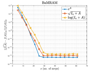
(a)

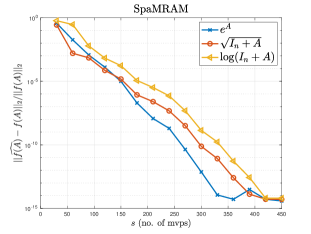
(b)

Figure 2: The accuracy of BaMRAM and SpaMRAM using two $1024\times 1024$ synthetic symmetric matrices: a random $2$-banded matrix (left) and a random sparse matrix with nonzero density $2/1024$ (right).

4.2 Toy Examples

In this section, we manufacture a matrix $\bm{A}$ such that $f(\bm{A})$ has a sparse structure and use our algorithms to approximate $f(\bm{A})$ using matrix-vector products with $\bm{A}$ only. We explore two functions, namely $\sqrt{\bm{A}}$ and $\log{(\bm{A})}$. For the square root function, we set $\sqrt{\bm{A}}$ equal to a sparse positive definite matrix and use our algorithms to recover $\sqrt{\bm{A}}$ via matrix-vector products with $\bm{A}=\left(\sqrt{\bm{A}}\right)^{2}$ (which here is not very sparse). We follow a similar procedure for the matrix logarithm using the formula $\mbox{exp}(\log(\bm{A}))=\bm{A}$. The aim of this experiment is to show that if $f(\bm{A})$ is sparse then we can efficiently recover $f(\bm{A})$ to high accuracy using our algorithms. We choose a sparse positive definite matrix and a banded positive definite matrix from the SuiteSparse Matrix Collection ⁵¹.

• $\mathtt{gr\_30\_30}$: $900\times 900$ $31$-banded symmetric positive definite matrix with $7744$ nonzero entries.

• $\mathtt{Trefethen\_700}$: $700\times 700$ sparse symmetric positive definite matrix with $12654$ nonzero entries and at most $19$ nonzero entries per row and column.

In Figure 3, we see that both matrices are recovered to high accuracy using our algorithms. In Figure 3a, we observe that the matrix $\mathtt{gr\_30\_30}$ is recovered to high accuracy using about $66$ matrix-vector products, which is consistent with the fact that $\mathtt{gr\_30\_30}$ is $31$-banded, and hence has at most $63$ nonzero entries per row and column. In Figure 3b, we see that the matrix $\mathtt{Trefethen\_700}$ has been recovered to high accuracy using about $180$ matrix-vector products. This is fairly consistent with the fact that with $s=180$ matrix-vector products, we recover about $22$ nonzero entries in each row and $\mathtt{Trefethen\_700}$ has at most $19$ nonzero entries per row.

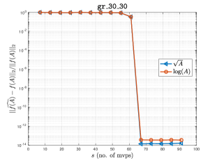
(a)

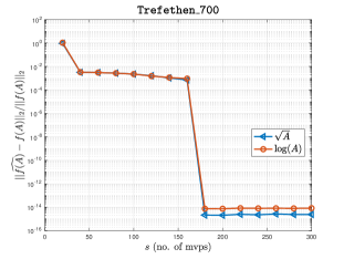
(b)

Figure 3: The accuracy of BaMRAM and SpaMRAM for functions of matrices when $f(\bm{A})$ itself is banded or sparse.

4.3 Sparse dataset examples

We now illustrate BaMRAM and SpaMRAM using the SuiteSparse Matrix Collection ⁵¹, using the four matrices below. The first three matrices are sparse and the last matrix is banded.

• $\mathtt{west1505}$: $1505\times 1505$ sparse matrix with $5414$ nonzero entries and at most $12$ nonzero entries per row and at most $27$ nonzero entries per column.

• $\mathtt{CSphd}$: $1882\times 1882$ sparse matrix with $1740$ nonzero entries and at most $45$ nonzero entries per row and at most $3$ nonzero entries per column.

• $\mathtt{tols2000}$: $2000\times 2000$ sparse matrix with $5184$ nonzero entries and at most $90$ nonzero entries per row and at most $22$ nonzero entries per column.

• $\mathtt{mhd3200b}$: $3200\times 3200$ $18$-banded symmetric positive definite matrix with $18316$ nonzero entries.

For the sparse matrices $\mathtt{west1505}$, $\mathtt{CSphd}$ and $\mathtt{tols2000}$, we use SpaMRAM to recover their matrix exponential. For the banded matrix $\mathtt{mhd3200b}$, we use BaMRAM to recover its matrix exponential, matrix square root and matrix logarithm. The results are illustrated in Figure 4.

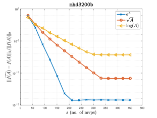
(a)

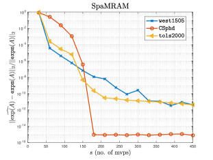
(b)

Figure 4: The accuracy of BaMRAM (left) and SpaMRAM (right) using sparse matrices from ⁵¹.

In Figure 4, we observe that our algorithms are able to approximate $f(\bm{A})$ with good accuracy. In Figure 4a, we notice that the error decreases exponentially until the error stagnates at some point. The stagnation is due to the error incurred in the computation of matrix-vector products $f(\bm{A})\bm{b}$, and can be improved by taking more than 20 Krylov steps. For banded matrices, we consistently obtain exponential convergence rate whose convergence rate is dictated by the smoothness of $f$. In Figure 4b, we note that the error decreases at a rapid speed until it stagnates due to machine precision for $\mathtt{CSphd}$ or slows down due to the sparsity pattern in the case of $\mathtt{west1505}$ and $\mathtt{tols2000}$. As observed in prior experiments, the behaviour is more irregular when the matrix has a more general sparsity pattern.

The approximation to $f(\bm{A})$ in the above experiments can be highly accurate when the bandwidth of the matrix is small or the matrix has a sparsity pattern that makes $f(\bm{A})$ approximately sparse, in the sense that only few entries in each row/column are large in magnitude. Our algorithms are particularly useful when $\bm{A}$ can only be accessed through matrix-vector products and we require an approximation to the entire matrix function. An example is in network analysis where we are given an adjacency matrix $\bm{A}$ and the off-diagonal entries of $e^{\bm{A}}$ describe the communicability between two vertices and the diagonal entries of $e^{\bm{A}}$ describe the subgraph centrality of a vertex ^{52, 53, 5}. The sparse matrix $\mathtt{CSphd}$ in the above experiment is an adjacency matrix for some underlying graph, and with about $180$ matrix-vector products we can approximate its matrix exponential to $10^{-15}$ accuracy. This means that our algorithm can approximate the communicability between any two vertices and the subgraph centrality of any vertex of $\mathtt{CSphd}$ with $10^{-15}$ accuracy.

5 Discussion and extensions

In this paper, we presented two algorithms for approximating functions of sparse matrices and matrices with similar structures using matrix-vector products only. We exploited the decay bound from ¹⁵ to recover the entries of $f(\bm{A})$ that are large in magnitude. The task of approximating functions of matrices is not the only application for SpaMRAM and BaMRAM. These two algorithms can be used more generally in applications where we are able to perform matrix-vector products with the matrix in question and the matrix we want to approximate have the decay bound similar to (5) or (11). An example is the decay bound for spectral projectors ⁵⁴, computed, for example by a discretized contour integral. Therefore the algorithms can be extended naturally to other similar applications.

In many applications, we also want to approximate quantities related to $f(\bm{A})$ such as the trace of $f(\bm{A})$ and the Schatten $p$-norm of $f(\bm{A})$, which for the trace of functions of sparse symmetric matrices has been studied in ⁵⁵. Since SpaMRAM and BaMRAM provide an approximation to $f(\bm{A})$, we can use $\widehat{f(\bm{A})}$ to estimate the quantity of interest. For example, the trace of a matrix function is an important quantity appearing in network analysis through the Estrada index ⁵ and statistical learning through the log-determinant estimation ⁸, among others. Therefore the algorithms can also be used to estimate quantities related to matrix functions.

SpaMRAM uses compressed sensing to recover the matrix function row by row. This algorithm is simple, however we may have access to extra information such as the sparsity pattern of the matrix. This information can potentially be used to speed up the algorithm and increase the accuracy of the algorithm. There are techniques in compressed sensing such as variance density sampling ⁴⁵, which improves signal reconstruction using prior information. The improvement of SpaMRAM and the use of SpaMRAM and BaMRAM in different applications are left for future work.

*Acknowledgements The authors are grateful to Jared Tanner for his helpful discussions and for pointing out useful literature in compressed sensing.

*Funding TP was supported by the Heilbronn Institute for Mathematical Research.

References

- 1 Druskin V, Güttel S, Knizhnerman L. Near-Optimal Perfectly Matched Layers for Indefinite Helmholtz Problems. SIAM Rev. 2016;58(1):90–116.
- 2 Garrappa R, Popolizio M. On the use of matrix functions for fractional partial differential equations. Math Comput Simul. 2011;81(5):1045–1056.
- 3 Grimm V, Hochbruck M. Rational approximation to trigonometric operators. BIT. 2008 jun;48(2):215–229.
- 4 Benzi M, Boito P. Matrix functions in network analysis. GAMM-Mitt. 2020;43(3):e202000012.
- 5 Estrada E, Higham DJ. Network Properties Revealed through Matrix Functions. SIAM Rev. 2010;52(4):696–714.
- 6 Goedecker S. Linear scaling electronic structure methods. Rev Mod Phys. 1999 Jul;71:1085–1123.
- 7 Mohr S, Dawson W, Wagner M, Caliste D, Nakajima T, Genovese L. Efficient Computation of Sparse Matrix Functions for Large-Scale Electronic Structure Calculations: The CheSS Library. J Chem Theory Comput. 2017;13(10):4684–4698.
- 8 Cortinovis A, Kressner D. On randomized trace estimates for indefinite matrices with an application to determinants. Found Comput Math. 2021;22(3):875–903.
- 9 Wenger J, Pleiss G, Hennig P, Cunningham JP, Gardner JR. Preconditioning for Scalable Gaussian Process Hyperparameter Optimization. In: International Conference on Machine Learning (ICML); 2022. .
- 10 Newman MEJ. Finding community structure in networks using the eigenvectors of matrices. Phys Rev E. 2006 Sep;74:036104.
- 11 Higham NJ. Functions of Matrices. SIAM; 2008.
- 12 Golub GH, Van Loan CF. Matrix Computations. 4th ed. Johns Hopkins University Press; 2013.
- 13 Güttel S. Rational Krylov approximation of matrix functions: Numerical methods and optimal pole selection. GAMM-Mitt. 2013;36(1):8–31.
- 14 Güttel S, Kressner D, Lund K. Limited-memory polynomial methods for large-scale matrix functions. GAMM-Mitt. 2020;43(3):e202000019.
- 15 Benzi M, Razouk N. Decay bounds and O(n) algorithms for approximating functions of sparse matrices. ETNA. 2007;28:16–39. Available from: http://eudml.org/doc/130625.
- 16 Candès EJ, Romberg J, Tao T. Robust uncertainty principles: Exact signal reconstruction from highly incomplete frequency information. IEEE Trans Inf Theory. 2006;52(2):489–509.
- 17 Candès EJ, Tao T. Near-Optimal Signal Recovery From Random Projections: Universal Encoding Strategies? IEEE Trans Inf Theory. 2006;52(12):5406–5425.
- 18 Donoho DL. Compressed sensing. IEEE Trans Inf Theory. 2006;52(4):1289–1306.
- 19 Demko S, Moss WF, Smith PW. Decay rates for inverses of band matrices. Math Comp. 1984;43(168):491–499.
- 20 Benzi M, Golub GH. Bounds for the Entries of Matrix Functions with Applications to Preconditioning. BIT. 1999 sep;39(3):417–438.
- 21 Frommer A, Schimmel C, Schweitzer M. Analysis of Probing Techniques for Sparse Approximation and Trace Estimation of Decaying Matrix Functions. SIAM J Matrix Anal Appl. 2021;42(3):1290–1318.
- 22 Coleman TF, Moré JJ. Estimation of Sparse Jacobian Matrices and Graph Coloring Blems. SIAM J Numer Anal. 1983;20(1):187–209.
- 23 CURTIS AR, POWELL MJD, REID JK. On the Estimation of Sparse Jacobian Matrices. IMA J Appl Math. 1974 02;13(1):117–119. Available from: https://doi.org/10.1093/imamat/13.1.117.
- 24 Saad Y. Analysis of Some Krylov Subspace Approximations to the Matrix Exponential Operator. SIAM J Numer Anal. 1992;29(1):209–228.
- 25 Hale N, Higham NJ, Trefethen LN. Computing , , and Related Matrix Functions by Contour Integrals. SIAM J Numer Anal. 2008;46(5):2505–2523.
- 26 Frommer A, Lund K, Szyld DB. Block krylov subspace methods for functions of matrices. ETNA. 2018;27:100–126.
- 27 Cortinovis A, Kressner D, Massei S. Divide-and-Conquer Methods for Functions of Matrices with Banded or Hierarchical Low-Rank Structure. SIAM J Matrix Anal Appl. 2022;43(1):151–177.
- 28 Halikias D, Townsend A. Matrix recovery from matrix-vector products. arXiv preprint arXiv:221209841. 2022;.
- 29 Levitt J, Martinsson PG. Linear-Complexity Black-Box Randomized Compression of Hierarchically Block Separable Matrices. arXiv preprint arXiv:220502990. 2022;.
- 30 Sun X, Woodruff DP, Yang G, Zhang J. Querying a Matrix through Matrix-Vector Products. ACM Trans Algorithms. 2021 oct;17(4).
- 31 Bekas C, Kokiopoulou E, Saad Y. An estimator for the diagonal of a matrix. Applied Numerical Mathematics. 2007;57(11):1214–1229. Numerical Algorithms, Parallelism and Applications (2).
- 32 Herman MA, Strohmer T. High-Resolution Radar via Compressed Sensing. IEEE Trans Signal Process. 2009;57(6):2275–2284.
- 33 Pfander GE, Rauhut H, Tanner J. Identification of Matrices Having a Sparse Representation. IEEE Trans Signal Process. 2008;56(11):5376–5388.
- 34 Dasarathy G, Shah P, Bhaskar BN, Nowak RD. Sketching Sparse Matrices, Covariances, and Graphs via Tensor Products. IEEE Trans Inf Theory. 2015;61(3):1373–1388.
- 35 Candès EJ, Tao T. Decoding by linear programming. IEEE Trans Inf Theory. 2005;51(12):4203–4215.
- 36 Blumensath T, Davies ME, Rilling G. Greedy algorithms for compressed sensing. In: Eldar YC, Kutyniok G, editors. Compressed Sensing: Theory and Applications. Cambridge University Press; 2012. p. 348–393.
- 37 Blanchard JD, Tanner J. Performance comparisons of greedy algorithms in compressed sensing. Numer Linear Algebra Appl. 2015;22(2):254–282.
- 38 Blumensath T, Davies ME. Normalized Iterative Hard Thresholding; Guaranteed Stability and Performance. IEEE J Sel Topics Signal Process. 2010;4(2):298–309.
- 39 Foucart S. Hard Thresholding Pursuit: an Algorithm for Compressive Sensing. SIAM J Numer Anal. 2011;49(6):2543–2563.
- 40 Needell D, Tropp JA. CoSaMP: Iterative signal recovery from incomplete and inaccurate samples. Appl Comput Harmon Anal. 2009;26(3):301–321.
- 41 Foucart S, Rauhut H. A Mathematical Introduction to Compressive Sensing. Applied and Numerical Harmonic Analysis. Springer New York; 2013. Available from: https://books.google.co.uk/books?id=zb28BAAAQBAJ.
- 42 Rokhlin V, Tygert M. A Fast Randomized Algorithm for Overdetermined Linear Least-Squares Regression. Proc Natl Acad Sci USA. 2008;105(36):13212–13217.
- 43 Bayisa FL, Zhou Z, Cronie O, Yu J. Adaptive algorithm for sparse signal recovery. Digital Signal Processing. 2019;87:10–18.
- 44 Indyk P, Price E, Woodruff DP. On the Power of Adaptivity in Sparse Recovery. In: 2011 IEEE 52nd Annual Symposium on Foundations of Computer Science; 2011. p. 285–294.
- 45 Krahmer F, Ward R. Stable and Robust Sampling Strategies for Compressive Imaging. IEEE Trans Image Process. 2014;23(2):612–622.
- 46 Nakos V, Shi X, Woodruff DP, Zhang H. Improved Algorithms for Adaptive Compressed Sensing. In: Chatzigiannakis I, Kaklamanis C, Marx D, Sannella D, editors. 45th International Colloquium on Automata, Languages, and Programming (ICALP 2018). vol. 107 of Leibniz International Proceedings in Informatics (LIPIcs). Dagstuhl, Germany: Schloss Dagstuhl–Leibniz-Zentrum fuer Informatik; 2018. p. 90:1–90:14.
- 47 Benzi M, Simoncini V. Decay Bounds for Functions of Hermitian Matrices with Banded or Kronecker Structure. SIAM J Matrix Anal Appl. 2015;36(3):1263–1282.
- 48 Pozza S, Simoncini V. Inexact arnoldi residual estimates and decay properties for functions of non-Hermitian matrices. BIT. 2019;59(4):969–986.
- 49 LeVeque RJ. Finite Difference Methods for Ordinary and Partial Differential Equations. Steady State and Time Dependent Problems. SIAM; 2007.
- 50 Loan CFV. The ubiquitous Kronecker product. J Comput Appl Math. 2000;123(1):85–100. Numerical Analysis 2000. Vol. III: Linear Algebra.
- 51 Davis TA, Hu Y. The University of Florida Sparse Matrix Collection. ACM Trans Math Softw. 2011 dec;38(1). Available from: https://doi.org/10.1145/2049662.2049663.
- 52 Benzi M, Estrada E, Klymko C. Ranking hubs and authorities using matrix functions. Linear Algebra Appl. 2013;438(5):2447–2474.
- 53 Estrada E, Hatano N. Communicability in complex networks. Phys Rev E. 2008 Mar;77:036111.
- 54 Benzi M, Boito P, Razouk N. Decay Properties of Spectral Projectors with Applications to Electronic Structure. SIAM Rev. 2013;55(1):3–64.
- 55 Frommer A, Rinelli M, Schweitzer M. Analysis of stochastic probing methods for estimating the trace of functions of sparse symmetric matrices. arXiv preprint arXiv:200911392. 2023;.