Efficient Predictive Coding of Intra Prediction Modes

Abstract

The high efficiency video coding (HEVC) standard and the joint exploration model (JEM) codec incorporate 35 and 67 intra prediction modes (IPMs) respectively, which are essential for efficient compression of Intra coded blocks. These IPMs are transmitted to the decoder through a coding scheme. In our paper, we present an innovative approach to construct a dedicated coding scheme for IPM based on contextual information. This approach comprises three key steps: prediction, clustering, and coding, each of which has been enhanced by introducing new elements, namely, labels for prediction, tests for clustering, and codes for coding. In this context, we have proposed a method that utilizes a genetic algorithm to minimize the rate cost, aiming to derive the most efficient coding scheme while leveraging the available labels, tests, and codes. The resulting coding scheme, expressed as a binary tree, achieves the highest coding efficiency for a given level of complexity. In our experimental evaluation under the HEVC standard, we observed significant bitrate gains while maintaining coding efficiency under the JEM codec. These results demonstrate the potential of our approach to improve compression efficiency, particularly under the HEVC standard, while preserving the coding efficiency of the JEM codec.

I Introduction

The latest video coding standard, high efficiency video coding (HEVC) [1], which was finalized in 2013, has achieved a remarkable bitrate reduction of 50% compared to the previous advanced video coding (AVC) standard [2], while maintaining the same subjective quality [3, 4]. In pursuit of even greater coding efficiency, the joint video experts team (JVET), established by motion picture experts group (MPEG) ISO/IEC and international telecommunication union (ITU), has explored new coding tools to develop the versatile video coding (VVC) standard. These proposed coding tools [5, 6] have been incorporated into the joint exploration model (JEM) software, resulting in coding gains of up to 35% [7, 8, 9] when compared to HEVC reference software model (HM) [10]. However, it’s important to note that this coding gain comes at the expense of significantly increased coding complexity, estimated to be 10 times that of HEVC.

This paper focuses on the signaling of intra prediction mode (IPM) in both HEVC and JEM bitstreams. These hybrid video coding schemes employ Intra and Inter predictions to eliminate spatial and temporal correlations in the video sequence, respectively. In recent video coding standards, Intra prediction is performed at the block level and is applied to both Intra and Inter coded slices. The number of IPMs has increased from 14 modes in AVC [11] to 35 and 67 in HEVC and JEM, respectively. These modes cover a wider range of directions towards the reference pixels to enhance the accuracy and efficiency of Intra prediction (See Fig. 1).

However, increasing the number of IPMs results in higher coding complexity and an increased number of bits required to encode the selected IPM at the block level. Several algorithms have been proposed [12, 13, 14] to reduce Intra prediction complexity by testing a restricted set of IPMs with only a slight coding loss. Other complexity reduction techniques focus on predicting block partitioning [15, 16], meaning that Intra prediction modes are tested by the encoder only for certain block configurations. Additionally, signaling more modes would require a higher average number of bits for transmission. To maintain the rate-distortion performance, these modes must be efficiently encoded in the bitstream. In HEVC and JEM, IPMs are efficiently encoded by leveraging contextual information, including the IPMs of neighboring blocks that are already available at the decoder side. Based on this contextual information, these solutions construct a list of most probable modess (MPMs) that are encoded with shorter codes, while the remaining modes are encoded with longer codes. These bits are further compressed using entropy encoding to reduce statistical redundancies.

In this context, authors in [17] have proposed a new ordering of the labels used to construct the MPMs list in the JEM software, based on an offline training process. They defined a total of 4019 possible orderings according to available contextual information, block shape, and depth. This approach resulted in a coding gain of 0.12% at the expense of increased memory usage. However, the training and testing processes were performed on the same video dataset defined in the JEM common test conditions (CTC). Further, authors in [18] introduced two MPM lists (short-term and long-term lists) for more efficient coding of IPMs in the VVC standard. The long-term list captures high correlations with non-adjacent coding units (CUs) within the coding tree unit (CTU), primarily identified in screen content videos. The merge of local and global lists relies on a conditional random field to uniformly model the priority of intra modes. The long-term list is populated using a frequency table of IPMs, which is initialized with predefined tables signaled at the sequence parameter set (SPS) and then updated with selected modes in the CTU. This approach achieved coding gains of 3.75% for screen content videos and 0.1% for natural scene video sequences. Nevertheless, it’s worth noting that the coding schemes for IPMs used in HEVC and JEM are derived empirically based on experimental results. To the best of our knowledge, there is no explicit solution in the literature that derives an optimal signaling scheme for encoding IPMs in video coding standards.

The main contributions of this paper can be summarized as follows:

• We model the construction of efficient signaling schemes for discrete predictive coding based on contextual information.

• We utilize this model to create efficient signaling schemes for IPMs in both reference software implantation of HEVC and JEM.

• Our approach results in a rate-distortion improvement for reference software implantation of HEVC under similar complexity conditions at both the encoder and decoder.

The remainder of this paper is organized as follows. Section II provides background information on Intra prediction and outlines the motivations behind this work. In Section III, we present our proposed model for optimizing code selection using contextual information. Section IV applies the proposed model to HEVC and JEM to construct efficient IPM signaling schemes. The performance of these schemes is assessed in terms of rate-distortion and complexity in Section V. Section VI extends the proposed approach to adaptive dynamic lists for more efficient IPM coding in the JEM reference software. Finally, Section VII concludes the paper.

II Background and motivations

II-A Intra prediction in HEVC and JEM

The HEVC frame is first partitioned into square blocks called CTU of fixed size $N\times N$, with $N\in\{16,\,32,\,64\}$ [19]. Each CTU is partitioned in Quad-Tree to CUs which are then split into prediction units (PUs). The PU represents the base unit for both Intra and Inter predictions. In the case of Intra prediction, the PUs are square of sizes $N\times N$ and $2N\times 2N$ with the associated CU of size $2N\times 2N$, $N\in\{4,8,16\}$. HEVC defines 35 IPMs including 1 planar mode, 1 DC mode and 33 directional modes to predict the PU pixels from the neighbour decoded pixels [20]. The IPMs are signalled in the bitstream to the decoder at the CU level and then all PUs associated to this CU share the same IPM [21].

In the JEM codec, the Quad-Tree partitioning used in HEVC is replaced by the quad-tree plus binary-tree (QTBT) [6] partitioning. The QTBT partitioning first performs a Quad-Tree partitioning of the CTU into CUs which are further partitioned into blocks by Binary-Tree. This later enables horizontal and vertical symmetrical partitioning, which results in more flexible patterns for splitting the blocks leading to better coding efficiency [15]. The blocks corresponding to the splitting of the Binary-Tree are the basis units to perform both Inter and Intra predictions. The Intra prediction in the JEM is performed on blocks of different shapes and sizes. There are in total 67 IPMs including the planar, DC and 65 directional modes.

II-B IPM coding

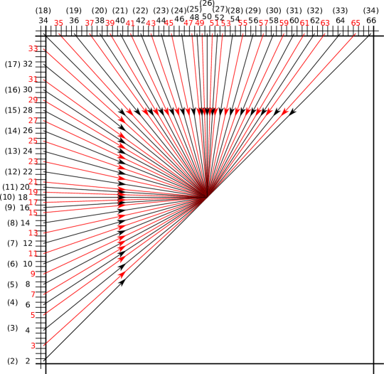
(a) Intra Prediction modes

(b) Neighbour blocks

Figure 1: (a) Angles of the 65 directional IPMs as defined in JEM. The angles in black represent the 33 directional modes available in HEVC, with their numbering from HEVC in parenthesis, and in red the new modes added in the JEM. (b) Positions of blocks coded with IPM $L$, $U$, $BL$, $UR$, $UL$

HEVC uses predictive coding to encode the 35 possible IPMs. The IPMs of left block ($L$) and upper block ($U$) with other numerical modes including 0 (planar), 1 (DC) and 26 (vertical) are used to predict the IPM of the current block and construct its MPMs list of three modes. The first MPM (MPM 0) is encoded with a code of two bits length, the second and third MPMs are signalled by codes of three bits while the remaining 32 IPMs are encoded with codes of 6 bits. Table I gives the codes of the IPM s as defined in the HEVC standard. The first bit of each code, illustrated in red color in Table I, is encoded with the context-adaptive binary arithmetic coding (CABAC) context [22]. The IPM coding scheme in HEVC is noted in the rest of this paper as $2+3+3+(6\times 32)$. This notation gives the number of bits of the three MPMs followed by the number of bits used to code the remaining modes times the number of no MPMs.

The JEM also uses the contextual information to predict the current IPM and construct the MPMs list. The construction of this MPMs list is based on four contexts. As illustrated in Fig. 1b these contexts are the IPM used by the blocks left ($L$), upper ($U$), below left ($BL$), upper right ($UR$) and upper left ($UL$). The JEM defines four specific lists to efficiently encode the IPMs called: MPMs list of 6 modes, Preferred list of 16 modes, other part 1 list of 19 modes and other part 2 list that includes 26 modes. The construction of the MPMs list is filled by including, in this order, modes $L$, $U$, Planar, DC, $BL$, $UR$, $UL$, derived modes ($-1$, $+1$ of the already selected MPMs) and numerical IPMs including $50$ (vertical), $18$ (horizontal), $34$ (diagonal) and $2$ (diagonal). The directions of the 65 angular modes in JEM are shown in Fig. 1a. These modes are included in the MPMs list until this list is filled with 6 different modes. The Preferred list contains modes of indexes from $0$ to $60$ modulo $4$ (i.e. indexes $\in\{0,\,4,\,8,...,\,56,\,60\}$) and not selected as MPMs. The modes of indexes from $0$ to $18$ not present in the MPMs and Preferred lists are used to fill the other part 1 list. Finally, the modes of indexes from $19$ to $45$ and not present in the three previous lists are used to fill the other part 2 list. The 6 MPMs are encoded by 2, 3, 4, 5, 6, and 6 bits, respectively. The 16 IPMs in the Preferred list are coded on 6 bits. The IPMs of the other part 1 and other part 2 lists are coded on 7 and 8 bits, respectively. The coding of IPMs in the JEM is summarized in Table II. The first bits of each mode illustrated in red color in Table II are coded with CABAC contexts while other bits are bypassed. This coding scheme is noted by $2+3+4+5+6+6+(6\times 16)+(7\times 19)+(8\times 26)$ giving the number of bits of the six MPMs followed by the number of bits used to code each of the three other defined lists multiple the number of IPMs within the list.

In all intra (AI) coding configuration, the part of the bitstream related to IPMs represents in average $9\%$ and $5.2\%$ of the whole HEVC and JEM bitstreams, respectively. Therefore, a slight increase in the IPM coding efficiency would result in a significant enhancement in terms of global rate distortion (RD) performance.

TABLE I: used codewords for IPMs in HEVC ($2+3+3+(6\times 32)$). The first bit in red color is coded using a CABAC context while others are coded in ”bypass mode”, with no CABAC context.

IPM s	Codewords	Number of bits
MPM 0	10	2
MPM 1	110	3
MPM 2	111	3
	000000
32 remaining IPM s	$\vdots$	6
	011111

II-C Upper bound performance and motivation

In this section, we evaluate the theoretical limit (empirical entropy) of the IPM coding using contextual information in HEVC and JEM. The entropy is compared to the performance of the codes defined in both HEVC and JEM in terms of average number of bits required to encode the IPM. We consider a dataset composed of 59 heterogeneous video sequences for HEVC and 300 video sequences for the JEM. These video sequences are encoded with HM and JEM reference software in AI coding configuration at 4 different quantization parameters (QPs) $\in\{22,\,27,\,32,\,37\}$ [23]. The coding of IPM is carried out with a fixed length code of 6 bits in HM and 7 bits in the JEM. With a fixed length code, we make sure that the signalling scheme has no impact on the IPM selection, as all modes have the same rate cost, and thus the mode is chosen based on only its corresponding distortion. It should be noted that this configuration is used only to compute the entropy and to train our proposed model. The distribution of data used in here to train our model is not related to a specific coding solution enabling better generalisation of the proposed model.

The entropy computation considers the modes of neighbour blocks in the conditional probability formulation $\mathbb{P}(i|U,L)$ where the modes of upper $U$ and left $L$ blocks are known at the decoder. The HEVC and JEM encodings construct a dataset of $15\times 10^{6}$ and $1.2\times 10^{9}$ samples, respectively, where each sample corresponds to the Intra block and its corresponding IPM and contextual information, i.e. the IPMs neighbour blocks.

TABLE II: Used codewords for IPMs in JEM: $2+3+4+5+6+6+(6\times 16)+(7\times 19)+(8\times 26)$. the first bits in red color are coded using CABAC contexts while others are bypassed.

IPM s	Codewords	Number of bits
MPM 0	10	2
MPM 1	110	3
MPM 2	1110	4
MPM 3	1111 0	5
MPM 4	1111 10	6
MPM 5	1111 11	6
	01 0000
Preferred list ($\times 16$)	$\vdots$	6
	01 1111
	00 00000
Other part 1 list ($\times 19$)	$\vdots$	7
	00 10010
	00 100110
Other part 2 list ($\times 26$)	$\vdots$	8
	00 111111

The entropy of coding IPM using the contextual information $L$ and $U$ is computed as follows

$$\begin{split}\mathbb{H}(\lx@glossaries@gls@link{main}{IPM}{\leavevmode IPM},L,U)=&-\sum_{L=-1}^{K-1}\sum_{U=-1}^{K-1}\mathbb{P}(L,U)\\ &\,\sum_{i=0}^{K-1}\mathbb{P}(i|L,U)\,\,\log_{2}\,\mathbb{P}(i|L,U),\end{split}$$ (1)

where $K$ is the number of IPMs and $\mathbb{P}(L,U)$ is the probability of the left IPM being equal to mode $L$ and the upper IPM being equal to mode $U$. $\mathbb{P}(i|L,U)$ is the conditional probability of the selected IPM being equal to $i$ in the case of the left IPM is equal to $L$ and the above IPM is equal to $U$ with $L,U\in\{-1,0,1,\dots,K-1\}$. This conditional probability considers the contextual information from known left and upper Intra modes. The specific case of $X=-1$ refers to the context $X$ is not available. To compute the empirical entropy, we first estimate from the available prediction modes of the considered dataset the probabilities $\mathbb{P}(L,U)$ and $\mathbb{P}(i|L,U)$ with $L,U\in\{-1,0,1,\dots,K-1\}^{2}$ and $i\in\{0,1,\dots,K-1\}$, then apply Equation  (1) to compute the empirical entropy.

Under the HEVC dataset, the $\mathbb{H}(\lx@glossaries@gls@link{main}{IPM}{\leavevmode IPM},L,U)$ is equal to $3.36$ bits while the HEVC coding scheme achieves $3.86$ bits/mode on the same dataset. Concerning the JEM, we compute the entropy with using $L$, $U$, $BL$, $UR$ and $UL$ modes as available contextual information

$$\begin{split}\mathbb{H}&(\lx@glossaries@gls@link{main}{IPM}{\leavevmode IPM},L,U,\dots,UL)=\\ &-\sum_{L=-1}^{K-1}\sum_{U=-1}^{K-1}\dots\sum_{UL=-1}^{K-1}\mathbb{P}(L,U,\dots,UL)\\ &\sum_{i=0}^{K-1}\mathbb{P}(i|L,U,\dots,UL)\log_{2}\,\mathbb{P}(i|L,U,\dots,UL).\end{split}$$ (2)

The entropy $\mathbb{H}(\lx@glossaries@gls@link{main}{IPM}{\leavevmode IPM},L,U,UL)$ is equal to $3.32$ bits while the JEM code enables $3.44$ bits/mode. Table III gives the entropy of the IPM in the HEVC and JEM without and with using $L$, $U$ $BL$, $UR$ and $UL$ as contextual information for prediction. By definition, the empirical entropy only provides a lower bound estimation for the amount of information contained in the signal [24]. This means that the value estimated by (2) is always lower than the actual information contained in the signal. Adding more data samples reduces the error made by the estimation. One possible correction is the Miller-Madow (MM) bias correction [25] which corrects the entropy by adding $\frac{\tilde{m}-1}{2B}$, where $\tilde{m}$ is an estimation of the number of bins with non-zero probability (for IPM it is the number of possible values {$L$, $U$, $UR$, $UL$, $BL$, IPM } which is equal to $67^{6}$) and $B$ is the number of considered samples (in our case the number of samples in the JEM dataset is $1.2\times 10^{9}$). The values of Miller-Madow (MM) correction are equal to 0 bits/IPM from 0 to 2 contexts, $0.008$ bits/IPM for 3 contexts, $0.275$ bits/IPM for 4 contexts and $1.18$ bits/IPM for 5 contexts. Therefore, the empirical entropy computed with more than four contexts is not reliable since the error is high compared to the computed entropy.

The difference between the computed entropy and the performance of HEVC IPMs coding, estimated to $0.5$ bits/mode in Table III, clearly shows that there is a room for improvement of the IPM coding scheme. This motivates the design of more efficient codes that outperform the existing codes under similar coding/decoding complexities. However, the JEM performance is close to the estimated entropy and thus the objective of the proposed approach is to derive a simple coding scheme with similar coding efficiency and complexity than the JEM. Finally, the developed approach would be generic in the way that it can be applied to any other discrete predictive coding using contextual information such as other video syntax elements including motion vectors.

TABLE III: Entropy and Miller-Madow (MM) correction in bits using $L$, $U$, $UR$, $BL$, $UR$ and $UL$ contextual information in HM and JEM datasets.

Codec	HEVC		JEM
	Entropy	MM	Entropy	MM
$\mathbb{H}(\lx@glossaries@gls@link{main}{IPM}{\leavevmode IPM})$	$4.73$	$0$	$4.66$	$0$
$\mathbb{H}(\lx@glossaries@gls@link{main}{IPM}{\leavevmode IPM},L)$	$3.91$	$0$	$3.79$	$0$
$\mathbb{H}(\lx@glossaries@gls@link{main}{IPM}{\leavevmode IPM},L,U)$	$3.36$	$0$	$3.37$	$0$
$\mathbb{H}(\lx@glossaries@gls@link{main}{IPM}{\leavevmode IPM},L,U,UL)$	–	–	$3.32$	$0.008$
$\mathbb{H}(\lx@glossaries@gls@link{main}{IPM}{\leavevmode IPM},L,U,UR,UL)$	–	–	$3.19$	$0.275$
$\mathbb{H}(\lx@glossaries@gls@link{main}{IPM}{\leavevmode IPM},L,U,BL,UR,UL)$	–	–	$2.99$	$1.18$
Anchors	${\color[rgb]{1,0,0}3.86}$		${\color[rgb]{1,0,0}3.44}$

III Predictive coding model of IPM

In this section the predictive coding using contextual information is modelled in three main steps: prediction, clustering and coding. For each step, examples with the IPM coding schemes used in HEVC and JEM are provided.

III-A Prediction

Prediction enables to reduce the entropy of the information to encode with using already known side information. In video coding continuous prediction is used to predict the pixels based on previously decoded pixels within the same frame for Intra prediction or previously decoded frames for Inter prediction. The prediction of IPM belongs to the discrete (non-continuous) prediction. The prediction of IPM is carried out with contextual information including the IPM of already coded neighbour blocks as well as some specific numerical modes with high probability to be selected. These IPMs used as predictors are referred in this paper as labels.

HEVC defines 7 labels for the prediction of the IPM which are based on two contextual information: IPM of the left block ($L$) and IPM of the upper block ($U$). Four labels in HEVC are based on these two contextual information: $L$, $U$, two angular neighbours of mode $L$ ($L+1$ and $L-1$) as well as three numerical IPMs: 0 (planar), 1 (DC) and 26 (vertical direction). The JEM defines a set 15 labels from 5 contextual information including IPMs of the left block ($L$, $L\pm 1$), the upper block ($U$, $U\pm 1$), below left block ($BL$, $BL\pm 1$), upper right block ($UR$, $UR\pm 1$), upper left block ($UL$, $UL\pm 1$) and six numerical IPMs: Planar, DC, $50$ (vertical), $18$ (horizontal), $34$ (diagonal) and $2$ (the other diagonal). In total, the JEM defines a larger set of 21 labels instead of only seven in HEVC.

III-B Clustering

Clustering is the step that enables to distinguish data following its probability distribution. Better performance will usually be achieved if a prediction is flexible or robust in the sense of being able to fit the local statistical behaviour of the signal [26]. In other words, a smart prediction should adapt to the source at hand. This enables better conditioning and reduces the global entropy of the system [27]. To perform clustering, a set of tests is defined to build a binary-tree where the leaves vertices represent the different clusters of labels and the nodes vertices correspond to tests.

In HEVC, four different tests are defined to separate the labels into five clusters. Fig. 2 illustrates the binary-tree used in HEVC to build these five clusters of labels represented by the leaves vertices and the used tests given by the labelled vertices. The tests leverage the two contextual labels: $L$ and $U$ while the clusters of the three labels represent all possible MPMs lists. The used tests focus mainly on finding whether the two modes $L$ and $U$ are equal and whether they are angular (i.e. $L>1$) or not.

The JEM defines more tests to build the binary-tree with leaves vertices representing the different clusters of six labels. We do not give here the binary-tree of the JEM since it consists of 460 leaves and 196 different labellings composed of a list of 21 available labels. Moreover, the predictive coding of IPM in the JEM was not designed as a decision tree. In fact, the JEM uses a dynamic list to construct the MPMs list based on an ordered list of labels: the labels are added to the MPMs list while checking, for each additional label, whether the corresponding IPM is already in the MPMs list or not.

Figure 2: HEVC binary-tree used to create the MPM list. The code used is $2+3+3+(6\times 32)$.

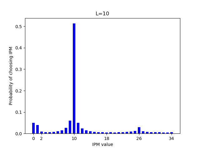
(a) IPM probabilities $L=10$

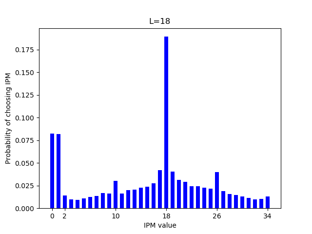
(b) IPM probabilities $L=18$

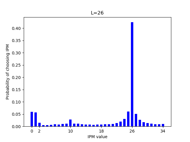
(c) IPM probabilities $L=26$

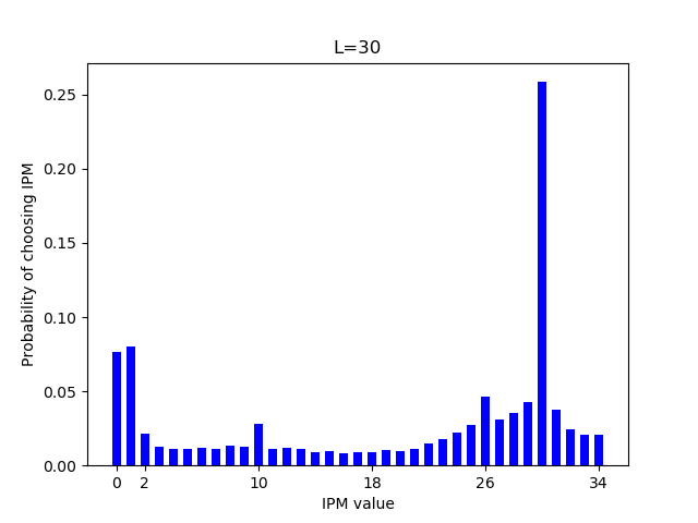
(d) IPM probabilities $L=30$

Figure 3: Probability distribution $\mathbb{P}(i|L)$ of choosing an IPM $i\in\{0,1,\dots,35\}$ when the IMP of the left neighbour block $L$ is: (a) $L=10$, (b) $L=18$, (c) $L=26$, (d) $L=30$. The data is from the HM training set encoded in All Intra configuration at 4 QPs

.

III-C Coding

The coding step defines the codes used to signal the selected IPM at the encoder to the decoder. An efficient coding would allocate a short length code to the most probable modes and longer length code for the rest of modes. After the construction of the binary tree by the clustering step, the coding step allocates a specific code for the IPMs included in the different lists. One code for all the MPM lists (leaves vertices or clusters) can be used, or multiple-code can be used, one specific code for each MPMs list (one specific code by leave vertex or cluster).

In HEVC, variable length (VL) code is used to encode all IPMs within the MPMs list (one VL code for all leaves vertices) and one fixed length (FL) code is used to encode the remaining IPM not present in the selected MPMs list. The codes used in HEVC are depicted in Table I. As for HEVC, JEM uses one VL code to all possible modes in MPMs list. Moreover, the JEM defines three other FL codes to encode the IPMs in the three other lists: Preferred, Other part 1 and Other part 2 as depicted in Table II.

In this section we have modelled the predictive coding of IPM in three steps: prediction, clustering and coding. We have also defined the labels, tests and codes used to encode the IPMs in both HEVC and JEM. In the next sections, we improve these three steps to enhance the coding performance of both HEVC and JEM with defining additional labels, tests, codes and thus new binary trees to reach higher coding performance.

IV Efficient coding schemes of IPMs in HEVC and JEM

IV-A Improved predictive coding

In this section the three predictive coding steps for IPM coding in both HEVC and JEM are improved. The improvements proposed for HEVC and JEM are investigated separately since the same level of complexity with the anchor codes defined in HEVC and JEM is targeted, respectively.

IV-A1 HEVC

To improve the prediction coding of IPM in HEVC, we first introduce additional labels to extend the list of labels to better leverage contextual information. The new list of labels includes the 7 labels defined in HEVC and 23 new labels resulting in a new list of 30 contextual labels and 5 numerical modes. Fig. 3d gives the conditional probability distribution of the IPM $\mathbb{P}(i|L)$ when the mode of the left neighbour block is equal to 10, 18 26 and 30. We can notice from this figure that in addition to the DC and PL modes, the probabilities of modes around the $L$ mode are also high compared to the rest of modes. This motivates including up to six modes around both left ($L$) and ($U$) modes as labels. The new labels are selected from the labels leading to highest conditional probabilities $\mathbb{P}(i|L)$, $\mathbb{P}(i|U)$ with $i\in\{L,U,L\pm 1,U\pm 1,L\pm 2,U\pm 2,L\pm 3,U\pm 3,\dots\}$ as well as the most used numerical modes. The selected labels are $labels\in\{L,\,U,\,L\pm 1,\,0,\,1,\,26,\,U\pm 1,\,L\pm 2,\,L\pm 3,\,U\pm 2,\,U\pm 3,\,\min(L,\,U),\max(L,\,U),\,\min(L,\,U)\pm 1,\,\max(L,\,U)\pm 1,\,\min(L,\,U)\pm 2,\,\max(L,\,U)\pm 2,\,\min(L,\,U)\pm 3,\,\max(L,\,U)\pm 3,|1-min(L,U)|,\,(L+U)/2,\,18,\,2\}$.

To leverage these new labels, new tests are also added to the four HEVC tests set: $tests\in\{L==U,\,|L-U|<2,\,|L-U|==2,\,\min(L,U)>1,\,\min(L,U)<1,\,\max(L,U)<2,\,L+U<2,\,|L-10|<3,\,|L-26|<3,\,|L-18|<3,\,|U-10|<3,\,|U-26|<3,\,|U-18|<3,\,L<2\}$. These new tests are then derived to improve the clustering by finding more similarities. For example, the test $|L-U|<2$ is added as an extension to the test $L==U$. This new test, when $L$ and $U$ are angular, allows detecting whether the two modes are really close to each other. Other new tests check the proximity of the vertical, horizontal and diagonal directions (resp. 26, 10 and 18). Tests using the labels $\min(L,U)$ and $\max(L,U)$ are also proposed. The tests $\min(L,U)>1$ and $\max(L,U)<2$ are added to determine whether the modes are both angular or non-angular ($PL$ or $DC$).

The last step consists in defining the used codes at each cluster. These codes will also determine the number of MPMs within the cluster. A list of VL codes is created, including all codes for clusters of 3 to 7 MPMs. These codes represent all possible VL codes with 3 to 7 bits and FL codes for the rest of symbols. This results in 4 different codes using 3 MPMs, 8 using 5 MPMs and 43 using 7 MPMs for a total of 55 different codes. We consider in this work two configurations: the first one, similar to HEVC and JEM, that uses only one code for all clusters while the second configuration that defines different codes for the clusters.

This new set of codes enables a new theoretical limit on the best achievable cost. The value of $3.45$ bits/IPM is the entropy of the data. To achieve such performance the system would need to use an entropy encoder for all bits of the coding scheme. Moreover, it would require the use of all possible coding schemes for 35 symbols (for which there are 108,861,148 possibilities [28]), and not only the 55 codes described above. This list of codes motivates the computation of another theoretical limit which considers only the 55 selected codes.

Equation (1) is modified to model this description and compute what we define as the empirical code-based entropy. The term $-\log_{2}\mathbb{P}\left(i|L,U\right)$ in (1) is replaced with the used code-length to encode the IPM $i$ knowing the IPMs of left and upper neighbour blocks $L$ and $U$, respectively.

$$\begin{split}&\mathbb{H}_{CB}(\lx@glossaries@gls@link{main}{IPM}{\leavevmode IPM},L,U)=\\ &\sum_{L=-1}^{K-1}\sum_{U=-1}^{K-1}\,\sum_{i=0}^{K-1}\mathbb{P}(i|L,U)\,\,CodeL(i|L,U).\end{split}$$ (3)

This results in a system with $K\times K$ clusters (with $K=35$ in HEVC and $67$ for JEM), each cluster uses the most efficient code among the 55 codes. In HEVC, the code-based entropy achieves a performance of $3.52$ bits/IPM. The signalling scheme giving this value can be created. However, it cannot be implemented because of the high number of clusters. In practice, implementing such a system would require having a table of 1225 entries, each one contains the code and labels to use, which is not acceptable for real time applications. This value asserts that the created systems can reduce the average cost of IPM signalling in HEVC when the chosen tests and labels allow to reach this limit for a small number of clusters.

It should be noted that all these labels, tests and codes will be considered to construct the binary tree of our signalling scheme while only few selected labels, tests and codes will be used within the final binary tree. The selection is performed by a genetic algorithm described in the next section.

TABLE IV: Code-based entropy (CBE) and Miller-Madow (MM) correction in bits using $L$, $U$, $UR$, $BL$, $UR$ and $UL$ contextual information on HM and JEM datasets.

Codec	HEVC		JEM
	CBE	MM	CBE	MM
$\mathbb{H}_{CB}(\lx@glossaries@gls@link{main}{IPM}{\leavevmode IPM})$	$4.84$	$0$	$4.70$	$0$
$\mathbb{H}_{CB}(\lx@glossaries@gls@link{main}{IPM}{\leavevmode IPM},L)$	-	-	$3.85$	$0$
$\mathbb{H}_{CB}(\lx@glossaries@gls@link{main}{IPM}{\leavevmode IPM},L,U)$	$3.52$	$0$	$3.43$	$0$
$\mathbb{H}_{CB}(\lx@glossaries@gls@link{main}{IPM}{\leavevmode IPM},L,U,UL)$	-	-	$3.39$	$0.008$
$\mathbb{H}_{CB}(\lx@glossaries@gls@link{main}{IPM}{\leavevmode IPM},L,U,UR,UL)$	-	-	$3.29$	$0.275$
$\mathbb{H}_{CB}(\lx@glossaries@gls@link{main}{IPM}{\leavevmode IPM},L,U,BL,UR,UL)$	-	-	$3.10$	$1.18$
Anchors	${\color[rgb]{1,0,0}3.86}$		${\color[rgb]{1,0,0}3.44}$

IV-A2 JEM

Three new lists of labels, tests and codes are defined for the JEM. The list of labels contains 57 labels based on three modes from contextual information $L$, $U$ and $UL$, derived modes from these three modes and numerical modes. We also define 41 tests to leverage the considered 57 labels and build the binary tree. We define codes to encode the clusters of 3 to 9 IPMs. We use 4, 8, 47 and 89 codes for lists of 3, 5, 7 and 9 MPMs, respectively, resulting in 148 codes. The new entropy with this set of codes can be computed from (2) by replacing the term $-\log_{2}{\left(\mathbb{P}\left(i|L,U,\dots,UL\right)\right)}$ by the code-length of the IPM $i$ ($i\in\{0,\,1,\,...,\,66\}$) knowing the modes of left, upper and upper left neighbour blocks are equal to $L$, $U$ and $UL$, respectively.

The code-based entropy $\mathbb{H}_{CB}$ computed for the JEM dataset with $L,U$ and $UL$ as contextual information is equals to $3.40$ bits/IPM. We can notice that this code-based entropy is close to the JEM performance of $3.44$ bits/IPM. Therefore, there is less gain to reach with the JEM ($<0.1$ bits/IPM) than for HEVC $0.34$ bits/IPM. The objective for the JEM is then to achieve the entropy performance of $3.4$ bits/IPM by a simple coding scheme obtained with the proposed method. Finally, Table IV summarises the code-based entropy of the HEVC and JEM with using the considered codes and contextual information $L$, $U$, $UR$, $BL$, $UR$ and $UL$.

IV-B Optimal search and limitations

The objective of this work is to derive the most efficient signalling scheme of IPMs. Therefore, we need to assert the efficiency of the proposed approach. This latter can be extended to search for the best signaling scheme of other video syntax elements.

We separate the problem into three parts: 1) how to choose the best performing labels and tests, 2) how to perform the most efficient prediction on a leaf from the available set of labels and 3) how to choose the best clustering from the available set of tests.

IV-B1 Choosing labels and tests

The labels and tests are used for prediction and clustering, respectively. In fact, some labels cannot be used without the proper tests. For instance, labels $L$ and $U$ cannot be used together in the same cluster if no test such as $L=U$ distinguishes equality between these two modes from other cases.

When choosing tests and labels, it is hard to assert that the solution is optimal. There are as many possible tests as there are functions that use the available contexts to separate the space into two clusters. We have also several labels defined by functions combining the available contexts. The possible functions cannot all be evaluated to assert that the best performing tests and labels have been selected. Moreover, we restrict the study to simple tests and simple labels as we do not want to use tests that combine several tests in the form ”$L\neq U~{}and~{}L<18~{}and~{}U>26$”. However, we can try to simulate what the best performing labels with the best clustering would look like. We can then select our tests and labels based on this system, to ensure that the best performing tests and labels are included in the considered sets.

The upper bound theoretical limit is computed by the code-based entropy described in Section IV-A. It provides the best signalling scheme that can be implemented as it computes the cost of the signalling scheme that uses all possible individual clusters (i.e. the maximum number of clusters). We propose the evaluation of a new limit, similar to the code-based entropy, but for a given (and small) number of clusters. This way a limited number of codes is used and the cases with similar statistics are merged into the same cluster.

No assumptions are made on the available tests and labels. While the resulting system can be implemented, and consists of a real signalling scheme, the limitation on its implementation is the same as with the code-based entropy: implementation would require a complete table of all possible values of the contexts containing the corresponding cluster and the used codes. This shows the performance that can be achieved with perfect tests and labels but with a limited number of clusters. Therefore, the perfect tests and labels configuration would rely on a look-up table to derive the corresponding cluster whatever the value of the contextual information (ie. L and U modes in the case of HEVC). This configuration relying on look-up table is not suitable in our system for complexity and memory overheads, while it is used to assess the efficiency of the selected tests and labels.

A genetic algorithm [29] is used to create this signalling scheme. Genetic algorithms are adaptive heuristic search algorithm based on the evolutionary ideas of natural selection and genetics [30]. They also enable intelligent and efficient exploitation of random search.

In this experiment, the $K\times K$ possible context values ($U$ and $L$) are initialized with a random cluster value. From this parent clustering, some children are generated with small changes on the parent: some context values are affected by other clusters. The best result in terms of rate cost computed by (3) of all current parents and children is always kept as a parent for the next iteration, as well as some other randomly selected children. There is no proof that the clustering generated from this genetic search is optimal. The goal is to be able to observe the data, to see which statistics are similar and thus should use a similar code. When using only two contexts, we can observe the results on a plan which is useful to select the appropriate tests.

IV-B2 Labelling selection

This task searches for the best compatible $M$ labels used at each leaf, with $M$ being the number of MPMs. The labels are compatible on a given leaf if whatever the values of the contexts in this leaf, a couple of labels will always correspond to two different IPMs. Otherwise, the signalling scheme will not be valid resulting in two codewords encoding the same IPM. As there are as many codewords as IPMs, one IPM cannot be encoded and correctly transmitted to the decoder.

An exhaustive search would result in testing all possible combinations of labels for a given number of MPMs to see which ones provide valid combinations. Performing this search on all leaves would be extremely costly in terms of computational complexity: to choose 7 MPMs out of 35 labels there are ${35}\choose{7}$ $=6,724,520$ combinations, while this search needs to be done for every available code. We propose to use an alternative approach enabling to provide the most efficient labelling while decreasing the exhaustive search complexity. The proposed algorithm consists in performing a greedy search carried out on all the labels. In a greedy search, the goal is to maximize the gain at each step. For the label search it means always starting from the available labelling with the lowest cost. Fig. 4 gives an example the label search algorithm.

The algorithm starts with the best possible list of labels by selecting the most probable labels and puts them in the MPMs list. The list is then checked for validity on the leaf by asserting that whatever the context values, all labels are compatible (i.e. all labels are always two by two different). In the case of incompatibility, two new lists are created: each with one of the two conflicting labels removed and replaced by the following label with the highest probability in the list. The two newly created lists are added to a queue, and the next list to test is the one with the smallest cost from the queue. The cost in bits/IPM is computed by (3).

Label	$L$	$U$	0	1	26	$L+1$	$L-1$
Probability	35.9%	34.8%	11.2%	10.6%	6.5%	4.3%	4.1%
($\times 100\%$)

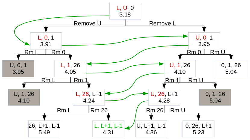
Figure 4: An example of the path followed by the selection algorithm to find the best labelling. In this case the available labels are the ones used by HEVC. The code used to evaluate the labels is $2+3+3+(6\times 32)$. Conflicts are highlighted in red, and the cost in bits/IPM is shown for each tested labelling. The path followed by the algorithm is shown in green. The gray blocks are not evaluated as they are already explored.

It can be shown that all labellings are tested in increasing cost order, and that the best labelling is always added to the queue, and thus tested by the algorithm. Therefore, the first labelling for which all labels are compatible is selected as the most efficient one.

IV-B3 Clustering selection

Two different algorithms are studied for the clustering: one for HEVC and one for the JEM. We target for HEVC a maximum of 8 different clusters and binary-tree with depth 4. Therefore, we can afford performing an exhaustive search over all possible combinations of tests.

However, the JEM coding scheme requires higher number of clusters and deeper binary-tree, so this exhaustive search becomes complex, especially when searching binary-trees with a depth higher than 4. Therefore, the tests will be combined using a genetic search algorithm. This genetic algorithm starts from a binary-tree with random selection of tests and, at each iteration, randomly changes some tests. The best performing configuration is kept for the next iteration as well as some of the created children.

IV-C Optimal clustering search validation

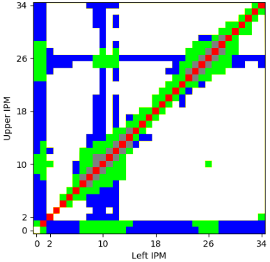
(a) Perfect labels and tests (3.53 bits/IPM)

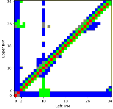
(b) Labels from the new list of labels and perfect tests (3.60 bits/IPM)

Figure 5: Clustering results according to the left and upper IPM. The five clusters are illustrated in different colors.

Fig. 5 shows the results of the genetic clustering for 5 clusters (similar to HEVC) using (a) perfect labels and tests, (b) labels from the proposed list of labels and perfect tests. These two configurations enable coding efficiencies on the training set of 3.53 and 3.60 bits/IPM, respectively. The 5 clusters are illustrated with different colour codes with respect to the left $L$ and upper $U$ IPMs. This clustering asserts whether the selected labels and tests are sufficient or we need to add new ones. The red cluster is used when $L$ and $U$ are equal and the white cluster represents the case where $L$ and $U$ are not equal and different from 0 and 1. The rest of the clustering is harder to interpret but there seem to be differences when L or U are not both angular; when L and U are close but not equal; when L is close to 10 (horizontal mode); when U is close to 26 (vertical mode). Those last three cases are not represented by any leaf in the HEVC binary-tree. As all those tests are available in our list of tests, we can assume that our tests are diverse enough.

We can notice that clustering in Fig. 5b is close to the one using perfect labels illustrated in Fig. 5a. This asserts that the proposed labels is close to the perfect labels. However, this clustering cannot be reproduced by a simple tree since the perfect test is supposed. This means that the performance of this signalling can only be obtained with a high number of leaves. However, if the tests and labels are efficient enough to reproduce this clustering, this would mean having a tree that uses 3.60 bits/IPM, which would be a significant improvement over the HEVC signalling scheme, which uses 3.86 bits/IPM.

TABLE V: Test video sequences

Class	Name	Resolution	Frame	Number
			rate (fps)	of frames
A1	CampfireParty	3840$\times$2160	30	300
	Drums		100	300
JEM	Tango		60	294
	ToddlerFountain		60	300
A2	CatRobot	3840$\times$2160	60	300
	DaylightRoad		30	300
JEM	RollerCoaster		60	300
	TrafficFlow		60	300
A	NebutaFestival	2560$\times$1600	30	150
	PeopleOnStreet		30	150
HEVC	SteamLocomotiveTrain		30	150
	Traffic		30	150
B	BasketballDrive1	1920$\times$1080	24	240
	BQTerrace		24	240
	Cactus		50	500
	Kimono1		50	500
	ParkScene		60	600
C	BasketballDrill	832 $\times$ 480	24	240
	BQMall		24	240
	PartyScene		24	240
	RaceHorses		24	240
D	BasketballPass	416 $\times$ 240	24	240
	BlowingBubbles		24	240
	BQSquare		24	240
	RaceHorses		24	240
E	FourPeople	1280 $\times$ 720	24	240
	Johnny		24	240
	KristenAndSara		24	240
F	BasketballDrillText	832 $\times$ 480	24	240
	ChinaSpeed	1024 $\times$ 468	24	240
HEVC	SlideEditing	1280 $\times$ 720	24	240
	SlideShow	1280 $\times$ 720	24	240

The results of this genetic clustering are similar on the JEM but harder to illustrate as more than two contexts are used. The efficiency of the proposed solution for the JEM signalling scheme also needs to be assessed by comparing the trees of small depths created with the genetic algorithm to the best trees using the same number of leaves, found with an exhaustive search. As those results were perfectly identical for every number of compared leaves, up to trees with 8 leaves and depth 4, we confirm that a genetic algorithm is appropriate for this problem.

Therefore, the resulting trees, presented in the next section, are validated close to the best available for the considered sets of tests and labels.

V Results and discussions

V-A Experimental setup

We consider video sequences for evaluation from HEVC and JEM CTCs [23, 31]. The two video sets, described in Table V, are identical except for class A which is different and class F is optional in the JEM CTC. The test set video sequences are then encoded with both the HM and JEM encoders at four QP $\in\{22,\,27,\,32,\,37\}$ in AI coding configuration. The native IPM signalling schemes in the HM and JEM represent the anchors while the modified with the our signalling schemes represent the proposed schemes. The performance of these latter is assessed in terms of average number of bits per IPM, Bjøntegaard delta bit rate (BD-BR) [32, 33] and codec complexity with respect to the anchors.

V-B Results and Analysis

V-B1 Performance versus HEVC

Figure 6: Average bits/IPM for the two evaluated system setups for different number of clusters. The black lines represent the two limits described in the previous Section.

The first experiment consists in measuring the efficiency of the created signalling schemes on the testing datasets in bits/IPM. This is performed outside the codec, simply based on the previously discussed dataset. Fig. 6 shows the performance in bits/IPM of different signalling schemes created from the proposed list of tests, labels and codes with different numbers of clusters from 3 to 8. The performance is provided for the proposed scheme in two configurations using one code and multiple codes for the different clusters. The proposed solution is compared to HEVC, code-based entropy and entropy. We can notice that even with using less clusters, the proposed scheme enables better coding efficiency compared to HEVC.

We can also notice that multiple codes configuration performs better than using only one code for all the clusters. Moreover, the multiple codes configuration converges faster toward the optimal solution (ie. the code-based entropy). The performance of the most efficient created system with 8 leaves is close by 0.05 bits/IPM from the best achievable system. This confirms the efficiency of the considered tests and labels.

As HEVC uses a signalling scheme with 5 clusters, the signalling scheme that we propose for integration in the HM and comparison in terms of rate distortion is the one using 5 clusters. This scheme is presented as a binary decision tree in Fig. 7. This figure gives the selected tests to perform clustering and the used codes by the five clusters.

Figure 7: Selected system for HEVC shown as a decision tree. For each cluster the used code is shown below it. For clarity $min(U,L)$ and $max(U,L)$ are simply written $min$ and $max$. The colours refer to the clustering shown in Fig. 8.

The clustering representation of this scheme is illustrated in Fig. 8b with respect to left and upper modes $L$ and $U$. We can notice from this figure that the new labels and tests enable better clustering than HEVC clustering illustrated in Fig. 8a. Moreover, the clustering of the proposed scheme is close from the clustering derived with perfect tests illustrated in Fig. 5b, which asserts the efficiency of the proposed list of tests. Moreover, some tests are used enabling the use of some specific labels: for example the test $max<2$ is used to leverage the numerical labels 10, 26, 2 and 34 on the second leaf as they could not be used on the first leaf along with $max(L,U)$.

This signalling scheme uses 4 different codes on the 5 different clusters where 3 of those 4 codes use 7 MPMs. The only cluster using a 5-MPMs code is the one where both IPMs are angular and are not close to each other ($min(L,U)>1$ is true and $|L-U|<2$ is false, corresponding to the yellow cluster in Fig. 8). Another main difference with HEVC is the use in the MPMs list of the two non-angular modes, either through the use of the labels $min(L,U)$ and $|min(L,U)-1|$ on the leaves 0 and 1 (as, on these leaves, per the first test we know that the minimum between $L$ and $U$ is either 0 or 1, $min(L,U)$ and $|min(L,U)-1|$ refer to 0 and 1 or 1 and 0) or explicitly as 0 and 1 on the other leaves.

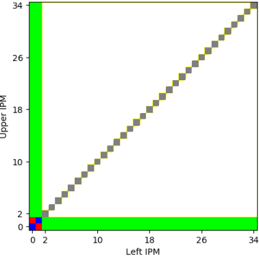
(a) HEVC clustering

(b) Proposed clustering

Figure 8: The clustering of the 5-leaf signalling scheme. Each colour represents a cluster.

This system has been selected to be tested in the HM codec under the CTC in AI coding configuration. Table VI gives the BD-BR of the proposed codes with respect to the two anchors HM and JEM, respectively. For HEVC, the proposed coding scheme enables -0.18% bitrate gain on average on all test sequences. Moreover, all sequences benefit from this new signalling scheme. Such gains are extremely interesting as they do not add significant complexity at both encoder and decoder. The encoding and decoding run times are presented in Table VII. The results published in [34] and [35] emphasis better BD-BR results ($-0.4\%$) with similar systems, it has to be noted that their implementations do not consider the complexity introduced by the increased number of MPM for the RD search in HEVC. The implementation for the system proposed in this work asserts that the number of modes tested in RD remains exactly the same as for the anchor. This coding efficiency can be further improved by considering coding schemes with higher number of clusters up to 8 clusters at the expense of slight increase in the codec complexity.

V-B2 Performance versus JEM

Figure 9: Average bits/IPM for the two evaluated system setups for different number of clusters. The black lines represent the two limits described in the previous Section. The JEM signalling scheme is put here for comparison but actually uses 460 clusters.

Fig. 9 gives the performance of the proposed signalling scheme in average number of bits/IPM for different number of clusters in comparison with the code-based entropy and entropy. The performance of the proposed signaling scheme is close to the code-based entropy with using only 3 contexts ($L$, $U$ and $UL$) where JEM uses 5 contextual information since it also uses $BL$ and $UR$. Moreover, the JEM uses 460 different leaves and 196 different labellings while our signalling scheme relies on only 12 leaves.

An interesting observation that cannot be seen simply by looking at the number of bits/IPM in Fig. 9 is that the trees only use tests and labels relying on $L$ and $U$ up to 7 clusters (and therefore $UL$ context is not used in trees with less than 8 clusters). It means that the tests based on $UL$ provide much less information than those based on $L$ and $U$, and this explains why so many clusters are required by the JEM to efficiently use $BL$ and $UR$.

The scheme with 12-leaf tree is only 0.05 bits/IPM away from the JEM performance, we think appropriate to test it under the CTCs and see if our simplification of the JEM signaling scheme provides good RD performance. As the JEM signalling scheme uses 4 different CABAC contexts, our proposed signalling scheme also relies on only 4 CABAC contexts. On each leaf one CABAC is used on the first bit of the code. The leaves are grouped so that leaves with similar probabilities for this first bit uses the same CABAC context.

The 12-leaf tree enables similar coding efficiency as the JEM under the CTCs in AI coding configuration with +0.03% BD-BR increase on average on the test sequences, as illustrated in Table VI.

The encoding and decoding times are presented in Table VII. The new code used for HEVC slightly increases the codec complexity caused by the 3 used CABAC contexts while only one context is used by HEVC. For the JEM, the complexity remains similar with the anchor at both encoder and decoder since they use the same number of 5 CABAC contexts. This complexity performance proves the method’s efficiency to provide efficient and simple signalling schemes. Moreover, the proposed codes are also simpler than the one used in the JEM as they only use a list of MPMs followed by a unique code-length, while the JEM code uses 3 different code-lengths for its non-predicted modes.

TABLE VI: BD-rate gains in AI coding configuration under CTC

Class	Name	HEVC	JEM
A1	CampfireParty	-	0.07%
	Drums	-	-0.08%
	Tango	-	-0.04%
	ToddlerFountain	-	0.13%
A2	CatRobot	-	-0.02%
	DaylightRoad	-	0.09%
	RollerCoaster	-	-0.05%
	TrafficFlow	-	0.03%
A	NebutaFestival	-0.07%	-
	PeopleOnStreet	-0.27%	-
	SteamLocomotiveTrain	-0.12%	-
	Traffic	-0.15%	-
B	BasketballDrive1	-0.19%	0.07%
	BQTerrace	-0.13%	0.21%
	Cactus	-0.18%	0.01%
	Kimono1	-0.17%	-0.01%
	ParkScene	-0.14%	0.14%
C	BasketballDrill	-0.27%	0.18%
	BQMall	-0.12%	0.02%
	PartyScene	-0.09%	0.10%
	RaceHorses	-0.18%	-0.04%
D	BasketballPass	-0.06%	0.06%
	BlowingBubbles	-0.09%	0.00%
	BQSquare	-0.09%	0.16%
	RaceHorses	-0.18%	0.02%
E	FourPeople	-0.24%	-0.05%
	Johnny	-0.25%	-0.13%
	KristenAndSara	-0.29%	-0.15%
F	BasketballDrillText	-0.20%	-
	ChinaSpeed	-0.27%	-
	SlideEditing	-0.14%	-
	SlideShow	-0.41%	-
-	Average	-0.18%	+0.03%

VI Dynamic lists

We can notice from the previous section that the coding performance of the proposed solution is quite similar to the anchor JEM. Moreover, the BD-BR increase for some sequences like BQTerrace or BasketballDrill is mainly caused to the distribution of IPMs in these sequences, which is not well leveraged by the proposed coding scheme. In this section we propose a combination of dynamic lists and decision tree to build a more efficient coding scheme of the JEM IPMs.

VI-A Labels Used in Dynamic Lists

The JEM uses 21 labels in its dynamic list: the 5 neighbouring IPM s $L$, $U$, $UL$, $UR$ and $BL$, the corresponding directional neighbours of those modes $L\pm 1$, $U\pm 1$, … and 6 numerical labels, 0, 1, 2, 18, 34 and 50. To create a more efficient dynamic list than the one defined in the JEM, it is necessary to include new labels that can enhance the prediction.

Labels are selected in the same way as in the previous section: the existing labels are extended in order to be able to capture more information. The labels presented in our proposed list consist of the JEM modes and more directional neighbours for the present modes ($L\pm 3$, $L\pm 4$, …). All directional modes are also used, giving a final list of 117 labels, including the 67 numerical labels and 50 labels based on contextual information.

To perfectly reproduce the performance of the JEM code, labels that can replicate the preferred list are needed. Those would be labels based on the numerical values of the previously used modes in the MPM list. However, using those labels increases the search for the best order of labels by a factor of 10. Due to this increase in complexity it was chosen not to use such modes in the presented dynamic lists.

VI-B Creating Dynamic Lists

A dynamic list is an ordering of a list of labels. From the list of 117 available labels there are therefore $117!=4\times 10^{192}$ possible dynamic lists. To handle such levels of complexity, a genetic algorithm is used to order the labels. The genetic algorithm works as a guided random search. One candidate solution is an order of labels. Its cost is evaluated by creating the probability histogram of indexes containing 67 values. On this histogram all available codes are tested, and the most efficient one is kept. The mutations for this genetic algorithm consist in operations changing the order of labels, such as swapping two labels, inserting a label in a random position, etc. As there is still no certainty on the optimality of the genetic algorithm, safety checks are performed. This latter performs changes on the final lists obtained to see if its performance can be enhanced. The overall order is kept but the cost is measured for every change of position for individual label in the list.

TABLE VII: encoding and decoding times in AI coding configuration in CTC compared to respective anchors.

	HEVC		JEM
Class	Enc. Time	Dec. Time	Enc. Time	Dec. Time
A1	-	-	100%	99%
A2	-	-	101%	101%
A	103%	106%	-	-
B	104%	103%	100%	100%
C	103%	98%	100%	100%
D	104%	101%	100%	100%
E	104%	99%	101%	100%
F	104%	101%	-	-
Average	104%	102%	100%	100%

VI-C Combining Dynamic Lists and Decision Trees

One of the most advantages presented in our previous section is the use of multiple codes in the designed signalling schemes. Using different codes allows better fit of the probability distributions. Therefore, we propose to combine a decision tree with dynamic lists to enable using different codes and different predictions. On each leaf of the decision tree, one dynamic list can be created with its corresponding code. This way both the prediction and the code better fit the different clusters.

To create those decision trees, the proposed tests are based on the same contextual information as the labels. It appeared that having tests solely based on $L$ and $U$ was sufficient for creating efficient decision trees, as those two labels alone captured most of the information. Moreover, including additional neighbour modes would require more complex decision tree to leverage this contextual information. In our approach, one dynamic list is created for each leaf, and since this is a time consuming process, as explained in the previous section, small decision trees are preferred.

VI-D Experimental results

The designed trees incorporate 4 leaves, each linked to a dynamic list, as illustrated in Fig. 10. Each dynamic list (leaf) employs a distinct code. Additionally, a single CABAC context is employed for the first bit of each code. Consequently, the designed schemes utilize a total of 4 distinct CABAC contexts, which is fewer than the five contexts employed by the JEM. The training process for constructing these dynamic lists is an iterative one, involving multiple training passes. In the initial pass, samples from the JEM native codes are used, while in the subsequent passes, samples encoded by the codes generated in the preceding pass are utilized. Furthermore, it’s important to note that different datasets are employed in the training process for constructing the dynamic lists in each pass.

TABLE VIII: Results in bits/IPM of the different pass for dynamic lists using a decision tree. The reference (Ref) in Pass 1 is the JEM. The reference of each row then corresponds to the New of the previous row. Delta is $\frac{New-Ref}{Ref}$.

	JEM	Ref	New	Delta
Pass 1	3.416	3.416	3.436	0.59%
Pass 2	3.426	3.287	3.251	-1.10%
Pass 3	3.414	3.299	3.283	-0.48%
Pass 4	3.410	3.287	3.282	-0.15%

Table VIII shows the results in bits/IPM of the proposed scheme after each pass. The first pass corresponds to data encoded with the JEM encoder. On this set, the designed tree is not as efficient as the JEM in terms of bits/IPM. Training sequences are encoded using this designed decision tree, to provide a training set for the second pass. A second dynamic tree is designed from this list. It uses the same tests as the previous one with different order of modes for the MPM lists and new codes at each leaf. The dynamic lists built from the second pass enable a reduction of 1.1% in terms of bits/IPM. For the third pass, a gain in bits/IPM is still observed but it is more than halved compared with the previous pass. As the tree designed for a fourth pass shows an even smaller improvement in bits/IPM. At this stage, convergence seems reached, and we decided to not to perform further passes, nor to implement this tree. Fig. 10 shows the tree trained in the third pass as well as the codes (up to the first fixed length code) used at each leaf. This tree achieved 3.283 bits/IPM for the training set resulting from the pass 3, and 3.287 on the training set of the 4th pass.

Table IX presents the results in BD-rate of the successively implemented trees under the CTCs. The first observation is that, even if the tree designed from the first pass performs theoretically worse than the JEM, it achieves a BD-rate gain of 0.04%. This is a small gain, but considering that it uses one less CABAC context than the JEM it is promising. The use of multiple passes is then proved to be efficient, since the gains are increased to 0.09% for the third pass. The small decrease in BD-rate between the second and third pass confirms that convergence has been reached and that no further pass should be able to reduce the coding efficiency.

Figure 10: Number of bits used on each leaf of the decision tree for dynamic lists. On the left is the number of bits, multiplied by the number of symbols when necessary. Bits in bold are coded using a CABAC context. One CABAC context is used by leaf.

TABLE IX: Results in BD-BR of the tree using dynamic labelling on each leaf, against JEM in AI. The tree designed in the first pass uses data from JEM 7 encoding, and then each tree uses data encoded using the previous pass.

Class	Pass 1	Pass 2	Pass 3
A1	-0.02%	-0.06%	-0.07%
A2	0.00%	-0.07%	-0.07%
B	0.7%	0.03%	0.02%
C	-0.05%	-0.06%	-0.15%
D	-0.06%	-0.11%	-0.10%
E	-0.24%	-0.29%	-0.23%
F	0.00%	-0.14%	-0.11%
Average	-0.04%	-0.08%	-0.09%

With a particular list, some optimisations can be made to reduce the number of tests made to create the dynamic list. These optimisations already performed by the JEM. Such optimisations are not considered for the presented lists, which is why no consideration should be taken for the complexity. An example of optimisation is, to stop using the dynamic list as soon as the remaining modes in the list are all coded using the same number of bits. This has no impact on the performance but reduces the number of tests performed and therefore the complexity. The same kind of optimisations can be made on all leaves. After these optimisations, the designed system should have the same complexity as the JEM, as it has been made sure that no extra modes are tested during the RD-search. Compared to recent methods proposed to encode the IPMs [17, 18], our technique enables coding performance in the same range of 0.1% BD-BR gain under the JEM codec without increasing the complexity at both encoder and decoder sides. Under the HM software, the BD-BR gain of 0.18% is even higher with a slight complexity increase of 104% and 102% at encoder and decoder sides, respectively. These results clearly show the ability of the proposed method to derive efficient predictive coding schemes to encode IPMs.

VII Conclusion

In this paper, we have developed a discrete prediction coding model that leverages contextual information in three key steps: prediction, clustering, and coding. To enhance these steps, we have introduced novel labels for prediction, tests for clustering, and codes for coding. We employ a genetic algorithm to select the optimal combinations of labels, tests, and codes that minimize the rate cost. This modeling approach has been applied to derive optimal coding schemes for IPMs in both the HM and JEM reference software. It allows approaching the code-based entropy while increasing the number of clusters. These newly proposed coding schemes have been seamlessly integrated into the HM and JEM codecs. Under the HEVC CTCs, our proposed scheme with 5 clusters has yielded a coding efficiency improvement of -0.18% while maintaining the same complexity level. In the case of the JEM, the new scheme featuring 12 clusters has achieved coding performance comparable to the anchor scheme. Additionally, our research has demonstrated that combining dynamic lists with a simple decision tree results in superior coding performance compared to the JEM under the same complexity constraints.

References

- [1] G. J. Sullivan, J.-R. Ohm, W.-J. Han, and T. Wiegand, “Overview of the High Efficiency Video Coding (HEVC) Standard,” IEEE Transactions on Circuits and Systems for Video Technology, vol. 22, no. 12, pp. 1649–1668, Dec. 2012. [Online]. Available: http://ieeexplore.ieee.org/lpdocs/epic03/wrapper.htm?arnumber=6316136
- [2] T. Wiegand, G. Sullivan, G. Bjontegaard, and A. Luthra, “Overview of the H.264/AVC video coding standard,” IEEE Transactions on Circuits and Systems for Video Technology, vol. 13, no. 7, pp. 560–576, Jul. 2003. [Online]. Available: http://ieeexplore.ieee.org/lpdocs/epic03/wrapper.htm?arnumber=1218189
- [3] J.-R. Ohm, G. J. Sullivan, H. Schwarz, T. K. Tan, and T. Wiegand, “Comparison of the Coding Efficiency of Video Coding Standards - Including High Efficiency Video Coding (HEVC),” IEEE Transactions on Circuits and Systems for Video Technology, vol. 22, no. 12, pp. 1669–1684, Dec. 2012. [Online]. Available: http://ieeexplore.ieee.org/lpdocs/epic03/wrapper.htm?arnumber=6317156
- [4] T. K. Tan, R. Weerakkody, M. Mrak, N. Ramzan, V. Baroncini, J.-R. Ohm, and G. J. Sullivan, “Video Quality Evaluation Methodology and Verification Testing of HEVC Compression Performance,” IEEE Transactions on Circuits and Systems for Video Technology, vol. 26, no. 1, pp. 76–90, Jan. 2016. [Online]. Available: http://ieeexplore.ieee.org/lpdocs/epic03/wrapper.htm?arnumber=7254155
- [5] X. Zhao, J. Chen, M. Karczewicz, A. Said, and V. Seregin, “Joint Separable and Non-Separable Transforms for Next-Generation Video Coding,” IEEE Trans. Image Process., vol. 27, no. 5, pp. 2514–2525, May 2018.
- [6] Z. Wang, S. Wang, J. Zhang, S. Wang, and S. Ma, “Effective quadtree plus binary tree block partition decision for future video coding,” in 2017 Data Compression Conference (DCC), April 2017, pp. 23–32.
- [7] H. Schwarz, C. Rudat, M. Siekmann, B. Bross, D. Marpe, and T. Wiegand, “Coding Efficiency / Complexity Analysis of JEM 1.0 coding tools for the Random Access Configuration,” in Document JVET-B0044 3rd 2nd JVET Meeting: San Diego, CA, USA, February 2016.
- [8] E. Alshina, A. Alshin, K. Choi, and M. Park, “Performance of JEM 1 tools analysis,” in Document JVET-B0044 3rd 2nd JVET Meeting: San Diego, CA, USA, February 2016.
- [9] N. Sidaty, W. Hamidouche, O. Deforges, and P. Philippe, “Compression efficiency of the emerging video coding tools,” in 2017 IEEE International Conference on Image Processing (ICIP), Sep. 2017, pp. 2996–3000.
- [10] HHI, “HM reference software for HEVC.” https://hevc.hhi.fraunhofer.de, 2017.
- [11] A. K. Khan and H. Jamal, “The intra prediction in h.264,” in Novel Algorithms and Techniques In Telecommunications, Automation and Industrial Electronics, T. Sobh, K. Elleithy, A. Mahmood, and M. A. Karim, Eds. Dordrecht: Springer Netherlands, 2008, pp. 11–15.
- [12] H. Zhang and Z. Ma, “Fast Intra Mode Decision for High Efficiency Video Coding (HEVC),” IEEE Transactions on Circuits and Systems for Video Technology, vol. 24, no. 4, pp. 660–668, April 2014.
- [13] A. Mercat, F. Arrestier, W. Hamidouche, M. Pelcat, and D. Menard, “Energy Reduction Opportunities in an HEVC Real-Time Encoder,” in Acoustics, Speech and Signal Processing (ICASSP), 2017 IEEE International Conference on. IEEE, 2017.
- [14] S. Ryu and J. Kang, “Machine Learning-Based Fast Angular Prediction Mode Decision Technique in Video Coding,” IEEE Transactions on Image Processing, vol. 27, no. 11, pp. 5525–5538, Nov 2018.
- [15] Z. Wang, S. Wang, J. Zhang, S. Wang, and S. Ma, “Probabilistic Decision Based Block Partitioning for Future Video Coding,” IEEE Transactions on Image Processing, vol. PP, no. 99, pp. 1–1, 2017.
- [16] Z. Jin, P. An, L. Shen, and C. Yang, “CNN oriented fast QTBT partition algorithm for JVET intra coding,” in 2017 IEEE Visual Communications and Image Processing (VCIP), Dec 2017, pp. 1–4.
- [17] M. Jiang, S. Li, N. Ling, J. Zheng, and P. Zhang, “On Derivation of Most Probable Modes for Intra Prediction in Video Coding,” in 2018 IEEE International Symposium on Circuits and Systems (ISCAS), May 2018, pp. 1–4.
- [18] J. Li, M. Wang, L. Zhang, K. Zhang, H. Liu, S. Wang, S. Ma, and W. Gao, “Unified intra mode coding based on short and long range correlations,” IEEE Transactions on Image Processing, vol. 29, pp. 7245–7260, 2020.
- [19] P. Helle, S. Oudin, B. Bross, D. Marpe, M. O. Bici, K. Ugur, J. Jung, G. Clare, and T. Wiegand, “Block Merging for Quadtree-Based Partitioning in HEVC,” IEEE Transactions on Circuits and Systems for Video Technology, vol. 22, no. 12, pp. 1720–1731, Dec 2012.
- [20] J. Lainema, F. Bossen, W. J. Han, J. Min, and K. Ugur, “Intra Coding of the HEVC Standard,” IEEE Transactions on Circuits and Systems for Video Technology, vol. 22, no. 12, pp. 1792–1801, Dec 2012.
- [21] H. Chen, T. Zhang, M. Sun, A. Saxena, and M. Budagavi, “Improving Intra Prediction in High-Efficiency Video Coding,” IEEE Transactions on Image Processing, vol. 25, no. 8, pp. 3671–3682, Aug 2016.
- [22] V. Sze and M. Budagavi, “High Throughput CABAC Entropy Coding in HEVC,” IEEE Transactions on Circuits and Systems for Video Technology, vol. 22, no. 12, pp. 1778–1791, Dec 2012.
- [23] V. Seregin and Y. He, “Common SHM test conditions and software reference configurations.” CTVC document JCTVC-Q1009, Apr. 2014.
- [24] L. Paninski, “Estimation of Entropy and Mutual Information,” Neural Comput., vol. 15, no. 6, pp. 1191–1253, Jun. 2003. [Online]. Available: http://dx.doi.org/10.1162/089976603321780272
- [25] C. R. Blyth, “Note on Estimating Information,” The Annals of Mathematical Statistics, vol. 30, no. 1, pp. 71–79, 1959.
- [26] A. Gersho and R. M. Gray, Vector Quantization and Signal Compression, ser. The Springer International Series in Engineering and Computer Science. Englewood Cliffs, N.J: Springer, 1992.
- [27] M. J. Weinberger, G. Seroussi, and G. Sapiro, “The LOCO-I lossless image compression algorithm: principles and standardization into JPEG-LS,” IEEE Transactions on Image Processing, vol. 9, no. 8, pp. 1309–1324, Aug 2000.
- [28] N. J. A. Sloane, A Handbook of Integer Sequences, A. Press, Ed. MIT Press [u.a.], 1973, oCLC: 254943406.
- [29] J. McCall, “Genetic algorithms for modelling and optimisation,” Journal of Computational and Applied Mathematics, vol. 184, no. 1, pp. 205 – 222, 2005, special Issue on Mathematics Applied to Immunology.
- [30] B. B. Pal, S. Roy, and M. Kumar, “A Genetic Algorithm to Goal Programming Model for Crop Production with Interval Data Uncertainty,” in Handbook of Research on Natural Computing for Optimization Problems. IGI Global, 2016, pp. 30–65.
- [31] K. Suehring and X. Li, “JVET common test conditions and software reference configurations,” in JVET-B1010, 2016.
- [32] G. Bjøntegaard, “Calcuation of Average PSNR Differences Between RD-curves,” in VCEG-M33 ITU-T Q6/16, Austin, TX, USA, 2-4 April, 2001.
- [33] G. Bjøntegaard, “Improvements of the BD-PSNR model,” ITU-T SG16 Q, vol. 6, p. 35, 2008.
- [34] K. Reuze, P. Philippe, O. Deforges, and W. Hamidouche, “Intra prediction modes signalling in HEVC,” in Picture Coding Symposium (PCS), 2016. IEEE, 2016, pp. 1–5.
- [35] K. Reuzé, P. Philippe, W. Hamidouche, and O. Déforges, “Cluster adapted signalling for intra prediction in HEVC,” in Data Compression Conference (DCC), 2017. IEEE, 2017, pp. 191–200.